
HAL Id: hal-01763422https://hal.archives-ouvertes.fr/hal-01763422
Submitted on 11 Apr 2018
HAL is a multi-disciplinary open accessarchive for the deposit and dissemination of sci-entific research documents, whether they are pub-lished or not. The documents may come fromteaching and research institutions in France orabroad, or from public or private research centers.
L’archive ouverte pluridisciplinaire HAL, estdestinée au dépôt et à la diffusion de documentsscientifiques de niveau recherche, publiés ou non,émanant des établissements d’enseignement et derecherche français ou étrangers, des laboratoirespublics ou privés.
An Online Stochastic Algorithm for a Dynamic NurseScheduling Problem
Antoine Legrain, Jérémy Omer, Samuel Rosat
To cite this version:Antoine Legrain, Jérémy Omer, Samuel Rosat. An Online Stochastic Algorithm for a Dynamic NurseScheduling Problem. European Journal of Operational Research, Elsevier, 2020, 285 (1), pp.196-210.10.1016/j.ejor.2018.09.027. hal-01763422
An Online Stochastic Algorithm for a Dynamic Nurse Scheduling Problem
Antoine Legraina,b, Jeremy Omerc,d, Samuel Rosata,d
aPolytechnique Montreal, 2900, boulevard Edouard-Montpetit, Campus de l’Universite de Montreal, 2500, chemin dePolytechnique, Montreal (QC) H3T 1J4, Canada, www. polymtl. ca
bInteruniversity Research Center on Enterprise Networks, Logistics and Transportation (CIRRELT), Universite deMontreal, Pavillon Andre-Aisenstadt, CP 6128, Succursale Centre-Ville, Montreal (QC) H3C 3J7, Canada, www. cirrelt. ca
cInstitut National de Sciences Appliquees (INSA), 20, avenue des Buttes de Coesmes, 35708 Rennes, France,http: // www. insa-rennes. fr
dGroup for Research in Decision Analysis (GERAD), HEC Montreal, 3000 ch. de la Cote-Sainte-Catherine, Montreal (QC)H3T 2A7, Canada, www. gerad. ca
Abstract
In this paper, we focus on the problem studied in the second international nurse rostering competition: a
personalized nurse scheduling problem under uncertainty. The schedules must be computed week by week
over a planning horizon of up to eight weeks. We present the work that the authors submitted to this
competition and which was awarded the second prize.
At each stage, the dynamic algorithm is fed with the staffing demand and nurses preferences for the
current week and computes an irrevocable schedule for all nurses without knowledge of future inputs. The
challenge is to obtain a feasible and near-optimal schedule at the end of the horizon.
The online stochastic algorithm described in this paper draws inspiration from the primal-dual algorithm
for online optimization and the sample average approximation, and is built upon an existing static nurse
scheduling software. The procedure generates a small set of candidate schedules, rank them according to
their performance over a set of test scenarios, and keeps the best one. Numerical results show that this
algorithm is very robust, since it has been able to produce feasible and near optimal solutions on most of
the proposed instances ranging from 30 to 120 nurses over a horizon of 4 or 8 weeks. Finally, the code of
our implementation is open source and available in a public repository.
Keywords: Stochastic Programming, Nurse Rostering, Dynamic problem, Sample Average Approximation,
Primal-dual Algorithm, Scheduling
1. Introduction
In western countries, hospitals are facing a major shortage of nurses that is mainly due to the overall
aging of the population. In the United Kingdom, nurses went on strike for the first time in history in May
Email addresses: [email protected] (Antoine Legrain), [email protected] (Jeremy Omer),[email protected] (Samuel Rosat)
Preprint submitted to Journal to be determined November 24, 2017

2017. Nagesh [15] says that “It’s a message to all parties that the crisis in nursing recruitment must be put
center stage in this election”. In the United States, “Inadequate staffing is a nationwide problem, and with
the exception of California, not a single state sets a minimum standard for hospital-wide nurse-to-patient
ratios.” [20]. In this context, the attrition rate of nurses is extremely high, and hospitals are now desperate
retain them. Furthermore, nurses tend to often change positions, because of the tough work conditions and
because newly hired nurses are often awarded undesired schedules (mostly due to seniority-based priority in
collective agreements). Consequently, providing high quality schedules for all the nurses is a major challenge
for the hospitals that are also bound to provide expected levels of service.
The nurse scheduling problem (NSP) has been widely studied for more than two decades (refer to [5]
for a literature review). The NSP aims at building a schedule for a set of nurses over a certain period of
time (typically two weeks or one month) while ensuring a certain level of service and respecting collective
agreements. However, in practice, nurses often know their wishes of days-off no more than one week ahead
of time. Managers therefore often update already-computed monthly schedules to maximize the number of
granted wishes. If they were able to compute the schedules on a weekly basis while ensuring the respect
of monthly constraints (e.g., individual monthly workload), the wishes could be taken into account when
building the schedules. It would increase the number of wishes awarded, improve the quality of the schedules
proposed to the nurses, and thus augment the retention rate.
The version of the NSP that we tackle here is that of the second International Nurse Rostering Compe-
tition of 2015 (INRC–II) [6], where it is stated in a dynamic fashion. The problem features a wide variety of
constraints that are close to the ones faced by nursing services in most hospitals. In this paper, we present
the work that we submitted to the competition and which was awarded second prize.
1.1. Literature review
Dynamic problems are solved iteratively without comprehensive knowledge of the future. At each stage,
new information is revealed and one needs to compute a solution based on the solutions of the previous
stages that are irrevocably fixed. The optimal solution of the problem is the same as that of its static (i.e.,
offline) counterpart, where all the information is known beforehand, and the challenge is to approach this
solution although information is revealed dynamically (i.e., online).
Four main techniques have been developed to do this: computing an offline policy (Markov decision
processes [19] are mainly used), following a simple online policy (Online optimization [4] studies these
algorithms), optimizing the current and future decisions (Stochastic optimization [3] handles the remaining
uncertainty), or reoptimizing the system at each stage (Online stochastic optimization [22] provides a general
framework for designing these algorithms).
Markov decision processes decompose the problem into two different sets (states and actions) and two
functions (transition and reward). A static policy is pre-computed for each state and used dynamically at
2

each stage depending on the current state. Such techniques are overwhelmed by the combinatorial explosion
of problems such as the NSP, and approximate dynamic programming [18] provides ways to deal with the
exponential growth of the size of the state space. This technique has been successfully applied to financial
optimization [1], booking [17], and routing [16] problems. In Markof decision processes, most computations
are performed before the stage solution process, therefore this technique relies essentially on the probability
model that infers the future events.
Online algorithms aim at solving problems where decisions are made in real-time, such as online adver-
tisement, revenue management or online routing. As nearly no computation time is available, researchers
have studied these algorithms to ensure a worst case or expected bound on the final solution compared to
the static optimal one. For instance, Buchbinder [4] designs a primal-dual algorithm for a wide range of
problems such as set covering, routing, and resource allocation problems, and provides a competitive-ratio
(i.e., a bound on the worst-case scenario) for each of these applications. Although these techniques can
solve very large instances, they cannot solve rich scheduling problems as they do not provide the tools for
handling complex constraints.
Stochastic optimization [3] tackles various optimization problems from the scheduling of operating
rooms [7] to the optimization of electricity production [9]. This field studies the minimization of a sta-
tistical function (e.g., the expected value), assuming that the probability distribution of the uncertain data
is given. This framework typically handles multi-stage problems with recourse, where first-level decisions
must be taken right away and recourse actions can be executed when uncertain data is revealed. The value
of the recourse function is often approximated with cuts that are dynamically computed from the dual
solutions of some subproblems obtained with Benders’ decomposition. However these Benders-based de-
composition methods converge slowly for combinatorial problems. Namely, the dual solutions do not always
provide the needed information and the solution process therefore may require more computational time
than is available. To overcome this difficulty, one can use the sample average approximation (SAA) [11] to
approximate the uncertainty (using a small set of sample scenarios) during the solution and also to evaluate
the solution (using a larger number of scenarios).
Finally, online stochastic optimization [22] is a framework oriented towards the solution of industrial
problems. The idea is to decompose the solution process in three steps: sampling scenarios of the future,
solving each one of them, and finally computing the decisions of the current stage based on the solution of
each scenario. Such techniques have been successfully applied to solve large scale problems as on-demand
transportation system design [2] or online scheduling of radiotherapy centers [12]. Their main strength is
that any algorithm can be used to solve the scenarios.
3

1.2. Contributions
The INRC–II challenges the candidates to compute a weekly schedule in a very limited computational
time (less than 5 minutes), with a wide variety of rich constraints, and with important correlations between
the stages. Due to the important complexity of this dynamic NSP, none of the tools presented in the
literature review allows to solve this problem. We therefore introduce an online stochastic algorithm that
draws inspiration from the primal-dual algorithms and the SAA. In that method,
• the online stochastic algorithm offers a framework to solve rich combinatorial problems;
• the primal-dual algorithm speeds up the solution by inferring quickly the impact of some decisions;
• the SAA efficiently handles the important correlations between weeks without increasing tremendously
the computational time.
Finally, the algorithm uses a free and open-source software as a subroutine to solve static versions of the
NSP. It is described in details in [13] and summarized in Section 3.
We emphasize that the algorithm described in this article has been developed in a time-constrained
environment, thus forcing the authors to balance their efforts between the different modules of the software.
The resulting code is shared in a public Git repository [14] for reproduction of the results, future comparisons,
improvements and extensions. The remainder of the article is organized as follows. In Section 2, we give
a detailed description of the NSP as well as the dynamic features of the competition. In Section 3, we
state a static formulation and summarize the algorithm that we use to solve it. In Section 4, we present
the dynamic formulation of the NSP, the design of the algorithm, and the articulation of its components.
In Section 5, we give some details on the implementation of the algorithm, study the performance of our
method on the instances of the competition, and compare them to those obtained by the other finalist teams.
Our concluding remarks appear in Section 6.
2. The Nurse Scheduling Problem
The formulation of the NSP that we consider is the one proposed by Ceschia et al. [6] in the INRC–II, and
the description that we recall here is similar to theirs. First, we describe the constraints and the objective
of the scheduling problem Then, we discuss the challenges brought in by the uncertainty over future stages.
The NSP aims at computing the schedule of a group of nurses over a given horizon while respecting a
set of soft and hard constraints. The soft constraints may be violated at the expense of a penalty in the
objective, whereas hard constraints cannot be violated in a feasible solution. The dynamic version of the
problem considers that the planning horizon is divided into one-week-long stages and that the demand for
nurses at each stage is known only after the solution of the previous stage is computed. The solution of each
stage must therefore be computed without knowledge of the future demand.
4

The schedule of a nurse is decomposed into work and rest periods and the complete schedules of all the
nurses must satisfy the set of constraints presented in Table 1. Each nurse can perform different skills (e.g.,
Head Nurse, Nurse) and each day is divided into shifts (e.g., Day, Night). Furthermore, each nurse has
signed a contract with their employers that determines their work status (e.g., Full-time, Part-time) and
work agreements regulate the number of days and weekends worked within a month as well as the minimum
and maximum duration of work and rest periods. For the sake of nurses’ health and personal life and to
ensure a sufficient level of awareness, some successions of shifts are forbidden. For instance, a night shift
cannot be followed by a day shift without being separated by at least one resting day. The employers also
need to ensure a certain quality of service by scheduling a minimum number of nurses with the right skills
for each shift and day. Finally, the length of the schedules (i.e., the planning horizon) can be four or eight
weeks.
Hard constraintsH1 Single assignment per day: A nurse can be assigned at most one shift per day.H2 Under-staffing: The number of nurses performing a skill on a shift must be at least equal to the
minimum demand for this shift.H3 Shift type successions: A nurse cannot work certain successions of shifts on two consecutive
days.H4 Missing required skill: A nurse can only cover the demand of a skill that he/she can perform.Soft constraintsS1 Insufficient staffing for optimal coverage: The number of nurses performing a skill on a shift
must be at least equal to an optimal demand. Each missing nurse is penalized according to a unitweight but extra nurses above the optimal value are not considered in the cost.
S2 Consecutive assignments: For each nurse, the number of consecutive assignments should bewithin a certain range and the number of consecutive assignments to the same shift should also bewithin another certain range. Each extra or missing assignment is penalized by a unit weight.
S3 Consecutive resting days: For each nurse, the number of consecutive resting days should bewithin a certain range. Each extra or missing resting day is penalized by a unit weight.
S4 Preferences: Each assignment of a nurse to an undesired shift is penalized by a unit weight.S5 Complete week-end: A given subset of nurses must work both days of the week-end or none of
them. If one of them works only one of the two days Saturday or Sunday, it is penalized by a unitweight.
S6 Total assignments: For each nurse, the total number of assignments (worked days) scheduled inthe planning horizon must be within a given range. Each extra or missing assignment is penalizedby a unit weight.
S7 Total working week-ends: For each nurse, the number of week-ends with at least one assignmentmust be less than or equal to a given limit. Each worked weekend over that limit is penalized by aunit weight.
Table 1: Constraints handled by the software.
The hard constraints (Table 1, H1–H4) are typical for workforce scheduling problems: each worker
is assigned an assignment or day-off every day, the demand in terms of number of employees is fulfilled,
particular shift successions are forbidden, and a minimum level of qualification of the workers is guaranteed.
5
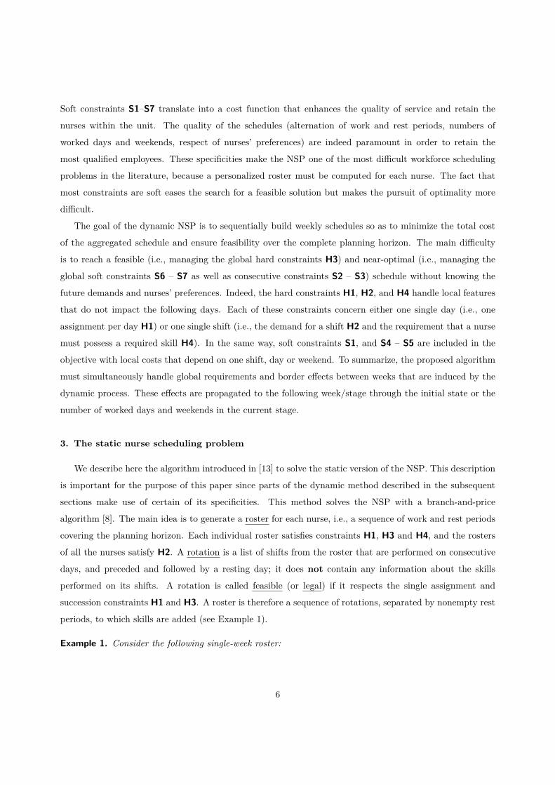
Soft constraints S1–S7 translate into a cost function that enhances the quality of service and retain the
nurses within the unit. The quality of the schedules (alternation of work and rest periods, numbers of
worked days and weekends, respect of nurses’ preferences) are indeed paramount in order to retain the
most qualified employees. These specificities make the NSP one of the most difficult workforce scheduling
problems in the literature, because a personalized roster must be computed for each nurse. The fact that
most constraints are soft eases the search for a feasible solution but makes the pursuit of optimality more
difficult.
The goal of the dynamic NSP is to sequentially build weekly schedules so as to minimize the total cost
of the aggregated schedule and ensure feasibility over the complete planning horizon. The main difficulty
is to reach a feasible (i.e., managing the global hard constraints H3) and near-optimal (i.e., managing the
global soft constraints S6 – S7 as well as consecutive constraints S2 – S3) schedule without knowing the
future demands and nurses’ preferences. Indeed, the hard constraints H1, H2, and H4 handle local features
that do not impact the following days. Each of these constraints concern either one single day (i.e., one
assignment per day H1) or one single shift (i.e., the demand for a shift H2 and the requirement that a nurse
must possess a required skill H4). In the same way, soft constraints S1, and S4 – S5 are included in the
objective with local costs that depend on one shift, day or weekend. To summarize, the proposed algorithm
must simultaneously handle global requirements and border effects between weeks that are induced by the
dynamic process. These effects are propagated to the following week/stage through the initial state or the
number of worked days and weekends in the current stage.
3. The static nurse scheduling problem
We describe here the algorithm introduced in [13] to solve the static version of the NSP. This description
is important for the purpose of this paper since parts of the dynamic method described in the subsequent
sections make use of certain of its specificities. This method solves the NSP with a branch-and-price
algorithm [8]. The main idea is to generate a roster for each nurse, i.e., a sequence of work and rest periods
covering the planning horizon. Each individual roster satisfies constraints H1, H3 and H4, and the rosters
of all the nurses satisfy H2. A rotation is a list of shifts from the roster that are performed on consecutive
days, and preceded and followed by a resting day; it does not contain any information about the skills
performed on its shifts. A rotation is called feasible (or legal) if it respects the single assignment and
succession constraints H1 and H3. A roster is therefore a sequence of rotations, separated by nonempty rest
periods, to which skills are added (see Example 1).
Example 1. Consider the following single-week roster:
6

Day 0 1 2 3 4 5 6
Shift Night Night Rest Rest Early Day RestSkill N N - - HN N -
,
where N stands for Nurse skill and HN for Head Nurse skill. The rotations of that roster, highlighted on the
table above, are (0, Night), (1, Night) and (4, Early), (5, Day).
The MIP described in [13] is based on the enumeration of possible rotations by column generation. As
in most column-generation algorithms, a restricted master problem is solved to find the best fractional
roster using a small set of rotations, and subproblems output rotations that could be added to improve
the current solution or prove optimality. These subproblems are modeled as shortest path problems with
resource constraints whose underlying networks are described in [13]. To obtain an integer solution, this
process is embedded within a branch-and-bound scheme. The remainder of the section focuses on the master
problem. For the sake of clarity, we assume that, for every nurse, the set of all legal rotations is available,
which conceals the role of the subproblem. It is also worth mentioning that the software is based only on
open-source libraries from the COIN-OR project (BCP framework for branch-and-cut-and-price and the
linear solver CLP), and is thus both free and open-source.
We consider a set N of nurses over a planning horizon of M weeks (or K = 7M days). The sets of all
shifts and skills are respectively denoted as Σ and S. The nurse’s type corresponds to the set of skills he
or she can use. For instance, most head nurses can fill Head Nurse demand, but they can also fill Nurse
demand in most cases. All nurses of type t ∈ T (e.g., nurse or head nurse) are gathered within the subset
Nt. For the sake of readability, indices are standardized in the following way: nurses are denoted as i ∈ N ,
weeks as m ∈ 1 . . .M , days as k ∈ 1 . . .K , shifts as s ∈ S and skills as σ ∈ Σ. We use (k, s) to denote
the shift s of day k. All other data is summarized in Table 2.
NursesL−i , L+
i min/max total number of worked days over the planning horizon for nurse iCR−i , CR+
i min/max number of consecutive days-off for nurse iBi max number of worked week-ends over the planning horizon for nurse iDemandDskσ min demand in nurses performing skill σ on shift (k, s)
Oskσ optimal demand in nurses performing skill σ on shift (k, s)Initial stateCD0
i initial number of ongoing consecutive worked days for nurse iCS0
i initial number of ongoing consecutive worked days on the same shift for nurse is0i shift worked on the last day before the planning horizon for nurse iCR0
i initial number of ongoing consecutive resting days for nurse i
Table 2: Summary of the input data.
Remark (Initial state). Obviously, if CR0i > 0, then CD0
i = CS0i = 0, and vice-versa, because the nurse
was either working or resting on the last day before the planning horizon. Moreover, s0i only matters if the
7

nurse was working on that day. The total number of worked days and worked week-ends of a nurse is set at
zero (0) at the beginning of the planning horizon.
The master problem described in Formulation (1) assigns a set of rotations to each nurse while ensuring
at the same time that the rotations are compatible and the demand is filled. The cost function is shaped
by the penalties of the soft constraints as no other cost is taken into account in the problem proposed by
the competition. For any soft constraint SX, its associated unit weight in the objective function is denoted
as cX .
Let Ri be the set of all feasible rotations for nurse i. The rotation j of nurse i has a cost cij (i.e., the
sum of the soft penalties S2, S4 and S5) and is described by the following parameters: askij , akij , and bmij
which are equal to 1 if nurse i works respectively on shift (k, s), on day k, and weekend m, and 0 otherwise.
Finally, f−ij and f+ij represent the first and last worked days of this rotation.
Let xij be a binary decision variable which takes value 1 if rotation j is part of the schedule of nurse i and
zero otherwise. The binary variables rikl and rik measure if constraint S3 is violated: they are respectively
equal to 1 if nurse i has a rest period from day k to l − 1 including at most CR+i consecutive days (cost:
cikl3 ), and if nurse i rests on day k and has already rested for at least CR+i consecutive days before k, and to
zero otherwise. The integer variables w+i and w−i count the number of days worked respectively above L+
i
and below L−i by nurse i. The integer variable vi counts the number of weekends worked above Bi by nurse
i. Finally, the integer variables nskσ , nsktσ , and zskσ respectively measures the number of nurses performing
skill σ, the number of nurses of type t performing skill σ, and the undercoverage of skill σ on shift (k, s).
min∑i∈N
[ ∑j∈Ri
cijxij︸ ︷︷ ︸S2,S4,S5
+CR+
i∑k=1
c3rik +min(K+1,k+CR+
i)∑
l=k+1cikl3 rikl
︸ ︷︷ ︸
S3
+ c6(w+i + w−i )︸ ︷︷ ︸S6
+ c7vi︸︷︷︸S7
]
+ c1
K∑k=1
∑s∈S
∑σ∈Σ
zskσ︸ ︷︷ ︸S1
(1a)
subject to:
[H1,H3] :min(K+1,k+CR+
i)∑
l=k+1rikl −
∑j∈Ri:f+
ij=k−1
xij = 0, ∀i ∈ N ,∀k = 2 . . .K (1b)
[H1,H3] : rik − ri(k−1) +∑
j∈Ri:f−ij=k
xij −k−1∑
l=max(1,k−CR+i
)
rilk = 0, ∀i ∈ N ,∀k = 2 . . .K (1c)
8
[H1,H3] :K∑
l=max(1,K+1−CR+i
)
rilK + riK +∑
j:f+ij
=K
xij = 1, ∀i ∈ N (1d)
[S6] :∑j∈Ri
K∑k=1
akijxij + w−i ≥ L−i , ∀i ∈ N (1e)
[S6] :∑j∈Ri
K∑k=1
akijxij − w+i ≤ L
+i , ∀i ∈ N (1f)
[S7] :∑j∈Ri
M∑m=1
bmijxij − vi ≤ Bi, ∀i ∈ N (1g)
[H2] :∑t∈T σ
nsktσ ≥ Dskσ , ∀s ∈ S, k ∈ 1 . . .K , σ ∈ Σ (1h)
[S1] :∑t∈T σ
nsktσ + zskσ ≥ Oskσ , ∀s ∈ S, k ∈ 1 . . .K , σ ∈ Σ (1i)
[H4] :∑i∈Nt,j
askij xij −∑σ∈Σt
nsktσ = 0, ∀s ∈ S, k ∈ 1 . . .K , σ ∈ Σ (1j)
xij ∈ N, zskσ , nsktσ ∈ R, ∀i ∈ N , j ∈ Ri, s ∈ S, k ∈ 1 . . .K , t ∈ T , σ ∈ Σ (1k)
rikl, rik, w+i , w
−i , vi ≥ 0, ∀i ∈ N , k ∈ 1 . . .K , l = k + 1 . . .min(K + 1, k + CR+
i ) (1l)
where Σt is the set of skills mastered by a nurse of type t (e.g., head nurses have the skills Head Nurse and
Nurse), and T σ is the set of nurse types that masters skill σ (e.g., Head Nurse skill can be only provided by
head nurses).
The objective function (1a) is composed of 5 parts: the cost of the chosen rotations in terms of consecutive
assignments and preferences (S2, S4, S5), the minimum and maximum consecutive resting days violations
(S3), the total number of working days violation (S6), the total number of worked week-ends violation
(S7), and the insufficient staff for optimal coverage (S1). Constraints (1b)–(1d) are the flow constraints
of the rostering graph (presented in Figure 1) of each nurse i ∈ N . Constraints (1e) and (1f) measure
the distance between the number of worked days and the authorized number of assignments: variable w+i
counts the number of missing days when the minimum number of assignments, L−i , is not reached, and w−iis the number of assignments over the maximum allowed when the total number of assignments exceeds L+
i .
Constraints (1g) measure the number of weekends worked exceeding the maximum Bi. Constraints (1h)
ensure that enough nurses with the right skill are scheduled on each shift to meet the minimal demand.
Constraints (1i) measure the number of missing nurses to reach the optimal demand. Constraints (1j)
ensure a valid allocation of the skills among nurses of a same type for each shift. Constraints (1k) and (1l)
ensure the integrality and the nonnegativity of the decision variables.
A valid sequence of rotations and rest periods can also be represented in a rostering graph whose arcs
correspond to rotations and rest periods and whose vertices correspond to the starting days of these rotations
9

Ri1 Ri2 Ri3 Ri4 Ri5 Ri6 Ri7
Wi1 Wi2 Wi3 Wi4 Wi5 Wi6 Wi7
T1
Figure 1: Example of a rostering graph for nurse i ∈ N over a horizon of K = 7 days, where the minimum and maximumnumber of consecutive resting days are respectively CR−
i = 2 and CR+i = 3, and the initial number of consecutive resting days
is CR0i = 1. The rotation arcs (xij) are the plain arrows, the rest arcs (rikl and rik) are the dotted arcs, and the artificial flow
arcs are the dashed arrows. The bold rest arcs have a cost c3 of and the others are free.
and rest periods. Figure 1 shows an illustration of a rostering graph for some nurse i, and highlights the
border effects. Nurse i has been resting for one day in her/his initial state, so the binary variable ri14 has a
cost c3 instead of zero, but the binary variable ri67 has a zero cost, because nurse i could continue to rest
on the first days of the following week. If variable ri67 is set to one, nurse i will then start the following
with one resting day as initial state. Finally, if nurse i was working in her/his initial state, the penalties
associated to this border effect would be included in the cost of either the first rotation if the nurse continues
to work, or the first resting arcs ri1k if the nurse starts to rest.
4. Handling the uncertain demand
This section concentrates on the dynamic model used for the NSP, and on the design of an efficient
algorithm to compute near-optimal schedules in a very limited amount of computational time. We propose
a dynamic math-heuristic based on a primal-dual algorithm [4] and embedded into a SAA [10]. As previously
stated, the dynamic algorithm should focus on the global constraints (i.e., H3, S6, and S7) to reach a feasible
and near-optimal global solution.
4.1. The dynamic NSP
For the sake of clarity and because we want to focus on border effects, we introduce another model for the
NSP, equivalent to Formulation (1). In this new formulation, weekly decisions and individual constraints are
aggregated and border conditions are highlighted. The resulting weekly Formulation (2) clusters together
all individual local constraints in a weekly schedule j for each week and enumerates all possible schedules.
The constraints of that model describe border effects. Although this formulation is not solved in practice,
it is better-suited to lay out our online stochastic algorithm.
Binary variable ymj takes value 1 if schedule j is chosen for week m, and 0 otherwise. As for rotations, a
global weekly schedule j ∈ R is described by a weekly cost cj and by parameters aij and bij that respectively
count the number of days and weekends worked by nurse i. The variables w+i , w−i , and vi are defined as in
Formulation (1).
10

min∑j∈R
M∑m=1
cjymj︸ ︷︷ ︸
S1−S5
+ c6∑i∈N
(w+i + w−i )︸ ︷︷ ︸
S6
+ c7∑i∈N
vi︸ ︷︷ ︸S7
(2a)
subject to:
[H1−H4,S1− S5] :∑j∈R
ymj = 1, ∀m ∈ 1 . . .M [αm] (2b)
[H3,S2,S3] :∑j′∈Cj
ym+1j′ ≥ ymj , ∀j ∈ N ,m = 1 . . .M − 1 [δmj ] (2c)
[S6] :∑j∈R
M∑m=1
aijymj + w−i ≥ L
−i , ∀i ∈ N [β−i ] (2d)
[S6] :∑j∈R
M∑m=1
aijymj − w+
i ≤ L+i , ∀i ∈ N [β+
i ] (2e)
[S7] :∑j∈R
M∑m=1
bijymj − vi ≤ Bi, ∀i ∈ N [γi] (2f)
ymj ∈ 0, 1, ∀j ∈ R,m ∈ 1 . . .M (2g)
w+i , w
−i , vi ≥ 0, ∀i ∈ N (2h)
The objective (2a) is decomposed into the weekly cost of the schedule and global penalties. Con-
straints (2b) ensure that exactly one schedule is chosen for each week. Constraints (2c) hide the succession
constraints by summarizing them into a filtering constraint between consecutive schedules. These constraints
simplify the resulting formulation, but will not be used in practice as their number is not tractable (see be-
low). Constraints (2d)–(2f) measure the penalties associated with the number of worked days and weekends.
Constraints (2g)–(2h) are respectively integrality and nonnegativity constraints. The greek letters indicated
between brackets (α, β, δ and γ) denote the dual variables associated with these constraints.
Constraints (2c) model the sequential aspect of the problem. This formulation is indeed solved stage
by stage in practice, and thus the solution of stage m is fixed when solving stage m + 1. Therefore, when
computing the schedule of stagem+1, binary variables ymj all take value zero but one of them, denoted as ymjm ,
that corresponds to the chosen schedule for week m and takes value 1. All constraints (2c) corresponding
to ymj = 0 can be removed, and only one is kept:∑j′∈Cjm
ym+1j′ ≥ 1, where Cjm is the set of all schedules
compatible with jm, i.e., those feasible and correctly priced when schedule jm is used for setting the initial
state of stage m + 1. Constraints (2c) can thus be seen as filtering constraints that hide the difficulties
11

associated with the border effects induced by constraints H3, S2, and S3.
The main challenge of the dynamic NSP is to correctly handle constraints (2c)–(2h) to maximize the
chance of building a feasible and near-optimal solution at the end of the horizon. Our dynamic procedure
for generating and evaluating the computed schedules at each stage is based on the SAA. Algorithm 1 sum-
marizes the whole iterative process over all stages. Each candidate schedule is evaluated before generating
Algorithm 1: A sample average approximation based algorithmfor each stage m = 1 . . .M − 1 do
Initialize the set of candidate schedules of stage m: Sm = ∅Initialize the generation algorithm with the chosen schedule jm−1 of the previous stage m− 1 (i.e.,set the initial state)Sample a set Ωm of future demands for the evaluationwhile there is enough computational time do
Generate a candidate weekly schedule j for stage mInitialize the evaluation algorithm with schedule j (i.e., set the initial state)for each scenario ω ∈ Ωm do
Evaluate schedule j over scenario ωend forStore the schedule (Sm := Sm ∪ j) and its score (e.g., its average evaluation cost)
end whileChoose the schedule jm ∈ Sm with the best score
end forCompute the best schedule for the last stage M with the given computational time
another new one. The available amount of time being short, we should not take the risk of generating several
schedules without having evaluated them. This generation-evaluation step is repeated until the time limit is
reached. Note that the last stage M is solved by an offline algorithm (e.g., the one described in Section 3),
because the demand is totally known at this time.
The two following subsections describe each one of the main steps:
1. The generation of a schedule with an offline procedure that takes into account a rough approximation
of the uncertainty;
2. The evaluation of that schedule for a demand scenario that measures the impact on the remaining
weeks. (This step also computes an evaluation score of a schedule based on the sampled scenarios.)
4.2. Generating a candidate schedule
In a first attempt to generate a schedule, a primal-dual algorithm inspired from [4] is proposed. However,
this procedure does not handle all correlations between the weekly schedules (i.e., Constraints (2c)). This
primal-dual algorithm is then adapted to better take into account the border effects between weeks and
make use of every available insight on the following weeks.
12
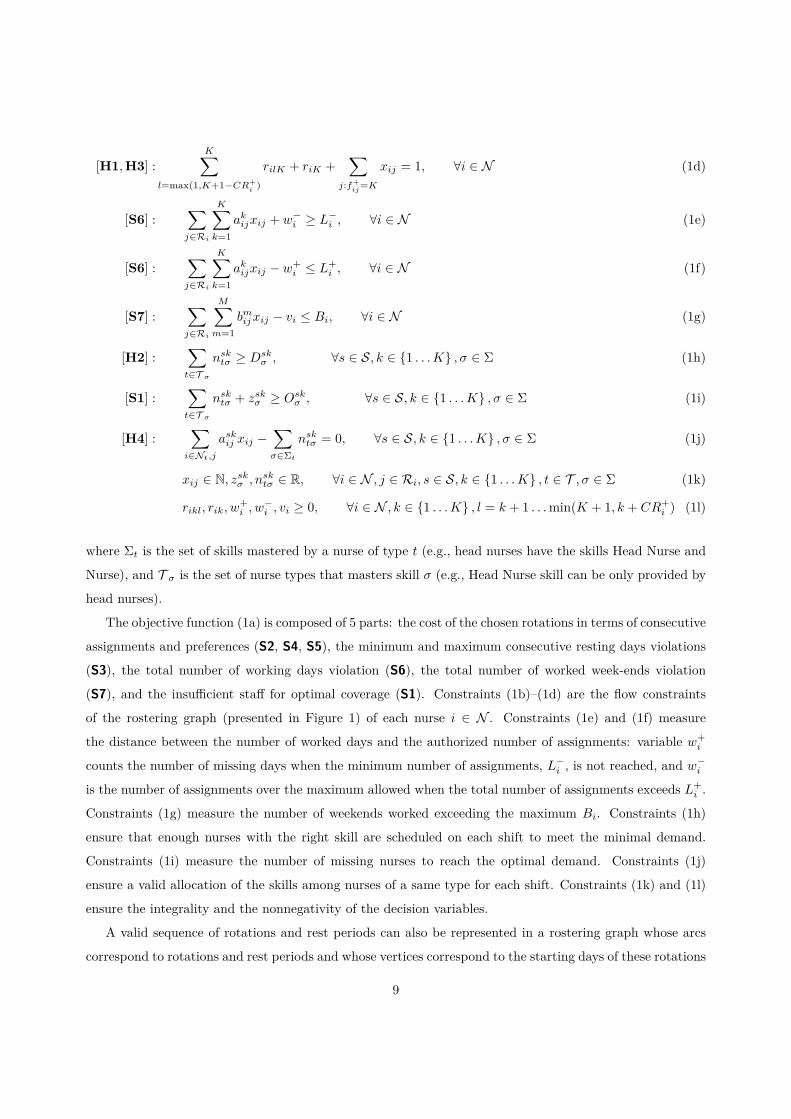
4.2.1. A primal-dual algorithm
Primal-dual algorithms for online optimization aim at building pairs of primal and dual solutions dy-
namically. At each stage, primal decisions are irrevocably made and the dual solution is updated so as to
remain feasible. The current dual solution drives the algorithm to better primal decisions by using those
dual values as multipliers in a Lagrangian relaxation. The goal is to obtain a pair of feasible primal and
dual solutions that satisfy the complementary slackness property at the end of the process.
We use a similar primal-dual algorithm to solve the online problem associated to Formulation (2). In
this dynamic process, we wish to sequentially solve a restriction of Formulation (2) to week m for all
stages m ∈ 1, . . . ,M with a view to reaching an optimal solution of the complete formulation. This
process raises an issue though: how can constraints (4c)-(4e) betaken into account in a restriction to a single
week? To achieve that goal, the primal-dual algorithm uses dual information from stage m to compute the
schedule of stage m+ 1 by solving the following Lagrangian relaxation of Formulation (2):
min∑j∈R
[ cj︸︷︷︸S1,S2,S3,S4,S5
+∑i∈N
(β+i − β
−i )aij︸ ︷︷ ︸
S6
+∑i∈N
γibij︸ ︷︷ ︸S7
]ym+1j (3a)
s.t.: [H1−H3] :∑j∈Cjm
ym+1j = 1 (3b)
ym+1j ∈ 0, 1, ∀j ∈ R (3c)
where β−i , β+i , γi ≥ 0 are multipliers respectively associated with constraints (2d) – (2f), and both con-
straints (2b) and (2c) that guarantee the feasibility of the weekly schedules are aggregated under Con-
straint (3b). More specifically, any new assignment for nurse i will be penalized with β−i − β+i and worked
week-ends will cost an additional γi. It is thus essential to set these multipliers to values that will drive the
computation of weekly schedules towards efficient schedules over the complete horizon. For this, we consider
the dual of the linear relaxation of Formulation (2):
maxM∑m=1
αm +∑i∈N
(L−i β−i − L
+i β
+i −Biγi) (4a)
s. t.: αm +∑i∈N
(aijβ−i − aijβ+i − bijγi)− δ
mj +
∑j′∈C−1
j
δm−1j′ ≤ cj , ∀j ∈ R,∀m [ymj ] (4b)
β−i ≤ c6, ∀i ∈ N [w−i ] (4c)
β+i ≤ c6, ∀i ∈ N [w+
i ] (4d)
γi ≤ c7, ∀i ∈ N [vi] (4e)
β+i , β
−i , γi, δ
mj ≥ 0, ∀j ∈ R,m ∈ 1 . . .M ,∀i ∈ N (4f)
13

where set C−1j contains all the schedules with which schedule j is compatible. Dual variables αm, δmj , β−i , β
+i
and γi are respectively associated with Constraints (2b), (2c), (2d), (2e), and (2f), and the variables δ0j are
set to zero to obtain a unified formulation. The variables in brackets denote the primal variables associated
to these dual constraints. At each stage, the primal-dual algorithm sets the values of the multipliers so
that they correspond to a feasible and locally-optimal dual solution, and uses this solution as Lagrangian
multipliers in Formulation (2). Another point of view is to consider the current primal solution at stage m
as a basis of the simplex algorithm for the linear relaxation of Formulation (2). The resolution of stage m+1
corresponds to the creation of a new basis: Formulation (3) seeks a candidate pivot with a minimum reduced
cost according to the associated dual solution.
Not only does the choice of dual variables drives the solution towards dual feasibility, but it also guar-
antee that complementary conditions between the current primal solution at stage m and the dual solution
computed for stage m + 1 are satisifed. In the computation of a dual solution, the variables αm and δmj
do not need to be explicitly considered, because they will not be used in Formulation (3). What is more,
focusing on stage m, the only dual constraints that involve αm and δmj (4b), can be satisfied for any value
of β−i , β+i and γi by setting δmj = 0,∀j ∈ R, and
αm = minj∈Rcj −
∑i∈N
(aij β−i − aij β+i − bij γi).
Observe that the expression of the objective function of Formulation (2) ensures that the only schedule
variable satisfying ymjm > 0 will be such that jm ∈ argminj∈Rcj −∑i(aijβ
−i − aijβ
+i − bijγi), so comple-
mentarity is achieved.
To set the values of β−i , β+i and γi, we first observe that complementary conditions are satisfied if
β−i =
c6 if∑j,m aijy
mj < L−i
0 otherwiseβ+i =
c6 if∑j,m aijy
mj ≥ L
+i
0 otherwiseγi =
c7 if∑j,m bijy
mj ≥ Bi
0 otherwise
Since the history of the nurses are initialized with zero assignment and week-end worked, we initially set
β−i = c6 and β+i = γi = 0 to satisfy complementarity. We then perform linear updates at each stage m,
using the characteristics of the schedule jm chosen for the corresponding week:
β−i = max(
0, β−i − c6amijmL−i
), β+
i = min(c6, β
+i + c6
amijmL+i
), γi = min
(c7, γi + c7
bmijmBi
).
These updates do not maintain complementarity at each stage but allow for a more balanced penaliza-
tion of the number of assignments and worked week-ends. The variations of β−i , β+i and γi ensure that
constraints (2b) remain feasible for the previous stage, even though complementarity may be lost.
In most theoretical descriptions of the online primal-dual algorithm, the authors use non-linear updates
14
to be able to derive a competitive-ratio. However, no competitive-ratio is sought by this approach and linear
updates are easier to design. Non-linear updates could be investigated in the future.
Algorithm 2 summarizes the primal-dual algorithm. It estimates the impact of a chosen schedule on the
global soft constraints through their dual variables. As it is, it gives mixed results in practice. The reason
is that the information obtained through the dual variables does not describe precisely the real problem. At
the beginning of the algorithm, the value of the dual variables drives the nurses to work as much as possible.
Consequently, the nurses work too much at the beginning and cannot cover all the necessary shifts at the
end of the horizon. Furthermore, the expected impact of the filtering constraints (2c) are totally ignored in
that version. Namely, the shift type succession constraints H3 imply many feasibility issues at the border
between two weeks as Formulation (2) is solved sequentially with this primal-dual algorithm. The following
two sections describe how this initial implementation is adapted to cope with these issues.
Algorithm 2: Primal-dual algorithmβ−i = c6, β
+i = γi = 0,∀i ∈ N
for each stage m doSolve Formulation (3) with a deterministic algorithmUpdate β−i = max
(0, β−i − c6
amijmL−i
),∀i ∈ N
Update β+i = min
(c6, β
+i + c6
amijmL+i
),∀i ∈ N
Update γi = min(c7, γi + c7
bmijmBi
),∀i ∈ N
end for
4.2.2. Sampling a second week demand for feasibility issues
Preliminary results have shown that Algorithm 2 raises feasibility issues due to constraints H3 on forbid-
den shift successions between the last day of one week and the first day of the following one. In other words,
there should be some way to capture border effects during the computation of a weekly schedule. Instead
of solving each stage over one week, we solve Formulation (3) over two weeks and keep only the first week
as a solution of the current stage. The compatibility constraints (2c) between stages m and m+ 1 are now
included in this two-weeks model. In this approach, the data of the first week is available but no data of
future stages is available. The demand relative to the next week is thus sampled as described in Section 4.4.
The fact that the schedule is generated for stages m and m+ 1 ensures that the restriction to stage m ends
with assignments that are at least compatible in this scenario, thus increasing the probability of building a
feasible schedule over the complete horizon.
Furthermore, for two different samples of following week demand, the two-weeks version of Formula-
tion (3) should lead to two different solutions for the current week. As a consequence, we can solve the
model several times to generate different candidate schedules for stage m. As described in Algorithm 1, we
use this property to generate new candidates until time limit is reached.
15

4.2.3. Global bounds to reduce staff shortages
Preliminary results have also shown that Algorithm 2 creates many staff shortages in the last weeks.
Our intent is thus to bound the number of assignment and worked weekends in the early stages to avoid
the later shortages. The naive approach is to resize constraints (2d)-(2f) proportionally to the length of
the demand considered in Formulation (3) (i.e., two weeks in our case). However, it can be desirable to
allow for important variations in the number of assignments to a given nurse from one week to another, and
even from one pair of weeks to another. Stated otherwise, it is not optimal to build a schedule that can
only draw one or two weeks-long patterns as would be the case for less constrained environments. A simple
illustration arises by considering the constraints on the maximum number of worked weekends. To comply
with these constraints, no nurse should be working every weekend and, because of restricted staff availability,
it is unlikely that a nurse is off every weekend. Coupled with the other constraints, this results necessarily
in complex and irregular schedules. Consequently, bounding the number of assignments individually would
discard valuable schedules.
Instead, we propose to bound the number of assignments and worked weekends for sets of similar nurses
in order to both stabilize the total number of worked days within this set and allow irregularities in the
individual schedules. We choose to cluster nurses working under the same work contract, because they share
the same minimum and maximum bounds on their soft constraints. Hence, for each stage m, we add one set
of constraints similar to (2d)-(2f) for each contract. In the constraints associated with contract κ ∈ Γ, the
left hand-sides are resized proportionally to the number of nurses with contract κ and the number of weeks
in the demand horizon. Let Lm−κ , Lm+κ , and Bmκ be respectively the minimum and maximum total number
of assignments, and the maximum total number of worked weekends over the two-weeks demand horizon for
the nurses with contract κ. We define these global bounds as:
• Lm−κ = 7 ∗ 2M−m+1
∑i:κi=κ max(0, L−κi −
∑m′<mm′=1
∑j aijy
m′
j ),
• Lm+κ = 7 ∗ 2
M−m+1∑i:κi=κ max(0, L+
κi −∑m′<mm′=1
∑j aijy
m′
j ),
• Bmκ = 2M−m+1
∑i:κi=κ max(0, Bκi −
∑m′<mm′=1
∑j bijy
m′
j ),
where κi is the contract of a nurse i.
Finally, the objective (3a) is modified to take into account the new slack variables wm−κ , wm+κ , vmκ as-
sociated to the new soft constraints. The costs of these slack variables is set to make sure that violations
of the soft constraints are not penalized more than once for an individual nurse. For instance, instead of
counting the full cost c6 for variable wm+κ , we compute its cost as (c6 − maxi|κi=κ(β+
i )). This guarantees
that an extra assignment is never penalized with more than c6 for any individual nurse. The cost of the
variables wm+κ and vmκ have been modified in the same way for analogous reasons.
Formulation (5) summarizes the final model used for the generation of the schedules. We recall that the
16

variables ymj are now selecting a schedule j which covers a two weeks demand, and that this formulation is
in fact solved by a branch-and-price algorithm that selects rotations instead of weekly schedules.
min∑j∈R
[cj +
∑i∈N
((β+i − β
−i )aij + γib
mij
)]ymj
+∑κ∈Γ
[(c6 − max
i:κi=κ(β−i ))wm−κ + (c6 − max
i:κi=κ(β+i ))wm+
κ ) + (c7 − maxi:κi=κ
(γmi ))vmκ )]
(5a)
s.t.: [H1,H2,H3,H3] :∑j∈R
ymj = 1, (5b)
[S6] :∑i:κi=κ
∑j∈R
aijymj + wm−κ ≥ Lm−κ , ∀κ ∈ Γ (5c)
[S6] :∑i:κi=κ
∑j∈R
aijymj + wm+
κ ≤ Lm+κ , ∀κ ∈ Γ (5d)
[S7] :∑i:κi=κ
∑j∈R
bijymj − vmκ ≤ Bmκ , ∀κ ∈ Γ (5e)
ymj ∈ 0, 1, ∀j ∈ R (5f)
wm−κ , wm+κ , vmκ ≥ 0, ∀κ ∈ Γ (5g)
To conclude, Formulation (5) allows to anticipate the impact of a schedule on the future through two
mechanisms: the problem is solved over two weeks to diminish the border effects that may lead to infeasibility,
and the costs are modified to globally limit the penalties due to constraints S6 and S7. Furthermore, this
formulation can generate different schedules fort the first week by considering different samples for the second
week demand.
4.3. Evaluating candidate schedules
In the spirit of the SAA, the first-week schedules generated by Formulation (5) are evaluated to be
ranked. The evaluation should measure the expected impact of each schedule on the global solution (i.e.,
over M weeks). This impact can be measured by solving a NSP several times over different sampled demands
for the remaining weeks.
Let Ωm be the set of scenarios of future demands for weeks m+ 1, . . . ,M , and assume that a schedule j
has been computed for week m. To evaluate schedule j, we wish to solve the NSP for each sample of future
demand ω ∈ Ωm by using j to set the initial history of the NSP. Denoting V mjω the value of the solution,
we can infer that the future cost cmjω of schedule j in scenario ω is equal to cj + V mjω : the actual cost of
the schedule plus the resulting cost for scenario ω. Then, a score that takes into account all the future
costs (cmjω)ω∈Ωm of a given schedule j is computed. Several functions have been tested and preliminary
17

results have shown that the expected value was producing the best results. Finally, the schedule jm with
the best score is retained.
However, computing the value V mjω raises two main issues. First, the NSP is an integer program for which
it can be time-consuming to even find a feasible solution. We thus use the linear relaxation of this problem
as an estimation of the future cost. This simplification decreases drastically the computational time, but
still can detect feasibility issues at the border between weeks m and m+ 1. The second issue is that over a
long time horizon, even the linear relaxation of the NSP cannot be solved in sufficiently small computational
time. We thus restrict the evaluation to scenarios of future demands that are at most two weeks long. More
specifically, the scenarios are one week-long for the penultimate stage (M − 1) and two weeks long for the
previous stages. We observed that this restriction allows to keep the solution time short enough while giving
a good measure of the impact of the schedule j on the future.
To summarize, the value V mjω is computed by solving the linear relaxation of Formulation (1) for a two-
week demand ω, and the initial state is set by using the schedule j. Finally, the parameters L−i , L+i , and
Bi are proportionally resized over two weeks, as follows.
• L(m+1)−i = b7 ∗ 2
M−m max(0, L−i −∑mm′=1
∑j a
m′
ij ym′
j )c;
• L(m+1)+i = d7 ∗ 2
M−m max(0, L+i −
∑mm′=1
∑j a
m′
ij ym′
j )e;
• Bm+1i = d 2
M−m max(0, Bi −∑mm′=1
∑j bm′
ij ym′
j )e.
As already stated, the number of evaluation scenario included in Ωm is kept low (e.g., |Ωm| = 5) to meet
the requirements in computational time. These scenarios are sampled as described in the next section.
4.4. Sampling of the scenarios
The competition data does not provide any knowledge about past demands, potential probability distri-
butions of the demand, nor any other type of information that could help for sampling scenarios of demand.
It is thus impossible to build complex and accurate prediction models for the future demand. At a given
stage m, the algorithm has absolutely no knowledge about the future realizations of the demand, so the
sampling can only be based on the current and past observations of the weekly demands on stages 1 to m.
To build scenarios of future demand, we simply perturb these observations with some noise that is uniformly
distributed within a small range (typically one or two nurses) and randomly mix these observations (e.g.,
pick the Monday of one observation and the Tuesday from another one). The future preferences are not
sampled in the scenarios, because they cannot lead to an infeasible solution, they do not induce border
effects, and they have small costs when compared to the other soft constraints. The goal of the sampling
method is only to obtain some diversity in the scenarios used to generate different candidate schedules and
in those used to evaluate the candidate schedules. Assuming that the demands will not change dramatically
from one week to another, this allows for additional robustness and efficiency in many situations.
18

4.5. Summary of the primal-dual-based sample average approximation
Algorithm 3 provides a detailed description of the overall algorithm we submitted to the INRC–II.
It generates several schedules with a primal-dual algorithm and evaluates them over a set Ωm of future
demands. The evaluation step increases the probability of selecting a globally feasible schedule, that has
already been feasible for several resolutions of the linear relaxation of Formulation (1). The performances
of this algorithm are discussed in Section 5.
Algorithm 3: A primal-dual-based sample average approximationβ−i = c6, β
+i = γi = 0,∀i ∈ N
for each stage m = 1 . . .M − 1 doInitialize the set of candidate schedules of stage m: Sm = ∅Initialize the generation model using the chosen schedule of the previous stage m− 1 (i.e., set theinitial state)Sample a set Ωm of future demands for the evaluationwhile there is enough computational time do
Sample a second week demand for the generationSolve Formulation (5) with a deterministic algorithm to build a two-weeks schedule (j1, j2)Store the schedule of the first week: Sm := Sm ∪ j1Initialize the evaluation model with schedule j1 (i.e., set the initial state)for each demand ω ∈ Ωm do
Compute the value V mjω as the optimal value of the linear relaxation of Formulation (1) over twoweeks if m < M − 1, and one week otherwise
end forend whileChoose the schedule jm with the best average evaluation costUpdate the dual variables as in Algorithm 2
end forCompute the best schedule for the last stage M with the given computational time
5. Experimentations
This section presents the results obtained at the INRC–II. The competition was organized in two rounds.
In the selection round, each team had to submit their best results on a benchmark of 28 instances that were
available to the participants before submitting the codes. The organizers then retained the best eight teams
for the final round where they tested the algorithms against a new set of 60 instances. The algorithm
described above ranked second in both rounds.
The instances used during each round are summarized in Tables 3 and 4. They range from relatively
small instances (35 nurses over 4 weeks) to really big ones (120 nurses over 8 weeks) that are very difficult to
solve even in a static setting [13]. The algorithms of the participants all had the same limited computational
time to solve each stage (depending on the number of nurses and on the computer used for the tests1). The
1The computational times are given for a linux computer Intel(R) Xeon(R) X5675 @ 3.07GHz with 8 Go of available memory.
19

solution obtained at each stage was used as an initial state for the schedule of the following week. If an
algorithm reached an infeasible schedule, the iterative process was stopped. The final rank of each team was
computed as the average rank over all the instances.
Number of nurses30 40 50 60 80 100 120
Number of weeks 4 2 2 2 2 2 2 28 2 2 2 2 2 2 2
Computational time per week (s)1 35 60 90 120 150 240 300
Table 3: Instances used for the selection
Number of nurses35 70 110
Number of weeks 4 10 10 108 10 10 10
Computational time per week (s)1 45 150 270
Table 4: Instances used for the final
In this section, we will focus our discussion on the quality of the results obtained with our algorithm.
More details about the competition and the results can be found on the competition website: http://
mobiz.vives.be/inrc2/.
5.1. Algorithm implementation
Algorithm 3 depends on how future demands are sampled, on the number of scenarios used for the
evaluation, and last but not least, on the scheduling software.
The algorithm uses only five scenarios of future demands for the evaluation. It must indeed divide the
short available computational time between the generation and the evaluation of the schedules. The first
step aims at computing the best schedule according to the current demand while the second step seeks a
robust planning that yields promising results for the following stages (high probability to remain feasible and
near-optimal). In order to generate several schedules (at least two) within the granted computational time,
the number of demand scenarios must remain small. Moreover, since the demand scenarios we generate are
not based on accurate data, but only on a learned distribution, there is no guarantee that a larger number
of scenarios would provide a better evaluation. In fact, we tested different configurations (3 to 10 scenarios
used for the evaluation), and they all gave approximately the same results (the best results were obtained
for 4 to 6 scenarios).
The code is publicly shared on a Git repository [14]. The scheduling software is implemented in C++
and is based on the branch-cut-and-price framework of the COIN-OR project, BCP. The choice of this
framework is motivated by the competition requirement of using free and open-source libraries. The pricing
problems are modeled as shortest paths with resource constraints and solved with the Boost library. The
20
solution algorithm is not parallelized and it uses the branching strategy ‘two dives’ described in [13]. This
strategy ‘dives’ two times in the branching tree and keeps the best feasible solution. If no solution is found
after two dives (which was never the case), the algorithm continues until it reaches either the time limit or
a feasible solution.
5.2. Selection instances
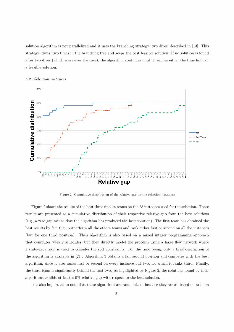
Figure 2: Cumulative distribution of the relative gap on the selection instances
Figure 2 shows the results of the best three finalist teams on the 28 instances used for the selection. These
results are presented as a cumulative distribution of their respective relative gap from the best solutions
(e.g., a zero gap means that the algorithm has produced the best solution). The first team has obtained the
best results by far: they outperform all the others teams and rank either first or second on all the instances
(but for one third position). Their algorithm is also based on a mixed integer programming approach
that computes weekly schedules, but they directly model the problem using a large flow network where
a state-expansion is used to consider the soft constraints. For the time being, only a brief description of
the algorithm is available in [21]. Algorithm 3 obtains a fair second position and competes with the best
algorithm, since it also ranks first or second on every instance but two, for which it ranks third. Finally,
the third team is significantly behind the first two. As highlighted by Figure 2, the solutions found by their
algorithms exhibit at least a 9% relative gap with respect to the best solution.
It is also important to note that these algorithms are randomized, because they are all based on random
21

sampling of future demands. For the first phase of the competition, the participants had to provide the
random seeds they used to obtain their results. During the second phase, the organizers executed the code
of each team ten times with different arbitrary random seeds on each instance.
Figure 3: Distribution of the objective value for the selection instances
Figure 3 shows the distribution of the objective value for 180 observations of the solution of an instance
with 80 nurses over 8 weeks using Algorithm 3. The values of the solution are within a [−6%,+7%] range.
Because of these variations, we run the algorithm many times on each of the instances used for the selection
to submit only the best ones and increase our chance of qualification. Most teams must have used the same
technique, since the ranking between the selection and the final rounds did not really change.
5.3. Final instances
The final results respect the same ranking as the one obtained after the selection. However, these
comparisons are more fair, since the results were computed by the organizers, so that the teams were not
able to select the solutions they submitted. This configuration evaluates in a better way the proposed
algorithms, and especially their robustness. The organizers have even run 10 times the algorithms on each
of the 60 final instances, and have thus compared the proposed software over 600 tests.
22

Figure 4: Cumulative distribution of the relative gap on the final instances
Figure 4 presents the relative gaps obtained on the final instances. The two first teams are really close
and their algorithms highlight two distinct features of the competition. The winning team’s algorithm builds
the best schedules for about 65% of the instances, but our algorithm appears to be more robust. We indeed
able produced a feasible schedule in every test but one, while winners could not build a feasible schedule in
5% of the cases (i.e., 34 tests). This comparison also highlights the balance that needs to be found between
the time spent in the generation of the best possible schedules and their evaluation, since this second phase
provides a measure of their robustness to future demands.
Figure 5 shows the cumulative distribution of the relative gap of the winning team solutions from ours as
a function of the number of nurses. It is clear that once the instances exceed a certain size (i.e., 110 nurses),
the quality of the solution of the winning team decreases. Indeed, in [21], the winning team comments
that their algorithms was simply unable to find feasible integer solutions for some week demands of these
instances, showing that the method experiments difficulties in scaling up. Furthermore, this algorithm was
also not able to find feasible solutions for an important number of the small instances (i.e., 35 nurses). As a
possible explanation, we have observed that it is more difficult to find feasible solutions for these instances,
because they leave less flexibility for creating the schedules, i.e., because the hard constraints of the MIP
are tighter. Stated otherwise, the proportion of feasible schedules that meet the minimum demand is much
smaller for the smallest instances used in the competition.
23

Figure 5: Cumulative distribution of the relative gap as a function of the number of nurses
6. Conclusions
This article deals with the nurse scheduling problem as described in the context of the international
competition INRC–II. The objective is to sequentially build, week by week, the schedule of a set of nurses
over a planning horizon of several weeks. In this dynamic process, the schedule computed for a given week is
irrevocably fixed before the demand and the preferences for the next week are revealed. The main difficulty
is to correctly handle the border effects between weeks and the global soft constraints to compute a feasible
and near-optimal schedule for the whole horizon.
Our main contribution is the design of a robust online stochastic algorithm that performs very well over
a wide range of instances (from 30 to 120 nurses over a four or eight weeks horizon). The proposed algorithm
embeds a primal-dual algorithm within a sample average approximation. The primal-dual procedure gen-
erates candidate schedules for the current week, and the sample average approximation allows to evaluate
each of them and retain the best one. The resulting implementation is shared on a public repository [14]
and builds upon an open source static nurse scheduling software.
The designed algorithm won second prize in the INRC–II competition. The results show that, although
this procedure does not compute the best schedules for a majority of instance, it is the most robust one.
Indeed, it finds feasible solutions for almost every instance of the competition while providing high-quality
schedules.
24

Despite the limits of this algorithm, our intent with this article is to present the exact implementation
that has been submitted to the competition. There is place for improvements that could be developed in the
future. For instance, the primal-dual algorithm could be enhanced with non-linear updates, new features
recently developed in the static nurse scheduling software could be tested, or the bounding constraints added
in the primal-dual algorithm could be refined.
References
[1] N. Bauerle and U. Rieder. Markov Decision Processes with Applications to Finance. Springer Science & Business Media,
2011.
[2] R. W. Bent and P. Van Hentenryck. Scenario-based planning for partially dynamic vehicle routing with stochastic
customers. Operations Research, 52(6):977–987, 2004.
[3] J. R. Birge and F. Louveaux. Introduction to Stochastic Programming. Springer Series in Operations Research and
Financial Engineering. Springer, New York, NY, USA, 2nd edition, 2011. doi: 10.1007/978-1-4614-0237-4.
[4] N. Buchbinder. Designing Competitive Online Algorithms via a Primal-Dual Approach. PhD thesis, Technion, 2008.
[5] E. K. Burke, P. De Causmaecker, G. V. Berghe, and H. Van Landeghem. The state of the art of nurse rostering. Journal
of Scheduling, 7(6):441–499, 2004. ISSN 1099-1425. doi: 10.1023/B:JOSH.0000046076.75950.0b.
[6] S. Ceschia, N. T. T. Dang, P. De Causmaecker, S. Haspeslagh, and A. Schaerf. The second international nurse rostering
competition. In PATAT 2014: Proceedings of the 10th International Conference of the Practice and Theory of Automated
Timetabling, pages 554–556, 2014.
[7] B. T. Denton, A. J. Miller, H. J. Balasubramanian, and T. R. Huschka. Optimal allocation of surgery blocks to operating
rooms under uncertainty. Operations research, 58(4-Part-1):802–816, 2010. doi: 10.1287/opre.1090.0791.
[8] G. Desaulniers, J. Desrosiers, and M. M. Solomon. Column generation, volume 5. Springer Science & Business Media,
2006.
[9] S.-E. Fleten and T. K. Kristoffersen. Short-term hydropower production planning by stochastic programming. Computers
& Operations Research, 35(8):2656 – 2671, 2008. ISSN 0305-0548. doi: http://dx.doi.org/10.1016/j.cor.2006.12.022. URL
http://www.sciencedirect.com/science/article/pii/S0305054806003224. Queues in Practice.
[10] A. J. Kleywegt, A. Shapiro, and T. Homem-de Mello. The sample average approximation method for stochastic discrete
optimization. SIAM Journal on Optimization, 12(2):479–502, 2002. doi: 10.1137/S1052623499363220.
[11] A. J. Kleywegt, A. Shapiro, and T. Homem-de Mello. The sample average approximation method for stochastic discrete
optimization. SIAM Journal on Optimization, 12(2):479–502, 2002. doi: 10.1137/S1052623499363220.
[12] A. Legrain, M.-A. Fortin, N. Lahrichi, and L.-M. Rousseau. Online stochastic optimization of radiotherapy patient
scheduling. Health Care Management Science, 3(3):1–14, 2014.
[13] A. Legrain, J. Omer, and S. Rosat. A rotation-based branch-and-price approach for the nurse scheduling problem, 2017.
URL https://hal.archives-ouvertes.fr/hal-01545421.
[14] A. Legrain, J. Omer, and S. Rosat. Dynamic nurse scheduler. https://github.com/legraina/DynamicNurseScheduler.
git, 2017.
[15] A. Nagesh. Nurses could go on strike for the first time in british history. http://metro.co.uk/2017/05/14/
nurses-could-go-on-strike-for-the-first-time-in-british-history-6636606/, 2017. Accessed: 2017-05-23.
[16] C. Novoa and R. Storer. An approximate dynamic programming approach for the vehicle routing problem with stochastic
demands. European Journal of Operational Research, 196(2):509–515, 2009.
[17] J. Patrick, M. L. Puterman, and M. Queyranne. Dynamic multipriority patient scheduling for a diagnostic resource.
Operations Research, 56(6):1507–1525, 2008.
25

[18] W. B. Powell. Approximate Dynamic Programming: Solving the Curses of Dimensionality. John Wiley & Sons, 2007.
[19] M. L. Puterman. Markov Decision Processes: Discrete Stochastic Dynamic Programming. John Wiley & Sons, 2014.
[20] A. Robbins. We need more nurses. http://www.nytimes.com/2015/05/28/opinion/we-need-more-nurses.html?_r=0,
2015. Accessed: 2017-05-23.
[21] M. Romer and T. Mellouli. A direct MILP approach based on state-expanded network flows and anticipation for multi-
stage nurse rostering under uncertainty. In Proceedings of the 11th International Confenference on Practice and Theory
of Automated Timetabling (PATAT-2016), 2016.
[22] P. Van Hentenryck and R. Bent. Online Stochastic Combinatorial Optimization. The MIT Press, 2009.
26


