
Retrospective Theses and Dissertations Iowa State University Capstones, Theses andDissertations
1-1-2001
Analysis and interpretation of roadway weather datafor winter highway maintenanceDavid Scott KnollhoffIowa State University
Follow this and additional works at: https://lib.dr.iastate.edu/rtd
This Thesis is brought to you for free and open access by the Iowa State University Capstones, Theses and Dissertations at Iowa State University DigitalRepository. It has been accepted for inclusion in Retrospective Theses and Dissertations by an authorized administrator of Iowa State University DigitalRepository. For more information, please contact [email protected].
Recommended CitationKnollhoff, David Scott, "Analysis and interpretation of roadway weather data for winter highway maintenance" (2001). RetrospectiveTheses and Dissertations. 18750.https://lib.dr.iastate.edu/rtd/18750

Analysis and interpretation of roadway weather data
for winter highway maintenance
by
David Scott Knollhoff
A thesis submitted to the graduate faculty
in partial fulfillment of the requirements for the degree of
MASTER OF SCIENCE
Major: Meteorology
Major Professors: Eugene S. Takle and William A. Gallus, Jr.
Iowa State University
Ames, Iowa
2001

ll
Graduate College Iowa State University
This is to certify that the Master' s thesis of
David Scott Knollhoff
has met the thesis requirements of Iowa State University
Signatures have been redacted for privacy

111
DEDICATION
I would like to dedicate this project to Mr. Arthur Moser. Arthur was my junior college
mathematics teacher in Illinois during the early 1990s. He is my beloved friend, my spiritual
mentor, and my brother in Christ. I can ' t even begin to count the hours of free mathematical aid
and spiritual guidance he gave to me! He not only helped me to pursue my goal of becoming a
professional meteorologist, but he taught me to pursue my goal in such a way that my Lord
Jesus Christ would be glorified through all my audible words and through my daily interactions
with others (Colossians 3: 17) that I would meet along the path of life. I look forward to the day
when I can give back to someone the gift that I have been given by God- an ordinary man with
extraordinary wisdom to share. Thanks, Mo. I love you, and you are in my thoughts daily.

IV
TABLE OF CONTENTS
LIST OF FIGURES
LIST OFT ABLES
ABSTRACT
CHAPTER 1. INTRODUCTION
CHAPTER 2. LITERATURE REVIEW 2.1. Winter road surface temperature and road condition analyses 2.2. Frost formation on roadways and bridges
CHAPTER 3. PAVEMENT TEMPERATURE ANALYSIS 3.1. Introduction 3.2. Data 3.3. RWIS locations and site characteristics 3.4. Procedure 3.5 . Analysis of pavement temperatures at RWIS sites in Des Moines
3 .5 .1. Pavement temperature differences 3.5.2. Cooling rates 3.5.3 . Mean lag times
3.6. Analysis of pavement temperatures at RWIS sites in Cedar Rapids 3.6.l. Pavement temperature differences 3.6.2. Cooling rates 3.6.3. Mean lag times
3.7. Summary
CHAPTER 4. PAVEMENT FROST ANALYSIS ON IOWA BRIDGE DECKS 4.1. Introduction 4.2. Data
4.2. l. RWIS data 4.2.2. Pavement frost observations 4.2.3. Potential errors
4.3. Procedure 4.3.l. Linear interpolation 4.3.2. Frost formation on pavement surfaces 4.3.3. Basic assumptions
4.4. Frost accumulation model 4.5. Model results 4.6. Binary contingency table methodology, results, and discussion
4.6.1. Methodology 4.6.2. Results 4.6.3. Discussion
4.7. Forecast accuracy and decision criterion 4.7.l. Signal detection theory 4.7.2. Relative operating characteristic curves 4.7.3. Area under the ROC curves
4.8. Logistic regression model 4.9. Summary
YI
Yll
Vlll
l
3 3 5
7 7 7 9
10 12 12 14 18 19 19 20 22 23
25 25 26 26 26 26 27 27 27 28 30 32 33 33 34 36 39 39 40 40 43 44

v
CHAPTER 5. CONCLUSIONS 47
APPENDIX A. DERIVATION OF FROST ACCUMULATION MODEL 49
APPENDIX B. FROST ACCUMULATION MODEL (FAM2000) SOURCE CODE 51
APPENDIX C. POSITIVE MODEL FROST ACCUMULATION CASES 64
APPENDIX D. CONTINGENCY TABLES FOR THE VARIO US FROST DEPTHS 68
REFERENCES 70
ACKNOWLEDGEMENTS 73
BIOGRAPHICAL SKETCH 74

VI
LIST OF FIGURES
Figure 1. Southwest Des Moines roadway pavement temperatures for the 96/97 winter season. 8
Figure 2. DSM RWIS pavement temperatures (01113/97). 13
Figure 3. Downtown RA cooling rates in Des Moines for the different cloud cover classifications. 17
Figure 4. Conditions accompanying frost formation. 29
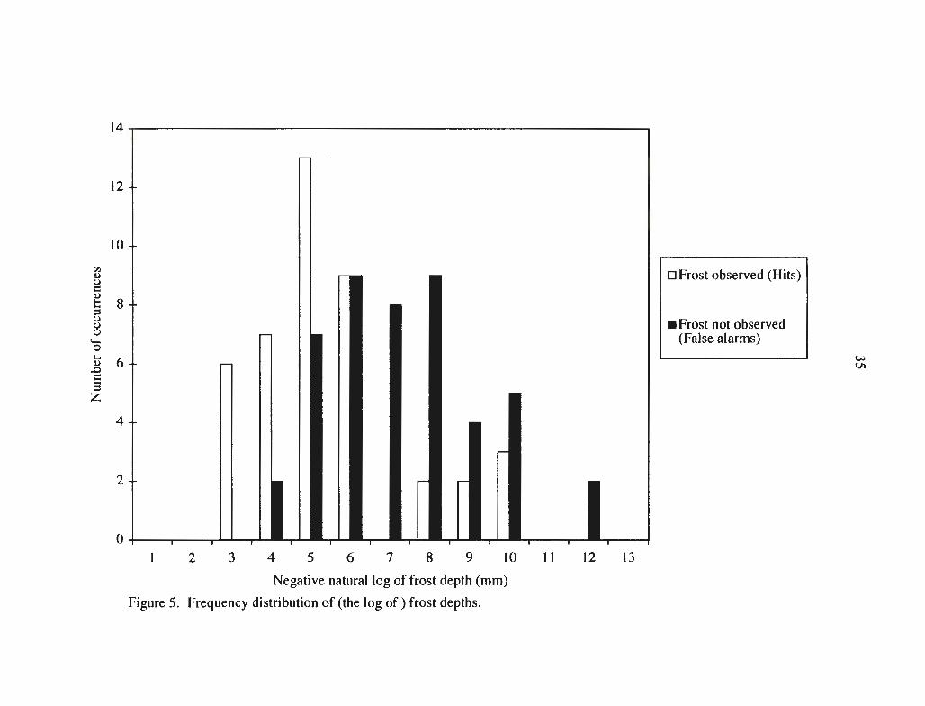
Figure 5. Frequency distribution of (the log of) frost depths. 35
Figure 6. Effect on Hand FAR of various thresholds. 37
Figure 7. The set of black dots defines the ROC curve using point estimates of H and FAR! for the various threshold frost depths. 41
Figure 8. The set of black dots defines the ROC curve using point estimates of H and FAR2 for the various threshold frost depths. 42
Figure 9. The probability (p) that IaDOT personnel will see frost for a predicted frost depth. 45
Vll
LIST OF TABLES
Table 1. RWIS sites and sensor locations. 9
Table 2. Average and standard deviation [in brackets] of ~T (°C) in Des Moines. 14
Table 3. Average and standard deviation [in brackets] values of cooling rates (°C h" 1)
for Des Moines. 15
Table 4. Mean downtown lag times (h) in Des Moines. 18
Table 5. Average and standard deviation [in brackets] of ~T (°C) in Cedar Rapids. 20
Table 6. Average and standard deviation [in brackets] values of cooling rates (°C h" 1)
for Cedar Rapids. 21
Table 7. Mean downtown lag times (h) in Cedar Rapids. 23
Table 8. Conditions for frost deposition. 28
Table 9. Binary contingency table. 33
Table 10. SDT calculations with FARl. 38
Table 11. SDT calculations with FAR2. 38
Table 12. SDT definitions. 40

viii
ABSTRACT
Formation of ice and frost on pavement surfaces presents a potential hazard to the
motoring public in cold climates. Pavement temperatures are not measured routinely by the
National Weather Service and are not part of public forecasts of winter conditions, but highway
maintenance personnel must make frost suppression and anti-icing decisions based on
expectations of future pavement temperatures. The Road Weather Information System
measures pavement, air, and dew point temperatures, pavement conditions, and wind data at
numerous locations in the state of Iowa and reports the data in real-time to maintenance offices.
The surface and near-surface data from the road weather system were analyzed to develop
winter weather forecast procedures to compliment anti-icing techniques already practiced within
the Iowa Department of Transportation.
Nocturnal pavement temperatures as reported by temperature sensors located in and
near Des Moines and Cedar Rapids were analyzed under different classifications of cloud cover
and for seasonal variations. Results show that the urban pavement temperatures near both Des
Moines and Cedar Rapids are generally higher than rural pavement temperatures under different
sky conditions. The heat island impact on surface temperatures in Des Moines was found to be
slightly larger than that of Cedar Rapids. Pavement temperature cooling patterns differed
among the months analyzed, and the roadways had different cooling characteristics compared to
the bridge decks.
A model based on simple concepts of moisture flux to the surface was developed that
uses current road weather data and forecasts of dew-point temperature, air temperature, surface
temperature, and wind speed to calculate frost accumulation on bridge decks in Iowa. The
analysis showed that the model has sufficient accuracy to be used as an operational tool to
forecast bridge deck frost. A logistical regression procedure was developed to determine the
probability that a maintenance worker will observe frost for a given calculated frost depth.

l
CHAPTER 1. INTRODUCTION
From late autumn through early spring, the formation of frost on roadways and bridges
is a hazard to motorists in Iowa. Consequently, the Iowa Department of Transportation
(IaDOT) suppresses frost formation . IaDOT maintenance personnel receive site-specific road
weather forecasts to warn them on the timing details of frost events. Highway maintenance
personnel use anti-icing and deicing techniques to battle frost formation based on the prediction
of future road surface temperatures (RSTs) and road surface conditions (RSCs) provided in the
road weather forecasts . In addition to site-specific road weather forecasts, IaDOT maintenance
personnel use real-time road surface temperature and atmospheric temperature data measured
by Roadway Weather Information System (RWIS) sensors to monitor atmospheric and
pavement temperature trends. These data are collected and archived by the IaDOT.
In order to effectively combat the formation of frost on roadways and bridge decks
during the cold season, research on icy road events in Iowa is needed for many reasons. First,
Iowa RWIS stations are a fairly new addition to the IaDOT (late 1980s), and they have been
recently (1998) upgraded to a new statewide computer environment. Consequently, the ability
to access large amounts of RWIS data provides a valuable resource for numerous maintenance
decisions needed for Iowa roads during frost events. Real-time RWIS data are used to refine
the timing details of when to activate anti-icing and deicing procedures on paved roads.
Secondly, only one study (Takle, 1990) on pavement frost has been completed in Iowa. Takle
(1990) showed that a total of 2608 bridge and 1615 roadway frost observations occurred for the
winters from 1985 to 1989. He concluded that the number of bridge frost events ranges from
about 12 to 58, and that the number of roadway frost events varies from about 7 to 35 across
Iowa per year. This study revealed that frost frequently forms on paved surfaces in Iowa.
Thirdly, accurate prediction of winter RSTs and RSCs leads to economic, environmental and
human benefits (Thomes, 1989) notably safer roads, fewer anti-icing runs, less rust damage to
cars and bridges, and reduced waterway pollution. Lastly, the depth of frost accumulation and

2
the length of time frost is being deposited on paved surfaces are not easy variables to measure.
Thus, predictive models have been developed to predict RSTs and the absence or presence of
frost on bridges and roadway networks. Despite substantial improvements in understanding ice
formation on roadways (Bogren and Gustavsson, 1989), continued research is needed to
improve predictive models.
The goals of this study are to address this need for pavement temperature analyses in
Iowa during the laDOT winter maintenance season (October 15 through April 15) and to
improve the prediction of frost formation around Iowa. The first objective is accomplished
through analyses of nocturnal pavement temperature trends in Des Moines and Cedar Rapids.
The second portion of this thesis gives the results on the prediction of frost accumulation on
bridges by the use of a prognostic frost model and reports the results on the probability of a
human observing a predicted frost depth.

3
CHAPTER 2. LITERATURE REVIEW
Because the northern latitudes of North America and Europe experience frequent snow,
sleet, ice, and frost events during the cold season, the impacts of these conditions on highway
safety have stimulated numerous studies of road surface temperatures and winter road
conditions. RSTs and RSCs have been studied more heavily in Europe than anywhere else. In
part, this fact arises because Europe had a well established automated road weather network in
use by the mid 1980s, unlike the United States and Canada which began their RWIS networks
in the late 1980s. Recent European research has been focused on the controlling factors of road
surface temperature changes, on the prediction of RSTs and RSCs at site-specific road locations
and along road networks, and on the prediction of frost formation on pavement surfaces.
2.1. Winter road surface temperature and road condition analyses
Road temperatures can vary greatly across a road network, even within city limits
(Hewson and Gait, 1992). Topography is one of the most important factors controlling the
variation of RSTs along a road network. Shao et al. (1998) concluded that RSTs varied up to
10°C-12°C along a large mountainous road network having large variations in altitude in
Nevada. He also stated that, generally, a decrease of RST was observed with an increase in
altitude. A study by Bogren and Gustavsson (1991) showed that valley geometry affected
nocturnal pavement temperatures. They related the intensity of air temperature cold pools to the
width and depth of valleys in Sweden. They concluded that air temperature differences between
a valley and surrounding areas increased with increasing depth and width and that an increase in
cold air pool intensity of 1°C lowered the RST by 0.4°C during nocturnal hours. Gustavsson
(1990) described how the prevailing wind speed influenced pavement temperature variations in
the county of Skaraborg in Sweden. He found variations to be low with 2-m wind speeds
higher than 4 m s-1 to 5 m s-1• Another factor that affected nighttime RSTs was whether or not
the road surface was screened by objects (i.e., trees, buildings, hills) in the daytime (Bogren,
1991). He concluded that the RST differences between a screened site and an exposed site

4
during the day, due to the sky-view factor, influenced RST differences at those sites after
sunset.
Most prognostic roadway weather models in use today give site-specific forecasts where
RWIS sites are located. Real-time RWIS data from site-specific locations are used for
initializing model runs. Different RST models have been tested for site-specific locations in
western Europe (Rayer, 1987; Sass, 1992; Shao and Lister, 1996; Thornes and Shao, 1991).
Rayer (1987) developed one of the first operational RST numerical models which predicted
pavement temperatures for RWIS sites across the United Kingdom. His model included
schemes that considered the effects of clouds, rain, and changing solar declination. The United
Kingdom Meteorological Office first used the model in November 1986 as an advisory tool for
road maintenance engineers during the winter of 1986-1987. This study encouraged an
expansion of analyses on RSTs and the need for better prediction tools. Thornes and Shao
( 1991) looked at the interrelationships between RST and geographical road construction and
meteorological inputs using the Icebreak model (Shao, 1990). Sensitivity tests using the
Icebreak model showed that air temperature, cloud amount and cloud type were the most
important factors that influenced the variation of RSTs at road weather sites. They also
concluded that the influences of dew-point temperature, wind speed, and the thermal properties
of the pavement were small. Sass (1992) tested a prognostic road condition forecast model
developed at the Danish Meteorological Institute (DMI). This model was tested at a Danish
road station, where the model assumed that the road was fully exposed to sunshine. He found
that the best results in predicting RSTs and RSCs were obtained with detailed air temperature
and humidity analyses taken from radiosonde data. Because large model sensitivity was found
using atmospheric input data, Sass suggested that this model should be coupled to a realistic
atmospheric forecast model to get the best road surface results. The test results indicated that
the model could be used for high-quality RST forecasts up to 3 h. Shao and Lister (1996)
developed an automated road ice prediction model that provided short-term (up to 3 h) high-

5
accuracy forecasts of RSTs and RSCs. Their model is unique in that it is the only fully
automated physical road ice prediction model that requires no external meteorological input data
other than automatically collected sensor measurements of surface temperature, air temperature,
dew-point temperature, and wind speed from site-specific RWIS forecast sites. Results showed
that their technique is acceptable for short-term forecasts. They concluded that over 95% of 3-h
minimum temperature forecasts have an error of::; 2°C. However, model performance becomes
poorer as the forecast period gets longer.
RWIS sites monitor pavement temperature trends only at certain spots along roadway
networks. Other tools to monitor pavement temperature trends and conditions are used for
entire road networks. Thermal mapping is one widely used technique to record and quantify
patterns of RSTs along such networks. Thermal mapping is a useful tool to provide an
economic, easy, effective and accurate way to describe and display the actual spatial variations of
RSTs for road networks (Shao et al., 1997). A local climatological model (LCM) is another
tool used to predict RSTs and RS Cs along entire stretches of road. In summary, the authors
(Bogren et al., 1992; Gustavsson and Bogren, 1993) concluded that such tools as RWIS sites,
thermal mapping and LCMs enhanced the prediction of RSTs and RSCs.
2.2. Frost formation on roadways and bridges
Studies on the controlling factors of frost formation on roadways and bridges have
been completed by Gustavsson (1991) and Gustavsson and Bogren (1991) during warm-air
advection events. Gustavsson and Bogren (1990) concluded that the spatial distribution of
slipperiness in Sweden was dependent on two weather scenarios preceding the warm-air
advection. First, if clear and calm conditions existed before the advection event, large local
temperature differences due to variations of topography highly influenced how rapidly frost
formed. Considerable time differences for the onset of slippery conditions between adjacent
sites were likely. Secondly, the effect of local topography was not as important when the warm
front was preceded by cloudy, windy conditions. Variation in temperature decreased under

6
these weather conditions. Therefore, the controlling factor of frost formation and road
slipperiness was the progressing frontal movement. In addition to preceding weather scenarios
and local topography Gustavsson (1991) added that the thermal properties of the road surface
were another factor influencing road slipperiness during warm frontal passages. He concluded
that materials used in the roadbed influenced the warming rate of the pavement surface,
especially during warm-air advection events preceded by cloudy, windy conditions.
Convincing arguments (Thomes, 1989) by meteorologists who specialize in winter road
conditions support the continued use and development of ice prediction models. Thomes
(1996) proved that savings occurred for winter road maintenance, and unnecessary road salting
would occur less often with the use of accurate road condition models. The latest advances in
modeling slippery pavement surf aces (Barker and Davies, 1990; Hewson and Gait, 1992; Sass,
1992 and 1997; Shao and Lister, 1996; Takle, 1990) showed the need for further research and
development of prognostic systems. Thus, this study extends pavement temperature analyses
and explores the possibility of improved frost forecasts for the state of Iowa.

7
CHAPTER 3. PAVEMENT TEMPERATURE ANALYSIS
3.1. Introduction
Nighttime pavement temperatures as reported by site-specific RWIS sensors located in
and near Des Moines (DSM) and Cedar Rapids (CID) were analyzed under different
classifications of cloud cover. One difficulty in the use of site-specific pavement temperature
data is the question of how representative measurements made at one location are for other
roadways and bridges in the vicinity. To address this question, differences between nocturnal
urban and rural patterns of temperature and temperature changes under different types of cloud
cover are analyzed in this chapter and reported for DSM and CID. A sharp decrease in
temperature from early evening to early morning as shown in Figure l is a typical winter pattern
of observed roadway temperatures for DSM, with clear sky conditions (solid black line) giving
the most extreme rate of temperature decrease. Because the cooling part of the temperature
change cycle is most critical for winter maintenance decisions, the analysis focuses on nocturnal
pavement temperature behavior from early evening (1800 LST) to early morning (0700 LST).
Also, this study analyzed seasonal variations in pavement temperatures under the different types
of cloudiness.
3.2. Data
Pavement temperature data for the months of October 1996 (OCT 96), December 1996
(DEC 96), January 1997 (JAN 97), April 1997 (APR 97), and October 1997 (OCT 97) from
the RWIS sites in Des Moines and Cedar Rapids were extracted from the IaDOT archives and
used in this study. Because of many consecutive days of missing pavement temperatures, all
data from both sites for the months of November 1996 and February 1997 were excluded from
the analysis. Also, October 1996 RWIS data for CID were excluded from the analysis due to
numbers that were physically unrepresentative compared to data from surrounding RWIS sites.
Cloud cover data for Des Moines and Cedar Rapids were obtained from the 1996 and
1997 Local Climatological Data (LCD) records maintained by the National Climatic Data

9 .----~~~~~~~~~~~~~~~~~~~~~~~~~~~~~~~~------.
8
7
6
-~5 ""'"' ~
~4 (\) Q.. E (\)
:; 3 c: (\)
E (\)
~2 t:l..
0
- I
-2
·• ·---··-·-·····A. '-........ ,,
' -~ ... ------. ........
' '•, ' ' '
' '
,- -
19
' ' ' •.
1 --
20
...__ . .................... .......... ................................ .................................. ...._
··-·-
, ----- -- - -- 1- -- ·- -- - --,...... - T --
21 22 23 0
·-··-·-·~---· _ _._ .. - .. --.-----·--··-·-··-···---·--
2
' ' ~ 3
---Clear and calm
- - -•- - -Clear to overcast
- - - -Overcast to clear
al Overcast
LST (h)
Figure l. Southwest Des Moines roadway pavement temperatures for the 96/97 winter season.
00

9
Center and local airport ASOS weather sites maintained by the National Weather Service.
3.3. RWIS locations and site characteristics
Des Moines and Cedar Rapids each have two RWIS sites, one located generally
southwest of the highly populated urban area and the other downtown. The downtown DSM
site has three pavement temperature sensors located in the vicinity of the Des Moines River on
I-235. The southwest DSM site has four pavement temperature sensors located over the
Raccoon River and Highway 5. The downtown CID site has four pavement temperature
sensors located on I-380 in the vicinity of the Cedar River. The southwest CID site is located
on US Highway 30 near a railroad overpass, and it also has four pavement temperature sensors.
The pavement sensors at all RWIS sites are cemented securely into the concrete/asphalt
roadway approaches (RA), bridge decks over land (BL), and/or bridge decks over water (BW).
Table 1 includes the DSM and CID RWIS site and sensor locations.
The DSM southwest RWIS site is located in a low lying, relatively flat , open area near
Hwy-5 and I-35/80. Gentle rolling hills surround the site. The terrain slopes down moderately
toward the RWIS tower. Small trees and vegetation are located close and large trees exist
Table 1. RWIS sites and sensor locations. Cedar RaDids, Iowa
Downtown Southwest Sensor Route Direction Type Sensor Route Direction Type
1 I-380 NIB BW 5 Hwy-30 W/B BL 2 1-380 SIB BW 6 Hwy-30 EJB BL 3 I-380 NIB BL 7 Hwy-30 EJB RA 4 I-380 Ramp RA 8 Hwy-30 EJB BL
Des Moines, Iowa Southwest Downtown
Sensor Route Direction Type Sensor Route Direction Type 1 Hwy-5 W/B BL 5 1-235 W/B RA 2 I-35/80 NIB BW 6 I-235 EJB BL 3 Hwy-5 W/B RA 7 I-235 W/B BW 4 1-35/80 SIB BW
RA: roadway approach ; BL: bndge deck over land; BW: bndge deck over water; NIB: northbound lane; SIB: southbound lane; E/B: eastbound lane;
WIB: westbound lane

10
mainly farther away. No large residential, commercial, industrial, or building complexes are
within 5 km of the site. This site is located in the Raccoon River valley and is susceptible to
cold air pooling. The downtown site is located just east of the Des Moines River on I-235. The
terrain slopes down from westerly directions toward the site and slopes upward in eastward
directions away from the site. Screening effects by trees and buildings may be a factor in
pavement cooling, especially during the morning hours before and a little after sunrise and
during the evening. Large buildings and trees, residential, and commercial areas are within 0.5
km, especially west of the site. Smaller buildings and trees exist eastward. In general, the
buildings and large amounts of concrete probably act as a source of heat, especially during the
nocturnal hours.
In the southwest part of Cedar Rapids on Hwy 30, an RWIS site is located near the
Archer Daniels Midland (ADM) plant. The RWIS tower is placed in a relatively high spot
compared to its surroundings, especially toward easterly and southerly directions. Large
buildings and trees and large commercial and industrial areas are relatively close to the site,
within 0.5 km. Even though no water bodies exist near the site, the ADM plant acts as a source
for heat and moisture. These characteristics would help to inhibit cold air pooling. The
southwest site is located away from downtown Cedar Rapids, but it remains in a fairly
urbanized location. The downtown tower is placed on I-380 close to the Cedar River and
within the river valley. Large trees and small buildings and commercial areas surround the
tower within 0.5 km. Flat terrain is common close to the tower. Otherwise, gently rolling hills
exist in most directions except to the south.
3.4. Procedure
Because the collected RWIS data were recorded at irregular intervals (5 min to 3 h), a
linear interpolation procedure was used to produce an hourly temperature dataset. This dataset
served as the basis for computing monthly pavement temperature differences, cooling rates, and
lag times between the downtown and southwest RWIS sites.

11
Oke (1978) used a simple expression to describe a horizontal temperature difference (1)
between urban and rural locations. This same expression was used for computing pavement
temperature differences between the downtown and southwest RWIS sites for both cities. The
temperature difference expression is given by the following equation:
llT = D - SW (1)
where Dis the downtown RST and SW is the southwest RST. Equation (1) represents the
magnitude of the difference between the downtown site RST and the southwest site RST for
RA, BL, and BW sensors in this study. Cooling rates for RA, BL, and BW were computed by
subtracting the RST at one hour from the value one hour earlier over the nighttime. Average
monthly llT and cooling rates were computed and stratified according to the absence or
presence of cloud cover and cloud-cover change. The four different cloud cover classifications
were (i) clear skies and calm conditions (winds ranging from 0 ms·' to 2.5 ms·'), (ii) transition
from overcast to clear skies, (iii) transition from clear to overcast skies, and (iv) completely
overcast conditions. Maintenance personnel may be able to take advantage of the magnitude of
llT in refining the timing of downtown roadway treatments. For instance, if the time of ice
formation due to pavement cooling at the southwest site is noted, the downtown RST and
cooling rate can be used to predict the time of freezing at downtown sites. By dividing the
average monthly value of llT by the average monthly downtown cooling rate, an estimated mean
lag time for the downtown location to cool to a threshold temperature of its southwest
counterpart is obtained and stratified per month according to the different classifications of
cloud cover.
For each month, both cities contained from 1 to 10 cases per cloud-cover classification.
Each case included 13 interpolated hourly observations (1800 LST to 0700 LST) used to
compute averages and standard deviations. Overall, the total number of nocturnal cooling hours
analyzed was 1079 h out of a possible 1200 h for Des Moines and 1014 h out of a
possible! 130 h for Cedar Rapids. Archived surface maps were used to determine large-scale

12
weather events (i.e. frontal passages, warm-air advection, and cold-air advection) over Iowa.
Periods when major changes in large-scale weather events were the dominant influence on
changes in pavement temperature (10% of total hours analyzed) were excluded from the
analysis.
Wind speed, wind direction, precipitation, roadway subsurface temperature, construction
material of the roadways and bridges, traffic flow, and temperature variations along the road
networks between the downtown and southwest sites were not taken into account in this study.
However, it is important to note three factors that may have influenced pavement temperature
cooling in this study. First, the wind speeds observed in this study for all classifications of
cloudiness except clear/calm cases ranged from a minimum of 2.5 ms·' to a maximum of 12.7
ms·'. Secondly, when overcast conditions dominated the nocturnal period, a few hours of
precipitation were occasionally observed. These hours of precipitation were not excluded in the
study. Lastly, it is assumed that snow does not cover the sensor at the four sites during the test
period.
3.5. Analysis of pavement temperatures at RWIS sites in Des Moines
3.5.1. Pavement temperature differences
Figure 2 shows an example of pavement temperature cooling for the roadways and
bridge decks at the RWIS sites in Des Moines under clear skies and calm conditions. This
graph points to the fact that temperature differences of up to 5°C are possible between
comparable sensors from the two different sites during the nighttime. This result corroborates
the result of Shao et al. (1998). However, the temperature trend in Figure 2 is influenced very
little by topographical differences. Table 2 gives the average monthly and standard deviation
values of ~T between the downtown and southwest RWIS sites in Des Moines, stratified under
different classifications of cloud cover.
During autumn, winter, and spring months, positive values of average nighttime ~T
indicated that the downtown RSTs were warmer than their counterpart southwest RSTs under

- 10
-12
-14
- 16 ,.-.._
u ~
~ - 18 ""' = ...... ro ""' Q) a -20 Q) ...... ......
~ -22 E Q)
> ro 0.. -24
-26
-28
-30
---11.. ',
'-.... --, '..... ......, ------... ~, ' ' '-, '~
- -- - Southwest BL ... , ' ---
' '-, '........ ..... ___ ... -........ -, .......... '-, - - - - Southwest RA
........ ....._ --.... '-, ...... ...... ' ...... ... , ..... __ '-, ... ___ __
- -A- - Southwest BW
---Downtown RA
-.. -- --a.. ...... ,, • Downtown BL
• Downtown BW
18 19 20 21 22 23 0 I 2 3 4 5 6 LST (h)
Figure 2. DSM RWIS pavement temperatures (01113/97).
!..>.)
7

14
Table 2. Average and standard deviation [in brackets] of!::. T (°C) in Des Moines. Clear/calm Overcast to clear Clear to overcast Overcast
RA BL BW RA BL BW RA BL BW RA BL BW
OCT 1.3 1.6 1.3 1.3 1.6 0.8 1.3 1.0 0.8 0.7 0.1 0.4 96 [1.1] [1.5] [1.0] [0.9] [1.2] [0.8] [1.0] [0.8] [0.7] [0.3] [0.3] [0.3]
DEC 1.7 1.7 0.8 1.2 1.4 0.6 1.1 1.1 0.3 1.1 1.1 0.3 96 [0.8] [0.8] [0.8] [0.7] [0.6] [0.6] [0.8] [0.4] [0.4] [0.9] [0.8] [0.7]
JAN 2.2 1.3 1.6 1.1 1.4 0.8 1.4 0.7 0.8 0.9 0.8 0.7 97 [0.9] [ 1.4] [ 1.3] [0.6] [0.8] [0.8] [ 1.1] [0.4] [0.8] [0.9] [0.6] [0.7]
APR 0.8 0.7 0.9 0.6 0.5 0.4 0.4 0.3 0.5 0.3 0.1 0.6 97 [1.2] [1.6] [0.8] [0.7] [0.8] [0.6] [0.9] [1.2] [0.9] [0.9] [1.0] [0.6]
RA: roadway approach; BL: bndge deck over land; BW: bndge deck over water
all classifications of cloud cover, by magnitudes ranging from 0.1°C to 2.2°C (Table 2). The
smallest average /::.T values and the largest standard deviation values occurred during APR 97.
In all months average /::.T and standard deviation values indicated a nighttime trend in agreement
with an urban heat island effect.
Average !::. T trends by cloud cover classifications can also be seen in the table.
Generally, the largest temperature differences between the DSM RWIS sites existed under clear
and calm conditions, less for transitions in cloud cover and least under completely overcast
skies. Average /::.T values ranged from 0.7°C to 2.2°C for clear/calm conditions, 0.3°C to l.6°C
for transitions in cloud cover, and 0.1°C to 1.1°C for overcast conditions. Bridge decks
generally had the smallest average /::.T values for most months and under most cloud cover
classifications.
3.5.2. Cooling rates
The rate at which the pavement temperature cools during the nighttime is a significant
factor in forecasting when wet surfaces might freeze. Table 3 shows the monthly averages and

Table 3. A d dard deviation [in brackets] f coor (°C h" 1) for Des M · Clear/calm Overcast to clear Clear to overcast Overcast
RA BL BW RA BL BW RA BL BW RA BL BW
SW: I. I 0.7 0.8 0.8 0.9 0.8 0.8 0.9 0.7 0.2 0.1 0.2 OCT 11.3) 11. I J 10.6) 10.8) 10.8) 10.6) 11.41 11.2) 10.8) 10.4J 10.4J 10.4J 96
D: 0.8 0.8 0.8 0.6 0.7 0.7 0.7 0.7 0.7 0.2 O. I 0.2 11. I 1 10.9) 11.01 10.9) f0.9) f0.8) LI.OJ f 1.0J 10.9) f0.3) f0.4J [0.4J
SW: 0.5 0.6 0.6 0.4 0.5 0.4 0.3 0.4 0.3 0.2 0.2 0.2 DEC 10.61 f0.6) f0.6) L0.61 f0.61 f0.61 LI. I I f0.51 LO.SJ 10.51 f0.7] f0.51 96
D: 0.4 0.6 0.5 0.3 0.4 0.4 0.2 0.3 0.3 0.1 0.2 O. I 10.61 10.61 10.61 10.7) f0.6] 10.71 f0.6) f0.5J [0.5] f0.51 L0.51 10.41
SW: 0.6 0.7 0.7 0.5 0.6 0.6 0.5 0.6 0.5 0.2 O.I 0.1 JAN 10.61 10.Sf 10.6) 10.71 L0.71 10.61 f0.7J 10.81 [1.4) [0.61 10.6J L0.4J -Vi 97
D: 0.4 0.6 0.6 0.4 0.4 0.5 0.5 0.5 0.5 O. I O.I O. I 10.7) f0.61 10.6) 10.61 f0.6] f0.71 f0.71 f0.8) [0.7] f0.5J f0.4] f0.41
SW: I .4 1.5 1.2 I. I I. I l.O 1.2 1.2 I. I 0.6 0.6 0.5 APR L 1.71 11.41 I l.2J [ 1.21 f l.1 ) [0.91 f 1.5) [I .3) f l.2) f0.91 10.81 10.71 97
D: 1.2 I. I 1.2 0.9 0.9 0.9 1.0 0.9 0.9 0.5 0.4 0.5 11.41 f l.21 1 I .21 10.71 L0.7J 10.7) f 1.4) I I. I) 11.2) 10.91 f0.81 [0.81
RA: roadway approach; BL: bridge deck over land; BW: bridge deck over water; SW: southwest site; D: downtown

16
standard deviations of downtown and southwest site cooling rates for the RA, BL, and BW
sensors under the different classifications of cloud cover. A positive rate revealed that the
pavement surface was cooling, and a negative rate represented warming RSTs.
Overall, average cooling rates ranged from 0.1°C h- 1 to l .5°C h-1, and average southwest
cooling rates generally exceeded or infrequently equaled their downtown counterpart rates
(Table 3). Also, a warming of the pavement surface occurred infrequently at times during the
nocturnal hours for both DSM RWIS sites. Most of the warming events happened just before
sunrise (0630 LST in October and 0530 LST in April). Figure 2 gives an example of warming
RSTs before sunrise. At this time, the cause for the temperature rise is unknown, but is
hypothesized to be early morning traffic.
Average bridge deck cooling rates equaled or exceeded RA rates by 0.2°C h-1 for most
months under the different types of cloud cover. This suggests that the bridge decks reached a
threshold temperature before their comparative roadways, so that they would reach freezing
temperatures first. The smallest average rates existed in DEC 96, and the largest occurred in
APR 97 (Figure 3). Yet, for APR 97, downtown/southwest RA rates generally equaled or
exceeded their bridge deck rates by 0.1°C h- 1 under the different classifications of cloud cover.
Consequently, these observations for APR 97 suggest that the difference in subsurface heat
fluxes between the downtown/southwest RA and their comparable bridge decks played a more
important role during the spring/fall months than the winter months.
Cloud cover also affected cooling rates. The largest average cooling rates existed under
clear skies and calm conditions, less for transitions in cloud cover and least under completely
overcast conditions. An example of this cooling rate trend is shown in Figure 3. Cloud cover
reduced heat loss to the atmosphere, while clear skies and calm winds allowed for an increase in
heat loss from surface pavements. Cloud cover kept RSTs from falling quickly or even at all.

1.4 ,----------------------~
1.2 •DEC96
DAPR 97
,,-...
.:c ~ 0.8 <ll
~ ~ 0.6 ·-
-..)
0 0 u
0.4
0.2
0 clear overcast to clear clear to overcast overcast
Cloud cover classifications
Figure 3. Downtown RA cooling rates in Des Moines for the different cloud cover classifications.

18
3.5.3. Mean downtown lag times
The mean downtown lag time is defined as the time it takes for the downtown roadway
and bridge decks to cool to threshold southwest site temperatures (Table 4). For example, the
mean downtown lag time for RA under a clear sky and calm winds in OCT 96 (1.6 h) was
computed by taking the average ~T for RA and diving that value by the average downtown RA
cooling rate under the same cloud cover classification and month. However, it is possible that
the downtown site may not cool to a threshold southwest site temperature. The southwest site
would have to maintain significant cooling while the downtown site would not be able to cool.
The conditions needed for such an event are nighttime overcast conditions over the metro, while
the southwest site remained under clear and calm conditions. Because average downtown
cooling rates were usually less than the average southwest site rates up to 0.2°C h· 1, the
conditions needed for significant cooling differences were not often met. Thus, the downtown
usually cooled to a threshold southwest temperature overnight.
Downtown lag times in Des Moines ranged from 0.3 h to 11 h. The longest lag times
occurred during the winter months. When the average downtown cooling rates were small
(DEC 96, JAN 97), long lag times existed for all classifications of cloud cover. APR 97 had the
Table 4. Mean downtown lag times (h) in Des Moines. Clear/calm Overcast to clear Clear to overcast Overcast
RA BL BW RA BL BW RA BL BW RA BL BW
OCT 1.6 2.0 1.6 2.2 2.3 1.1 1.9 1.4 1.1 3.5 1.0 2.0 96
DEC 4.2 2.8 1.6 4.0 3.5 1.5 5.5 3.7 1.0 11.0 5.5 3.0 96
JAN 5.5 2.2 2.7 2.8 3.5 1.6 2.8 1.4 1.6 9.0 8.0 7.0 97
APR 0.7 0.6 0.8 0.7 0.6 0.4 0.4 0.3 0.6 0.6 0.3 1.2 97
RA: roadway approach; BL: bndge deck over land; BW: bndge deck over water
19
shortest lag times because during that month average ~T values were smallest and average
downtown cooling rates were large compared to the southwest rates.
Overcast conditions allowed for the longest downtown lag times. Less heat was lost to
space with overcast skies, which gave way to small downtown cooling rates and large lag times.
Downtown locations took a longer time to hit a threshold southwest temperature, especially for
overcast conditions. Because average roadway cooling rates were generally smaller than the
average bridge deck rates, RA usually showed the longest lag times for most months and under
most cloud cover categories.
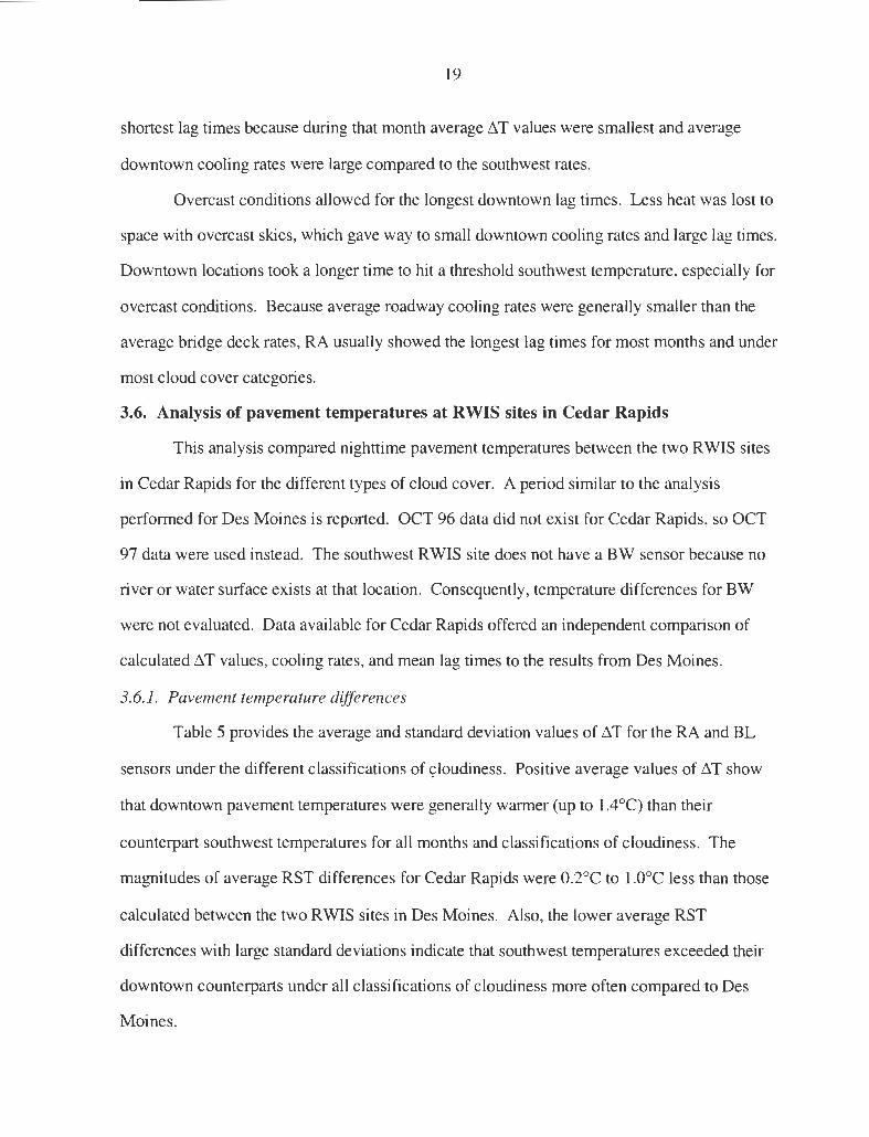
3.6. Analysis of pavement temperatures at RWIS sites in Cedar Rapids
This analysis compared nighttime pavement temperatures between the two RWIS sites
in Cedar Rapids for the different types of cloud cover. A period similar to the analysis
performed for Des Moines is reported. OCT 96 data did not exist for Cedar Rapids, so OCT
97 data were used instead. The southwest RWIS site does not have a BW sensor because no
river or water surface exists at that location. Consequently, temperature differences for BW
were not evaluated. Data available for Cedar Rapids offered an independent comparison of
calculated ~T values, cooling rates, and mean lag times to the results from Des Moines.
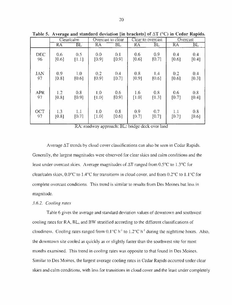
3.6.J. Pavement temperature differences
Table 5 provides the average and standard deviation values of ~T for the RA and BL
sensors under the different classifications of c;loudiness. Positive average values of ~T show
that downtown pavement temperatures were generally warmer (up to l.4°C) than their
counterpart southwest temperatures for all months and classifications of cloudiness. The
magnitudes of average RST differences for Cedar Rapids were 0.2°C to l .0°C less than those
calculated between the two RWIS sites in Des Moines. Also, the lower average RST
differences with large standard deviations indicate that southwest temperatures exceeded their
downtown counterparts under all classifications of cloudiness more often compared to Des
Moines.
20
Table 5. Average and standard deviation [in brackets] of fl T (°C) in Cedar Rapids. Clear/calm Overcast to clear Clear to overcast Overcast
RA BL RA BL RA BL RA BL
DEC 0.6 0.5 0.0 0.1 0.6 0.9 0.4 0.4 96 [0.6] [ 1.1] [0.9] [0.9] [0.6] [0.7] [0.6] [0.4]
JAN 0.9 1.0 0.2 0.4 0.8 1.4 0.2 0.4 97 [0.8] [0.6] [0.9] [0.7] [0.9] [0.6] [0.6] [0.3]
APR 1.2 0.8 1.0 0.6 1.6 0.8 0.6 0.8 97 [0.8] [0.9] [1.0] [0.9] [1.0] [1.3] [0.7] [0.4]
OCT 1.3 1.1 1.0 0.8 0.9 0.7 1.1 0.8 97 [0.8] [0.7] [1.0] [0.6] [0.7] [0.7] [0.7] [0.6]
RA: roadway approach; BL: bndge deck over land
Average llT trends by cloud cover classifications can also be seen in Cedar Rapids.
Generally, the largest magnitudes were observed for clear skies and calm conditions and the
least under overcast skies. Average magnitudes of llT ranged from 0.5°C to l.3°C for
clear/calm skies, 0.0°C to 1.4 °C for transitions in cloud cover, and from 0.2°C to 1.1°C for
complete overcast conditions. This trend is similar to results from Des Moines but less in
magnitude.
3.6.2. Cooling rates
Table 6 gives the average and standard deviation values of downtown and southwest
cooling rates for RA, BL, and BW stratified according to the different classifications of
cloudiness. Cooling rates ranged from 0.1°C h-1 to l .2°C h-1 during the nighttime hours. Also,
the downtown site cooled as quickly as or slightly faster than the southwest site for most
months examined. This trend in cooling rates was opposite to that found in Des Moines.
Similar to Des Moines, the largest average cooling rates in Cedar Rapids occurred under clear
skies and calm conditions, with less for transitions in cloud cover and the least under completely

Table 6. Average and standard deviation [in brackets] values of cooling rates (°C h"1) for Cedar Rapids. -
Clear/calm Overcast to clear Clear to overcast overcast RA BL BW RA BL BW RA BL BW RA BL BW
SW: 0.3 0.4 0.5 0.6 0.2 0.3 0.1 0.1 DEC 10.51 [0.61 10.41 10.51 10.61 10.51 10.31 10.31 96
D: 0.4 0.4 0.4 0.6 0.6 0.6 0.2 0.3 0.3 0.1 0.1 0.1 10.41 10.41 10.51 10.51 10.61 10.61 10.61 10.41 [0.61 10.41 10.41 10.4J
SW: 0.4 0.6 0.2 0.3 0.3 0.3 0.1 0.1 JAN 10.41 10.61 10.51 L0.61 [0.61 10.61 10.61 10.51 97
D: 0.5 0.6 0.6 0.3 0.3 0.3 0.3 0.3 0.4 0.1 0.1 0.1 10.51 [0.61 10.51 10.61 10.7J 10.71 10.61 10.61 10.61 10.51 10.51 10.51
SW: 1.0 1.1 0.8 0.8 I. I 1.1 0.2 0.3 APR 11.31 11.31 10.91 11.01 [ 1.4J Ll.31 10.81 10.81 N -97
D: l. l 0.9 0.9 0.9 0.8 0.7 1.2 1.0 1.0 0.2 0.2 0.2 11.41 11.21 11.11 [1.01 11.01 10.91 11.7) 11.21 Ll.21 10.71 10.61 10.61
SW: 1.0 I. I 0.6 0.7 0.9 0.9 0.4 0.4 OCT 11.11 11.01 10.81 10.81 11.2] 11.11 10.7] 10.71
97 D: 1.1 1.0 0.9 0.7 0.6 0.6 I. I 0.9 0.9 0.5 0.4 0.4
11.31 11.01 10.91 [0.91 10.81 10.71 11.21 10.91 10.91 10.21 10.81 10.81 RA: roadway approach; BL: bridge deck over land; BW: bridge deck over water; SW: southwest site; D: downtown

22
overcast conditions.
Pavement temperatures either rose or didn ' t cool rapidly after 0430 LST under the
different classifications of cloudiness. Early morning RST warming may have led to the large
standard deviation values for the downtown and southwest site cooling rates. This warming was
frequently observed, usually, an hour or two before sunrise. This trend was similar to that
revealed in the Des Moines analysis. For Cedar Rapids in JAN 97, four out of five cases
showed this warming trend under clear skies and calm conditions, eight out of ten for
transitioning sky conditions and all three cases of completely overcast conditions. In total for
JAN 97, 15 of 18 possible cases revealed that RSTs began to increase about two hours prior to
sunrise. Other months showed similar results.
The data from APR 97 and OCT 97 revealed the largest average downtown and
southwest site cooling rates under all classifications of cloudiness. For the winter months, the
smallest average rates existed for all types of cloudiness. In general, results showed that the
downtown cooling rates equaled or slightly exceeded their counterpart southwest rates up to
0.1 °C h-1 under most cloud cover categories and most months. Also both roadway and bridge
deck cooling rates were similar. These trends were opposite of the results from Des Moines.
3.6.3. Mean downtown lag times
Mean downtown lag times were stratified according to the cloud cover categories
(Table 7). Downtown lag times ranged from 0.0 h to 4.7 h. These lag times were considerably
less than those found from the analysis performed for Des Moines. DEC 96 and JAN 97 had
the largest mean downtown lag times under most classifications of cloudiness. Similar to the
results from the analysis for Des Moines, overcast skies produced the largest lag times in Cedar
Rapids. Generally, the largest mean downtown lag times existed for the RA for most months
and under most of the cloud cover categories. It took the downtown roadway RST a longer
time to reach its counterpart rural RST than it did for the downtown BL RST to reach its
southwest bridge deck temperature. In general, this suggests that the subsurface heat flux at the

23
T bl 7 M a e . ean d t own own a~ f 1mes (h). C d R "d ID e ar ap1 s. Clear/calm Overcast to clear Clear to overcast Overcast
RA BL RA BL RA BL RA BL
DEC 1.5 1.3 0.0 0.2 3.0 3.0 4.0 4.0 96
JAN 1.8 1.7 0.7 1.3 2.7 4.7 2.0 4.0 97
APR 1.1 0.7 1.1 0.8 1.3 0.8 3.0 4.0 97
OCT 1.2 1.1 1.4 1.3 0.8 0.8 2.2 2.0 97
RA: roadway approach; BL: bndge deck over land
downtown RA location allowed for the lower average cooling rates and the longest lag times.
3.7. Summary
The pavement temperature analysis concentrated on how the presence/absence, or
change in cloud cover affected nocturnal pavement cooling patterns at RWIS sites
located in Des Moines and Cedar Rapids. Temperature differences, cooling rates, and mean
downtown lag times were computed for the roadways and bridge decks under different
classifications of cloud cover. The analysis showed that downtown pavement temperatures near
both Des Moines and Cedar Rapids are 2°C to 4°C higher than rural pavement temperatures
under a clear sky but only 1°C to 2°C higher under cloudy conditions or when cloud cover is
changing.
Results from Cedar Rapids were compared to the results from Des Moines. The
population of Des Moines is approximately 200,000 and Cedar Rapids is around 100,000.
Because the surface heat island in Des Moines was slightly larger than the one in Cedar Rapids
(by 0.2°C to l .0°C) and noting the population estimates, it appears that the urban effect is larger
as cities get larger (Oke, 1982; Katsoulis and Theoharates, 1985). Consequently, RST trends
for one city do not necessarily apply to another city.
24
RST cooling trends varied over time. The greatest pavement cooling was observed when
relatively warm daytime temperatures were followed by rapid cooling at night. This trend was
most common in the early (October) and late (April) months. Also, the roadways had different
cooling characteristics compared to the bridge decks. In general, the bridge deck cooled faster
than its counterpart roadway by 0.2°C h·' in Des Moines. However in Cedar Rapids little
difference in cooling rate trends between the roadways and bridge decks was observed.
It is important to note that the results from the pavement temperature analysis are
preliminary since they covered only a few months. Winter, fall, and spring months from other
years may give patterns that depart from the limited period studied here.

25
CHAPTER 4. PAVEMENT FROST ANALYSIS ON IOWA BRIDGE DECKS
4.1. Introduction
Frost frequently forms on pavement surfaces in Iowa during the cold season (October
April), particularly in the early morning under conditions of radiational cooling or warm
advection. Frost accumulations may lead to hazardous conditions for motorists unless
pavement surfaces are treated by chemical solutions. However, treating bridge decks with salt
solutions every time the pavement temperature drops to the freezing point or below is not
practical. For example, tax money pays for the salt used to suppress frost as well as the
maintenance needed on roads damaged by chemical solutions. Also, owners of vehicles pay
millions of dollars per year to fight automobile corrosion due to salt deposition on metal
surfaces (Shao and Lister, 1996). In addition, salt pollutes the local environment by running off
into the adjacent water sources and soil (Shao and Lister, 1996).
The Iowa Department of Transportation (IaDOT) chemically treats roadways and
bridges for frost based on site-specific weather forecasts and real-time Roadway Weather
Information System (RWIS) data. Current RWIS pavement temperatures alert IaDOT
management personnel to freezing conditions at 51 locations across Iowa. Accurate frost
predictions allow the IaDOT to maintain practical frost suppression programs, such as anti
icing and deicing procedures, and minimize negative environmental impacts.
In this study a simple numerical model is developed to predict the depth of frost
accumulation on bridge decks. The model uses current RWIS data and forecasts of dew-point
temperature, air temperature, surface temperature, and wind speed to calculate frost accumulation
on bridge decks in Iowa. The model was tested and evaluated by comparing model-generated
maximum frost depth with daily frost observations by IaDOT maintenance personnel. Curves
of relative operating characteristics were used to evaluate the skill of the modeling procedure. A
linear logistic regression technique was developed to determine the probability that a
maintenance worker will observe frost at the predicted frost depth.

26
4.2. Data
4.2.l. RWJS data
Sensor data from five automated RWIS sites were extracted from the IaDOT data
archives. Bridge deck pavement surface temperatures, 5-m wind speeds, 2-m air temperatures
and dew point temperatures from RWIS sites in Spencer, Mason City, Waterloo, southwest Des
Moines, and Ames, Iowa for 21 cold-season months (1995-1998) were used as model input.
Each automated RWIS site has four to five surface sensors strategically embedded in the bridge
decks. At each RWIS site, the bridge deck sensor that recorded pavement surface temperatures
with the least missing data was used in the model prediction procedure.
4.2.2. Pavement frost observations
During the cold season, maintenance personnel record daily observations of the
presence or absence of frost as viewed from inside a vehicle while making surveys of bridges.
The daily surveys usually are taken between the hours of 0500 LST and 0700 LST. The frost
observations are recorded on official winter maintenance sheets and then archived for litigation
or research purposes. Four hundred sixty two frost observations for which corresponding
RWIS data were available were used in the frost analysis for model verification.
4.2.3. Potential errors
No study is exempt from error in the collected data. The first potential error arises with
the location of the RWIS atmospheric tower relative to the pavement surface. RWIS towers
provide information relating to the pavement surface and snow and ice conditions on the
roadway. However, they may not accurately represent large-scale conditions required for frost
forecasting. The model assumes that the 2-m air temperature, 2-m dew point temperature, and
the 5-m wind speed are measured directly above the pavement surface. In reality, the RWIS
tower and its atmospheric sensors are a few meters removed from the pavement surface.
Secondly, the atmospheric tower is often located at a lower or higher elevation than the adjacent
pavement surface. Thirdly, the low level atmospheric RWIS data may be influenced by the local

27
environment such as grass, soil or snow cover. Finally, the atmospheric and pavement
temperature sensors are accurate to ±0.3 cc over the temperature range of -30 cc to 50 cc.
The wind speed sensing element is accurate to ±2.2 m s·1•
The frost observations may also contain errors. Because the frost observations were
recorded within a large range of time between 0500 LST and 0700 LST, the maintenance
personnel may have missed actual frost deposition. The frost may have melted or sublimed
before 0500 LST or may not have been observable until after 0700 LST. Also, maintenance
personnel may have missed frost accumulations on pavement surfaces since observations are
made from inside a vehicle.
4.3. Procedure
4. 3.1. Linear interpolation
Automated RWIS sensor readings are recorded at irregular time intervals due to IaDOT
internal software programming. The times between readings varied from 5 minutes to 3 hours.
A linear relationship with time for temperature change and wind speed change was assumed
between the readings, and a linear interpolation procedure was created to calculate one minute
values from the original RWIS sensor readings taken at irregular intervals. The original RWIS
data were first converted into one minute values using the linear interpolation procedure before
model frost accumulations were calculated.
4.3.2. Frost fomzation on pavement surfaces
Frost formation on pavement surfaces is influenced by factors as wide-ranging as
atmospheric conditions to the amount of traffic on roadways and bridge decks. Hewson and
Gait (1992) showed that the meteorological conditions most conducive to rapid frost deposition
included clear skies, a shallow layer of moist air in contact with the surface, high water-vapor
content in that layer, a gentle but consistent breeze, recent cold weather, short day-length, and
wind direction. However, the main emphasis in this frost analysis is on surface and near
surface meteorological factors that influence frost deposition. Three conditions must exist for

28
T bl 8 C d.f ~ f t d a e . on 1 10ns or ros ·r epos1 100. 1) The pavement temperature (Tp) must be at or below the melting point. (Tp:::; 273.16 K) 2) The pavement temperature (T p) must be less than the 2-m dew point temperature (T 0 ) and the
2-m air temperature (TA). (TA ~ T 0 > T p) 3) The 2-m dew point temperature (T 0 ) must be near 273 .16 K or well above the pavement
temperature (T p) for a period of time.
frost deposition (Takle, 1990) which are described in Table 8. The first condition ensures that
when the pavement temperature is at or below the melting point, any moisture deposited will be
in the form of frost rather than liquid (dew). The second condition ensures that the moisture
available in that 2-m layer has a downward flux onto the pavement surface. The third condition
suggests that greater differences between the pavement and dew point temperature lead to
substantial amounts of frost deposition. In addition, when the deposition period is long, a
significant amount of frost may accumulate on the pavement surface, possibly sufficient to
cause slippery conditions.
The frost accumulation model (F AM2000) described in Section 4.4 uses the three basic
conditions in Table 8 as well as wind speed to estimate frost formation. Moderate wind speeds
at 5-m provide low-level wind shear to promote water-vapor diffusion toward the surface
through turbulent processes. A linear relationship between the wind speed and frost deposition
is assumed and used in the frost model. Figure 4 illustrates RWIS meteorological and
pavement temperatures (based on the criteria outlined in Table 8) accompanying observed frost
formation on a bridge deck near Mason City, Iowa on January 19, 1997.
4.3.3. Basic assumptions
Several factors can affect frost deposition. Salt solutions applied to the pavement
surface act to inhibit frost formation as long as the solutions remain undiluted. Because the
IaDOT does not record the times when salt is used or the amount of salt applied to pavement
surfaces, this analysis assumes that no residual salt is present on the bridge decks analyzed.
Thus, residual salt is not taken into account in the frost accumulation model. In addition, the
frost model assumes that no snow or liquid water is present on the pavement surface to promote

35 0.1
30
,-... It- 25 '-'
~ ::I
~ Cl) e ~ 20
\ \ \
15
\ \ \
' ' ' " ...... ... // ....... __ / ' '
//
/ /
/ I
I I
I
// / ___ /
/ ...... ...... I
...... , /
/
• Dew point temperature
- - -' - Pavement temperature
---Total frost accumulation
I I
I I
I
0.05
0
-0.05
-0.1
IO -0.15
21 22 23 0 2 3 4 5 6 7 8 9 IO 11
LST (h)
Figure 4. Conditions accompanying frost formation.
,-...
e e '-' c: 0
·~ :; e ::I u u ell ..... Cll 0
<!::
~ E-
N
'°

30
or suppress frost formation. This assumption may lead to the underestimation (snow) or
overestimation (water) of deposited frost on roadways and bridge decks. The frost model also
assumes that no precipitation has fallen immediately before or during frost deposition (which
may underestimate accumulations) or after deposition (which may overestimate frost
accumulation or melt any frost away before the maintenance personnel made their daily
surveys). It is important to note that cases where the criteria for frost deposition (Table 8) were
met and precipitation occurred during the deposition period were eliminated from this study.
Only three cases met these conditions.
4.4. Frost accumulation model
The frost accumulation model (F AM2000) calculates the total depth of frost
accumulated on bridge decks over time. The model uses the basic physics of pavement frost
formation found in Section (4.3 b). Consequently, the model frost accumulation is essentially
controlled by the bridge deck temperature, the moisture content of the air near the surface and
the near surface wind speed.
The governing equation used within the model to represent the net flux of moisture, Ff'
onto the pavement (Rayer, 1987; Barker and Davies, 1990; and Sass, 1992, 1997) is
(l)
where Pct is the density of dry air, w' represents the turbulent vertical velocity, and q/ is the
specific humidity with all variables being under saturated conditions at the surface. Using the
transfer coefficient formulation to parameterize (1),
Fr = PctCEU(q5(a) - q/ g)) (2)
where q5(a) is the specific humidity of air at 2-m and q5(g) is the specific humidity of air at the
pavement surface. The transfer coefficient, CE= 10-3 (see Stull, 1988), is held constant due to
the assumption that the stability of air is fixed. U is the 5-m RWIS wind speed (m s-1) . By use
of Dalton's Law of partial pressures (p = e + Pct) and the ideal gas law, equation (2) becomes
(3)

31
which is similar to that used in Hewson and Gait ( 1992) where e is the actual vapor pressure at
2-m, es(T p) is the saturation vapor pressure of the surface pavement temperature, and TA is the
2-m RWIS air temperature. Rct is the gas constant for dry air with units of J kg- 1 K 1, and Eis
the ratio of molecular weights between water and dry air. All temperatures have units of
Kelvins. The difference in saturation vapor pressures, D, between the atmosphere and the
pavement surface is calculated by use of the Clausius-Clapeyron equation,
D = e5(T0 ){exp[LJRv(T0 -1 -T0 -1)] - exp[LJRv(T0 -1 -Tp-1)]} (4)
where L0 is the latent heat of deposition at the freezing point with units of J kg- 1• Rv is the gas
constant for water vapor with units of J kg- 1 K 1, and e5(T 0) is the saturation vapor pressure at T 0
= 273.16 K with units of Pascals. To allow for weak deposition when conditions are just
saturated (T 0 = T p) a small adjustment to the 2-m RWIS dew point temperature is performed,
T0 = Tr+ 0.1. (5)
The rate of growth in depth of frost as a function of time (in m s- 1) can be expressed as
R(t) = Pr- 1ERct- 1CEUDT /, (6)
after equation (3) is divided by a constant density of frost (Pr= 0.1 g cm-3). The complete
derivation of equation (6) is given in Appendix A. Melting of frost is determined from the
snow melt equation (SME) in NCEP' s Eta model for Tr> 273.16 K, where the melt (SMEj is
SME = (-lOE(Tr - 273.16)(T/F+l)Tr- 1). (7)
SME has units of m s- 1, and E = 1.0513 x 10⁻³ m s- 1 and F = 6.48 x 10⁻³ K 4 are constants in the
melting equation. Equations (6) and (7) are multiplied by 1000 mm m- 1 and 60 s min- 1 to get
rates with final units in mm min- 1• The model allows for a downward net flux of moisture
(deposition) onto the pavement surface (A), an upward net flux of moisture (evaporation or
sublimation) from the pavement surface (B), melting of frost with no deposition of moisture
allowed on the pavement surface (C), and melting as well as evaporation or sublimation of frost
at the same time from the pavement surface (D). The growth rate of frost, R(t), can be
summarized in equations (8).

R(t) =
32
(A)=::::} [if T p ~ 273.16 Kand D > 0 then R(t) > 0]
(B) =::::}[if T p ~ 273.16 Kand D < 0 then R(t) < 0]
(C) =::::}[if T p > 273.16 K where R(t) = SME (8) then R(t) < 0]
(D) =::::}[if T p > 273 .16 Kand D < 0 then R(t) < 0]
(8)
The time interval between the calculations, ~t, is one minute. Finally, total frost depth (TFD) is
the aggregate of incremental increases and decreases in frost depth as long as the sum is not
negative (9),
TFD = L R(t) ~t. (9)
The source code for FAM2000 is given in Appendix B.
4.5. Model results
RWIS data gathered from the five RWIS sites were used as input for several
frost model runs. For the 462 frost observations, the model produced 88 cases of positive frost
accumulations (Appendix C), ranging from a low of 10·5 mm to the largest value of
approximately 0.07 mm. For those cases, highway maintenance personnel observed frost on
pavement surfaces 42 times (hits) and did not observe frost 46 times (false alarms). In addition ,
6 events occurred where no frost was calculated by the model, but maintenance personnel
observed frost on pavement surfaces (misses). Finally, the remaining 368 observations (correct
negative prediction), in which the model produced no frost accumulations, were associated with
the absence of frost observed by IaDOT winter maintenance personnel.
A thorough review was completed to find the reason behind the 6 missed events. All the
missed events occurred between December 1995 and January 1996 in Waterloo. RWIS data in
Waterloo and surrounding locations showed that the 2-m dew point temperature and the 2-m air
temperature was less than the pavement temperature generally under overcast conditions. In
addition, the data from the Waterloo RWIS site correlated well with adjacent site data.
Consequently, the model did not produce any frost accumulation. The review indicated that

33
bridge deck frost would not have been caused from radiation cooling effects or warm air
advection processes. Other than the possibility of human error, recent snows and overnight re-
freezing conditions may have been the cause of the frost observations.
From this we conclude there may be a systematic discrepancy between modeled and
observed frost for the Waterloo site for this 2-month period. Resolution of this discrepancy
could very well increase accuracy of the model beyond the level discussed in the following
sections.
4.6. Binary contingency table methodology, results and discussion
4.6.1. Methodology
A binary contingency table approach is used to compare the results of forecasted frost
accumulations to the human frost observations (Table 9). The model frost predictions were
Table 9. Binary contingency table. Human Observations
y N A B
y Hits False Alarms
Forecast c D Correct
N Negative Misses Prediction
used to calculate probability of detection (also commonly known as "hit rate") and a false
alarm rate. Previous studies have agreed on the definition of probability of detection (POD) or
hit rate (H),
H=N(A+C). (10)
However, there is disagreement on the equation used to calculate the false alarm rate (FAR).
For example, the form of the FAR equation ( 11) found in Wilks ( 1995) is
FARl = B/(A + B), (11)
while another form of the FAR equation (12) is given by Mason (1982), Swets (1988),
FAR2 = B/(B + D) (12)

34
and Tak.le (1990).
Marzban (1998) used a binary contingency table approach to define a "rare-event
situation" while applying the equation from Wilks (1995). A rare-event situation is determined
when D >> B, the number of misses is on the same order of magnitude as the number of hits
(C - A), and N0 = (B + D) >> N 1 =(A+ C). It is important to note that the value of D would
increase significantly while the other factors (A, B, and C) would probably remain unaffected if
warm season frost calculations were added into the contingency. Also, C will approach or equal
the order of magnitude of A as more cold season events are analyzed. Using the cold season
results from Table 9 and the technique from Marzban, the formation of frost on bridges is
classified as a rare-event situation. Therefore I choose equation (11) as being most applicable
to frost analysis, although both forms are calculated for comparison.
4.6.2. Results
The values of the hit rate, H = 0.875, and the false alarm rates, FARl = 0.523 and FAR2
= 0.111, suggest that the model did detect frost events well based on the information outlined in
Table 9.
The frequency distribution of (the log of) frost depths (Figure 5) reveals a bimodal
pattern with most likely depths being between 0.002 mm and 0.017 mm. Both curves were
tested for normality. The curve that represents the predicted model depths where observed frost
(hits) was determined to be non-normally distributed with a skewness toward larger calculated
accumulations. However, the positive frost accumulations in which IaDOT personnel did not
observe frost (false alarms) were approximately normally distributed. The Wilcoxen Rank Sum
hypothesis test was used to determine if the two separate curves have significantly different
population means even if the curves are not necessarily normally distributed. The null
hypothesis (that the two curves have the same population mean) failed, thus, indicating that the
two population means are significantly different confirming that the frost model FAM2000 is
capable, in a statistically significant sense, of distinguishing frost occurrences from the non-
14~~~~~~~~~~~~~~~~~~~~~~~~~~~
r-
12
10
[/)
I I I Q) rm -u c: ~ 8 ::s
i J .0 rl n I I I I E ::s z
4
J l I I I J _1, 0 +---~-r-'-.....___, ............ .__ '- .._ .__ .........
2 3 4 5 6 7 8 9 10
Negative natural log of frost depth (mm)
Figure 5. Frequency distribution of (the log of) frost depths.
I I D Frost observed (Hits)
•Frost not observed (False alarms)
11 12 13
w VI

36
occurrences.
A minimum (greater than zero) frost accumulation is required to be visible by humans.
By moving the threshold value for observable frost from 0 mm (as used in Table 9) to higher
values, the false alarm rate improves as the hit rate degrades. Regardless of the threshold used,
FARl gives higher false alarm rates than FAR2. Table 10 and Table 11 show the computed
rates for the various thresholds. Appendix D gives the contingency table adjustments for the
various threshold frost depths. In Figure 6 are plotted the hit and false alarm rates for bridges
for various values of model threshold frost depths using both forms of the false alarm rate
equations.
The general trend in Figure 6 is for both hit and false alarm rates to decrease as the
threshold depth increases. The best choice of threshold was defined to be the value that best
discriminates between frost and no frost, i.e. the greatest difference between hit rate and false
alarm rate (Llli. =hit rate - false alarm rate). When computing false alarm rates using FARl, the
best result, Llli. = 0.389, occurred with the threshold depth of 0.002 mm. However when using
FAR2, the best result, Llli. = 0.769, occurred with a much lower threshold of 10·5 mm.
4.6.3. Discussion
When no frost was observed by maintenance personnel but TFD > 0 (false alarms), the
predicted depths tended to be on the lower end of the range of calculated accumulations and
cases where frost was observed, and TFD > 0 (hits) mostly occurred for the higher end of the
range of accumulations. This suggests that the low values of frost accumulation may
correspond to events for which frost may be accumulating but not to a depth observable by
IaDOT procedures.
The stated goal is to correctly forecast all real frost events and limit the number of false
alarm events. Additional work, not presented in this study, has shown that an adjustment to the
2-m dew point in the original frost model based on meteorological principles reduced false
alarms while correct forecasts were unaffected (Nichols, 1999). However, further testing is

0.9
0.8
0.7 VJ v ..... ~ § 0.6 ~
--; v 0.5 VJ
~ -g 0.4 ~ .....
::2 0.3
0.2
0.1
0
' ' '
---Hit rate
----FARl
---•--·FAR2
', ~ I :j
' '
--- -------------------, ---------.............. --.................... ____ __
~~---------·---------·---------·---------
0 0.002 0.004 0.006 0.008 0.01
Threshold frost depth (mm)
Figure 6. Effect on Hand FAR of various thresholds.
0.012 0.014 0.016 0.018

Table 10. SDT calculations with F ARl. Threshold Hit rate False alarm ~R
depth (H) rate (H-FARI) (mm) (FARI)
0 0.875 0.523 0.352 10-s 0.875 0.512 0.363 10-4 0.813 0.500 0.313
0.000335 0.771 0.486 0.285 10-3 0.729 0.426 0.303
0.002 0.729 0.340 0.389 0.007 0.542 0.257 0.285 0.018 0.271 0.133 0.138
AVG
Table 11. SDT calculations with F AR2. Threshold Hit rate False alarm ~R
depth (H) rate (H-FAR2) (mm) (FAR2)
0 0.875 0.111 0.764 10-5 0.875 0.106 0.769 10-4 0.813 0.094 0.719
0.000335 0.771 0.085 0.686 10-3 0.729 0.063 0.667
0.002 0.729 0.043 0.686 0.007 0.542 0.022 0.520 0.018 0.271 0.005 0.266
AVG
Decision criterion Index of accuracy (Xe) (d')
-0.06 1.09 -0.03 1.12 0.00 0.89
0.035 0.78 0.19 0.80 0.41 1.02 0.65 0.76 1.11 0.50 0.29 0.87
Decision criterion Index of accuracy (Xe) (d')
l.22 2.37 1.25 2.40 l.32 2.21 l.37 2.11 1.53 2.14 1.72 2.14 2.01 2.12 2.57 1.96 1.62 2.18
Criterion placement ((3)
0.48 0.52 0.67 0.76 0.85 0.90 1.23 1.54 0.87
Criterion placement ((3)
1.08 1.13 l.61 1.94 2.68 4.02 7.49 22.56 5.31
VJ 00

39
needed to conclusively evaluate this preliminary model improvement. Also other adjustments to
IaDOT winter procedures could act to improve the quality and accuracy of model verification,
such as, if IaDOT personnel recorded the exact time of frost observance, recorded the amount
of chemical solution used to suppress frost accumulation, and increased the time period in the
morning they look for frost deposition.
4.7. Forecast accuracy and decision criterion
4. 7.1. Signal detection theory
Signal detection theory (SDT), outlined in Mason (1982a), is a technique used to
separate forecast accuracy from the decision criterion. Essentially, SDT is an extension of
probabilistic forecasting using binary contingency table methodology. The SDT technique has
been applied to forecasts of a variety of weather variables (Mason, l 982b; McCoy, 1986; Takle,
1990 and Buizza et al., 1999). SDT is used in this frost analysis in which the probabilistic
forecast is a set of contingency tables where the hit and false alarm rates were computed based
on different threshold frost depths.
The SDT technique, described by Green and Swets (1974) and Swets (1973, 1986,
1988), allows for computations of indices d' and~. The basic SDT index of accuracy, d', is
defined as the number of standard deviations separating the means of the (assumed normal)
distributions of decision criterion preceding occurrence (hits) and preceding non-occurrence
(false alarms). Thus, if the probabilities of the hit rate and false alarm rate are equal, d' = 0
which indicates no skill. Higher values of d' indicate greater skill. The criterion placement, ~' is
the likelihood ratio that measures the occurrence against the non-occurrence. A high criterion
placement value(~> 1) ensures a low false alarm rate at the expense of a lower hit rate. A low
criterion placement value(~< 1) suggests a bias toward maintaining a high hit rate at the
expense of a higher false alarm rate, and a value of~ = l shows no bias towards the hit or false
alarm rate. Table 12 defines the terms used to compute SDT values.

40
Table 12. Signal detection theory (SDT) definitions.
decision criterion= xe = p-i (1 - F)
index of accuracy= d' = xe - p·1 (1 - H)
criterion placement=~= exp { - 0.5 [d' (d' - 2xe)]}
p·1 =inverse of normal probability distribution function .
4. 7.2. Relative operating characteristic curves
By taking bridge values from Table 10 and 11 , a set of point estimates can be plotted on
a hit rate/false alarm rate graph. These points define a SDT curve called the relative operating
characteristic (ROC) generated from normal distributions (Mason, l 982a; Swets, 1986). The
range of threshold frost depths observed in our study does not span the entire range of hit and
false alarm rates, but the limit cases must tend toward the points (0,0) and (1 ,1). Figure 7 is a
curve of hit rates and false alarm rates (FAR!) for various frost depths. A comparable plot for
the same range of threshold frost depths but using the other form of the false alarm rate
equation (F AR2) is shown in Figure 8.
The goal of using the ROC curves is to find an "optimum" combination of hits and
false alarms and to quantify the impact of lowering FAR or raising H. Results from Figure 7
and Table 10 show that the optimum combination of high accuracy and large criterion
placement is for the threshold frost depth at 0.002 mm where d' = 1.02 and ~ = 0.90. The best
results for FAR2 (Figure 8 and Table 11) are found for the same threshold frost depth (0.002
mm) where d' = 2.14 and ~ = 4.02, which indicates a higher accuracy with a strong bias toward
minimizing false alarms.
4. 7.3. Area under the ROC curves
Following Swets (1988), another measure of accuracy is defined as the area (A) under
the ROC curve. If A= 1, the probabilistic forecast system is considered perfect, with accuracy
decreasing with decreasing A. A= 0.5 gives a useless forecast system. More specifically a

41
-. 0 .9
0.8
t-0 .7 -
I
u.. 0 C' .6
>-1-_J -
l'CD < rn 0.4 0 a:: n..
0 . 1 0.2 0.3 0.4 0 .5 0 .6 0.7 0.8 0 . 9 1.1
PROBABILITY OF FALSE ALARM
Figure 7. The set of black dots defines the ROC curve using point estimates of H and FARl for the various threshold frost depths.

i-~
I
lL 0
>-~
_J
CD <l co 0 0:: a_
0 .8
0 .7
0.6 .
0 .!>
0.4
42
O.l 0.2 0.3 0.4 0.5 0 .6 0.7 o.e 0.9
PROBABILJTY OF FALSE ALARM Figure 8. The set of black dots defines the ROC curve using point estimates of H and
FAR2 for the various threshold frost depths.
l

43
a perfect forecast system has a 100% hit rate and 0% false alarm rate (A= 1), while a useless
system has a ROC curve that coincides with the diagonal (d' = 0) on the ROC curve and an area
under the curve A= 0.50. Swets suggests that A values less than 0.70 lead to insufficient
accuracy in the forecast system to provide much practical value, and values between 0.70 and
0.90 define sufficient accuracy in the system. However, a few texts warn of the use of arbitrary
threshold values to define system accuracy (Buizza et al., 2000; Juras, 2000; Wilson, 2000)
using the area under the ROC curve. For example, Juras (2000) argues that the limit value for
A should vary and depend on the variability of climatological frequencies of an event within a
homogeneous region.
Integration of the area under the ROC curve given in Figure 7 for bridges yields a value
A= 0.71 and from Figure 8 A= 0.91. Thus, using the qualitative threshold criterion range
(0.70-0.90) from Swets, the frost model (FAM2000) has potential practical value. Even
though the A value of forecasts made with the frost model may be reduced by the uncertainty in
the input data, F AM2000 has the potential to be skillful. Also, these results indicate that
FAM2000 has slightly higher accuracy than the expert system used in Takle (1990).
4.8. Logistic regression model
Logistic regression analysis is a well known statistical procedure commonly used in
many scientific fields of study (Agresti , 1984; Freeman, 1987; Hosmer and Lemenshow, 1989).
Here it is used to investigate the relationship between the binary response (frost observations)
and the explanatory response (model frost depths) variables. Cox and Snell (1989) give a
thorough discussion of binary response model methodology.
A simple linear logistic regression model (13) was used to describe the probability of a
predicted frost depth being observed by IaDOT personnel given a particular calculation of frost
depth by the model:
log (p/(l - p)) =a+ ~x (13)
Let x be the predicted frost depth (TFD in Eq. 10), and p be the probability of observed frost ,

44
leaving (1 - p) as the response probability frost was not observed. By use of maximum
likelihood analysis (Aitchison and Silvey, 1957 and Ashord, 1959), the intercept estimate, a ,
was calculated to be -3.0575, and the slope estimate , ~. was 296.9. Solving for p gives
(14)
If forecast values of air temperature, dew point temperature, pavement temperature, and wind
speed are used to drive the frost accumulation model to provide x ( = TFD) then (14) gives the
probability that an IaDOT employee will see frost under the predicted conditions.
Figure 9 shows the logistic regression curve for the probability of observing frost (p)
for various values of predicted frost depths (x = TFD). The general trend in Figure 9 is for p to
increase as the depth increases. Results in Figure 9 show that when p = 1 (~ 0.1), x 2:: -0.03
mm (~ 0.003 mm) and show that the minimum threshold frost depth to be observed by a human
within a maintenance vehicle is approximately 0.01 mm (p = 0.50), which is at the upper end of
the range (0.002 -0.01 mm) of observable depths suggested by Hewson and Gait (1992).
Therefore frost depths less than 0.01 mm are less likely to be observed by IaDOT maintenance
personnel than those exceeding 0.01 mm. Also, under extreme frost deposition , total frost
depths equal to or greater than 0.03 mm (p = 1) are more likely to be observed by laDOT
maintenance personnel.
4.9. Summary
A model (FAM2000) based on simple concepts of moisture flux to the surface has been
developed based on current and forecasted RWIS air temperatures, dew point temperatures,
pavement surface temperatures, and wind speed. The model uses the RWIS data to calculate
expected amounts of accumulated frost (TFD) on bridges. Bridge deck frost was shown to
arguably be a rare-event situation; therefore, forecast skill of the model was evaluated using the
false alarm rate (12) appropriate for rare events. Results from the SDT and ROC analyses
suggest that the prediction of frost on bridge decks by use of the model has sufficient accuracy
to be used as an operational tool ; however, uncertainty of input information (i.e. forecast RWIS

0.8
'2. 0.6 '-"
.f' -:..0 <:IS
..0 e 0... 0.4
0.2
- Linear logistic regression curve
0 1--~~-.--~~--.-~~~~~---.-~~~..--~~-.--~~-,.-~~---..,.-~~---,.~~----i
0 0.003 0.006 0.009 0.012 0.015 0.018 0.021 0.024 0.027 0.03
Predicted frost depth (mm)
Figure 9. The probability (p) that IaDOT personnel will see frost for a predicted frost depth.
~

46
values) will correspondingly degrade the prediction of frost accumulation.
A key parameter determined was the threshold accumulated frost depth calculated by the
model that corresponds to the minimum observable frost seen by IaDOT maintenance
personnel from inside a moving vehicle while making surveys of bridges. A logistical
regression technique was used to determine the probability (p) that a maintenance worker will
observe frost for a given calculated frost depth (TFD). Results indicated that a threshold depth
of around 0.01 mm seems to be the minimal likely amount of frost accumulated on a bridge
deck that is observable under IaDOT procedures.
Finally, some assumptions used in the simple model (e.g., use of neutral drag
coefficient) and its application to an elevated surface (e.g., elevated bridge deck as opposed to a
flat surface of infinite horizontal extent at the ground) might introduce biases into the model.
Limitations of observations (e.g., frost occurring after observer has completed his/her
observation, frost not forming due to residual frost-suppressing chemical) also may reduce
accuracy of the model. A systematic comparison of model calculations with observations would
allow evaluation of model accuracy and suggest ways of tuning for improvement.

47
CHAPTER 5. CONCLUSIONS
This study examined the use of RWIS data in the fight against nocturnal slippery road
conditions during the cold season for site-specific locations in the state of Iowa. The study
centered around the development of a few forecast procedures based on simple physical
concepts about the prediction of pavement temperature cooling and moisture deposition in the
form of frost on bridge decks.
The pavement temperature analysis (Chapter 3) concentrated on the meteorological
effects of RST cooling due to cloud cover and seasonal effects. Urban and rural RST cooling
trends offer roadway maintenance personnel guidance for treating roadways and bridges for
frost, snow, and ice conditions as well as supplementing pavement temperature forecasts. For
example, maintenance personnel can compare the calculated cooling rate trends for bridges and
roadways to pavement temperature forecasts provided to them by their private weather
forecasting source. This comparison could lead to a refinement on the timing of onset of
freezing conditions at specific RWIS locations. In general, the calculated cooling rates and
mean urban Jag times can be used as a tool in combination with other forecast products to
determine expected pavement cooling for Des Moines and Cedar Rapids. Cooling trends were
not always the same, so it is important to note that pavement temperature cooling trends for one
city can not necessarily be applied to another city.
The frost analysis (Chapter 4) focused on the prediction of frost on bridge decks based
on RWIS temperature and wind speed data from five Iowa sites. When maintenance personnel
are faced with the threat of nocturnal frost formation, they factor non-meteorological as well as
meteorological information into their prevention plans. When considering all information
available, IaDOT management can use the SDT procedure to determine the optimum
combination of hit rate and false alarm rate based on the established threshold frost depths. For
example, when they receive a forecast frost accumulation, management can use the SDT
procedure to evaluate the forecast accuracy in combination with available non-meteorological

48
information (i.e. residual salt residue on pavement surfaces, traffic volume, or environmental
issues). In addition, management can compare the results of logistic regression probability of a
forecasted maximum frost depth to internal frost prevention standards within the IaDOT.
This study offers forecast procedures to aid in the prediction of slippery road conditions
across Iowa during the cold season. The procedures developed concerning pavement
temperature cooling and frost formation give management personnel tools to help manage and
forecasters tools to help forecast frost events.

49
APPENDIX A. DERIVATION OF FROST ACCUMULATION MODEL
Net flux of moisture onto the pavement:
Ff =Pct (w' q; )s Pct=> density of dry air w' => turbulent vertical velocity q' => specific humidity ( \ => indicates saturation at surface
Parameterization by use of transfer coefficient formulation: Ff=> PctCEU (qs(a) - qs(g)) CE => transfer coefficient qs(a) =>specific humidity of air at 2-m qs(g) =>specific humidity of air at pavement surface U => 5-m wind speed
Hint: Units of Ff are (mass)(area x timer1 => gcm-2s- 1
Use Dalton law of partial pressures and ideal gas law: E = 0.622 p => atmospheric surf ace pressure
e =es (T0 )exp{ LctRv-t ((T0 - 1) - (TP.- 1))}
e => saturation vapor pressure at 2-m qs(a) = Eep- 1
=> Ep-1es (T0 )exp{ LctRv-l ((T0 - 1) - (Tct- 1))}
es (TP) =es (T0 )exp{ LctRv-t ((T0 - 1) - (TP.-1))} es (TP) =>saturation vapor pressure at the pavement surface, TP qs(g) = Ees(TP)p-1
=> Ep-1es (T0 )exp{ LctRv-I ((T0 - 1) - (TP- 1))}
T0 =>freeze point= 273.16 K es (T 0) => saturation vapor pressure at freeze point = 6.108 mb Lct =>latent heat of deposition Rv => the specific gas constant for water vapor
Let: Ff = CEU ([Ep-1es (T0 )exp{ LctRv- I ((T0 - 1) - (T/))}]
- [Ep-1es (T0 )exp{ LctRv-l ((T0 -1) - (T/))}])
Ff = CEUEp- 1es (T0 ) ([exp{ LctRv-l ((T0 - 1) - (Tct-1))}] - [exp{ LctRv-l ((T0 - 1) - (TP- 1))} ])Ta-l
Substitution: let D =es (T0 )([exp{ LdRv-l ((T0 - 1) - (T/))}] - [exp{ LctRv-l ((T0 - 1) - (TP- 1))}])
To get growth in depth of frost with time, divide Fr (gcm-2s- 1) by the density of frost.

Assume density of frost: Pr:::::} 0.1 x density of ice, pi= 1.0 (gcm-3)
Pr:::::} 0.1 x pi = 0.1 (gcm-3)
Rate of growth of frost with time: R(t):::::} Ff Pr-1 = Pr-1CEU£Rd-1DTa-1
Simplify: R(t) = Pr-1£Rct-1CEUDT.-1
50
R(t) is the governing equation to determine the frost accumulation rate.
51
APPENDIX B. FROST ACCUMULATION MODEL (FAM2000) SOURCE CODE
FROST ACCUMULATION MODEL (F AM2000)
PROGRAM DISCUSSION
THIS IS A FORTRAN 90 DRIVER PROGRAM. THIS PROGRAM WAS CREA TED AND MAINTAINED BY DAVID KNOLLHOFF. CREATION DATE (AUGUST 2000).
! THIS PROGRAM ACCEPTS DATA WITH A DATE AND TIME STAMP AS WELL AS 2-M AIR TEMPERATURE .. . 2-M DEW POINT TEMPERATURE .. . 5-M WIND SPEED AND PAVEMENT TEMPERATURE. THE PROGRAM QUALITY CONTROLS THE DATA STATING ANY ERRORS FOUND. THEN THE TIME/DATE STAMP IS CONVERTED INTO TOTAL MINUTES USING THE FUNCTION convert_date2min.f90. NEXT THE PROGRAM GOES THROUGH ANOTHER QUALITY CONTROL CHECK TO MAINTAIN CHRONOLOGICAL ORDER OF DATA. IF ERRORS ARE FOUND THE USER WILL BE NOTIFIED. THEN ONE MINUTE VALUES ARE CREATED USING A SUBROUTINE CALLED lin_inter.f90 (LINEAR INTERPOLATION). AFTER THE LINEAR INTERPOLATION PROCESS HAS COMPLETED . .. THE PROGRAMS CALLS ANOTHER SUBROUTINE accumulation5.f90 TO CALCULATE (PREDICT) THE TOTAL DEPTH OF FROST ACCUMULATED FOR A BRIDGE DECK IN IOWA. FINALLY THE MINUTE
! VALUE OF THE DATEfTIME STAMP IS CONVERTED BACK INTO THE ! EQUIVALENT CALENDAR DA TE AND TIME. THE DATA IS PRINTED TO THE ! SCREEN AND/OR A FILE NAMED outputl.
' DEFINITIONS
max dim maxnum yy mm dd hr mtime
! savetime ! ierrcnt ! dt !m ' . . 1
! ict ! nvalues ! aircnt ! dewcnt ! errorcnt ! speedcnt ! pavecnt ! assumecnt ! air ! dew ! speed
= maximum number of lines allowed from calculations =maximum number of lines allowed from input file = 2 digit calendar year from input file = 2 digit calendar month from input file = 2 digit calendar day from input file = 2 digit hour from archive file =the value in total minutes calculated using convert_date2min.f90 function
(minutes) = the stored old mtime = number of errors from the chronological test =the difference in time between consecutive observations (min) = loop counters for final data point = loop counters for initial data = counter for final data point = the number that represents the total number of lines in file =number of errors in air temperature data . = number of errors in dew point temperature data = total number of air in meteorological data =number of errors in wind speed data = number of errors in pavement temperature data = number of errors from meteorological assumptions = air temperature data (F) =dew point temperature data (F) =wind speed data (mph)

52
! pave = pavement temperature data (F) = air temperature difference (F) ' ar
slopeair dw slopedw spd
= slope of air temperature over time (F/min) =dew point temperature difference (F) =slope of dew point temperature difference over time (F/min) =wind speed difference (mph)
slopes peed p slopepave prob
= slope of wind speed over time (F/min) = pavement temperature difference (F/min) = slope of pavement temperature (F/min) =probability of seeing a predicted frost depth (mm)
INITIALIZATION
parameter (maxdim=90000) parameter (maxnum=lOOOO) integer convert_date2min integer yy,mm,dd,hr,min integer yyy ,mmm,ddd,hhh,mmin integer mtime(maxnum),savetime,ierrcnt,dt,newmin(maxdim) integer m,NN,Mf ,ict,aircnt,dewcnt,errorcnt,speedcnt,pavecnt integer assumecnt,I,nvalues real*8 air(maxnum),dew(maxnum),speed(maxnum),pave(maxnum) real* 8 ar,slopeair,dw ,slopedew ,spd,slopespeed,p,slopepave real* 8 TT A(maxdim),TTD(maxdim),WWS(maxdim),TfP(maxdim) real*8 AA,TA,SA,TDD,TD,SD,WSD,WS,SS,PP,TP,SP real*8 smr,R,Rsmr,depth,TFD,prob real *8 cela,Ka,celd,Kd,sped,celp,Kp,b,c,D,D l ,D2 character*80 filein aircnt=O dewcnt=O speedcnt=O pavecnt=O assumecnt=O errorcnt=O savetime=-1 ierrcnt=O ict=O
! FILE OF INTEREST
print *, 'enter the name of your data array' read (5,fmt='(a80)') filein open (unit=200,file=filein,status=' old') open (uni t=20 l ,file=' output l' ,status=' unknown') do i=l,maxnum
read (200,100,end=9) yy,mm,dd,hr,min,air(i),dew(i),speed(i),pave(i) 100 format (2x,i2,lx,i2,lx,i2,3x,i2,lx,i2,4x,fl0.2,lx,fl0.2,lx,fl0.0,lx,fl0.2)
' ! QUALITY CONTROL FOR METEOROLOGICAL ASSUMPTIONS
' if (air(i) .le. - 50.dO .or. air(i) .ge. 120.dO) then print*, yy,mm,dd,hr,min,air(i),'-- does not meet air temp assumption'

53
aircnt=aircnt+ 1 endif
if (dew(i) .le. -50.dO .or. dew(i) .ge. 120.dO) then print *, yy ,mm,dd,hr,rnin,dew(i),' -- does not meet dew temp assumption '
dewcnt=dewcnt+ 1 endif
if (speed(i) .It. 0 .or. speed(i) .ge. 100) then print *, yy,mm,dd,hr,rnin,speed(i),'-- does not meet wind speed assumption '
speedcnt=speedcnt+l endif
if (pave(i) .le. -50.dO .or. pave(i) .ge. 120.dO) then print *, yy,mm,dd,hr,rnin,pave(i),'-- does not meet pavement temp assumption '
pavecnt=pavecnt+ 1 endif
if (dew(i) .gt. (air(i)+l.dO)) then print *, yy,mm,dd,hr,rnin ,dew(i),air(i),'-- does not meet physical assumption '
assumecnt=assumecnt+ 1 endif
errorcnt=aircnt +dewcnt +speedcnt +pa vecnt +assumecnt
CONVERT DATE/TIME STAMP TO MINUTES USING FUNCTION
mtime(i )=convert_date2rnin (yy ,m,dd,hr,rnin)
QUALITY CONTROL FOR CHRONOLOGICAL ORDER
if (mtime(i) .le. savetime) then print *, yy,mm,dd,hr,rnin , '-is out of order' ierrcnt=ierrcnt+ 1
savetime=mtime(i) enddo
endif
print*, 'maxnum exceeds ', maxnum stop 16
9 nvalues=i-1 print *, 'Function date2rninute has been completed successfully! ' if (errorcnt .gt. 0) then
print*, 'Stopping due to', errorcnt, 'error(s) in the meteorological assumptions' stop 17
endif if (ierrcnt .gt. 0) then
print*, 'Stopping due to ' , ierrcnt, 'error(s)' stop 18
endif print *, 'Quality control procedures completed successfully!'

54
CALCULATE INTERVAL DIFFERENCES FOR PARAMETERS
do i=l,nvalues-1 dt=mtime(i+ 1)-mtime(i) ar=air(i+ 1 )-air(i) slopeair=ar/dt dw=dew(i+ 1)-dew(i) slopedew=dw/dt spd=speed(i+ 1 )-speed(i) slopespeed=spd/dt p=pave(i+ 1 )-pave(i) slopepave=p/dt
CREATE ONE MINUTE INTERPOLATION VALUES FOR PARAMETERS
call lin_inter (dt,mtime(i),air(i),slopeair,dew(i),slopedew,speed(i), slopespeed,pave(i), & slopepave,newmin,TTA,TTD,WWS,TTP,ict,maxdim)
enddo
! TAKE CARE OF FINAL DATA POINT
ict=ict+ 1 m=ict TT A(m)=air(nvalues) TTD(m)=dew(nvalues) WWS(m)=speed(nvalues) TTP(m)=pave(nvalues) newmin(m)=mtime(nvalues)
print *, 'Linear interpolation completed successfully! '
! ECHO BACK ALL OF MY MINUTE BY MINUTE DATA TO THE SCREEN
write(201 ,*) 'Date TFD=O.dO do m=l ,ict
Time Depth TFD'
call accumulation (TT A(m),TTD(m),WWS(m),TTP(m),m,smr,R,Rsmr,depth ,TFD, & cela,Ka,celd,Kd,sd,celp,Kp,b,c,D ,D l ,D2)
call convert_min2date (newmin(m),yyy,mmm,ddd,hhh,mmin)
USING LINEAR LOGISTIC REGRESSION TO DETERMINE PROBABILITY (P) OF OBSERVING A PREDICTED FROST DEPTH (TFD)
prob=l .d0/((l .dO+exp(-(-3.0575d0+(296.9dO*TFD)))))
PRINT TO OUTPUT FILE (OUTPUT!)
write(201, 101) yyy ,mmm,ddd,hhh,mmin,depth,TFD,prob 101 format (3i2.2,lx,2i2.2,lx,2fl4.8,lx,f6.4)
enddo print *,'Completed frost accumulation process successfully! ' print *,'You have created one output file . Check out the following file: '

55
print*,' outputl'
CLOSING FILES ... END OF DRIVER PROGRAM
close (unit=200) close (unit=201) stop end
function convert_date2min (yy,mm,dd,hr,min)
! THIS IS A FORTRAN 90 FUNCTION PROGRAM. THE PURPOSE OF THIS ! FUNCTION IS TO TAKE A CALENDAR DATE AND TIME STAMP AND CONVERT
INTO TOTAL MINUTES. THIS FUNCTION TAKES INTO ACCOUNT THE YEAR 2000 CHANGE OVER AND LEAP YEAR ISSUES. A REFERENCE CALENDAR DATE (01101/93) IS USED. THIS FUNCTION HAS DATA BOUNDS FROM 1993 TO 2020. IF YOU NEED TO USE DATA OUTSIDE THESE BOUNDS ... THE FUNCTION NEEDS TO BE ADJUSTED ACCORDINGLY IN A COUPLE OF LOCATIONS WITHIN THIS PROGRAM. THIS FUNCTION QUALITY CONTROLS THE DATA INCOMING AND WHEN AN ERROR IS FOUND .. . THE PROGRAM STOPS AND PRINTS LOCATION OF ERROR. THE CALCULATIONS IN THIS FUNCTION ARE
! ROUTED BACK TO THE DRIVER PROGRAM. THIS PROGRAM WAS CREATED ! BY DAVID KNOLLHOFF (AUGUST 2000).
' ! DEFINITIONS
' ! convert_date2min ! year ! leapyrs ! totdays ! tdinmo ! lymo ! nlymo ! dinmo
' ! INITIALIZATION
implicit none
=total minutes value for the calendar day and 24 hour time period = dummy variable for yy read in = to determine if your year falls in a four year period = calculation of number of days since Jan l 1993 = variable to account for leap year extra day in February =leap year month (total of days possible) =non leap year month (total of days possible) = days in non leap year month
integer convert_date2min integer yy ,mm,dd,hr,min integer year,leapyrs,totdays,tdinmo integer lymo(l2),nlymo(l2),dinmo(l2) data lymo /0,31,60,91 ,121,152,182,213,244,274,305,335/ data nlymo /0,31,59,90,120,151,l81 ,212,243,273,304,334/ data dinmo /31 ,28,31,30,31,30,31,31,30,31 ,30,31/ year=yy
56
QUALITY CONTROL DATA AND CHECK FOR Y2K
if (year .le. 20) year=year+ 100 ! fix up for 2000-2020 if (year .It. 93 .or. year .gt. 120) then print*, yy,mm,dd,hr,min,' -- YEAR is out of range'
stop 10 endif
if (mm .le. 0 .or. mm .gt. 12) then print*, yy,mm,dd,hr,min,' -- MONTH is out ofrange'
stop 11 endif
if (dd .le. 0 .or. mm .gt. 31) then print*, yy,mm,dd,hr,min,' -- DAY is out of range'
stop 12 endif
if(hr.h. 0 .or. hr.gt. 23)then print*, yy,mm,dd,hr,min,' -- HOUR is out ofrange'
stop 13 endif
if (min .le. 0 .or. mm .gt. 12) then print*, yy,mm,dd,hr,min,' -- MINUTES is out ofrange'
stop 14 endif
! CHECK FOR LEAP YEARS
'
leapyrs=(year-93 )/4 totdays=365 * (year-93 )+ leapyrs if (mod(year-92,4) .eq. 0) then
tdinmo=dinmo(mm) if (mm .eq. 2) tdinmo=29 if (dd .le. 0 .or. dd .gt. tdinmo) then
! for 'prior full years' ! with correction for leap years
! we've got leap year
print*, yy,mm,dd,hr,min,' -- DAY is out ofrange' stop 14
endif totdays=totdays+lymo(mm)
else if (dd .le. 0 .or. dd .gt. dinmo(mm)) then
! months prior to mm - leap year ! not a leap year
print*, yy,mm,dd,hr,min,' -DAY is out ofrange' stop 15
totdays=totdays+nlymo(mm) endif
endif ! month prior to mm -- not a leap year
! CALCULATE MINUTES SINCE JANUARY 1, 1993 (01/01/93)
' totdays=totdays+dd-1 convert_date2min=l440*totdays+60*hr+min ! calculated minutes return end

57
subroutine lin_inter (NN,MT,TA,SA,TD,SD,WS,SS,TP,SP,newmin,TTA,TTD,WWS,TTP, & ict,maxdim)
! THIS IS A FORTRAN 90 SUBROUTINE TO CALCULATE THE MINUTE BY ! MINUTE VALUES FOR 2-M AIR TEMPERATURE . .. 2-M DEW POINT ! TEMPERATURE ... 5-M WIND SPEED AND PAVEMENT TEMPERATURE DATA.
THIS SUBROUTINE IS CALLED IN THE DRIVER PROGRAM PORTION. THIS PROGRAM WAS CREATED BY DAVID KNOLLHOFF (AUGUST 2000).
DEFINITIONS
! newmin ! TIA
=interpolated values of time stamp =interpolated values of air temperature
! TTD ! wws ! TIP
= interpolated values of dew point temperature = interpolated values of wind speed
' . . 1
= interpolated values of pavement temperature = loop counter
' ! INITIALIZATION
! NN=dt ! MT=mtime(i) ! TA=air(i) ! SA=slopeair(i) ! TD=dew(i) ! SD=slopedew ! WS=speed(i) ! SS=slopespeed ! TP=pave(i) ! SP=slopepave
implicit none integer i,m,ict,maxdim integer NN,MT,newmin(maxdim) real*8 TA,SA,TD,SD,WS,SS,TP,SP real*8 TTA(maxdim),TTD(maxdim),WWS(maxdim),TTP(maxdim)
! CREATE ONE MINUTE VALUES
do I=l,NN ict=ict+ 1 if (ict .gt. maxdim) then
print*, 'maxdim too small - STOP - maxdim=', maxdim stop 222
endif m=ict TT A(m)=SA *(i-1)+ TA TTD(m)=SD*(i-1 )+TD WWS(m)=SS*(i-l)+WS TTP(m)=SP*(i-1 )+ TP newmin(m)=MT +i-1

enddo return end
58
subroutine accumulation (IA,ID,IS,IP,ii ,smr,R,Rsmr,depth,TFD,cela,Ka,celd,Kd,sped, & celp,Kd,sped,celp,Kp,b,c,D,D l ,D2)
TIDS IS A FORTRAN 90 SUBROUTINE THAT WILL CALCULATE (PREDICT) THE TOT AL DEPTH OF FROST WITH TIME. THE ONE l\11NUTE LINEARLY INTERPOLATED VALUES ARE USED IN THE ACCUMULATION PROCESS. THE RATE OF SNOW MELT IS TAKEN INTO ACCOUNT WHEN PAVEMENT TEMPERA TURES RISE OR REMAIN ABOVE 32 F. MODEL INPUT NEEDS TO BE IN INCREMENTS OF 1 l\11NUTE INTERPOLATED VALUES TO RUN MODEL CALCULATIONS PROPERLY. PRECIT A TI ON IS NOT TAKEN INTO ACCOUNT. EVAPORATION OF FROST IS ALLOWED WITH MELTING . .. BUT DEPOSITION OF MOISTURE IS NOT ALLOWED DURING MELTING PERIODS.
DEFINTIONS
fOUI
eps ce Rd es To Ld
! Rv To IA ID IS IP con st constl
Dl
D2
D R a celp Kp cela Ka celd Kd sped
'b ! c ! depth !TFD
= density of ice @ 32 F = epsilon-ration of molecular weights of H20/dry air = transfer coefficient =gas constant for dry air = saturation vapor pressure at the freezing point = latent heat of deposition at the freezing point = gas constant for water vapor = freezing point temperature =interpolated air temperatures = interpolated dew point temperatures =interpolated wind speed values = interpolated pavement temperatures =constant given the stability of the air is fixed =ratio of latent heat of deposition at the freezing point over the
specific gas constant for dry air = exponential function of the saturation vapor pressures for the 2-m
dew point temperatures = exponential function of the saturation vapor pressures for 2-m
pavement temperatures = the difference of the two exponential functions = frost deposition/evaporation/sublimation rate = inverse ratio of freezing point temperature =pavement temperature converted from °F into °C =pavement temperature converted from °C into kelvin = 2-m air temperature converted from °F into °C = 2-m air temperature converted from °C into kelvin = 2-m dew point temperature converted from °F into °C = 2-m dew point temperature converted from °C into kelvin = 5-m wind speed values converted from mph in ms-1
=calculation of inverse ratio of dew point temperatures = calculation of inverse ratio of pavement temperatures = frost accumulation depth = total frost accumulation
UNITS
kom-3 0
no units no units Jko-1K 1
0
Pa Jko-1
0
Jko-1K 1 0
K F F Mph F K K
no units
no units
no units mmmin-1
K1 c K c K c K ms- 1
K1 K1 mm mm

!e ! f
= constant for snow melt equation =constant for snow melt equation
59
! smr ! Rsmr
= snow melt rate (taken from ET A model) =calculation of deposition or sublimation
! INTIALIZA TION
! IA=TTA(m) ! ID=TTD(m) ! IS=WWS(m) ! IP=TTP(m) ! ii=m
implicit none real* 8 roui ,eps,ce,Rd,esTo,Ld,R v ,To,e,f,a,const,const 1,D 1,D2,D ,b,c real*8 celp,Kp,cela,Ka,celd,Kd,sped real*8 smr,R,Rsmr,depth,TFD,tdepth real*8 IA,ID,IS,IP integer ii
CHECK WIND SPEED
if (IS .eq. O.dO) then IS=l.dO
CONSTANTS
fOUI = 917 eps = 0.622d0 ce = O.OOldO Rd = 287.0dO EsTo = 610.8d0 Ld = 2834000.0dO Rv = 461.0dO To = 273.16d0
endif
no units no units mms-1
mmmin-1
! e is multiplied by 1000 mm for unit conversions for smr which is originally in units of ms-1•
! This is a more convenient location to do the conversion than down below. ! e = l.0513*0.00000001 *1000.
e = l.0513d-5 f = 0.0000000648d0
CONVERSION OF TEMPERATURES (from °F to °C to kelvin)
cela = (IA-32.d0)/1.8d0 Ka= cela+273.16d0
celd = (ID-32.d0)/1.8d0 Kd = celd+273.16d0
celp = (IP-32.d0)/l.8d0 Kp = celp+273.16d0

60
CONVERSION OF WIND SPEEDS (from mph to ms- 1)
sped= IS*0.44704d0
MODEL: VAPOR PRESSURES, FROST RATES, DEPTH, AND TOTAL DEPTH
if (Kp .eq. Kd) then Kd=Kp+O. lOdO
endif const=(eps/roui)*ce*(esTo/Rd)
const=0.00000 l 443d0 ! constl=Ld/Rv
constl=6147.505423d0 a=l./To
a=0.003660858d0 b=l.dO/Kd c=l.dO/Kp Dl=exp(constl *(a-b)) D2=exp(constl *(a-c)) D=Dl-D2
When multiplied by 60. seconds = 1 minute ! When multiplied by 1000. Mm = 1 meter I
Snow melt rate (smr) is assumed to be in units of (ms-1) then multiplied by 60s/min and by 1000 mm to get final units of mmmin-1 for smr and Rsmr
! Rate of deposition (sublimation) or evaporation of moisture (R) has units of (mmmin-1) for ! each interpolated value. I
if (Kp .gt. 273.16d0 .and. D .It. O.dO) then Scenario #1 melting and evaporation
smr=-( 10.dO*e*((Kp-273.16dO)*(((Kp**4 )*f)+ l .dO))/Kp ))*60.dO R=l000.dO*(const*(sped/Ka)*D*60.dO) Rsmr=(R+(smr)) elseif (Kp .gt. 273.16d0 .and. D .gt. O.dO) then Scenario #2 melting only allowed, Not deposition
smr=-( 10.dO*e*((Kp-273.16dO)*(((Kp**4 )*f)+ l .dO))/Kp ))*60.dO R=l000.d0*(const*(sped/Ka)*D*60.d0) Rsmr=smr elseif (Kp .le. 273.16d0 .and. D .It. O.dO) then Scenario #3 Evaporation/sublimation , no melting allowed smr=O.dO R=l000.dO*(const*(sped/Ka)*D*60.dO) Rsmr=R elseif (Kp .le. 273.16d0 .and. D .gt. O.dO) then Scenario #4 Deposition, no melting allowed smr=O.dO R= 1000.dO*( const*( sped/Ka)*D*60 .dO) Rsmr=R
endif
61
CALCULATION OF FROST ACCUMULATION DEPTHS (depth)
Because l minute interpolated values are used, Rsmr is multiplied by a delta time of l minute to satisfy unit cohesiveness for depth (mm)
if (ii .eq. 1) then depth=O.dO
else depth=(Rsmr* l .dO)
endif
CALCULATION OF TOTAL FROST DEPTHS (TFD)
TFD=TFD+depth if (TFD .It. O.dO) then
TFD=O.dO
return end
endif
subroutine convert_min2date (minutes_in,year,month,day,hour,min)
THIS IS A SUBROUTINE PROGRAM TO TAKE THE NUMBER OF MINUTES AND CONVERT BACK TO CALENDAR DA TE AND TIME STAMP IN HOURS AND MINUTES. THE PROGRAM TAKES INTO ACCOUNT LEAP YEARS AND TRANSITION AROUND Y2K. ONCE THE CORRECT YEAR HAS BEEN DETERMINED . .. THE PROGRAM WORKS DOWN BY A PROCESS OF ELIMINATION TO GET MONTH . .. DAY ... HOUR .. . AND MINUTE. NO QUALITY CONTROL IS NEEDED IN THIS SECTION. THE PROGRAM WAS CREA TED BY DAVID KNOLLHOFF (AUGUST 2000).
DEFINITIONS
minutes_in minutes mm mnl month m4yr ml yr m4 ml mml lymo nlymo year yyl numday ddl day hhl hour
=dummy variable for total minutes since 1/1/93 = variable for total minutes since 1/ 1/93 = final number minutes left for time stamp = calculation of final minutes = final number for month left in date stamp = calculation to determine what four year period = number of minutes in four year period = ratio of number of minutes in four year period = ratio of number of minutes in one year = month of interest = number of days in leap year month = number of days in non leap year month = year of interest = calculation of year of interest = ratio of number of days = calculation of day of interest = day of interest = calculation of hours of interest = hour of interest

62
INITIALIZATION
implicit none integer minutes,min,mn l ,month,ddl ,day ,hh l ,hour,minutes_in integer year, yy l ,m4yr,mlyr,m4,ml,numday,mml integer lymo(l2),nlymo(l2) data lymo /0,31,60,91,121,152,182,213,244,274,305,335/ data nlymo /0,31,59,90,120,151,181 ,212,243,273,304,334/ minutes=minutes_in
! CONVERT MINUTES TO CALENDAR DATES SINCE JAN 1, 1993 (111/93)
' ! What year are we in?
'
m4yr=((4*365)+ l)+ 1440 mlyr=365* 1440 m4=minutes/m4yr minutes=minutes-(m4*m4yr) ml=minutes/mlyr if (ml .eq. 4) then correct for last day of leap year
ml=3 endif
minutes=minutes-(ml *ml yr) yy 1=93+(m4*4)+ml if (yy 1 .ge. 100) then ! adjust for the transition to 2000+
yy l=yy 1-100 endif
year=yy 1 ! Our answer has been found for year
! What month are we in?
numday=minutes/ 1440 if (ml .eq. 3) then
do mml= 12,1 ,-1
! number of full days ! leap year
if (lymo(mml) .le. numday) exit enddo minutes=minutes-(lymo(mml)* 1440
else ! not a leap year do mml = 12,1,-1
if (nlymo(mml) .le. numday) exit enddo minutes=minutes-(nlymo(mm I)* 1440)
endif month=mml
What day are we in?
! Our answer has been found for month
numday=minutes/1440 ! number of full days ddl=numday+ 1 day=ddl ! Our answer has been found for day
minutes=minutes-(numday* 1440)

What hour are we in?
hhl=rninutes/60 hour=hhl
What minutes are we in?
mnl=minutes-(hhl *60) min=mnl return end
63
Our answer has been found for hour
Our answer has been found for minutes

64
APPENDIX C. POSITIVE MODEL FROST ACCUMULATION CASES
Case Study Frost Depth (mm) (-)Natural Log Observation
Mason City
1 0.00726 4.93 y
2 0.01586 4.14 y
3 0.07045 2.65 y
4 0.03371 3.39 y
5 0.00605 5.11 y
6 0.05974 2.82 y
7 0.00462 5.38 y
8 0.03874 3.25 y
9 0.0001 9.21 N
10 0.00068 7.29 N
11 0.00677 5.00 N
12 0.002 6.21 N
13 0.00071 7.25 N
14 0.0001 9.21 N
Spencer
15 0.01431 4.25 y
16 0.01116 4.50 y
17 0.01033 4.57 y
Waterloo
18 0.0032 5.74 y
19 0.0029 5.84 y

65
20 0.0415 3.18 y
21 0.01772 4.03 y
22 0.0557 2.89 y
23 0.00748 4.90 y
24 0.0003 8.11 y
25 0.00578 5.15 y
26 0.03375 3.39 y
27 0.02264 3.79 y
28 0.01179 4.44 y
29 0.0001 9.21 y
30 0.02926 3.53 y
31 0.0001 9.21 y
32 0.00858 4.76 N
33 0.00641 5.05 N
34 0.0003 8.11 N
35 0.0001 9.21 N
36 0.00011 9.12 N
37 0.01635 4.11 N
38 0.02022 3.90 N
Ames
39 0.02058 3.88 y
40 0.01838 4.00 y
41 0.00375 5.59 y
42 0.00289 5.85 y
43 0.00067 7.31 y

66
44 0.01099 4.51 y
45 0.0001 9.21 y
46 0.01214 4.41 y
47 0.05368 2.92 y
48 0.05371 2.92 y
49 0.0003 8.11 y
50 0.00569 5.17 y
51 0.00167 6.39 N
52 0.002 6.21 N
53 0.00172 6.37 N
54 0.00072 7.24 N
55 0.00306 5.79 N
56 0.00063 7.37 N
57 0.00004 7.82 N
58 0.002 6.21 N
59 0.00108 6.83 N
60 0.009 4.71 N
61 0.00994 4.61 N
62 0.00468 5.36 N
63 0.0002 8.52 N
64 0.00505 5.29 N
65 0.0061 5.10 N
66 0.00074 7.21 N
67 0.002 6.21 N
68 0.00385 5.56 N

67
Des Moines
69 0.0115 4.47 y
70 0.001 6.91 y
71 0.0049 5.32 y
72 0.067 2.70 y
73 0.0094 4.67 y
74 0.00084 7.08 N
75 0.00058 7.45 N
76 0.00146 6.53 N
77 0.007 4.96 N
78 0.01951 3.94 N
79 0.00094 6.97 N
80 0.0002 8.52 N
81 0.01393 4.27 N
82 0.00064 7.35 N
83 0.00001 11.51 N
84 0.00943 4.66 N
85 0.0001 9.21 N
86 0.0044 5.43 N
87 0.00001 11.51 N
88 0.00026 8.25 N

68
APPENDIX D. CONTINGENCY TABLES FOR THE VARIOUS FROST DEPTHS
Threshold frost depth = 0.00 mm Iowa DOT frost observations
Frost model forecast Yes
Yes A=42 No C=6
H = A/(A+C) = 0.875 FARl = B/(A+B) = 0.523 FAR2 = B/(B+D) = 0.111
No B =46
D = 368
Threshold frost deoth = 0.00001 mm Iowa DOT frost observations
Frost model forecast Yes
Yes A=42 No C=6
H = A/(A+C) = 0.875 FARl = B/(A+B) = 0.512 FAR2 = B/(B+D) = 0.106
No B =44
D = 370
Threshold frost depth= 0.0001 mm Iowa DOT frost observations
Frost model forecast Yes
Yes A=39 No C=9
H = A/(A+C) = 0.813 FARl = B/(A+B) = 0.500 FAR2 = B/(B+D) = 0.094
No B = 39
D = 375
Threshold frost depth= 0.000335 mm Iowa DOT frost observations
Frost model forecast Yes
Yes A=37 No c = 11
H = A/(A+C) = 0.771 FARl = B/(A+B) = 0.486 FAR2 = B/(B+D) = 0.085
No B = 35
D = 379
Threshold frost depth= 0.001 mm Iowa DOT frost observations
Frost model forecast Yes
Yes A=35 No c = 13
H = A/(A+C) = 0.729 FARl = B/(A+B) = 0.426 FAR2 = B/(B+D) = 0.063
No B = 26
D = 388
Threshold frost depth = 0.002 mm Iowa DOT frost observations
Frost model forecast Yes
Yes A=35 No c = 13
H = A/(A+C) = 0.729 FARl = B/(A+B) = 0.340 FAR2 = B/(B+D) = 0.043
No B = 18
D = 396

69
Threshold frost depth = 0.007 mm Iowa DOT frost observations
Frost model forecast Yes
Yes A=26 No c = 22
H = A/(A+C) = 0.542 FARl = B/(A+B) = 0.257 FAR2 = B/(B+D) = 0.022
No B=9
D=405
Threshold frost depth= 0.018 mm Iowa DOT frost observations
Frost model forecast Yes
Yes A= 13 No c = 35
H = A/(A+C) = 0.271 FARl = B/(A+B) = 0.133 FAR2 = B/(B+D) = 0.005
No B=2
D =412
70
REFERENCES
Agresti, A., 1984: Analysis of Ordinal Categorical Data. Wiley & Sons, Inc., 287 pp.
Aitchison, J., and S. D . Silvey, 1957: The generalization of probit analysis to the case of multiple responses. Biometrika, 44, 131-140.
Ashford, J. R., 1959: An approach to the analysis of data for semi-quanta! responses in biological assay . Biometrics, 15, 573-581.
Barker, H. W., and J. A. Davies, 1990: Formation of ice on roads beneath bridges. J. Appl. Meteor., 29, 1180-1184.
Bogren, J., 1991: Screening effects on road surface temperature and road slipperiness. Theor. Appl. Climatol., 43, 91-99.
Bogren, J., and T. Gustavsson, 1989: Modeling of local climate for prediction of road slipperiness. Phys. Geogr., 10, 147-164.
Bogren, J., and T. Gustavsson, 1991 : Nocturnal air and road surface temperature variations in complex terrain. Int. J. Climatol., 11, 443-455.
Bogren, J., T . Gustavsson, and S. Lindqvist, 1992: A description of a local climatological model used to predict temperature variations along stretches of road. Meteor. Mag., 121, 157-164.
Buizza, R., A. Hollingsworth, F. Lalaurette, and A. Ghelli , 1999: Probabilistic predictions of precipitation using the ECMWF Ensemble Prediction System. Wea. Forecasting, 14, 168-189.
Buizza, R., A. Hollingsworth, F . Lalaurette, and A. Ghelli, 2000: Reply to comments by Wilson and by Juras. Wea. Forecasting, 15, 367-369.
Cox, D.R., and E. J. Snell, 1989: The Analysis of Binary Data, 2"d Edition . Chapman and Hall, 236 pp.
Freeman, D .H., Jr., 1987: Applied Categorical Data Analysis. Marcel Dekker, Inc.
Green, D . M., and J. A. Swets, 1974: Signal Detection Theory and Psychophics. Wiley and Sons, Inc., 455 pp.
Gustavsson, T., 1990: Variation in road surface temperature due to topography and wind. Theor. Appl. Climatol., 41, 227-236.
Gustavsson, T., 1991 : Analyses of local climatological factors controlling risk of road slipperiness during warm-air advections. Int. J. Climatol. , 11, 315-330.
Gustavsson, T., and J. Bogren, 1990: Road slipperiness during warm-air advections . Meteor. Mag., 119, 267-270.
Gustavsson, T . and J. Bogren, 1993: Evaluation of a local climatological model test carried out in the county of Halland, Sweden. Meteor. Mag., 122, 257-267 .

71
Hewson, T. D., and NJ. Gait, 1992: Hoar-frost deposition on roads. Meteor. Mag., 121, 1-21.
Hosmer, D.W., Jr., and Lemeshow, S., 1989: Applied Logistic Regression. Wiley & Sons, Inc.
Juras, J., 2000: Comments on "Probabilistic predictions of precipitation using the ECMWF Ensemble Prediction System." Wea. Forecasting, 15, 365-366.
Katsoulis, B., and G. Theoharatos, 1985: Indications of the urban heat island in Athens, Greece. J. Clim. Appl. Meteor., 24, 1296-1302.
Marzban, C., 1998: Scalar measures of performance in rare-event situations. Wea. Forecasting, 13, 753-763.
Mason, I., 1982a: On scores for yes/no forecasts. Proceedings of Ninth Conference Weather Forecasting and Analysis, Amer. Meteor. Soc., 169-174.
Mason, I., 1982b: A model for assessment of weather forecasts. Aust. Meteor. Mag., 30, 291-303.
McCoy, M. C., 1986: Severe-storm-forecast results from PROFS 1983 forecast experiment. Bull. Amer. Meteor. Soc., 67, 155-164.
Nichols, C., 1999: Frost deposition on roadways: refinement of a simple model. Undergraduate Senior Thesis, Iowa State University, Dept. of Geo!. and Atmos. Sci., 1-6.
Oke, T., 1978: Boundary Layer Climates. Halsted Press, 435 pp.
Oke, T., 1982: The energetic basis of the urban heat island. Quart. J. Roy. Meteor. Soc., 108, 1-24.
Rayer, P. J., 1987: The Meteorological Office forecast road surface temperature model. Meteor. Mag., 116, 180-191.
Sass, B. H., 1992: A numerical model for prediction of road temperature and ice. J. Appl. Meteor., 31, 1499-1506.
Sass, B. H., 1997: A numerical forecasting system for the prediction of slippery roads. J. Appl. Meteor., 36, 801-817.
Shao, B., 1990: A winter road surface temperature prediction model with comparison to others. Ph.D. thesis, The University of Birmingham, 245 pp.
Shao, J., and P. J. Lister, 1996: An automated nowcasting model of road surface temperature and state for winter road maintenance. J. Appl. Meteor., 35, 1352-1361.
Shao, J., and P. J. Lister, 1998: Short and medium term road ice predictions for winter road maintenance. Appl. Tech. II, 10, l-14.
Shao, J., P. J. Lister, G.D. Hart, and H.B. Pearson, 1997: Thermal mapping: reliability and repeatability. Meteor. Appl., 4, 325-330.

72
Shao, J., J.C. Swanson, R. Patterson, P. J. Lister, and A. N. McDonald, 1998: Variation of winter road surface temperature due to topography and application of thermal mapping. Meteor. Appl., 5, 131-137.
Stull, R. B., 1988: An Introduction to Boundary Layer Meteorology. Kluwer Academic Publishers, 670 pp.
Swets, J. A., 1973: The relative operating characteristic in psychology. Science, 182, 990-999.
Swets, J.A., 1986: Indices of discrimination or diagnostic accuracy: Their ROCS and implied models. Psycho!. Bull., 99, 100-117.
Swets, J.A., 1988: Measuring the accuracy of diagnostic systems. Science, 240, 1285-1293.
Takle, E. S., 1990: Bridge and roadway frost: occurrence and prediction by use of an expert system. J. Appl. Meteor., 29, 727-734.
Thornes, J.E., 1989: A preliminary performance and benefit analysis of the UK national road ice prediction system. Meteor. Mag., 118, 93-99.
Thornes, J.E., and J. Shao, 1991: Spectral analysis and sensitivity tests for a numerical road surface temperature prediction model. Meteor. Mag., 120, 117-120.
Thornes, J.E., 1996: The quality and accuracy of a sample of public and commercial weather forecasts in the UK. Meteor. Appl., 3, 63-74.
Wilks, D. S., 1995: Statistical Methods in the Atmospheric Sciences. Academic Press, 467 pp.
Wilson, L. J., 2000: Comments on "Probabilistic predictions of precipitation using the ECMWF Ensemble Prediction System." Wea. Forecasting, 15, 361-364.

73
ACKNOWLEGDEMENTS
I would like to take this opportunity to express my many thanks and gratitude to those
individuals and agencies who have assisted me toward the completion of my graduate program
at Iowa State University.
First, I would like to thank my advisors Dr. E. Takle and Dr. W. Gallus for their
support and patience. I would also like to extend my thanks to my committee member Dr. R.
Arritt for his encouragement and challenges throughout the graduate process.
My thanks also go to Iowa State University employees Mr. C. Anderson for having
provided computer programming and statistical assistance whenever problems arose, and Dr. D.
Todey for his helpful advice with technical issues.
I can not forget to thank my fellow National Weather Service Des Moines office co
workers. You all are great. Thanks for the late-night pep talks and the many laughs.
My thanks also go to my fellow graduate and undergraduate students in meteorology,
Seth Loyd, Jinho Yoon, Kathryn St. Croix, Jerirniah Birdsall, Jared Anderson, Brad Temeyer,
who have shared their joys and tears with me and have made the third floor of Agronomy Hall
feel more like home.
I extend my many thanks and hugs to my family for their consistent involvement and
encouragement through the good times and the difficult times.
Finally I would like to thank the auspices of the Iowa Department of Transportation for
funding my salary as a graduate research assistant. More specifically, Mr. D. Burkheimer and
Ms. D. McCauley from the Winter Maintenance Division at the Iowa DOT deserve many
thanks for their direct involvement in data gathering processes. Their time and efforts are much
appreciated. Without the financial and technical support from the Iowa DOT, the completion of
my graduate program would not have been possible. I would like to say thanks.

74
BIOGRAPHICAL SKETCH
David Scott Knollhoff was born January 15, 1972 in Peoria, Illinois. He received the
Bachelor of Science degree in Meteorology from Florida State University in 1996. He served
as a research assistant in the Department of Meteorology. His job was to maintain a database
for local seabreeze experimental data while attending Florida State University . After graduation,
he served as an on-site weather forecaster for the PGA Tour before attending graduate school at
Iowa State University. He served as a research assistant in the Department of Geological and
Atmospheric Sciences at Iowa State University from February,1997 through April , 1999
studying pavement temperatures and frost formation on roadways and bridges. Prior to
graduation he was hired as a meteorological intern at the Des Moines National Weather Service
Forecast Office in April , 1999.


