Analysis of an Innovative Expander for Residential Solar Thermal Power Generation
Undergraduate Honors Thesis
Presented in Partial Fulfillment of the Requirements for
Graduation with Distinction
at The Ohio State University
By
Bradley Engel
* * * * *
The Ohio State University
2010
Defense Committee:
Professor Yann Guezennec, Advisor
Professor Marcello Canova

ii
Copyrighted by
Bradley Engel
2010

iii
ABSTRACT
Power generation on the utility scale is mostly done in very large power plants by
using Rankine vapor power cycles. With the growing use of renewable energy sources,
solar energy can be captured either by photovoltaic (PV) or solar thermal plants based on
the same Rankine power cycles. However, on a residential scale, solar electricity
generation is typically exclusively done using PV panels. This is due to the difficulties in
downscaling steam turbines while keeping the speed of rotation commensurate with small
scale electrical generators and the fact that most solar thermal systems rely on Organic
Rankine cycles (ORC) with working fluids other than steam due to lower temperature
realizable by non-tracking solar collectors. The purpose of this project was to develop a
methodology for the thermodynamic analysis of an innovative expander device suitable
for use in residential solar thermal power generation systems. The novel expander is
based on an invention by Dr. Cantemir and involves a relatively complex geometry. The
process that is presented in this work is to analyze the motion using a 3-D CAD model of
the proposed device for the purpose of extracting the complex relationships between
angle of rotation of the output shaft and volume change and shaft torque for the expander.
This suitably extracted information is then used with a thermodynamic analysis similar to
that used analyzing internal combustion engines. The overall methodology can then be
used to analyze the impact of geometrical design parameters on expander efficiency and
power for optimization and design space exploration.

iv
ACKNOWLEDGEMENTS
I would like to take this opportunity to thank all of the people who were involved
with the residential solar thermal project. I am thankful for the guidance provide by my
advisor, Professor Guezennec, as well as the other people at the Center for Automotive
Research that made this project possible. I want to thank Dr. Codrin-Gruie Cantemir for
providing the CAD model of the expander that was the basis for this entire project. I also
want to thank Dr. Marcello Canova for his help in understanding how the 1st Law of
Thermodynamics applied to this device. I also want to thank the other members of the
solar thermal team, Michael Nesteroff and Jake Wither, for their partnership in
developing a project that we feel has real promise in the future.

v
TABLE OF CONTENTS
Page ABSTRACT…………………………………………………………………………….ii ACKNOWLEDGEMENTS…………………………………………………………….iii TABLE OF CONTENTS……………………………………………………………….iv LIST OF FIGURES……………………………………………………………………..v LIST OF TABLES……………………………………………………………………...vii Chapter 1: Introduction………………………………………………………………….1
1.1 Background………………………………………………………………….1 1.2 Literature Review……………………………………………………………5
1.2.1 Small scale systems and expansion devices……………………..5 1.2.2 1st Law of Thermodynamics model……………………………...9
1.3 Motivation…………………………………………………………………...11 1.4 Project Objective…………………………………………………………….11
Chapter 2: Proposed Expansion Device…………………………………………………13 2.1 Conceptual Design…………………………………………………………..13 2.2 Three-dimensional model of current design iteration……………………….16
2.2.1 Shell……………………………………………………………....16 2.2.2 Piston……………………………………………………………..17 2.2.3 Follower…………………………………………………………..19 2.2.4 Shaft………………………………………………………………19 Chapter 3: Numerical Experiment to Define Simulation Parameters…………………....22 3.1 Numerical experiment methodology………………………………………...22 3.2 Variable definition…………………………………………………………...23 3.3 MATLAB program and output……………………………………………...26 3.4 SolidWorks modeling………………………………………………………..28 3.5 Curve fitting volume data…………………………………………………....30 3.6 Inlet and exhaust port functions……………………………………………...31 Chapter 4: Orifice flow for simulation.…………………………………………………..34 4.1 Orifice flow equation………………………………………………………...34 4.2 Simulation parameters……………………………………………………….35 Chapter 5: Summary and Future Work…………………………………………………..36 BIBLIOGRAPHY……………………………………………………………………….37

vi
LIST OF FIGURES Figure Page
Figure 1: Small scale solar thermal system proposed by Zhai, et al………………….6
Figure 2: Screw expander described by Kovacevic et al……………………………..8
Figure 3: Scroll compressor modified to operate as an expander…………………….9
Figure 4: Slider-crank geometry for IC engine……………………………………….10
Figure 5: Maximum and minimum volumes for defining parameters………………..14
Figure 6: Inlet and exhaust ports of expansion device………………………………..15
Figure 7: 3D model of shell component………………………………………………16
Figure 8: Critical dimensions for shell component…………………………………....17
Figure 9: Side view of piston component……………………………………………...18
Figure 10: 3D model of piston component………………………………………….....18
Figure 11: 3D model of follower component………………………………………….19
Figure 12: 3D model of shaft component……………………………………………...20
Figure 13: Assembly of follower and piston components……………………………..20
Figure 14: Final assembly without the shaft included………………………………....21
Figure 15: Outline of procedure used to find volume function………………………..23
Figure 16: Static relationships of expansion device assembly…………………………24
Figure 17: Static relationships and variables of piston component………………….....25
Figure 18: Piston face angle versus shaft rotation……………………………………...27
Figure 19: Normalized height versus shaft rotation…………………………………….28
Figure 20: Variable definition for finding volume function in SolidWorks…………….29
Figure 21: Volume function taken numerically from SolidWorks……………………...30

vii
Figure 22: Two-term Fourier series fit of volume functions…………………………..31
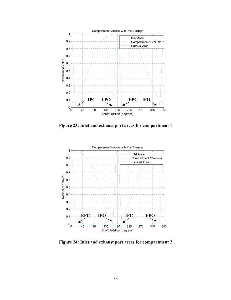
Figure 23: Inlet and exhaust port areas for compartment 1…………………………....33
Figure 24: Inlet and exhaust port areas for compartment 2……………………………33

viii
LIST OF TABLES
Table Page
Table 1: Summary of defining parameters……………………………………………14
Table 2: Summary of device variables………………………………………………..26
Table 3: Coefficients for two-term Fourier series curve fit of volume data………….31

1
CHAPTER 1
INTRODUCTION
1.1 Background
In recent years there has been a significant increase in awareness about how the
daily activities of human beings are impacting the environment. The ecological disaster
that resulted from the Deepwater Horizon incident in the Gulf of Mexico is a startling
example of the unintended consequences of increased global energy demand. Increasing
demand for oil and other fossil fuels from developing Third World nations such as India
and China will continue to force corporations to undertake riskier operations such as
drilling for oil in ever increasing ocean depths. Despite the recent economic downturn,
total worldwide energy demand is expected to increase 49% by the year 2035. [1]
Countries that are not members of the Organization for Economic Cooperation and
Development, such as China and India, are expected to see demand increase by 84%. [1]
A number of conflicting opinions exist as to the actual severity of the current energy
situation; however, there is a consensus that at some point, whether it is in twenty years
or 2000 years, the world will exhaust its remaining fossil fuel deposits. This fact presents
a significant opportunity for the development of new and innovative alternative energy
technologies to help mitigate the effects of increasing energy demands and decreasing
fossil fuel supplies.
Alternative energy is not a new concept. The Dutch have used windmills for
centuries to harness the abundant wind the country experiences. The United States
constructed numerous dams during the Great Depression to extract electricity from
hydropower. Today there are six main alternative sources of energy that are receiving

2
increased attention: solar, hydro, wind, nuclear, bio-fuels and geothermal. All of these
options have their own unique benefits and drawbacks. Within these six options, the two
sectors with the most momentum and growth potential are solar and wind energy. One
driving force behind the recent alternative energy push is an agreement in the
international community to reduce greenhouses gases to levels 80 percent lower than they
were in 1990. [3] One of the biggest benefits of solar energy is that the sun provides the
Earth with what is essentially a limitless supply. Every hour the Sun provides the Earth
with enough energy to satisfy the needs of human civilization for an entire year. [9] The
main drawback to solar energy is finding a way to efficiently capture and convert this
solar radiation. Wind energy presents a different set of problems. Power is generated
through the use of large turbines, often times over 200 feet in diameter. This technology
presents significant mechanical issues in regards to the very large gear systems that are
connected to the turbine blades to generate electricity. Due to their size, they are difficult
to maintain and can suffer catastrophic failures. Furthermore, the actual operation of
these turbines is widely reported to be an annoyance to residents living in their vicinity
due to the noise they generate during windy conditions. For these reasons, solar energy
has become a very attractive option.
Within the solar energy sector there are two methods of collecting sunlight for the use of
generating electricity. The first method does so directly by using photovoltaic (PV) cells
made from silicon and other semi-conductor materials. The main benefit of this
technology is the relatively small amount of extra infrastructure required to implement
the system. PV panels can be purchased and installed fairly easily on a home or
commercial building. The main drawback is that PV systems can only achieve about 10-

3
20% efficiency when converting solar radiation into electricity. [4] This results in costs
that range from 18 to 31 cents per kilowatt-hour for electricity generated on the utility
scale, plants that produce at least 1 megawatt of electrical output. This is significantly
greater than the 11-15 cents per kilowatt-hour for electricity generated by a solar thermal
system on the same scale. [5] Another drawback for PV systems is that they store
electricity directly which is not nearly as efficient as the storage of heat in a solar thermal
system.
The benefits of solar thermal technology, also referred to as concentrating solar
thermal (CST), are numerous. Most importantly, CST systems are capable of achieving
higher overall system efficiencies due to how they convert solar energy into electricity.
[4] Unlike PV cells which convert solar radiation directly into electricity by a chemical
reaction involving electron movement in the materials, CST systems use mirrors to direct
sunlight at a focal point to heat up a working fluid such as water. This fluid is then used
to generate electricity from a power cycle, most typically a Rankine cycle. The latent heat
that remains in the fluid after it undergoes a controlled expansion can be used to heat
water storage tanks or for space heating purposes in a home. These added utilizations of
the captured solar energy are what allow CST systems to have significantly higher overall
system efficiencies than their PV cell counterparts. Another benefit to CST is that the
power cycle technology is the same as what is used in coal burning power plants. The
two main crossover components are the heat exchanger and pump. Even though a greater
number of parts are needed to implement the CST system compared to PV panels, they
are fairly inexpensive because of their prevalence.

4
Recently, solar thermal technology has seen a significant increase in activity on
the utility scale. For the purpose of this research, utility scale will be defined as a system
that generates at least one megawatt of electrical output and small scale will be defined as
generating anything under 25 kilowatts of electrical output. This project will attempt to
develop technology on an even smaller, residential scale of one to three kilowatts, enough
to satisfy the needs of a single, typical U.S. household. The recent increase of activity on
the utility scale has been due to the ability of startup companies like eSolar to accurately
track the sun using sophisticated computer programming. This has allowed the use of flat
mirrors that are inexpensive to manufacture and install compared to the curved mirrors
that are used in parabolic troughs to concentrate sunlight in a CST system. [3] With
improved tracking capabilities, electricity generated from a CST installation is getting
closer to competing with the price of electricity generated by coal. Estimates show that a
kilowatt-hour of electricity delivered from a coal burning power plant costs from 6 to 13
cents on average in the continental United States compared to 11-15 cents from a solar
thermal power plant. [5]
There are a number of reasons as to why solar thermal has not experienced the
same increase in activity on the smaller scale. One of the biggest reasons is the lack of
devices that are currently available to expand the working fluid of the system in a cost
effective manner. Micro-turbines do not scale down well below about 20-25 kW of
output. For this reason, it is not practical to design a system with this type of device
because the output is significantly greater than the needs of a single household. Two
other devices, which are investigated further in the following literature review, are
capable of generating the desired amount of electricity for a single household but have

5
drawbacks due to their tolerances. The tight machining tolerances contribute significantly
to the overall cost of the system. Another concern with all of the potential expansion
devices is to design them in such a way that they can be easily coupled to an electric
generator. This requires limiting their rotational speeds to around 3000 rpm. If further
work is done to develop a better device for expansion on this scale, the benefits of large
scale CST installations could be realized for residential homes and there would be a
realistic renewable energy option for individual homeowners instead of just installing a
few PV panels.
1.2 Literature Review
1.2.1 Small scale systems and expansion devices
A small scale system proposed by Zhai, Dai, Wu and Wang [2] was used as the
primary foundation for the system that includes the small scale expander in this research.
Zhai’s system was designed to generate sufficient electrical and cooling output for small
communities in remote areas. The specific location for the case study the authors carried
out was the Gansu province in northwestern China. The authors designed and analyzed a
hypothetical system that used parabolic trough collectors in the power cycle that can be
seen in Figure 1.

6
Figure 1: Small scale solar thermal system proposed by Zhai, et al [2]
The main purpose of reviewing this system was to study its use of a screw
expander to generate the electricity. The system proposed by Zhai et al [2] claims to be
able to produce 23.5 kW of electric power and 79.8 kW of cooling with a collector area
of 600 m2 and solar radiation of 600 W/m2 in the Gansu region. This system suggests that
a screw expander is capable of operating in a small scale solar thermal application, but it
comes at a large upfront commitment in capital cost. Zhai estimates that the expander
would account for about 20% of the initial capital investment for the system. [2] Any
single component that accounts for such a large portion of the overall system cost has the
opportunity for significant technological improvement to decrease the investment.
If any renewable energy system is to make a notable impact in the future, the
economics will have to be reasonable. Any system that is designed for individual
residential use will have to have a payback period significantly less than the length of the
mortgage of the home in order for the technology to gain real traction and support in the
renewable energy market. Zhai found that the payback period was 18.64 years for interest
rates and energy prices in 2008. However, this payback period decreases significantly

7
with an increase in energy prices or a decrease in the interest rate. Since the time when
the article was published, interest rates have decreased significantly and energy prices
will eventually increase at some point in the future. This article illustrated that now is the
perfect time for investment in renewable energy because the financing for the
construction of systems can be done now while interest rates are favorable and the benefit
will be exaggerated further when energy prices increase. Zhai’s analysis showed that a
50% increase in energy prices would reduce the payback period to less than 10 years,
well under the typical mortgage length.
The technology and operating principles behind the screw expander used in the
system described by Zhai et al are explained further through the work of Kovacevic,
Stosic, and Smith. The screw expander is a positive displacement rotary machine that
uses a pair of meshed helical rotors. A drawing of the screw expander can be seen in
Figure 2. Two of the major drawbacks of this type of expansion device are the machining
tolerances required for the smooth operation of the meshed gears and the bearing forces
in the device. The clearance required between the two gears in this particular device is
30-50 µm. Even with advances in high-accuracy profile milling that have decreased the
cost of machining significantly, it would still be advantageous from a cost and
operational standpoint to use a device that requires less machining precision. Another
problem with the screw expander is the handling of the large bearing forces that are
generated during operation.

8
Figure 2: Screw expander described by Kovacevic et al [6]
Another device capable of expanding a working fluid on the proper scale for this
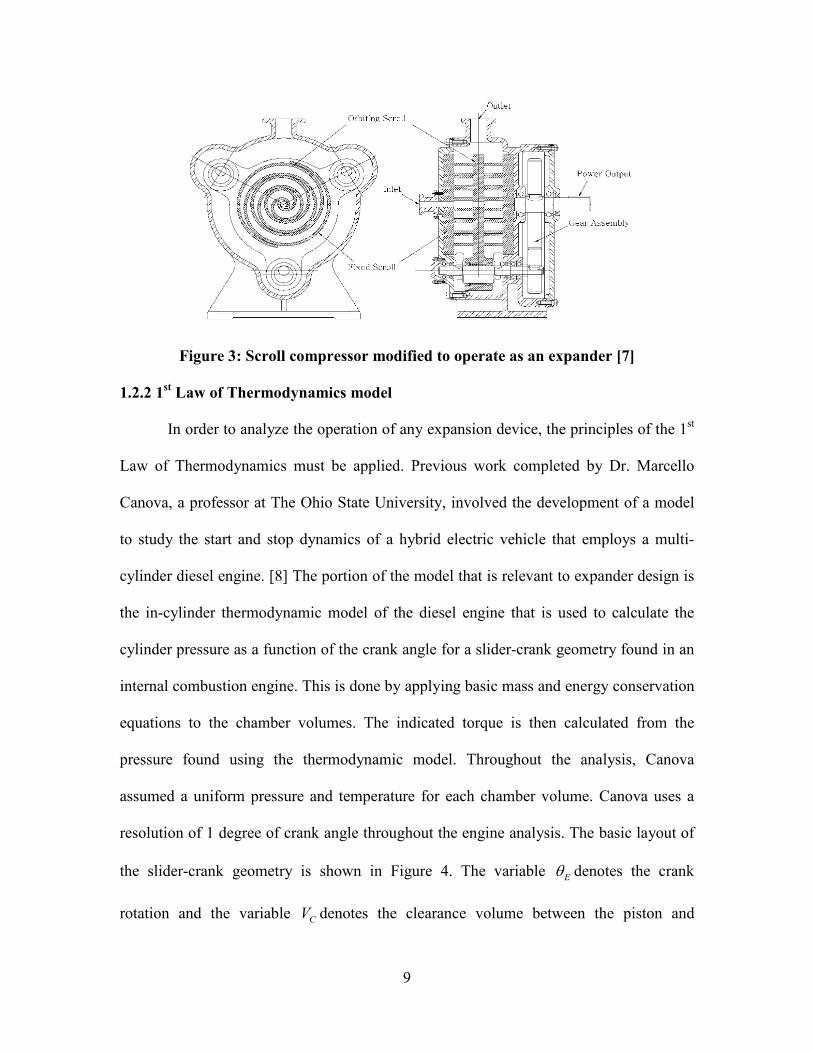
project is a scroll compressor modified to run as an expander. A diagram of such a device
developed by Kim, Ahn, Park and Rha [7] is given in Figure 3. This device was used for
power generation from a low-temperature steam source. Similar to the previously
mentioned screw expander, this device also required extremely close machining
tolerances for efficient operations. The clearance between the fixed and orbiting scrolls
was 64 µm and the authors suggest reducing that value by half to increase the volumetric
and total efficiencies. These extreme tolerances between the fixed and orbiting scrolls are
needed to limit the leakage flow between the high and low pressure chambers.
9
Figure 3: Scroll compressor modified to operate as an expander [7]
1.2.2 1st Law of Thermodynamics model
In order to analyze the operation of any expansion device, the principles of the 1st
Law of Thermodynamics must be applied. Previous work completed by Dr. Marcello
Canova, a professor at The Ohio State University, involved the development of a model
to study the start and stop dynamics of a hybrid electric vehicle that employs a multi-
cylinder diesel engine. [8] The portion of the model that is relevant to expander design is
the in-cylinder thermodynamic model of the diesel engine that is used to calculate the
cylinder pressure as a function of the crank angle for a slider-crank geometry found in an
internal combustion engine. This is done by applying basic mass and energy conservation
equations to the chamber volumes. The indicated torque is then calculated from the
pressure found using the thermodynamic model. Throughout the analysis, Canova
assumed a uniform pressure and temperature for each chamber volume. Canova uses a
resolution of 1 degree of crank angle throughout the engine analysis. The basic layout of
the slider-crank geometry is shown in Figure 4. The variable Eθ denotes the crank
rotation and the variable CV denotes the clearance volume between the piston and

10
cylinder at full extension. These variables are used to develop a function for the volume
of working fluid in the cylinder at any given crank rotation.
Figure 4: Slider-crank geometry for IC engine
Equation 1 shows the basic energy balance used in the thermodynamic model
where U is the internal system energy, Qg is the heat from combustion, Qw is the heat loss
through the cylinder walls and V is the cylinder volume. All of these values are a
function of the crank angle Eθ .
g w
E E E E
dQdU dQ dVp
d d d dθ θ θ θ= − − (1)
Canova has taken the working fluid in the thermodynamic model of the engine to
be air. As a result, Equation 1 is modified by combining it with the ideal gas law using
constant specific heats in Equation 2. The ratio of specific heats is denoted by γ.
( )1 g
E E E
dQdp p dVd V d V d
γγ
θ θ θ−
= − + (2)
For the purpose of this research, the last term in Equation 2 is neglected because
there is no combustion portion of the cycle in the solar thermal application and it has
been assumed that there is no significant heat loss to the ambient. When this term is
removed, the differential equation that is used to solve for the chamber pressure at any
given crank angle is given by Equation 3.

11
E E
dp p dVd V d
γθ θ
= − (3)
The volume function for a slider-crank, while not simple, is defined analytically
by Canova. The geometry of the proposed expander in this research is much more
complex and requires the compartment volume function to be defined numerically to
carry out the appropriate analysis according to the 1st Law of Thermodynamics.
1.3 Motivation
This project was undertaken because of the current opportunity for development
in the residential renewable energy market. The lack of expansion devices available for
generating electricity in a cost effective manner on a residential scale is considered a
gaping hole that needs to be filled if the global community is serious about solving the
current energy situation. In that same light, a secondary motivation for this project was to
develop a technology that could have a significant economic impact for the United States.
Renewable energy has the potential to be the economic savior of the 21st century through
job creation in a new economic sector. A number of European countries have already
realized this fact as Spain and Germany are global leaders in the solar energy field. The
biggest downfall of renewable energy is the upfront cost required to implement these
types of systems. The expander is a significant portion of this cost as it can account for up
to 25-30% of the overall system cost [2]. The theoretical expander put forth in this project
has the potential to enable the development of cost-effective solutions for providing clean
energy for future generations
1.4 Project Objective
The objective of this project was to gain an understanding of the operation for a
proposed expander and to develop a methodology for 1st Law of Thermodynamic

12
analysis. The methodology and analysis will ultimately be used to quantify the potential
electrical output of the device. The work was done as a portion of a larger project to
develop a residential solar thermal power generation system. The other two parts of the
research involved the development of a solar collection system and a parametric analysis
of the overall system which involved exploration of potential working fluids and
operating conditions (pressure, temperature, etc.) for a residential scale system. This
work was completed by Michael Nesteroff and Jake Wither respectively.

13
CHAPTER 2
PROPOSED EXPANSION DEVICE
In this section the design of the proposed expansion device is described in detail
in order understand its geometry and motion. This information was used to develop the
necessary functions and methodology for analysis according to the 1st Law of
Thermodynamics analogous to what is done for an internal combustion engine. For this
particular device, the geometry and motion are much more complex than the slider-crank
geometry found in an IC engine. The increased complexity required extensive work to
gain the necessary understanding for development of the volumetric functions needed for
the thermodynamic analysis. This device was originally designed by Dr. Codrin-Gruie
Cantemir, a Center for Automotive Research Chief Designer at The Ohio State
University. The proposed device was originally designed to work in the context of a
waste heat recovery system for an automobile. As such, the device size and operating
conditions were not initially optimized for the application of a residential solar thermal
power generation system.
2.1 Conceptual Design
The expander is an assembly of four individual components. To aid in the
referencing of these components, a consistent nomenclature has been defined. The four
parts are the shell, piston, follower and shaft. Each of these components will be described
further in the following sections. For any type of expansion device there are two main
parameters that are used to categorize the device: expansion ratio and displacement. Both
of these defining parameters depend on the maximum and minimum compartment

14
volumes which are shown in Figure 5. These volumes are defined as the amount of space
between the purple or pink piston face and the beige shell.
Vmax VminVmax Vmin
Figure 5: Maximum and minimum volumes for defining parameters
The relationships between the maximum and minimum volume for the defining
parameters are summarized in Table 1. The current iteration of the design defines a
device with an expansion ratio of 16 and a maximum displacement of 15 in3. These
values were obtained by assuming a minimum cavity volume of 1 in3. The minimum
cavity volume or clearance volume is shown in the right hand side of Figure 5 when one
side of the piston face is flat against the top of the shell.
Table 1: Summary of defining parameters
Relationship Current Design Result Expansion Ratio Vmax/Vmin 16in3/1in3 16
Displacement Vmax-Vmin 16in3-1in3 15 in3
Once the basic defining parameters of the device were established, the next step
was to understand the motion of the device and how it would function if it were placed in
a power generation cycle. A basic schematic of the device is shown in Figure 6 to aid in

15
the explanation of how the working fluid interacts with the ports of the device and the
output shaft rotation, θ. The working fluid, which has been assumed to be air for this
research, enters the inlet opening at an elevated energy state (high temperature and high
pressure). It enters the compartment as the inlet port is uncovered by the shell (teal
component in Figure 6) due to the shaft rotation (green arrow in Figure 6). After the
compartment has been completely filled with air, the rotation of the piston closes the inlet
port in a manner similar to how it was opened. This isolates the high energy air in the
compartment to undergo an expansion as the volume in the compartment increases due to
the previously described shaft rotation. As the compartment approaches its maximum
volume, the exhaust port begins to open using the same “uncovering” method seen with
the inlet. At this point, the air, which is now at a lower temperature and pressure, begins
to flow out of the device. This process is repeated for both of the compartments shown in
Figure 6 defined by the volume between the purple and pink piston face and beige shell.
Figure 6: Inlet and exhaust ports of expansion device

16
2.2 Three-Dimensional Model of Current Design Iteration
In order to gain a better understanding of the expander motion that was described
in the previous section, a three-dimensional model of the device was created using three-
dimensional printing. This prototype was strictly meant for conceptualization and is not
meant to be used in an actual system.
2.2.1 Shell
The largest component in the assembly is the shell. This component was designed
as a modified hemisphere to allow for the rotational motion of the piston. The three
dimensional model of the shell can be seen in Figure 7. The opening in the side of the
shell is one of the two ports. As previously mentioned, these openings act as the inlet and
exhaust ports of the device. A number of modifications including size, shape and
positioning of the ports relative to each other and to the shell can be made in the future in
order to optimize the device performance.
Figure 7: 3D model of shell component
There are three main radii that define the shape and size of the shell. The R, R1
and R2 dimensions seen in Figure 8 define the modified hemisphere. The current iteration
of the design was created by making a hemisphere with radius R equal to 3.94 inches.

17
Two additional radii, R1 and are R2, were set to equal 3.86 and 3.13 inches respectively.
The portions of the hemisphere outside of R1 and R2 were removed and the remaining
shape was revolved about the blue dashed line to create the three dimensional shell that
resembles a bowl. If it is desired to increase the overall size of the device to achieve a
greater power output, one would only need to modify R, R1 and R2 by the same scaling
factor.
R2 R R1R2 R R1
Figure 8: Critical dimensions for shell component
2.2.2 Piston
The piston component is a modified spherical shape with a “wedge” portion of
material removed from each side. The wedge of material is removed so the compartment
of volume between the surface of the piston and the shell is generated when the piston is
placed in the shell. This cavity is what contains the working fluid that is expanded to
generate output power. The surfaces of the piston that form the two volume
compartments are shown as the flat purple and pink surfaces in the device assembly in
Figure 6. The top view for the three dimensional model of the piston is shown in Figure 9
and the side view in Figure 10. The cavity seen in the top view shown by the blue arrow
is made to house the shaft. The two pegs that are extending from the shaft cavity, denoted
by the green arrows, are used to connect to the follower. A more detailed assembly is

18
described in section 2.3. The surface below the pegs and the shaft cavity for is where the
follower is always in contact with the piston. This surface is the back side of the
previously defined piston face. The interaction between this surface and the curved top
edge of the follower is what causes the rotation of the overall device. The piston roughly
traces the red line in Figure 9 when in contact with the follower. The follower is
described further in the following section.
Figure 9: 3D model of piston component
Figure 10: Side view of piston component

19
2.2.3 Follower
The follower controls the motion of the piston in the final assembly. The curved
top edge of the three dimensional model in Figure 11 is always in contact with the piston.
The design of the follower is such that it creates two types of motion when connected to
the piston. The piston rocks back and forth about the axis where the pegs on the piston
connect with to the follower. This is shown by the orange dashed line in Figure 11. The
second motion is what causes the output shaft to rotate. The entire piston, follower and
shaft assembly rotates about the axis illustrated by the green dashed line in Figure 11.
Figure 11: 3D model of follower component
2.2.4 Shaft
The final component of the assembly is the shaft. This portion of the device will
ultimately connect to an electric generator to create an electrical output. The three
dimensional model of this component is seen in Figure 12. The model is a simple T-shape
that combines two cylinders. The cylinder that connects directly to the piston has a radius
of 1.19 inches and is oriented vertically in Figure 12. The cylinder that would connect to
the generator has a radius of 0.65 inches and is oriented horizontally in Figure 12.

20
Figure 12: 3D model of shaft component
2.3 Expansion device assembly
The four components of the device are currently designed so that they can only be
assembled in one specific order. The shaft must first be connected to the piston. This step
is not depicted here because the tolerances of the three dimensional model were not
precise enough to allow the shaft to fit in to the appropriate cavity on the piston. What is
shown in Figure 13 is the second step in the assembly process. In this step the follower is
joined to the piston using the two pegs that were described in the previous section.
Figure 13: Assembly of follower and piston components

21
The third step of the assembly process involves placing the piston/shaft/follower
assembly in the shell. The result of this step, without the shaft, is shown in Figure 14. The
“cap” portion of the shell is missing from this assembly. This portion was excluded
because the three dimensional modeling procedure did not allow the shell to be
constructed as a single piece. In the final assembly, the cap portion of the shell would be
placed over the follower.
Figure 14: Final assembly without the shaft included

22
CHAPTER 3
NUMERICAL EXPERIMENT TO DEFINE SIMULATION FUNCTIONS
This chapter describes the procedure that was used to determine the volume
function for the proposed expander through the use of MATLAB and SolidWorks. The
functions for the area of theoretical inlet and exhaust ports are also included. These
functions were found to facilitate the future calculation of the pressure in each
compartment at any given shaft rotation using MATLAB code that was developed at the
Center for Automotive Research. This code treats the mass entering and leaving the
device as orifice flow through the inlet and exhaust ports. Ultimately, the pressure in each
compartment will be used to calculate the torque acting on the expander which in turn
could be used to predict the potential electrical output of the device when coupled to an
electric generator.
3.1 Numerical Experiment Methodology
An outline of the methodology for the numerical experiment that was used to
establish the compartment volume and port area functions for the expander is shown in
Figure 15. The first step involved defining the design and operational variables for the
shell and the piston. Next, a MATLAB program was written to generate values for the
two variables that were used in SolidWorks to numerically find the compartment volumes
as a function of shaft rotation. The values for the compartment volume that were found
using the SolidWorks model were compiled in an Excel spreadsheet and then imported
into MATLAB for curve fitting purposes. Once an appropriate function was fit to the
volume data, the functions for the inlet and exhaust port areas were defined in MATLAB.
At this point, depending on the results of the simulation that would be run using the

23
orifice flow code developed at the Center for Automotive Research, a new iteration of the
design could be explored by modifying the numerical values of the design parameters and
reverting to the second step in the process.
2. Develop MATLAB code to generate values for variables for
numerical experiment
3. Determine volume values inSolidWorks and compile the data
in Excel spreadsheet
4. Import volume data to MATLAB and curve fit the data
5. Choose appropriateinlet/exhaust port
functions and run simulation
1. Define variables
Figure 15: Outline of procedure used to find volume function
3.2 Variable Definition
The first step in the numerical experiment methodology was defining the
variables of the shell and piston components that would be used throughout the rest of the
analysis. One critical component of the shell design is the angle that the shell “cap”
makes with the y-axis as defined by α in Figure 16 where the shell is the beige portion of
the sectioned final assembly drawing. This angle is determined by the piston design (teal
component in Figure 16) and is used to connect and properly align the piston, follower
(blue) and shaft (black) with the rest of the shell. Points A, B and C are denoted because
the piston must remain in contact with the shell at these three points to maintain the seal
between the two compartments and the outside atmosphere. The other three variables that

24
define the size and shape of the shell are the radii R, R1 and R2 which were previously
mentioned in Chapter 2.
B
C
A
y
x
αR
R1
B
C
A
y
x
αR
R2R1
B
C
A
y
x
αR
R1
B
C
A
y
x
αR
R2
B
C
A
y
x
αR
R1
B
C
A
y
x
αR
R2R1
Figure 16: Static relationships of expansion device assembly
The piston component has a number of geometric relationships shown in Figure
17 that are essential to the functionality and analysis of the expansion device. The most
critical of these is the angle φ that the piston face makes with the shell (dashed white
line). As the shaft rotates, the angle of the piston face varies in a rocking manner similar
to a see-saw. The motion of the piston face differs from a simple pivoting motion in that
both the top and bottom edge of piston face also exhibit some translational motion along
the top and sides of the shell at the points of tangency. Based on the geometry in the
current design, the rocking causes the angle of the piston face to vary between a
minimum of 0 degrees, when it is flat against the top of the shell and 40 degrees when the
other piston face is flat against the top of the shell. This angle was assumed to vary
according to a simple periodic sine function between the minimum and maximum values.
25
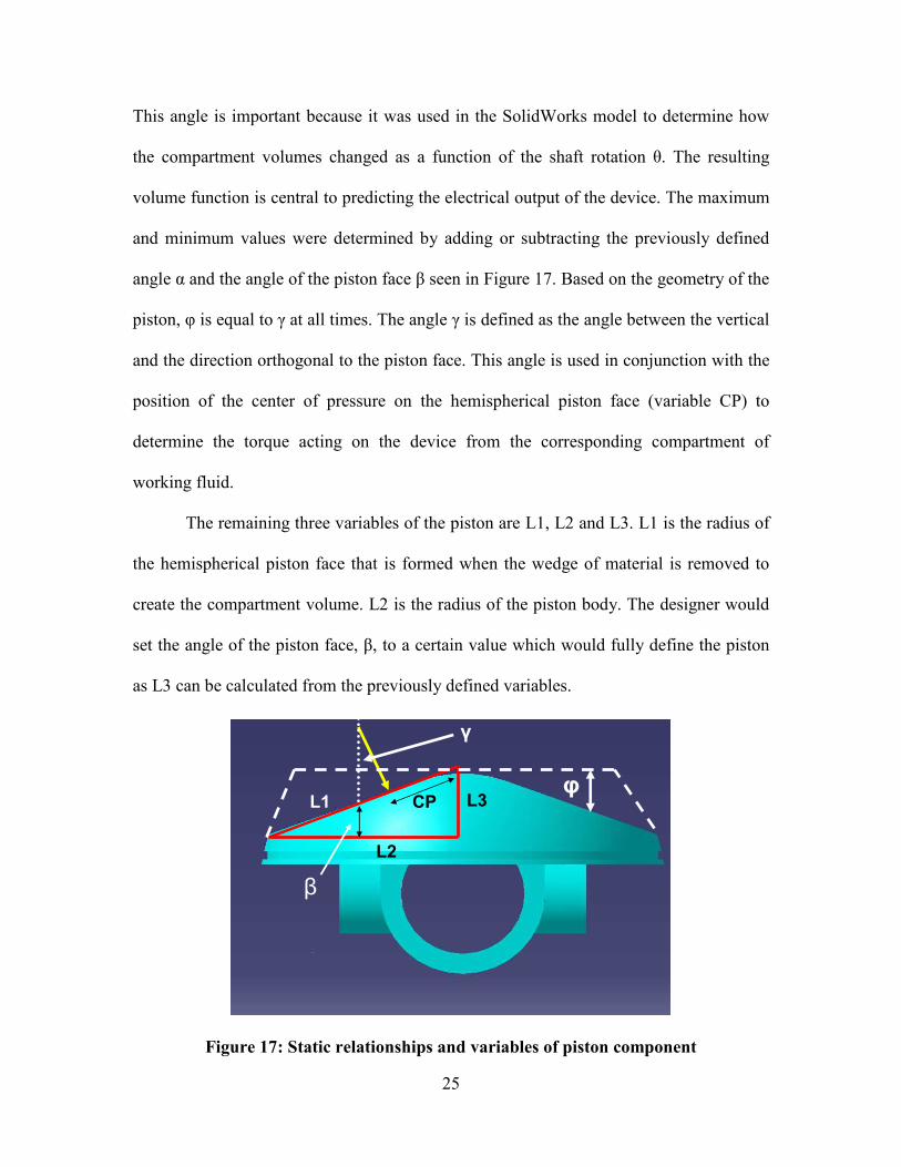
This angle is important because it was used in the SolidWorks model to determine how
the compartment volumes changed as a function of the shaft rotation θ. The resulting
volume function is central to predicting the electrical output of the device. The maximum
and minimum values were determined by adding or subtracting the previously defined
angle α and the angle of the piston face β seen in Figure 17. Based on the geometry of the
piston, φ is equal to γ at all times. The angle γ is defined as the angle between the vertical
and the direction orthogonal to the piston face. This angle is used in conjunction with the
position of the center of pressure on the hemispherical piston face (variable CP) to
determine the torque acting on the device from the corresponding compartment of
working fluid.
The remaining three variables of the piston are L1, L2 and L3. L1 is the radius of
the hemispherical piston face that is formed when the wedge of material is removed to
create the compartment volume. L2 is the radius of the piston body. The designer would
set the angle of the piston face, β, to a certain value which would fully define the piston
as L3 can be calculated from the previously defined variables.
β
L1
L2
γ
L3CPφ
β
L1
L2
γ
L3CPφ
β
L1
L2
γ
L3CPφ
Figure 17: Static relationships and variables of piston component
26
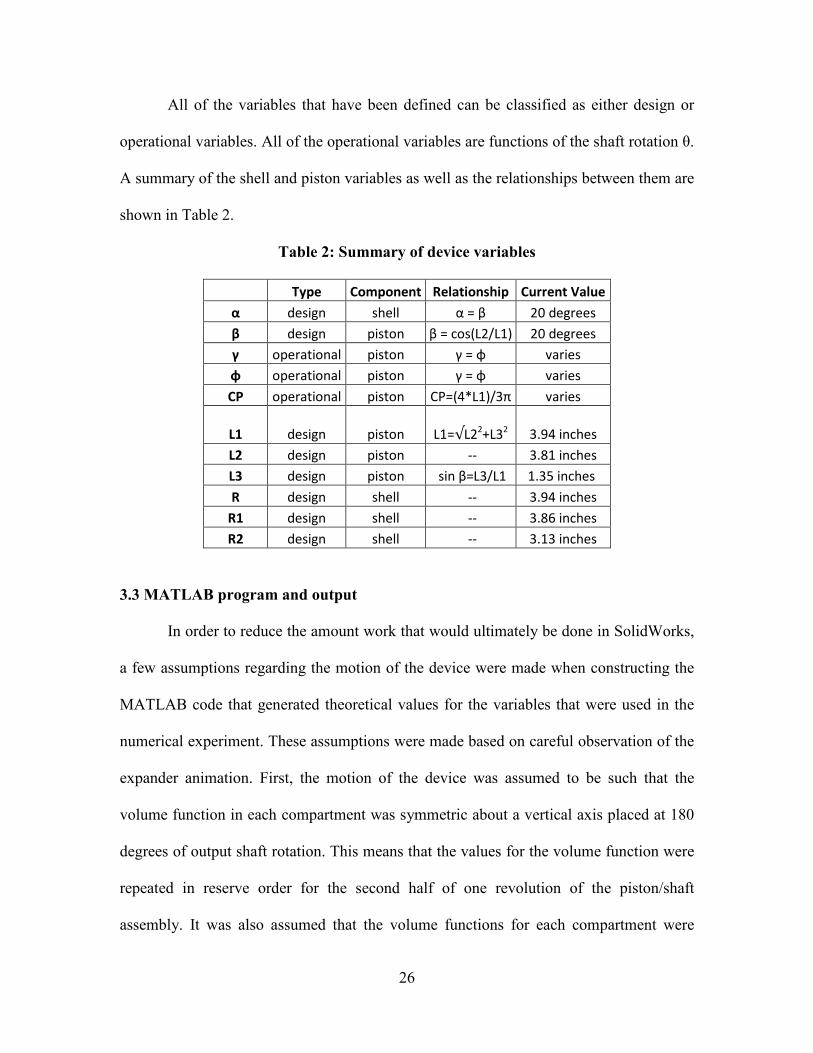
All of the variables that have been defined can be classified as either design or
operational variables. All of the operational variables are functions of the shaft rotation θ.
A summary of the shell and piston variables as well as the relationships between them are
shown in Table 2.
Table 2: Summary of device variables
Type Component Relationship Current Value α design shell α = β 20 degrees β design piston β = cos(L2/L1) 20 degrees γ operational piston γ = φ varies φ operational piston γ = φ varies CP operational piston CP=(4*L1)/3π varies
L1 design piston L1=√L22+L32 3.94 inches L2 design piston -- 3.81 inches L3 design piston sin β=L3/L1 1.35 inches R design shell -- 3.94 inches
R1 design shell -- 3.86 inches R2 design shell -- 3.13 inches
3.3 MATLAB program and output
In order to reduce the amount work that would ultimately be done in SolidWorks,
a few assumptions regarding the motion of the device were made when constructing the
MATLAB code that generated theoretical values for the variables that were used in the
numerical experiment. These assumptions were made based on careful observation of the
expander animation. First, the motion of the device was assumed to be such that the
volume function in each compartment was symmetric about a vertical axis placed at 180
degrees of output shaft rotation. This means that the values for the volume function were
repeated in reserve order for the second half of one revolution of the piston/shaft
assembly. It was also assumed that the volume functions for each compartment were

27
identical and simply out of phase by 180 degrees meaning that when one of the
compartments was at a maximum volume the second compartment was at a minimum
volume.
The behavior of h and φ based on the MATLAB code developed from these
assumptions is shown in Figures 18 and 19. The height, h, was taken as the vertical
distance between the top of the shell and the bottommost edge of the piston. It was
calculated by multiplying the radius of the piston by the sine of the angle φ. The values
have been normalized to show the general behavior of these variables. For this design
iteration, the piston face angle varies sinusoidal between 0 and 40 degrees and the height
varies between 0 inches when the piston face angle is 0 degrees and about 2.6 inches
when that angle is 40 degrees. These are the values that were used in SolidWorks to
define the position of the cutting plane that was used to modify the shell volume for
finding the compartment volume.
Figure 18: Piston face angle versus shaft rotation
0 45 90 135 180 225 270 315 3600
0.1
0.2
0.3
0.4
0.5
0.6
0.7
0.8
0.9
1
Output shaft rotation (degrees)
Nor
mal
ize
d P
isto
n F
ace
Ang
le (p
hi/p
him
ax)
Relationship between Piston Face Angle and Output Shaft Rotation
Compartment 1Compartment 2

28
Figure 19: Normalized height versus shaft rotation
3.4 SolidWorks Modeling
After computing values for h and φ in MATLAB, the next step for finding the
volume functions in SolidWorks was to recreate the shell component using the procedure
shown in Figure 8 of Chapter 2. A set of screen captures from SolidWorks are shown in
Figure 20 to illustrate the procedure that was used to find the compartment volume once
the shell was recreated. In short, the location of a cutting plane was defined by creating a
triangle from three values. Two of these values, h and φ, vary due to the rocking motion
of the piston. The third value, L1, is constant because it defines the radius of the piston
face. Taken together, this causes the angle of the piston face to change and the points of
tangency (ends of the blue line in Figure 20) to translate along the top and ride side of the
shell volume.
Once the shell volume was created, a vertical line of length h, as determined by
MATLAB program, was drawn from the top of the shell volume downward. The
0 45 90 135 180 225 270 315 3600
0.1
0.2
0.3
0.4
0.5
0.6
0.7
0.8
0.9
1
Output shaft rotation (degrees)
Nor
mal
ize
d H
eigh
t (h/
hmax
)
Relationship between Cut Height and Output Shaft Rotation
Compartment 1Compartment 2

29
normalized value that was previously described for the height was multiplied by a scaling
factor of 2.6 inches to represent the current design. Where this line ended, a horizontal
line was drawn to connect with the edge of the shell volume. Once this point was located,
the cutting plane line, which also represents the position and orientation of the piston face
in the shell, was drawn at the angle φ, as determined by the MATLAB program, and was
extended at that angle until it intersected with the top of the shell. The normalized value
for the angle was multiplied by a scaling factor of 40 because the maximum value for this
angle in the current design is 40 degrees. This line was then used to make an extruded cut
of the volume below the cutting plane with the remaining volume being the desired
compartment volume. This process was repeated for values of h and φ at every five
degrees of output shaft rotation
3φ
2φ2h
3h
3φ
1h1φ
L1
L1
3φ
2φ2h
3h
3φ
1h1φ
L1
L1
Figure 20: Variable definition for finding volume function in SolidWorks

30
3.5 Curve fitting volume data
A plot of the volume data that was compiled from the SolidWorks model is shown
in Figure 21. Again this data has been normalized by dividing the measured volume (V)
by the maximum cavity volume for this particular iteration of the design (15 in3). This
was done in order to understand the fundamental pattern of the volume function. It is
clear from this plot that the volume function is periodic, but it is not a simple sine or
cosine function.
Figure 21: Volume function taken numerically from SolidWorks
In order to smooth out the inaccuracies from the numerical method that was
originally used to find the volume, the volume data was fit using a two-term Fourier
series in MATLAB. A plot of the curve fit is shown in Figure 22. A summary of the
coefficients for the two-term Fourier series can be found in Table 3. The values from the
curve fit shown in Figure 22 were the final values that would be used in the simulation to
predict the pressure inside each compartment and the resulting torque.
0 45 90 135 180 225 270 315 3600
0.1
0.2
0.3
0.4
0.5
0.6
0.7
0.8
0.9
1Volume Function
Shaft Rotation (degrees)
Nor
mal
ized
Cav
ity V
olum
e (V
/Vm
ax)
Compartment 1Compartment 2

31
Figure 22: Two-term Fourier series fit of volume functions
Table 3: Coefficients for two-term Fourier series curve fit of volume data
Compartment 1 Compartment 2 a0 0.5929 0.5923 a1 -0.4991 0.4979 a2 0.003974 0.008551 b1 -0.09433 -0.09289 b2 0.001502 -0.003192 w 0.01741 0.01755
General Equation: f(x) = a0 + a1*cos(w*x) + a2*sin(w*x) +b1*cos(2*x*w) + b2*sin(2*x*w)
3.6 Inlet and exhaust port functions
The second set of functions that needed to be defined in order to predict the
internal compartment pressure and the resulting torque was how the area of the inlet and
exhaust ports of the expander varied as a function of the shaft rotation. The flow of the
working fluid through these ports is treated as orifice flow in the simulation. The original
expander design included an inlet and exhaust port. However, these ports had not been
0 45 90 135 180 225 270 315 3600
0.1
0.2
0.3
0.4
0.5
0.6
0.7
0.8
0.9
1
Shaft Rotation (degrees)
Nor
mal
ized
Cav
ity V
olum
e (V
/Vm
ax)
Volume Function Curve Fit

32
optimized in terms of location, shape or size. In order to maximize the potential output of
the expander, functions for exposed area of the theoretical inlet and exhaust ports were
created. The duration of the opening and closing as well as where these events were
positioned during the course of one shaft revolution were chosen in order to maximize the
output of the expander. The inlet port for compartment 1 begins to open at 340 degrees
when the volume is near a minimum. It reaches its maximum area at 360 or 0 degrees and
is closed by 20 degrees of shaft rotation. All told, the opening and closing of the inlet and
exhaust port takes 40 degrees of shaft rotation. The duration of the opening and closing of
the ports was based on what is common for cylinders in internal combustion engines.
This was done to maximize the time when the working fluid is isolated in the
compartment while the volume is increasing. This allows the device to extract more work
during the cycle. The exhaust port follows the same pattern as the inlet with the only
difference being that it starts opening at 160 degrees of shaft rotation and is closed by 200
degrees of rotation. At every other time besides during the periods mentioned, the ports
are closed. A plot of the port area for compartment 1 is shown in Figure 23. The plot for
the port areas of compartment 2 are shown in Figure 24. Again, due to the assumptions
that were originally made about the motion of device, these functions were chosen to be
identical but out of phase by 180 degrees to those for compartment 1. In these figures, the
timing of the ports is denoted by IPO (intake port opening), IPC (intake port closing),
EPO (exhaust port opening) and EPC (exhaust port closing).
33
Figure 23: Inlet and exhaust port areas for compartment 1
Figure 24: Inlet and exhaust port areas for compartment 2
0 45 90 135 180 225 270 315 3600
0.1
0.2
0.3
0.4
0.5
0.6
0.7
0.8
0.9
1
Shaft Rotation (degrees)
Nor
mal
ize
d V
alue
Compartment Volume with Port Timings
Inlet AreaCompartment 2 VolumeExhaust Area
0 45 90 135 180 225 270 315 3600
0.1
0.2
0.3
0.4
0.5
0.6
0.7
0.8
0.9
1
Shaft Rotation (degrees)
Nor
mal
ize
d V
alue
Compartment Volume with Port Timings
Inlet AreaCompartment 1 VolumeExhaust Area
EPO EPC IPO IPC
EPO EPC IPO IPC

34
CHAPTER 4
ORIFICE FLOW FOR SIMULATION
This chapter explains the orifice flow equations that utilize the port area functions
that were defined in Chapter 3. The simulation developed at the Center for Automotive
Research that will be used to predict the instantaneous compartment pressure and torque
combines the orifice flow equation presented here with the mass and energy balance
shown in Chapter 1 to carry out the 1st Law of Thermodynamic analysis. The actual
simulation has not been carried out for this research. However, the equations and range of
parameters are given here.
4.1 Orifice flow equation
The orifice flow equation that will be used to simulation the working fluid
entering and exiting the expander is based on an intake manifold of an IC engine. There
are two conditions for the orifice flow, un-choked and choked. The equation for un-
choked flow is given in Equation 4 and the equation for choked flow is given in Equation
5. The conditions for determining whether the flow is un-choked or choked are also
shown.
1 1
1, , ,
,2 2
1 if 1 1
a IM a IM a IMd amba th
amb amb ambamb
p p pC Apm
p p pRT
γ γγ γ γγ
γ γ
−
−
= − ≥ − +
�
� � (4)
11 1
,,
2 2 if
1 1a IMd amb
a th
ambamb
pC Apm
pRT
γ γγ γ
γγ γ
+− −
= ⟨ + +
�
� � (5)

35
In these equations, the most important variables are pamb, pa,IM, A and ma,th. The
variable A represents the exposed area of the inlet or exhaust port. The port area
functions that were defined in the previous chapter will be used to supply values for this
variable. The ma,th variable represents the mass of working fluid, assumed to be air for
this research, entering the expander. The amount of fluid entering the compartment will
vary depending on the ambient pressure, pamb, the instantaneous compartment pressure,
pa,IM, and the port area. For this particular device, it is assumed that the flow of working
fluid will start choked when the port area first begins the open and the pressure ratio
between the ambient and compartment is high. The flow will evolve to being un-choked
when the area opens and the pressure ratio begins to equalize as the compartment
pressure begins to reach the same value as the upstream supply pressure.
4.2 Simulation parameters
The three main parameters for the simulation that are taken from this portion of
the residential solar thermal research are the expansion ratio, volume functions and port
area functions. The volume function will be dependent on the expansion ratio and
displacement. A realistic range for the expansion ratio is between 2 and 20. It is desired
to design for an expansion ratio at the upper end of that range in order to maximize the
potential output of the expander. For this reason, the expansion ratio is currently set to 16.
The other parameters for the simulation such as mass flow, temperatures, and pressures
were explored in the parametric analysis completed by Jake Wither. [10] In order to
develop a successful set of simulation conditions for the system, the work presented here
should be combined with the range of variables explored by Wither.

36
CHAPTER 5
SUMMARY AND FUTURE WORK
In this thesis, an innovative expander for the purpose of residential solar thermal
power generation was described. The basic understanding of its motion and functionality
in a power cycle was developed by careful examination of device animations and by the
creating a three-dimensional model of the current expander design to visual how all of the
expander components fit and moved together. This understanding was used to develop a
methodology for completing analysis according to the 1st Law of Thermodynamics. The
analysis for this particular device is very similar to that of an internal combustion engine
but with a much more complex geometry. The increased in geometry complexity meant
that the necessary functions for the thermodynamic analysis could not be defined
analytically and a numerical method using MATLAB code and SolidWorks procedure
was created.
The next step for this research would be to develop an experiment to explore a
range of variables in the simulation that utilizes the functions defined in this research.
After compiling the potential output of the device from the simulation the necessary
design changes should be made so that the expander can reach the desired output of 1-3
kW. These design alterations will mainly involve scaling and incorporating the
theoretical port design into an actual CAD model. Once the design is completed, a
functioning prototype should be constructed from a material such as aluminum or some
other metal that is easy to machine and can withstand elevated temperatures and
pressures. Testing on this device should first be done isolated from an actual power cycle
to verify the volume, pressure and torque values that were predicted in the simulation. At

37
this point the sealing concerns regarding the seal between the compartments and between
the piston and shell will be addressed. The final step in the process will be to place the
functional expander prototype in a residential power generation system to determine its
viability as a business proposition.

38
BIBLIOGRAPHY
[1] U.S. Energy Information Association. International Energy Outlook 2010.
http://www.eia.doe.gov/oiaf/ieo/highlights. 2010.
[2] H. Zhai, Y.J. Dai, J.Y. Wu, R.Z. Wang. Energy and exergy analyses on a novel
hybrid solar heating, cooling and power generation system for remote areas.
Applied Energy, 86:1395-1404. 2009.
[3] David Roberts. The Future of Energy: Solar Power. Popular Science,
275 (1): 39-47. 2009.
[4] George Johnson. Plugging into the Sun. National Geographic, 216 (3): 28-53.
2009.
[5] M.A. Schilling, M. Esmundo. Technology S-curves in renewable energy
alternatives: Analysis and implications for industry and government. Energy
Policy, 37 (5): 1767-1781. 2009.
[6] N Stosic, I K Smith, A Kovacevic. Opportunities for innovation with screw
compressors. Proc. Instn Mech. Engrs Part E: J. Process Mechanical
Engineering, 217: 157-170. 2003.
[7] H J Kim, J M Ahn, I Park, P C Rha. Scroll expander for power generation from a
low-grade steam source. Proc. Instn Mech. Engrs Part A: J. Power and Energy,
221: 705-712. 2007
[8] Marcello Canova, Yann Guezennec, Steve Yurkovich. On the Control of Engine
Start/Stop Dynamics in a Hybrid Electric Vehicle. Journal of Dynamic Systems,
Measurement, and Control, 131: 1-12. 2009.

39
[9] United Press International Inc. How much solar energy hits Earth. EcoWorld,
www.ecoworld.com/energy-fuels/how-much-solar-energy-hits-earth. 2006.
[10] Jake Wither. Numerical Analysis of Residential Electricity Generation Using
Solar Thermal Energy. Undergraduate Honors Thesis, The Ohio State University,
November 2010.


![Expander 符号生成行列、パリティ検査行列、Tanner グラフ expander 符号 expander グラフ [Sipser-Spieleman ‘96] expander 符号の構成 bit-flipping 復号法](https://cdn.vdocument.in/doc/165x107/5f0bdbc37e708231d4328ff6/expander-c-ceoefffoeeoetanner-ff-expander.jpg)


