EVMS
1
Analysisof
Earned Value Data
In Depth Training for EV Analysts
Eleanor HauptASC/FMCE

EVMS
2
Questions to be Answered
Are we on schedule?Are we on cost?What are the significant variances? Why do we have variances?Who is responsible?What is the trend to date?
Are we on schedule?Are we on cost?What are the significant variances? Why do we have variances?Who is responsible?What is the trend to date?
When will we finish? What will it cost at the end? How can we control the trend?
When will we finish? What will it cost at the end? How can we control the trend?
We analyze the past performance………to help us control the future
PAST PRESENT FUTURE
EVMS
3
Analysis Roadmap
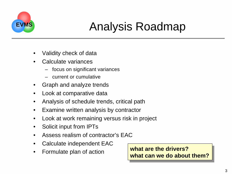
• Validity check of data• Calculate variances
– focus on significant variances– current or cumulative
• Graph and analyze trends• Look at comparative data• Analysis of schedule trends, critical path• Examine written analysis by contractor• Look at work remaining versus risk in project• Solicit input from IPTs• Assess realism of contractor’s EAC• Calculate independent EAC• Formulate plan of action what are the drivers?
what can we do about them?what are the drivers?what can we do about them?

EVMS
4
Validity Check of Data
• Elements on report should total properly– Total BAC should equal CBB (compare to contract)– Format 1 totals should match Format 2 totals– Refer to AFMCPAM 65-501 for further checklists
• Are variances that meet the reporting threshold explained in Format 5?• For any element:
– Is any negative data entered for BCWS, BCWP, ACWP?• should be explained in Format 5• no negative data can be entered for BAC or LRE
– Does ACWP exceed LRE? (should not)– If 100% complete, does LRE equal ACWP? (should)– Does BCWP or BCWS exceed BAC? (should not)– Is BAC or LRE equal 0? (should not)– Did BAC or LRE change from prior month?
• if significant, look for explanation

EVMS
5
Variance Calculation

EVMS
6
Types of Variances
• Values can be expressed as either current period or cumulative– current tends to be more volatile– use cum data to show trends
• Easy rule of thumb:negative value = BAD positive value = GOOD index < 1.0 = BAD index > 1.0 = GOOD
• Absolute– expressed in terms of dollars or hours (e.g., -$1,000)– may not be able to tell significance from this amount
• Percent– relates absolute variance to a base (e.g., -35%)– shows significance
• Index– compares one value to another in a simple ratio– if you are on plan, index = 1.00

EVMS
7
Sample Data to Analyze
BCWS BCWP ACWP BAC EACComputer 2,000 1,800 1,900 4,000 4,500 Radar 230 155 195 240 195 FLIR 550 750 690 1,000 1,500 Total 2,780 2,705 2,785 5,240 6,195
Cumulative data

EVMS
8
Schedule Variance ($)
BC WSBC WP
of the work I scheduled to have done,how much did I budget for it to cost?
of the work I actually performed,how much did I budget for it to cost?
SCHEDULE VARIANCE is the difference between work scheduledand work performed (expressed in terms of budget dollars)
formula: SV $ = BCWP - BCWS
example: SV = BCWP - BCWS = $1,800 - $2,000 SV= -$200 (negative = behind schedule)
BU
DG
ET
BA
SE
D
The computer has a schedulevariance of -$200
The computer has a schedulevariance of -$200
EVMS
9
Schedule Variance (%)
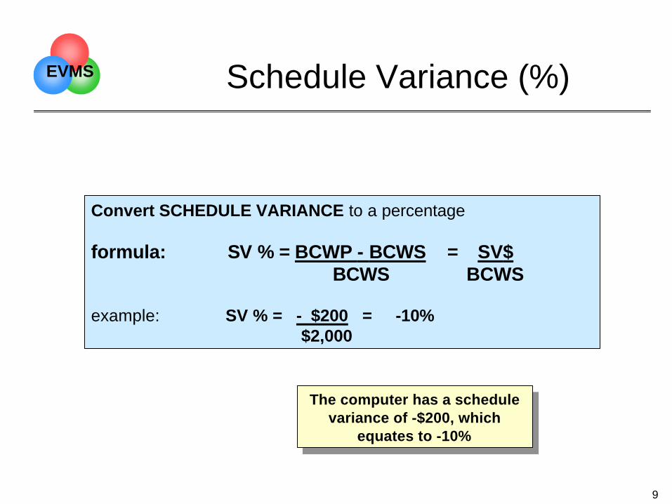
Convert SCHEDULE VARIANCE to a percentage
formula: SV % = BCWP - BCWS = SV$ BCWS BCWS
example: SV % = - $200 = -10% $2,000
The computer has a schedulevariance of -$200, which
equates to -10%
The computer has a schedulevariance of -$200, which
equates to -10%

EVMS
10
Cost Variance ($)
BC WPAC WP
of the work I actually performed,how much did I budget for it to cost?
of the work I actually performed,how much did it actually cost?
COST VARIANCE is the difference between budgeted costand actual cost
formula: CV $ = BCWP - ACWP
example: CV = BCWP - ACWP = $1,800 - $1,900 CV= -$100 (negative = cost overrun)
PE
RF
OR
MA
NC
E B
AS
ED
The computer has a costvariance of $-100
The computer has a costvariance of $-100

EVMS
11
Cost Variance (%)
Convert COST VARIANCE to a percentage:
formula: CV % = BCWP - ACWP = CV $ BCWP BCWP
example: CV % = -$100 = -6% $1,800
The computer has a costvariance of $-100, which
equates to -6%
The computer has a costvariance of $-100, which
equates to -6%

EVMS
12
Price vs. Usage
• In elements with a significant amount of recurring material, contractorshould break CV $ into price vs. usage variance
• problem: I used 10 more widgets than I planned on (58 - 68), andspent $30 more per unit than planned ($300 - $330)
• Price variance = (price difference)*(actual number of units) = -$30 * 68 = -$2,040
• Usage variance = (usage difference)*(original price) = -10 * $300 = -$3,000
• Total cost variance = -$2,040 + - $3,000 = -$5,040
may also performsimilar analysisfor labor (laborrate vs. hours) orfor overhead(rate vs. volume)
may also performsimilar analysisfor labor (laborrate vs. hours) orfor overhead(rate vs. volume)

EVMS
13
Variance at Completion (VAC) ($)
B AC what the total job is supposed to cost
E AC what the total job is expected to cost
VARIANCE AT COMPLETION is the difference between what the totaljob is supposed to cost and what the total job is now expected to cost.
FORMULA: VAC $ = BAC - EAC
Example: VAC $ = $4,000 - $4,500VAC $ = - $500 (negative = projected overrun)
VARIANCE AT COMPLETION is the difference between what the totaljob is supposed to cost and what the total job is now expected to cost.
FORMULA: VAC $ = BAC - EAC
Example: VAC $ = $4,000 - $4,500VAC $ = - $500 (negative = projected overrun)

EVMS
14
Variance at Completion (VAC) (%)
Convert VARIANCE AT COMPLETION to a percentage:
FORMULA: VAC % = BAC - EAC = VAC BAC BAC
Example: VAC % = -$500 = -13% $4,000
Convert VARIANCE AT COMPLETION to a percentage:
FORMULA: VAC % = BAC - EAC = VAC BAC BAC
Example: VAC % = -$500 = -13% $4,000
The computer has a VAC of -$500,which equates to -13%
The computer has a VAC of -$500,which equates to -13%

EVMS
15
Management Reserve (MR)
• If you expect the contractor to use all MR before theend of the contract:
– add MR to BAC when calculating % complete, % spent, % scheduled– add MR to BAC when calculating statistical EACs
– if you add it, be consistent and add to all formulas

EVMS
16
A special note about Indirects
• Typically, indirect loads (overheads, Gen & Admin, COM) make up 40 -50% of a contract’s cost
• To ignore the impact of these rates would be foolhardy• Understand the business assumptions that go into these rates• Have contractor perform rate vs. volume analysis
– example:• Manufacturing overhead total CV: -$3,200K• impact due to actual rate -$ 500K• impact due to volume (loss of commercial business) -$2,700K
• Have DCMC analyst support you with analysis of indirect variances• Assess impact of future rate changes on outyear costs

EVMS
17
1.0
.9
1.1
“GO
OD
”“B
AD
”
1.2
.8
COST PERF INDEX (CPI) = BCWP ACWP
SCHED PERF INDEX (SPI) = BCWP BCWS
COST PERF INDEX (CPI) = BCWP ACWP
SCHED PERF INDEX (SPI) = BCWP BCWS
CPI
SPI
TIME
Performance Indices

EVMS
18
Sample Data Indices
CPI = $1,800 = .95 $1,900
SPI = $1,800 = .90 $2,000

EVMS
19
Where are the significant variances?
BCWS BCWP ACWP SV SV% SPI CV CV% CPI BAC EAC VAC VAC %
Computer 2,000 1,800 1,900 (200) -10% 0.900 (100) -6% 0.947 4,000 4,500 (500) -13%
Radar 230 155 195 (75) -33% 0.674 (40) -26% 0.795 240 195 45 19%
FLIR 550 750 690 200 36% 1.364 60 8% 1.087 1,000 1,500 (500) -50%
Total 2,780 2,705 2,785 (75) -3% 0.973 (80) -3% 0.971 5,240 6,195 (955) -18%
Worst SV ($): computerWorst SV (%): radar
Worst CV ($): computerWorst CV (%): radar
Worst VAC ($): computer, FLIRWorst VAC (%): FLIR
Worst SV ($): computerWorst SV (%): radar
Worst CV ($): computerWorst CV (%): radar
Worst VAC ($): computer, FLIRWorst VAC (%): FLIR

EVMS
20
Sorting on Variances
WBS DESCRIPTION Proj Ofcr %Comp %Spent CPI CV CV CV % VAC VAC
1 3600 PCC Zepka 28.99 34.09 0.850 ↑ -296.2 -17.62 ↔ -187.2
2 3200 COMMUNICATIONS Tideman 34.63 41.03 0.844 ↓ -130.8 -18.49 ↔ -87.0
3 G&A GEN & ADMIN 33.67 36.11 0.932 ↓ -45.2 -7.26 ↔ -36.8
4 2200 SYS ENGINEERING Price 85.04 94.35 0.901 ↓ -26.4 -10.95 ↔ 0.0
5 3800 I & A Troop 35.40 37.08 0.955 ↓ -24.2 -4.75 ↔ -24.8
6 2100 PROJ MANAGEMENT Brown 45.70 48.51 0.942 ↔ -17.4 -6.16 ↔ -3.2
7 2300 FUNC INTEGRA Price 71.62 75.23 0.952 ↓ -17.4 -5.03 ↔ -30.8
8 5200 MANAGEMENT DATA Simmons 84.18 98.10 0.858 ↓ -13.2 -16.54 ↑ -16.0
9 3100 SENSORS Smith 20.87 21.49 0.971 ↓ -10.6 -2.94 ↔ -21.6
10 4000 SPARES Blair 17.87 18.90 0.945 ↑ -7.8 -5.78 ↔ -6.2
11 6200 SYSTEM TEST Hall 60.82 61.66 0.986 ↑ -5.6 -1.38 ↔ -2.0
12 5100 ENG DATA Novak 38.51 52.80 0.729 ↓ -4.6 -37.10 ↔ 0.0
13 MR MGT RESERVE 0.00 0.00 0.0 ↔ 439.2
14 UB UNDIST BUDGET 0.0 0.0
15 COM COST OF MONEY 0.0 0.0
16 3700 DATA DISPLAY Troop 41.13 41.13 1.000 ↔ 0.0 0.00 ↔ 0.0
17 OV OVERHEAD 0.0 0.0
18 6100 TEST FACILITIES Smart 100.00 98.02 1.020 ↔ 2.0 1.98 ↔ 0.0
19 3500 COMP PROGRAMS Pino 46.46 44.66 1.040 ↓ 3.4 3.87 ↔ -1.4
20 6300 PCC TEST Bond 23.13 22.64 1.021 ↓ 4.2 2.10 ↔ 0.0
21 3400 ADPE Zepka 41.89 39.79 1.053 ↓ 12.6 5.02 ↔ 4.6
22 3300 AUX EQUIP Tideman 27.57 24.33 1.133 ↓ 78.2 11.73 ↓ 8.4
sorted by CV $
Analysis software tools (e.g.wInsight or PerformanceAnalyzer) allow you toquickly sort on any columnand spot the significantproblems.
Analysis software tools (e.g.wInsight or PerformanceAnalyzer) allow you toquickly sort on any columnand spot the significantproblems.

EVMS
21
Guidelines
• Start by looking at significant variances ($ and/or %) in CUM data– warning: cum data may mask recent negative variances
• Don’t ignore the significant, positive variances– what is the explanation?
• example:the contractor took earnings for material (BCWP), but the actuals (ACWP) have not yethit. This variance would reverse itself in the next cycle.
• Look at CURRENT period variances– can indicate start of trend, or significant change
• example:element may still have a positive CUM variance, but the current period datashows a significant negative variance
• Variances that are very early (<5% complete) may be misleading• How do I know if it is serious?
– variance greater than +/-10%– sudden trend change– analysis software will flag serious variances for explanation

EVMS
22
Additional screening hints
• BCWR– Budgeted Cost of Work Remaining (BCWR) = BAC - BCWP
• calculated automatically by software
– shows if there is a significant amount of work remaining or not• companion check: percent complete
• Use BCWR and % Complete to screen out elements that are very close tofinishing, are too early to look at, or elements that are too minor
– examples:• example 1: BCWR is $2K, % complete is 55% TOO MINOR• example 2: BCWR is $100K, % complete is 97% TOO CLOSE TO END• example 3: BCWR is $2,400K, % complete is 2% TOO EARLY, BUT WATCH• example 4: BCWR is $2,000K, % complete is 38% LOOK AT VARIANCES
• Focus your analysis efforts on significant elements
EVMS
23
Graph and Analyze Trends

EVMS
24
Tips for Trend Analysis
Cum charts show overall trend...are you getting better,
or worse?
Cum charts show overall trend...are you getting better,
or worse?
Dollars In T
housands
Cumulative Variance MEGA HERZ ELEC & VEN F04695-86-C-0050 RDPR FPI
Element: 3200 Name: COMMUNICATIONS
COSTSCHEDVAC
1992APR MAY JUN JUL AUG SEP OCT NOV DEC
1993JAN
-300.0
-200.0
-100.0
0.0
100.0
1.0 -2.0 3.0
1.0 -18.0 3.0
1.0 -17.0 3.0
-2.0 -28.0 3.0
-13.0 -37.0 -10.0
2.0 -52.0 -10.0
-32.0 -32.0 -10.0
-101.0-207.0 -87.0
-87.4-172.2 -87.0
-130.8-203.2 -87.0
Dollars In T
housands
Current Variance MEGA HERZ ELEC & VEN F04695-86-C-0050 RDPR FPI
Element: 3200 Name: COMMUNICATIONS
COSTSCHED
1992APR MAY JUN JUL AUG SEP OCT NOV DEC
1993JAN
-200.0
-100.0
0.0
100.0
1.0 -2.0
0.0 -16.0
0.0 1.0
-3.0 -11.0
-11.0 -9.0
15.0 -15.0
-34.0 20.0
-69.0-175.0
13.6 34.8
-43.4 -31.0
Current charts show the monthswhere there were significant
performance problems.
Current charts show the monthswhere there were significant
performance problems.

EVMS
25
Total Program VariancesMEGA HERZ ELEC & VEN Cost/Schedule Variance
F04695-86-C-0050 MOH-2 RDPR FPI POP: 01 MAR 1992 - 15 SEP 1993
Percent of D
ollars
COST VARIANCESCHEDULE VARIANCE
1992MAY JUN JUL AUG SEP OCT NOV DEC
1993JAN
-30.0
-20.0
-10.0
0.0
10.0
20.0
30.0
Cost Drivers, Cause
Dollars In MillionsBCWSBCWPACWP
CVSV
0.3 0.2 0.2 0.0 -0.1
0.6 0.5 0.5 -0.0 -0.1
1.0 0.9 0.9 -0.0 -0.1
1.4 1.4 1.5 -0.1 -0.0
2.2 2.2 2.2 0.0 -0.0
2.5 2.7 3.0 -0.3 0.2
4.2 3.8 4.2 -0.5 -0.4
5.6 5.3 5.6 -0.3 -0.3
7.3 6.9 7.3 -0.5 -0.4
At CompletionKTR PO
20.8 20.8
20.8 20.8 20.8 23.0 0.0 -2.2
PMB: 20.4 % COMP: 32.9 MR: 0.4 KTR MR LRE: 0.0 PO MR LRE: 0.0CURRENT FUNDING: 10.0
PO EPC: 24.0PROJ FUNDING: 23.0
AS OF: JAN 93OPR: MR B. TECH
PROGRAM: Mohawk Vehicle
0%
-11%-7%-6%
Analysis:
Both cost andschedule trendshave been negativefor several months,and declined thismonth.
Contractor is 33%complete.
ManagementReserve is .4M (2%of PMB).
Contractor expectsto finish on budget(0% VAC).Program Officeexpects -2.2 VAC,or -11%, andexpects costperformance todecline.

EVMS
26
Trend Chart for Elements
Percent of D
ollars
Cumulative Variance Percent MEGA HERZ ELEC & VEN F04695-86-C-0050 RDPR FPI
Element: 3600 Name: PCC
COSTSCHEDVAC
1992APR MAY JUN JUL AUG SEP OCT NOV DEC
1993JAN
-40.00
-30.00
-20.00
-10.00
0.00
10.00
20.00
0.00 3.57 -5.64
-10.17-24.36 -5.64
-14.40 -4.58 -5.64
-15.91 -0.90 -5.64
-23.08 2.20 -6.36
-12.79 4.38 -6.36
-26.08 14.49 -6.36
-36.45 0.72 -3.37
-23.32 -0.59 -3.37
-17.62 -0.67 -3.23
Analysis:
Cost: this elementexperienced significantcost problems in Aug,Oct, Nov. Shows somerecovery, but still aserious cost variance.Reason why:
Schedule: this elementshowed early scheduleproblems, butrecovered and wassignificantly ahead ofschedule in Oct.Recent performancehas declined and nowslightly behindschedule. Why:
VAC: Contractorrevised (decreased)LRE in Nov and claimsonly -3% at complete.DOESN’T MATCHCOST PERFORMANCE.

EVMS
27
Show performance against technicalperformance
Index of Dollars
CPI and SPI MEGA HERZ ELEC & VEN F04695-86-C-0050 RDPR FPI
Element: 3200 Name: COMMUNICATIONS
CPISPI
1992APR MAY JUN JUL AUG SEP OCT NOV DEC
1993JAN
0.600
0.700
0.800
0.900
1.000
1.100
1.083 0.867
1.038 0.600
1.017 0.776
0.981 0.783
0.920 0.801
1.008 0.823
0.903 0.903
0.769 0.619
0.860 0.758
0.844 0.777
Reliability
0
0.1
0.2
0.3
0.4
0.5
0.6
0.7
0.8
0.9
1
Apr-92
May-92
Jun-92
Jul-92
Aug-92
Sep-92
Oct-92
Nov-92
Dec-92
Jan-93
required
demonstrated
Is there a correlationbetween technicalperformance and earnedvalue performance?
Can poor technicalperformance be used topredict schedule and costproblems?
Use appropriate trend data.What is technical driver thatwould drive performancedata?

EVMS
28
CPI and SPI
Index of Dollars
CPI and SPI MEGA HERZ ELEC & VEN F04695-86-C-0050 RDPR FPI
Element: 1000 Name: MOH-2
CPISPI
1992APR MAY JUN JUL AUG SEP OCT NOV DEC
1993JAN
0.700
0.800
0.900
1.000
1.100
1.200
1.150 1.000
1.051 0.716
0.996 0.912
0.987 0.946
0.927 0.972
1.011 0.993
0.906 1.089
0.891 0.902
0.947 0.948
0.932 0.941

EVMS
29
Snake chart
Dollars In Thousands
Cumulative Element Performance MEGA HERZ ELEC & VEN F04695-86-C-0050 RDPR FPI
Element: 2200 Name: SYS ENGINEERING
BCWS 234.6BCWP 241.0ACWP/ETC 267.4
BAC 283.4LRE 283.4
1992 1993
0.0
100.0
200.0
300.0
400.0 Time N
ow
Com
plete

EVMS
30
EAC Realism
Dollars In M
illions
Estimates at Completion MEGA HERZ ELEC & VEN F04695-86-C-0050 RDPR FPI
Element: 3600 Name: PCC
BACLRECUM CPI
1992APR MAY JUN JUL AUG SEP OCT NOV DEC
1993JAN
5.0
6.0
7.0
8.0
5.1 5.4 5.1
5.1 5.4 5.7
5.1 5.4 5.9
5.1 5.4 6.0
5.1 5.5 6.3
5.1 5.5 5.8
5.1 5.5 6.5
5.5 5.7 7.6
5.5 5.7 6.8
5.8 6.0 6.8
Shows changes in BACand LRE.
Compares budget vs.contractor’s LRE.
Software calculates EACbased on cum CPI.Compare this to theLRE.
Analysis: contractorincreased the budget forthis element twice.Contractor alsoincreased the LREtwice, but NOT ASMUCH as the BAC.Based on pastperformance asreflected in the Cum CPIforecast for EAC, thecontractor’s LRE isUNREALISTIC.

EVMS
31
Keep an eye on Management Reserve
Dollars In M
illions
Cost/Schedule Variance TrendsF04695-86-C-0050 RDPR FPI
Contractor: MEGA HERZ ELEC & VENContract: MOH-2
Program: Mohawk VehicleAS OF: JAN 93
Cost Variance -0.5Schedule Variance -0.4Management Reserve 0.4
10% ThresholdsStart/Comp Dates
Cost Var Est @ CompletionPO -2.2KTR 0.0
1992 1993 -3.0
-2.0
-1.0
0.0
1.0
2.0 Start
Com
plete
Compare MRchanges to costvariances.
CAUTION: MRshould not beapplied to offsetcost variances.
Both MR and UBshould beexplained inFormat 5.

EVMS
32
Comparative Data

EVMS
33
% scheduled = BCWS x 100% = 2,000 = 50% BAC 4,000
% completed = BCWP x 100% = 1,800 = 45% BAC 4,000
Schedule Status
compa
re
I should have completed 50% of the total work.
I only completed 45% of the total work.

EVMS
34
budget status
% spent (original budget) = ACWP x 100% BAC
budget status
% spent (original budget) = ACWP x 100% BAC
compare: % spent vs. % complete
example: 48% spent vs. 45% complete
compare: % spent vs. % complete
example: 48% spent vs. 45% complete
Budget Status

EVMS
35
Compare CV to VAC
Example 1: CV -6%VAC -13%
Example 2: CV -15%VAC -8%
Example 3: CV -12%VAC -12%
I project that performancewill get worse and result in abigger overrun
I project that performancewill get better. I’ll havebetter cost efficiencies inthe future than I do now.
I project that performancewill stay the same
EVMS
36
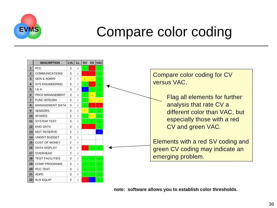
Compare color coding
DESCRIPTION LVL LL SV CV VAC
1 PCC 3 √ ↓ ↑ ↔
2 COMMUNICATIONS 3 √ ↑ ↓ ↔
3 GEN & ADMIN 2 √ ↓ ↓ ↔
4 SYS ENGINEERING 3 √ ↔ ↓ ↔
5 I & A 3 √ ↓ ↓ ↔
6 PROJ MANAGEMENT 3 √ ↑ ↔ ↔
7 FUNC INTEGRA 3 √ ↓ ↓ ↔
8 MANAGEMENT DATA 3 √ ↑ ↓ ↑
9 SENSORS 3 √ ↑ ↓ ↔
10 SPARES 2 √ ↑ ↑ ↔
11 SYSTEM TEST 3 √ ↓ ↑ ↔
12 ENG DATA 3 √ ↓ ↓ ↔
13 MGT RESERVE 2 √ ↔
14 UNDIST BUDGET 2 √
15 COST OF MONEY 2 √
16 DATA DISPLAY 3 √ ↑ ↔ ↔
17 OVERHEAD 2 √
18 TEST FACILITIES 3 √ ↔ ↔ ↔
19 COMP PROGRAMS 3 √ ↔ ↓ ↔
20 PCC TEST 3 √ ↑ ↓ ↔
21 ADPE 3 √ ↓ ↓ ↔
22 AUX EQUIP 3 √ ↓ ↓ ↓
Compare color coding for CVversus VAC.
Flag all elements for furtheranalysis that rate CV adifferent color than VAC, butespecially those with a redCV and green VAC.
Elements with a red SV coding andgreen CV coding may indicate anemerging problem.
note: software allows you to establish color thresholds.

EVMS
37
Analysis of Schedule

EVMS
38
Schedule Analysis
• Early warning: schedule variances are usually an early warning of costvariances to follow
• Schedule variances in EVMS should be seen as indicators andwarnings
• True schedule analysis should be performed on the integrated masterschedule
– Analysis of critical path activity– Work with program office schedule analyst– Performance data and formal schedule should indicate same problems and
risk areas
• Some software allows you to synch the master schedule andperformance data for an integrated assessment

EVMS
39
Converting SV $ to Months
Months ahead or behind = SV $ Average monthly BCWS $
BCWS
BCWP
TIME NOW
MONTHS BEHIND
Either technique can beused to convert SV fromdollars to approximatemonths. Note that this isdependent on average ofwork scheduled and isonly an approximation.
Either technique can beused to convert SV fromdollars to approximatemonths. Note that this isdependent on average ofwork scheduled and isonly an approximation. Draw a parallel
line from BCWPback to intersectBCWS, thendrop down toread off the Xaxis (time).
EVMS
40
Examine written analysis

EVMS
41
• Format 5 variance analysis should address:– separate discussion of CV, SV (current and cum) and VAC– clear description of reason for variance– quantity variances (e.g., price vs. usage)– be specific, not general– corrective action– technical, schedule, and cost impacts– impact to estimate at completion
– should be written by CAM!
Variance Explanations
A big hammer for a big variance!

EVMS
42
• What is a significant variance?– % variance (e.g., >10%)– $ variance (e.g., >$50,000)– critical path element– risk/complexity– impact to other elements– Top 10, Top 20, etc.– contractor defined
Significant Variances

EVMS
43
Work Remaining vs. Risk

EVMS
44
Need to look ahead
Format 5 Narrative Report
Element Code: 25 Project Officer: BUETTGENBACHElement Name: AVIONICS IPT Office Symbol: 25
Schedule Variance:Month: $0K Avionics is essentially on schedule.
Cumulative: ($54K)Cumulative negative variance is due to the following. …………
GCAM, Robert Gemin, 6 Oct. 97
I consider this month's assessment accurate and complete. Looking forward one could expectadditional variances for the following reasons:
SV may increase temporary due to late delivery of... … SV will still appear for the upcomingmonths.
CV will increase in the upcoming month for two reasons. … ..
excerpts from actualanalysis….
Contractor wasincurring relatively smallvariances, but thegovernment managersaw risks ahead
excerpts from actualanalysis….
Contractor wasincurring relatively smallvariances, but thegovernment managersaw risks ahead

EVMS
45
Look Ahead
• Government control account managers (GCAMs) should keep up todate on what the PMB looks like for their element
– “IBR” should be seen as continuous process– Continue the dialogue with contractor counterparts
• Sample:– “I know that we failed the reliability test this month. What impact will
this have on the remaining schedule and budget?”• Don’t wait until the formal report is received
• GCAMs are the technical managers, and understand the nature of thetechnical risks ahead
– Are developing problems in the performance report analyzed and includedin the formal risk plan?
– Are items in the formal risk plan analyzed for cost and schedule impacts?– Are highly probable risk elements included in the EAC?– Is the system engineer evaluating the integration of all elements?
• Program office may wish to perform a formal Integrated RiskAssessment on the program

EVMS
46
Soliciting input from the IPTs

EVMS
47
Analysis within the Program Office
• Assign to technical managers within program offices
– Government Control Account managers (GCAMs)
• Conduct monthly team variance meetings
• Open, honest communication essential– Oral, e-mail, and face-to-face discussions
– Continuing dialogue dramatically improves Format 5
• Early warning analysis– Top level cost and schedule analysis by EVMS and schedule analysts
• analysts should actively seek input from IPTs
– CAM/GCAM analysis at lowest level• analysis should be loaded into network for availability to entire team
• Work closely with DCMC team
• Share results of analysis with contractor

EVMS
48
Program Manager Ownership
• Program managers/IPT leads should be able to access completedata base from their desk
– typical question: “What is this trend telling me?”– PMs go directly to CAMs/GCAMs for details– program managers should focus on significant trends– program managers should receive EVMS training
• Program managers chair variance analysis meetings– not a financial function– should lead dialogue with contractor
• EVMS metrics should be fully integrated into program reviews– internal to company– to government program office
experience shows….
if a program manager shows that he uses EVMSto manage, then the IPTs will follow. It is verydifficult for the IPTs to maintain interest on a longterm basis without this leadership.
experience shows….
if a program manager shows that he uses EVMSto manage, then the IPTs will follow. It is verydifficult for the IPTs to maintain interest on a longterm basis without this leadership.

EVMS
49
Assessing EAC Realism

EVMS
50
• Estimate at Completion (EAC)– defined as actual cost to date + estimated cost of work remaining– contractor develops comprehensive EAC at least annually
• reported by WBS in cost performance report
– should examine on monthly basis– consider the following in EAC generation
• performance to date• impact of approved corrective action plans• known/anticipated downstream problems• best estimate of the cost to complete remaining work
– also called latest revised estimate (LRE), indicated final cost, etc.
What will be the final cost?
ACWP + ETC = EAC

EVMS
51
How can I assess EAC realism?
• Method 1: look at trend chart– compare BAC vs. LRE vs. Cum CPI forecast– portrays size of gap between contractor’s projected performance and past
performance
Dollars In M
illions
Estimates at Completion MEGA HERZ ELEC & VEN F04695-86-C-0050 RDPR FPI
Element: 3600 Name: PCC
BACLRECUM CPI
1992APR MAY JUN JUL AUG SEP OCT NOV DEC
1993JAN
5.0
6.0
7.0
8.0
5.1 5.4 5.1
5.1 5.4 5.7
5.1 5.4 5.9
5.1 5.4 6.0
5.1 5.5 6.3
5.1 5.5 5.8
5.1 5.5 6.5
5.5 5.7 7.6
5.5 5.7 6.8
5.8 6.0 6.8
Standard EAC chart
where’s the miracle?

EVMS
52
• Method 2: compare following data
CPIcum (past cost efficiency)= BCWP
ACWP
TCPI-LRE (projected efficiency needed = Work Remaining = BAC - BCWP to come in at LRE) Estimate Remaining LRE - ACWP
How can I assess EAC Realism?
DESCRIPTION % Compl CV VAC VAC BAC LRE EAC (CPI) CPI TCPI-LRE CPI to LRE
1 SYS ENGINEERING 85.04 ↓ ↔ 0.0 283.4 283.4 314.4 0.901 2.650 -1.749
2 ENG DATA 38.51 ↓ ↔ 0.0 32.2 32.2 44.1 0.729 1.303 -0.573
3 DATA 72.60 ↓ ↔ -16.0 127.0 143.0 151.5 0.838 1.055 -0.216
4 COMMUNICATIONS 34.63 ↓ ↔ -87.0 2,043.0 2,130.0 2,420.8 0.844 1.034 -0.190
5 PCC 28.99 ↑ ↔ -187.2 5,800.6 5,987.8 6,822.4 0.850 1.027 -0.177
6 PROJ MANAGEMENT 62.79 ↓ ↔ -34.0 1,384.6 1,418.6 1,482.1 0.934 1.056 -0.122
EAC Realism Viewrule of thumb
should bewithin 5% ofeach other(.05)

EVMS
53
How can I assess EAC Realism?
Statistical and Independent Forecasts3 PER AVG 6467.8 5777.2 6719.3 7971.4 7171.6 6603.86 PER AVG 6329.8 5800.6 6539.2 7663.2 6883.9 6833.0CUM CPI 6329.8 5800.6 6484.3 7568.9 6840.9 6822.4CUR CPI 7053.4 5024.3 9009.5 9271.7 5687.4 6156.9COST & SCH 5652.6 5376.4 5455.8 6554.9 6302.1 6446.5LINEAR REG 6 383.8 5934.1 6314.3 7339.1 7056.1 7039.5PERF FACTOR 5699.8 5671.9 5761.5 6322.3 6267.5 6508.7USER EAC 0.0 0.0 5455.8 0.0 0.0 6822.4CPI*SPI 6202.1 5581.9 5767.1 7522.7 6872.5 6855.3MICOM EAC 5470.0 5470.0 5815.1 7616.3 6915.7 6866.0
From 6 periodsummaryreport
• Method 3: Compare various statistical forecasts
• for the current month, EACs range from 6,157K to 7,040K• Contractor’s EAC was 5,988K
PAST SIX MONTHS

EVMS
54
Calculate an Independent EAC

EVMS
55
• over 800 military programs show that ......
no program has ever improved performance better than the followingEAC calculation
EAC = BAC CPI
at 15% complete point in program
early stages!no one pays enough attention in the
Survey says…..

EVMS
56
• Variance at Completion vs. Contractor Loss
– Positive VAC:• EAC < BAC underrun contractor gain
– Negative VAC:• EAC > BAC share area contractor partial loss• EAC > ceiling overrun contractor loss (100%)
• Government develops top level EAC for comparison– government will limit progress payments if EAC is greater than ceiling– government needs forecast of fund requirements
• May still have time to change the final outcome
Why do we need accurate EACs?

EVMS
57
• Common EAC Formulae:
EAC = BACCPI
= ACWPcum + Budgeted Cost of Work Remaining CPI3
= ACWPcum + Budgeted Cost of Work Remaining .8(CPI) +.2(SPI)
= ACWPcum + Budgeted Cost of Work Remaining CPI * SPI
One method: statistical formulae

EVMS
58
Other methods of EAC calculation
• “Grass Roots” or formal EAC– detailed build-up from the lowest level detail– hours, rates, bill of material, etc.
• Average of statistical formulae• Show range of EACs (optimistic, most probable,
pessimistic)• Complete schedule risk analysis for remaining
work, estimate work remaining

EVMS
59
Formulate a Plan of Action

EVMS
60
What to do next...
• Have a process for integrated analysis within program office– Include DCMC team– What does the program manager need to see on a regular basis?
• what format? (briefing, memo, or on-line)
– Provide regular training, workshops, etc.
• Make sure that the analysis gets into the right hands– Use flash data to alert the program manager ASAP
• try to get Format 1 or 2 data as soon as possible
– Program management team should be using it to control program– EVMS analysis should be integrated into program management type
reviews– Provide a feedback copy to the contractor and to DCMC

EVMS
61
Mutual Goal: Effective Variance Analysis
• Make it meaningful– avoid routine explanations
• Make it timely– flash data allows for real time discussions
• Make it streamlined– significant variances
• Make it right– work with contractor to get the information we need
• Get the information to the right players
make this a mutual goal
with your contractor

EVMS
62
Forward Look - Focus on the Right Things
Time now
Where we’re goingWhere we’ve been
ETC
BCWRCum SV$
Cum CV$
SPI
CPI
3 month avg
Variance explanation
TCPI-LRE
TCPI-BACProjected variances
Schedule risk
COST HISTORY COST AVOIDANCE
Technical risk

EVMS
63
USE DATA FOR DECISION MAKING
• Behind Schedule - How critical is schedule? - Can I afford to work overtime to recover? - Can I do tasks concurrently? - Are there technical innovations which could speed up the process? - Am I “gold plating” instead of just meeting requirements? - Should I do a schedule risk assessment to project impact to program?
• Over Cost - Can I reschedule tasks? (Timephasing) - Is there a less costly facility I can use? - Are there tasks which can be deleted? - Should the element be added to my risk management profile?

EVMS
64
Special Topics

EVMS
65
Setting up an Early Warning System
• Flash data received ASAP, no written analysis• EVMS and schedule managers review data• Teleconference with DCMC
– evaluate cost and schedule variances– evaluate trends– evaluate against program master schedule
• Prepare top level analysis to program manager andIPT leads
– recommend elements for further analysis
• GCAMs discuss their elements with CAMs– write up own variance analysis
• Don’t wait until you get the report to communicate!

EVMS
66
New Advances in Software Analysis Tools
CAM GCAMPAPER
CPR &SCHEDULE
CPR &SCHEDULE

EVMS
67
Let software tools do the number crunching

EVMS
68
Joint Use of Software Tools
• Trend Analysis - Where Have we Been?– Lowest WBS level or IPT level– color codes, charts
• Projection of future - How Bad Can it Get?– EAC trends– comparison of cost efficiencies
• Focus on problems - What are the significant drivers?– Sort by elements, trends, CAM names– autosync to program schedule
• Format 5 Analysis - What are we doing about it?– Joint analysis, corrective plans, risk mitigation
• Report generator– all formats– can go paperless


