1
Anchoring Inflation Expectations in Unconventional Times:
Micro Evidence for the Euro Area†
Jonas Doverna and Geoff Kenny
b
Abstract: We exploit micro data from professional forecasters to examine the stability of the
distribution of long-term inflation expectations in the euro area following the Great
Recession. Although mean expectations declined somewhat, they remained quite well
anchored to the ECB’s price stability objective. Also, their degree of co-movement with other
variables did not increase noticeably following the Great Recession. In contrast, we document
an increase in long-term inflation uncertainty and a clear shift toward a more negatively
skewed distribution. Such findings are in line with the predictions of theoretical models
emphasizing the impact of the lower bound on policy rates and uncertainty about monetary
transmission. For example, controlling for other factors, announcement dates for non-
standard monetary policy measures are shown to be associated with an increase in long-term
inflation uncertainty.
JEL Classification: E31, E58
Keywords: inflation expectations, credibility, density forecasts, ECB, euro area
______________________________________________________________________________ †
We would like to thank participants at seminars at the ECB, the University of Heidelberg, the Freie Universität Berlin and the
10th International Conference on Computational and Financial Econometrics (CFE, 2016) for helpful comments and suggestions.
The opinions expressed in this paper are those of the authors and do not necessarily reflect the views of the ECB or the
Eurosystem.
a Alfred-Weber-Institute for Economics, Heidelberg University Corresponding author: Bergheimer Straße 58, 69115 Heidelberg,
Germany. Phone: +49-6221-54-2958. Email: [email protected].
b Directorate General Research, European Central Bank, Kaiserstraße 29, D-60311 Frankfurt, Germany.
Phone: +49-69-53058652, Email: [email protected].

2
1 Introduction
A tight anchoring of medium- to long-term inflation expectations around the central bank’s target is
commonly seen as crucial for steering inflation toward this target without suffering substantial economic
costs. However, during recent years, large macroeconomic and financial shocks associated with the Great
Recession and the fact that policy rates reached their Effective Lower Bound (ELB) have led to concerns
about a possible de-anchoring of long-term inflation expectations in the major currency areas. In the case
of the euro area, concerns have focussed on persistently too low inflation or even deflationary risks and an
associated departure of inflation expectations from levels consistent with the ECB’s objective.1 For
example, Draghi (2014) highlights “the risk that a too prolonged period of low inflation becomes
embedded in inflation expectations”. Indeed, recent unconventional monetary policies are often motivated
as addressing such risks.
Much of the recent economic literature attempting to quantify the evidence and risks of such a de-
anchoring - both in the euro area and elsewhere - has focussed only on the mean or first moment of the
distribution of long-term inflation expectations (Demertzis et al., 2009; Gürkaynak et al., 2010; van der
Cruijsen and Demertzis, 2011; Beechey et al., 2011; Demertzis et al., 2012; Dräger and Lamla, 2013;
Mehrotra and Yetman, 2014).2 In this paper, we provide new empirical evidence about the anchoring of
inflation expectations in the euro area considering the full probability distribution surrounding such
expectations.3 Strong theoretical arguments justify the need to study the properties of the full distribution
and not simply focus on mean expectations. In particular, shifts in the variance of this distribution, its
skewness or tail risk can offer additional evidence of any change in agents’ beliefs about future inflation
over the longer term and the factors that may be shaping them. For example, the model of imperfect
credibility in Bodenstein et al. (2012) suggests that achieving the central bank’s inflation objective may
1 Like many other major central banks, the European Central Bank (ECB) is committed to achieve a particular rate of inflation. In
the case of the ECB, this objective is publically announced and defined as an annual increase in the Harmonised Index of
Consumer Prices (HICP) that is “below but close to 2.0%” and it is intended that this is to be achieved over the “medium run”. 2 In particular such studies have focused on possible changes in the mean or in the strength of its co-movement with other
economic variables. The evidence emerging from this literature suggests that long-term inflation expectation were impacted by the
Great Recession. For the US economy, Galati et al. (2011); Nautz and Strohsal, (2014), Autrup and Grothe, (2014), Ciccarelli and
Garcia (2015) all suggests that inflation expectations in the US started to react more strongly to macroeconomic news. Ehrmann
(2015) also reports evidence of a similar increased sensitivity during periods of low inflation. For the euro area, Galati et al.
(2011) identify a structural break in the responsiveness of European inflation expectations to macroeconomic news and Lyziac
and Palovitta (2016) conclude that there are “some signs of de-anchoring”. However, Strohsal and Winkelmann (2015), Autrup
and Grothe (2014) and Speck (2016) have argued that the degree of anchoring did not change around that time. 3 Mehrotra and Yetman (2014) highlight the importance of the full distribution, noting that there are “at least two dimensions to
anchoring … both the level at which expectations are anchored and how tightly expectations are anchored at that level”. Only the
full distribution can speak directly to the latter aspect.

3
become more challenging following a period such as the Great Recession as central bank credibility
becomes more relevant compared to “normal” times (2012). In a similar vein, Beechey et al. (2011)
demonstrate how imperfect information and potential time-variation in the central bank’s objective can be
associated with a sizeable increase in long-term inflation uncertainty, i.e. in the variance of the distribution
for long-term expected inflation.4 However, it is the incidence of the ELB that makes the strongest case for
studying the full distribution. Under the ELB, models of the business cycle exhibit multiple equilibria,
implying that the distribution of long-term inflation expectations may change and attach non-negligible
probabilities to quite distinctive outcomes. For instance, Benhabib et al. (2001) highlight the existence of a
deflationary equilibrium where the ELB is binding and inflation is stuck below target.5 Clearly, the risks
of such bad equilibria will tend to first show up in increased long-term inflation uncertainty or tail risks,
i.e. in the second and fourth moments of the distribution. In addition, models which take account of the
ELB also emphasise that limitations in the central bank’s ability to respond to deflationary shocks lead to
a negatively skewed distribution forlong-term expectations (see for example, Coenen and Warne, 2014;
Hills et al., 2016).
To address our central question, we proceed in three steps. In a first, we test for possible structural change
in the moments of the expected distribution of long-term inflation, exploiting the methods of Bai and
Perron (1998, 2003) to shed light on both the size and timing of possible shifts. This provides direct
evidence about whether or not the Great Recession and its aftermath resulted in any significant changes in
key features of that distribution. In a second step, we exploit the available micro data in a panel setting and
attempt to explain changes in long-term inflation expectations by studying their co-movement with other
macroeconomic variables. Our use of micro data contrasts with most other recent studies mentioned above
which have focussed on average measures of expectations or representative proxies extracted from asset
prices. Although we do not claim a causal interpretation, the analysis of such co-movements sheds light on
possible changes in the degree to which the distribution is anchored. For example, allowing for uncertainty
4 There has been considerable discussion in the wake of the financial crisis about the need for central banks to consider adjusting
upwards their inflation objectives and the euro area has not been immune to these discussions. For example, Ball et al. (2016),
recently make this recommendation as a means to avoid the incidence, severity and costs of hitting the ELB constraint. This
discussion is conceptually distinct from other recommendations which have emphasized increasing short-run inflation
expectations as a demand management device at the ELB. 5 For instance, Benhabib et al. (2001) highlight the existence of a deflationary equilibrium where the ELB is binding and inflation
is stuck below target. More recently, Aruoba and Schorfheide (2015) construct a two-regime stochastic equilibrium in which the
economy may alternate between a “targeted inflation” and a “deflation” regime.5 Busetti et al. (2014) also study the risks of such a
regime in a model with learning and show that it may imply considerable risks of a de-anchoring of long-term inflation
expectations and give rise to a period of sustained low growth in real output.

4
about the central banks objective, and learning on the part of private agents about its ability to hit that
objective, we can expect some positive co-movement between short-term macroeconomic news and long-
term inflation expectations (e.g. as in Beechey et al, 2011). In the spirit of Levin et al. (2004), we also
consider the co-movement of long-term expectations with an ex post measure of central bank performance
to assess whether agents partly update their future long-term expectations by taking into account the rate
of inflation that the central bank has actually delivered. Also, in line with recent discussions about secular
stagnation and deflationary equilibria with simultaneously weak trend growth and excessively low
inflation expectations, e.g. as discussed in Summers (2014) and Eggertson and Mehrotra (2014), we also
examine the co-movement between long-term inflation expectations and corresponding long-term
expectations about the real economy. Using matched individual level expectations, our panel data allows
us study these interrelationships whilst also controlling for other sources of variation that are common to
all forecasters such as observed inflation rates as well as non-standard monetary policy measures in the
wake of the Great Recession. In addition, we provide direct tests of whether these interrelationships have
changed following the Great Recession and during the more recent period when the ELB has been binding
and the ECB has employed non-standard monetary policy. In a third and final step, using a similar set of
appropriately transformed co-variates, we extend the above micro-level analysis to shed light on the
factors which co-move with changes in long-term inflation uncertainty. Again, such an analysis speaks
directly to the question of anchoring because higher uncertainty about long-term inflation prospects
implies that the distribution is less tightly anchored even if overall mean expectations remain unchanged.
The layout of the remainder of the paper is as follows. In Section 2, we briefly describe our dataset and the
manner in which we estimate key moments of the probability distribution surrounding the long-term
inflation expectations. Section 3 presents the evidence for breaks in these moments. In Section 4, we turn
to the analysis of the variables which co-move with changes in long-term mean expectations and
uncertainty and analyse whether the strength of this co-movement has changed following the Great
Recession. Section 5 concludes by discussing the economic significance of our findings and their
implications for monetary policy.

5
2 Data and Estimation of Density Moments
We base our analysis on the densities of individual forecasters as provided by the ECB’s SPF which has
been conducted and published by the ECB at a quarterly frequency since the beginning of 1999. Since we
are interested in long-term inflation expectations, we primarily focus on those forecasts that have a
forecast horizon of roughly five years (i.e. twenty quarters or ℎ = 20). Our sample period ranges from
1999Q1 to 2017Q1.6 Reflecting its survey origins, the SPF data set is heavily unbalanced because
forecasters leave the panel or enter later and because they are not required to report their forecasts in every
survey round. The number of individual respondents therefore varies from one quarter to the next. We
focus on the analysis of this unbalanced panel and, in particular, do not attempt to interpolate any missing
observations. The number of respondents providing the histograms depicting the probabilities they assign
to a range of future outcomes averages 39.1 in our sample. Although this is slightly lower than the number
of respondents who report point forecasts for inflation (44.6 on average), it nonetheless provides a rich
cross-sectional basis for econometric analysis. Moreover, when considering co-movement with other
variables, we are able to match the estimated moments for inflation at the individual level with
corresponding individual moments estimated from equivalent histograms for GDP growth and the
unemployment rate. Appendix I provides further information on the SPF and other data sources used in
the empirical analysis.
Before attempting to study the properties of the full distribution for long-term expected inflation, it is
necessary to estimate the key moments summarizing the distribution’s location, spread, symmetry, and tail
risks. The density forecasts are provided as histograms for which every forecaster reports probability
forecasts that reflect their assessment of the likelihood that future inflation will fall within certain
intervals. Formally, denote with ��,�|��
the probability that forecaster i ( = 1,… ,�) in survey period t
attaches to the event that the inflation rate in period t+h falls into a particular interval j (� = 1,… , �).7 To
compute mean long-term expectations, the corresponding inflation uncertainty, and higher moments of the
density forecasts, we adopt the most common approach which is non-parametric and assumes that all the
6 Note that during the first two years of the SPF long-term forecasts were only surveyed on an annual basis in 1999Q1 and
2000Q1. We make use of these observations whenever possible. However, we have to drop them from our econometric estimation
whenever we relate long-term expectations to lagged information from the SPF. 7 Note that K changes over time as the survey design was changed at several points in time. We tackle this issue by assigning a
probability of 0 to intervals that were not included in a particular survey round.

6
probability mass in a particular interval j is compressed at the midpoint of this interval, which we denote
by ��. The first four moments are then computed recursively and are given by
(2.1) Mean: ��,�|� = ∑ ��,�|���
��� ��
(2.2) Variance: ��,�|�� = ∑ ��,�|�
����� ��� − ��,�|��
�
(2.3) Skewness: ��,�|� = ∑ ��,�|���
��� ��� − ��,�|���/��,�|�
�
(2.4) (Excess) kurtosis: !�,�|� = ∑ ��,�|���
��� ��� − ��,�|��"/��,�|�
" − 3
For each moment $ = {�, ��, �, !}, we construct the cross-sectional average as $'�|� = 1/
��|� ∑ $�,�|�()*+|)��� , where ��|� denotes the number of density forecasts with a forecast horizon of ℎ
quarters available at time ,. As highlighted in Engelberg et al. (2009), it must be acknowledged that our
moment estimates are subject to measurement error reflecting the random variation in response rates,
panel composition and the assumptions we make regarding the allocation of probability mass to the mid-
points of the surveyed intervals. However, alternative approaches, such as the fitting of a flexible
parametric distribution as in Engelberg et al. (2019), yield very similar estimates.
Note that an estimate of ��,�|� is also available directly from the reported point forecasts that are
collected in the SPF. However, by relying on the estimate based on the histograms we can ensure
consistency of our results across the different moments. A focus on mean expectations from equation (2.1)
is also justified because it draws on all the probabilities collected from respondents. As such, it may
contain more information than the long-term point forecasts that are also collected in each survey round.8
Figure 1 plots the mean estimated according to equation (2.1) together with two other measure of central
tendency taken from the survey. The first is the mode computed as the mid-point of the interval which is
assigned the maximum probability, again averaged across the responding forecasters in a given round. The
second alternative measure is simply the average point forecast. Overall, one observes a very clear co-
movement and similarity between these three measures of central tendency. In particular, the average
point forecast and the estimated mode are very closely related, suggesting that when they give their point
8 García and Manzanares (2007) provide evidence that the density forecasts from the SPF are more reliable than the point
forecasts.

7
forecasts survey respondents may be giving a modal prediction. However, in the period since the financial
crisis mean expectations dropped slightly below both the estimated average mode and the reported point
forecasts. Given this divergent pattern we also include the estimated mode of the probability distributions
in our empirical analysis of potential shifts in the distribution’s location.
[Insert Figure 1 about here]
3 Identifying Breaks in the Distribution of Long-term Inflation Expectations
In this section we report our empirical analysis of possible structural breaks in the distribution of long-
term inflation expectations. We first discuss the econometric specification used to estimate possible breaks
in the distribution before reporting the main findings.
3.1 Testing for Breaks in Density Moments
A powerful set of conditions for inflation expectations to be fully anchored is that their distribution is
stable around the central bank’s inflation target. To examine this, we test for evidence of any breaks in the
first four moments estimated above. We employ the method of Bai and Perron (1998, 2003), who consider
the linear regression model with a finite number of possible regimes defined by unknown breaks in the
model parameters. Their method yields estimates of the unknown regression coefficients associated with
each regime together with estimates of the unknown break points. To select the number of significant
breaks and to date their occurrence, we apply these methods by regressing a given moment on its first lag
and an intercept term. The inclusion of the latter is intended to account for the strong persistence in such
long-horizon moments when estimated at a quarterly frequency and which would otherwise cause
substantial residual autocorrelation in our regressions.9 Formally, the considered model is
(3.5) $'�|� = -.,/ + 1.,/$'�2�|�2� + 3�|�.
where -.,/ and 1.,/ are regime-specific parameters (with 4 = 1,… , 5) and 3�|�. is an iid error term. The
mean of each moment $ = {�, ��, �, !} conditional on being in specific structural regime can be
9 According to the Ljung-Box test, we can reject the null hypothesis of residual autocorrelation at the five percent level for both
the specification without structural breaks and the one with breaks for all moments with one exception: in the case of inflation
uncertainty, the large structural break causes mild negative autocorrelation in the residuals of the specification that does not allow
for this break.

8
computed as -.,//(1 − 1.,/). For the case of mean long-term expectations ($ = �), for instance, this
yields an estimate of the average expected rate of long-term inflation in a given regime. Under the
assumption that forecasters believe that, in general, the central bank is able to achieve its inflation target in
the absence of further shocks such an estimate provides a regime-specific measure of the perceived
inflation objective. In the absence of any structural breaks, we have -8,/ = -8 and 18,/ = 18 which
implies that the long-term expectation for inflation is constant. In a similar way, for each of the three
higher order moments, -.,//(1 − 1.,/) is an estimate for the average perceived future variance, skewness
and tail risk embodied in the distribution in any given regime. Breaks of these higher order moments may
additionally signal changes in the degree to which the distribution of long-term inflation expectations is
anchored.
In implementing the Bai-Perron procedure it is necessary to specify a minimum required distance between
any two potential break dates. We set this minimum distance between breaks at a relatively conservative
level of eight quarters in order to avoid overfitting and possibly finding an implausibly large number of
spurious breaks for each moment. We determine the number of structural breaks by looking at a modified
Schwarz criterion (LWZ) which is suggested for the case of models that include a lagged dependent
variable and the sequential SupF-test which is the overall preferred test according to Bai and Perron
(2003).10
3.2 Breaks in the Mean
Using the approach outlined in the previous section, we analyse whether there have been any substantial
regime changes in the distribution of long-term inflation expectations in the euro area. Figure 2 shows the
evolution of the modal expectation discussed above together with the first four moments given by
equations (2.1) to (2.4). In each panel, the regime-specific estimates -9.,//(1 − 1:.,/) are also plotted (as
identified by the LWZ statistic). The break-point analysis of density moments is further detailed in
Table 1. In particular, we report a list of the estimated break dates and the corresponding F-statistics
indicating the significance of each break as well as complementary results based on the sequential test.
10 The sequential test is based on the idea of sequentially testing the null hypothesis of ; breaks versus ; + 1 breaks until the null
hypothesis can no longer be rejected. In particular, given a set of ; break points, Bai and Perron (1998) suggest to apply ; + 1 tests
of the null hypothesis of no structural break against the alternative hypothesis of a single structural break to the ; + 1 segments of
a time series defined by the ; breaks.

9
[Insert Figure 2 about here]
[Insert Table 1 about here]
For the mean expectations, we find one significant breaks in 2013Q2 according to the LWZ statistic
reported in Table 1. The break is downward and occurs in the wake of the Great Recession and euro area
sovereign debt crisis. Although quantitatively modest it is noticeable with the regime-specific mean falling
to 1.69% from 1.90% prior to the break. The drop in mean expectations is found to be statistically
significant given the low overall volatility of the time series. The case for a significant downward shift of
long-term inflation expectations is weakened, however, by two additional findings. First, the sequential
SupF-test does not identify any breaks in the dynamics of mean expectations and as a result the estimate
for the average over the full sample is constant at 1.83. Second, both tests do not identify any breaks in the
case of modal expectations which average 1.89% over the full sample. A finding of a downward break in
the mean combined with a stable modal value is consistent with a shift toward a more negatively skewed
distribution and we examine this hypothesis directly below by applying the same test to the estimated third
moment.
Overall, our results for mean expectations provide at most only weak evidence for a quantitatively modest
decline in long-term inflation expectations toward the end of our sample. Mean inflation expectations also
remain in a range that can be considered consistent with price stability as defined by the ECB’s price
stability objective of “below but close to 2.0%”. Hence, our analysis provides no grounds to think that the
central tendency of euro area long-term inflation expectations became unanchored. This finding is in line
with other recent studies that use market-based inflation expectations, as, for instance, Strohsal and
Winkelmann (2015), Autrup and Grothe (2014) and Speck (2016).
3.3 Breaks in the Variance
Figure 2 and Table 1 report equivalent results for higher moments. In the case of long-term inflation
uncertainty, both tests identify a break in 2009Q2 that is associated with an increase in uncertainty about
long-term inflation. In relative terms, this shift is quantitatively more noticeable compared with the shift in
mean expectations. After the break, i.e. in the immediate wake of the Great Recession, average uncertainty
about the long-term inflation at 0.66 percentage points (pp) had increased by about 25% compared with its

10
level in the pre-crisis regime (0.53 pp). Following this increase, long-term inflation uncertainty has been
quite stable at the new level and has shown no tendency to decline. This pronounced and persistent
increase in the variance of the distribution signals that forecasters perceive the long-term inflation outlook
to be more uncertain now than before the Great Recession.11
As a result, the distribution has become less
concentrated around levels that are consistent with the definition of price stability. The increase correlates
well with an increase of the historical variance of annual inflation rates in the euro area when computed
recursively based on an expanding sample starting in 1997; the latter increases from about 0.2 in 2007 to a
little below 0.6 in 2014. Thus, it seems as if forecasters anticipate that the increase in inflation volatility
which emerged after the Great Recession will be highly persistent – or even permanent – rather than being
relevant only to recent years or the short-term outlook for inflation.
Overall, the identified upward shift in the variance could be taken to imply that the degree to which long-
term inflation expectations are anchored has diminished. The shift in the variance is also consistent with
macroeconomic theories highlighting the implications of uncertainty surrounding the central bank’s
objective (Beechey et al., 2011) and, in particular, the potential effects of the lower bound on nominal
interest rates (Benhabib et al., 2001). However, the higher variance is also consistent with the view that
forecasters believe it may take longer for the central bank to achieve its price stability objective, e.g. as a
result of more persistent and volatile shocks in the future or a perceived change in the transmission of
monetary policy. It does not necessarily imply that they have reduced their belief in the ECB’s ability to
ultimately achieve that objective over a longer horizon than the five years to which the survey data relate.
Nonetheless, our findings highlight an important challenge for monetary policy and its communication;
namely to limit any further the rise in the uncertainty surrounding long-term inflation prospects.
3.4 Breaks in Symmetry and Tail Risk
Figure 2 and Table 1 also report the results of the break analysis for the skewness and tail risk in the
distribution of long-term expected inflation in the euro area. The time path of the average skewness
provides insight on possible changes in the overall symmetry of the distribution and may thus signal
concerns among forecasters about long-term inflation risks either to the upside or the downside. Figure 2
11 It is noteworthy that the upward adjustment came quite soon after the Great Recession and the sovereign debt crisis was not
associated with any further rise in long-term inflation uncertainty.

11
suggests that, since 2010Q1, the forecast densities are negatively skewed, on average, whereas prior to this
date they were broadly symmetric. This means that since the Great Recession forecasters have been more
concerned about deviations in the direction of lower inflation and less concerned about deviations in the
direction of higher inflation. This finding of a negatively skewed distribution is in line with our previous
result of a possible downward break in mean expectations with a higher and more stable mode. It is also
precisely what is predicted by macroeconomic models which incorporate a lower bound constraint on
nominal interest rates (e.g., Coenen and Warne, 2014; Hills et al., 2016). Interestingly, according to the
LWZ test results reported in Table 1, the break in skewness occurred relatively soon after the Great
Recession and prior to the break in mean expectations. The tendency toward a negatively skewed
distribution has also been highly persistent and has lasted up to the end of our sample in 2017Q1. At the
same time, these results have to be taken with some caution because the alternative SupF-test identifies no
break in skewness. For the kurtosis, we also find no significant break. However, the long-term inflation
density is platykurtic, which means that forecasters believe that, relative to a normal distribution, less of
the inflation uncertainty is associated with infrequent tail events. Overall, therefore, the survey data tends
to give relatively small weight to tail risks for inflation.12
Together with the increased variance, the above distributional changes that we have identified imply a
marked rise in the probability of very low future inflation rates at long-horizons. Figure 3 provides a
summary of how shape, symmetry and tail risk implicit in the survey indicators have changed over time.
The left plot shows how much probability weight the forecasters attributed, on average, to long-term
outcomes of inflation below 0.0%, below 1.0%, and above 3.0%. It is clear that while the risk of a
sustained outright deflation with a falling price level is still perceived as being very low, the perceived
probability that inflation will be below 1.0% has climbed steadily from very low levels prior to 2007 to
around 10.0% in the period 2009 to 2012 and to roughly 12.5% recently. In contrast, the probability that
inflation will be above 3.0% has recently declined to its pre 2007 level after an intermezzo of slightly
higher values over the period 2008 to 2013. The right plot shows the inflation-at-risk measure that is
proposed by Andrade et al. (2012). For each wave of the survey, this indicates the 5th and 95
th percentiles
12 This is a well know finding in the literature exploiting such data. It is a direct consequence of the fact that many participants in
the SPF attach positive probability weights to only a very limit number of the provided bins (see Kenny et al., 2015).

12
of the reported long-term density forecasts for inflation.13
Again, while the 95th percentile (that is
informative about the upper tail of the distribution) is currently more or less unchanged compared to its
value in 2007, the 5th percentile (that is informative about the lower tail of the distribution) declined from
above 1% in 2007 to 0.7% in the first quarter of 2017.14
Overall, forecasters see more risks on the
downside which corresponds to our finding of a structural break in the skewness of long-term forecast
densities after 2010.
[Insert Figure 3 about here]
4 Co-movement of Distributional Moments with other Variables
The previous section provided evidence that the distribution of long-term inflation expectations in the euro
area may have changed in the period since the Great Recession. In particular, our analysis shows that it
experienced a modest downward shift in its mean, a more sizeable and significant increase in its
dispersion, and a persistent negative skewness. As discussed in the introduction, a second way to shed
light on how well-anchored long-term inflation expectations are is to examine the strength of their co-
movement with other economic variables. In a perfect world with no uncertainty about monetary policy
effectiveness, we might expect to observe no correlation between moments of the distribution of
expectations and other macroeconomic developments. However, in a world with uncertainty and learning
on the part of private agents, some co-movement even with short-term macroeconomic developments at
business cycle frequencies can be expected. In such circumstances, an increased sensitivity of long-term
inflation expectations to such factors would be indicative of a change in the degree to which expectations
are anchored.
In this section, we examine the co-movement between the first two moments of the distribution of
expected long-term inflation with other economic variables.15
In particular, we exploit the individual
expectations in a panel setting to address the following questions: Are there factors that co-move strongly
with long-term inflation expectations and uncertainty? Did the role of such factors change after 2007, the
13 To extract these percentiles, we follow Engelberg et al. (2009) and use the approximation of the true density forecasts derived
by fitting the generalized Beta distribution. Hence, results are not directly comparable to other results presented in this paper. The
5th and 95th percentiles are then computed as the average across all individual forecaster. 14 This means that forecasters, on average, expect inflation five years ahead to be below 0.7% with a probability of 5%. 15 We focus on the first two moments because these are the ones for which we can identify a set of appropriate co-variates.
However, given the results of the break test analysis in Section 3 above, the examination of co-movement with the skewness of
the distribution of long-term inflation expectations represents an important area for future empirical research.
13
year in which the financial crisis began to unfold? Can we identify any coincidences between recent
monetary policy events – such as the hitting of the ELB on nominal interest rates or the introduction of
non-standard monetary policies – and changes in the first two moments of the distribution? We first
present the results for the mean and then turn to the analysis of the variance.
4.1 Long-term Mean Inflation Expectations
To examine the co-movement between mean expectations and other macroeconomic developments, we
consider the following set of variables: First we consider, forecaster specific short- and medium-term
inflation expectations at horizons of 1 and 2-years ahead (<=�>�(1?)@� and <=�>�(2?)@�). In addition, we
look at the reaction of long-term expectations to past short- and medium-term forecast errors for inflation,
again at the individual level (π − =�>π(1y)@C2" and π − =�>π(2y)@C2D). To capture perceived structural
changes linked to possible concerns about secular stagnation and deflationary equilibria, we include the
change in long-term expectations for GDP growth (d=�>GDP(5y)@�) and the unemployment rate
(d=�>U(5y)@C) from the SPF. In the spirit of Levin et al. (2004) who show that long-term inflation
expectations in the US and the euro area were highly correlated with a slow moving average of inflation
over the period 1994 to 2003, we also consider an inflation “performance gap” as the difference between
recent long-term expectations and a (five-year) moving average of past inflation (MA(π)C2� −
=�>π(5y)@C2�). In addition to these individual-specific variables, we also consider the possible co-
movement with factors that are common across forecasters, such as shocks to the inflation process itself as
reflected in the recently observed change in the inflation rate (<��2�) and in oil prices (<M ;�2�).16
Also,
we consider the change in the volume of the ECB’s balance sheet (dCBBSC2�) as a monetary policy
indicator that is associated with recent quantitative easing, with the expectation that an expansion of the
balance sheet might potentially lead agents to change their expectation of the long-term inflation rate
upwards. To control for important monetary policy changes, we additionally include a dummy variable for
quarters following the announcement of important non-standard monetary policies (QRS�)17
and a dummy
capturing the hitting of the effective lower bound (=TU�).18
16 Beechey et al. (2011) and Badel and McGillicuddy (2015) document a substantial co-movement of long-term US inflation
expectations with oil prices. 17 The events are: the introduction of enhanced credit support on May 7, 2009; the introduction of the Security Market Program
(SMP) on May 10, 2010; the introduction of the Outright Monetary Transaction (OMT) program on August 2, 2012; the

14
We use an unbalanced pooled panel regression with fixed effects to look at the co-movement discussed
above and to test whether the correlation structure has changed since the Great Recession. Let
∆��,��W|� = ��,��W|� − ��,�2��W|�2� denote the change in the long-term inflation expectation of an
individual forecaster. We regress this change on forecaster-specific fixed effects and the set of proposed
co-variates. Collecting the forecaster specific variables in a vector X�,� and the common co-variates in Y�,
the linear panel regression is given by
(4.1) ∆��,��W|� = -� +QRS�1Z[\ + =TU�1]^_ + X�,�1̀ + Y�1a + 3�,�
where 3�,�is an error term that we allow to exhibit both spatial and temporal correlation (Driscoll and
Kraay 1998).19
The parameter vectors 1Z[\, 1]^_, 1` and 1a measure the extent to which long-term
expectations co-move with the other variables. For perfectly anchored inflation expectations, we would
expect the effect of the two dummy variables to be insignificant and also both 1` = 0 and 1a = 0.
Before proceeding to the results of this full panel analysis, it is of interest to examine the simple bi-variate
co-movement in our dataset. Table 2 reports some basic summary statistics depicting the pair-wise
correlations between mean expectations and the above-proposed regressors. Because we are dealing with
panel data, we can distinguish between the total correlation which is based on the pooled data set, the
between-forecaster correlation which is the correlation between the sample averages for individual
forecasters, and the within correlation which we compute as the mean of the correlations obtained for each
forecaster individually. From an economic point of view, the latter is of greatest interest because
expectations are formed at the individual level. We show the mean, minimum, 10th percentile, 90
th
percentile and maximum value for those forecasters in our sample with at least 8 observations. Total and
between correlations that are statistically significant are marked with *. The last two columns of Table 2
indicate which fraction of forecaster-specific correlations is significantly different from zero or
significantly different from zero and positive (both as a % of the total number of forecasters for which we
can compute the pair-wise correlations).
introduction of forward guidance on July 4, 2013; and the introduction of the enhanced asset purchase program (APP) on January
22, 2015. 18 This dummy takes a value of one for the two survey rounds that follow the dates when the ELB was reached for the ECB
deposit rate (on July 11, 2012) and for the main financing rate (on June 5, 2014), respectively, and zero otherwise. 19 Given that forecasters form their predictions simultaneously and that professional forecasts are usually found to be subject to
information rigidities (Coibion and Gorodnichenko, 2012; Dovern et al., 2015), which cause forecast revisions to be
autocorrelated, both features are important. Ignoring them and assuming independently distributed error terms is likely to results
in an underestimation of the true long-term covariance.

15
From the ten variables that we consider, nine have a significant total correlation with the change in long-
term inflation expectations, suggesting that long-term inflation expectations are not perfectly anchored but
indeed get revised frequently in response to shocks. These correlations range from 0.05 (in absolute
values) to 0.31 (see Table 2). More interestingly, however, are the within correlations that provide a more
nuanced picture. While the mean correlation is higher (in absolute values) in all cases than the
corresponding total correlation, for most variables a relatively small fraction of the underlying correlations
are significantly different from zero. For example, less than 10% are so in the case of both lagged forecast
errors, the change in inflation, the change in oil prices, and the change in the volume of the ECB’ balance
sheet. We obtain the largest fraction of significant correlations in the case of short- and medium-term
inflation expectations (17.3% and 26.9%, respectively) and the central bank performance index (26.9%).
Looking at the last column of Table 2 it is evident that the significant co-movements usually have the
expected sign. For example, for all of the 26.9% of forecasters with a significant co-movement with the
inflation performance gap, the correlation implies that a deviation of actual inflation above the central
bank’s target is associated with an upward revision in long-term inflation expectations. One exception is
the co-movement with the change in long-term growth expectations which is negative in almost one third
of the significant cases. In terms of heterogeneity across forecasters we see a wide range of estimates,
ranging from substantially negative to very large positive correlations in all but one case.
[Insert Table 2 about here]
Table 3 lists the results of estimations of equation (4.1). Specification (1) reports full sample results. To
avoid a potential problem of multicollinearity between the change in the inflation rate and the change in
oil prices, we drop the latter variable from the panel estimation in line with the idea that the impact of oil
prices can be adequately captured through its effects on headline inflation. Specification (2) allows all
parameters in the equation (except for the fixed effects) to break after 2007Q3, which we chose because it
represents the start of the Great Recession and the launch of monetary policy measures aimed at mitigating
turbulences in financial markets. Note that results in the second and third column refer to one regression
and are listed in two columns only for expositional purposes.
[Insert Table 3 about here]

16
Looking first at the full sample results, we observe that only few of the marginal correlations remain
significantly different from zero. In particular, those are the correlations with the change in 2-year
inflation expectations and with the inflation performance gap. For example, long-term inflation
expectations are revised by roughly 0.17 pp, on average, when two-year-ahead expectations move by 1 pp.
Thus, the co-movement is relatively strong, supporting evidence from US household expectations
provided by Dräger and Lambla (2013). According to the estimated parameter values, a 1.0 pp deviation
of the past inflation trend above the announced price stability objective is associated with an upward
revision in long-term inflation expectations of just below 0.15 pp. This highlights the importance of
actually hitting the inflation target in the medium-run if long-term inflation expectations are to be
stabilised. The observed co-movement is in line with macroeconomic theories which allow for uncertainty
about the central bank objective. For example, if private agents are uncertain about the true inflation
objective held by the central bank they may adjust their long-term inflation expectations upward in
response to past inflation trends (see, for example, Beechey et al, 2011).
In our panel regression results, we also find some quantitatively less important but significant co-
movement with the change in actual inflation.20
The only other significant parameter estimate corresponds
to the change in the size of the ECB’s balance sheet. The negative sign appears counterintuitive at first and
demonstrates that the estimates should not be interpreted causally. In this particular case, a valid
interpretation is not that expanding the balance sheet causes inflation expectations to decline. Instead
reverse causality is the most plausible explanations, and also, possible omitted variable bias. For example,
a plausible explanation of the negative co-movement is that the ECB anticipated a decline in expectations
and responded with expansionary measures that were associated with an expansion of the balance sheet.
On the other hand, both the ECB and the forecasters included in our panel could simply respond to
macroeconomic news that we do not capture with our variable selection. Turning to the additional
monetary policy dummies, we find no evidence for any impacts on our measure of mean long-term
expectations. This implies that the hitting of the ELB or the announcement of non-standard measures were
not immediately followed by a change in inflation expectations. This result is not so surprising given the
other controls and co-movement that we have captured in the regressions. For example, it is entirely
20 This is in contrast to Beechey et al. (2011) who find a response of long-term inflation expectations to inflation news for the US
but not for the euro area. However, the sample period used in this study did not cover the period associated with the aftermath of
the Great Recession.

17
plausible that the effects of the ELB and the announcement of non-standard measures are captured via the
co-movement with 2-year-ahead expectations. The result may also be due to the low frequency of the SPF
data which makes it harder to connect changes in expectations to specific events. Based on data of higher
frequency around such announcements, Karadi (2017) shows that non-standard measures by the ECB may
have helped to prevent long-term inflation expectations from becoming unanchored after 2013.
The second set of estimates suggests that the estimated co-movement did not change much after the Great
Recession. An F-test of the joint hypothesis that none of the model’s coefficients exhibits a structural
break in 2007 does not reject this hypothesis. Testing each of the coefficients separately reveals that the
coefficient change is significantly different from zero only in the case of the change in the ECB’s balance
sheet.21
The pre-2007 estimate is strongly negative and highly significant, suggesting that this period also
drives the full-sample results.22
In contrast, the estimate for the sample since 2007Q4 is much smaller and
only significant at the 10% level. Another interesting effect in the post crisis sample is a negative
correlation of mean inflation expectations with changes in long-term unemployment expectations that are
not already captured by the other co-variates. Such negative co-movement is consistent with concerns
about secular stagnation, with simultaneously higher expectations for long-term unemployment being
associated with weak overall inflation expectations. The impact is, however, quantitatively small
compared with the co-movement with other variables.
In summary, the panel regressions suggest that the process governing the mean of the distribution of long-
term inflation expectations is far away from a simple stylized case where the inflation objective is a
universal constant and where there is “blind faith” in the ability of the central bank to achieve this
objective. Instead, this process is more in line with theories emphasising uncertainty about the monetary
policy transmission mechanism in which agents update their beliefs about long-term inflation in response
to relevant shocks. However, there is no evidence of a substantially higher sensitivity to the main co-
variates following the Great Recession. This result is also in line with previous results in Section 3, where
we identified at most only weak evidence that mean inflation expectations had declined following the
21 These results are clearly a reflection of the major structural break in the balance sheet data after the onset of the financial crisis;
changes in the balance sheet size were very small and regular before 2007 and larger and also more volatile afterwards. 22 Given that changes in the size of the balance sheet during this period were largely determined endogenously by the demand for
currency and the minimum reserve requirements, the observed correlation should not be interpreted as a genuine “policy effect”.

18
Great Recession. At the same time, the co-movement that we have identified highlights that the anchoring
of the mean of this distribution can in no way be taken for granted.
4.2 Long-term Inflation Uncertainty
We now turn to the co-movement of long-term inflation uncertainty with other variables. We follow the
same analytic approach but adjust the set of variables that we consider to correspond to the new variable
of interest. In particular, we now look into the co-movement with the change in short- and medium-term
inflation uncertainty (instead of expectations), and with the absolute value of lagged forecast errors and
the difference between recently held long-term expectations and the five year moving average of past
inflation. We also consider the co-movement with long-term uncertainty about growth and the
unemployment rate (instead of expectations), and with the absolute value of changes in the inflation rate,
oil prices and the size of the ECB balance sheet size. As with mean expectations, we use a panel
regression to analyse co-movements of long-term inflation uncertainty to the considered variables jointly.
Denoting by ��,��W|�� = ��,��W|�
� − ��,�2��W|�2�� the change in the long-term inflation uncertainty of an
individual forecaster, we use - analogously to equation (4.1) - the following panel specification:
(4.2) ��,��W|�� = -�
∗ +QRS�1Z[\∗ + =TU�1]^_
∗ + X�,�∗ 1̀ ∗ + Y�∗1a∗ + 3�,�
∗
where X�,�∗ denotes the set of appropriately transformed forecaster specific covariates and Y�∗ the set of co-
variates that are common across forecasters. As a precursor to the results of the main panel regressions, we
again present the between and within forecaster pairwise correlations with the 10 variables considered
(Table 4). There is evidence of substantial and significant co-movement between long-term inflation
uncertainty and short- and medium-term inflation uncertainty (total correlation of 0.39 and 0.52
respectively), long-term uncertainty about growth (0.53), and long-term uncertainty about the
unemployment rate (0.44). Thus, uncertainty about the inflation rate in the long-term co-moves primarily
with uncertainty about the nearer-term inflation outlook and with uncertainty relating to real prospects for
growth and unemployment. Also the corresponding within forecaster co-movement is high for each of
these four variables. Heterogeneity across forecasters is again large, but roughly one quarter to one third of
individual forecasts exhibit correlations that are significantly different from zero and, of these, the
overwhelming number of cases have the expected positive sign.

19
[Insert Table 4 about here]
Table 5 reports the results of estimations of equation (4.2). Overall and compared to mean expectations, a
higher share of variation of long-term inflation uncertainty can be explained by movements in the
covariates considered in our study (R2 of 0.39 for the full sample). The main findings are as follows: First,
long-term inflation uncertainty co-moves strongly with inflation uncertainty at a two-year horizon.
Second, absolute changes in the current inflation rate are positively correlated with long-term inflation
uncertainty. Thirdly, we find a strong and highly significant positive co-movement with the perceived
uncertainty about long-term growth rates and the long-term unemployment outlook.
The panel regressions for uncertainty also reveal some important co-movement with the indicators linked
to monetary policy. In the full specification, active monetary policy – associated with large changes in the
volume of the assets held by the ECB – tends to be associated with, on average, a reduction in long-term
inflation uncertainty. This result suggests that monetary policy has, in absolute terms, contributed to
reducing inflation uncertainty over our sample. However, when one considers the persistent rise in long-
term uncertainty highlighted in Section 3, monetary policy was not able to fully insulate long-term
inflation uncertainty from the other factors discussed above. Looking at the coefficients corresponding to
the monetary policy dummies, we find that the announcement dates for non-standard measures were
generally associated with an increase in inflation uncertainty although this effect is quantitatively less
important than the above-mentioned downward effects. On the one hand, this might indicate that the
announcement of these monetary policy measures, as a side effect, led to a slight increase in long-term
inflation uncertainty because forecasters had no historical experience on which to assess their transmission
and the long-term implications for inflation. However, the co-movement may also reflect factors that our
regression have failed to control for and which simultaneously led to an increase in uncertainty and to the
monetary policy announcements of in these quarters.
[Insert Table 5 about here]
The second specification in Table 5 that allows for a break in the coefficients after 2007 reveals that many
of the above effects are common to both sub-samples and that the estimated coefficients do not change
dramatically. There are, however, three exceptions: First, the correlation with medium-term (2-year)
inflation uncertainty drops significantly after 2007. Second, we also find a positive correlation with short-

20
term (1-year) inflation uncertainty after 2007 that was not observed prior to the Great Recession. Finally,
the negative correlation with volume changes of the central bank balance sheet is no longer significantly
different from zero in both sub-samples. The joint hypothesis that none of the coefficients change after
2007 is not rejected (p-value: 0.19). Thus, similar to our results for mean expectations, we do not find
evidence of an unanchoring of the distribution that is associated with an increased in the co-movement of
long-term inflation uncertainty with other variables after the Great Recession. Nonetheless, the co-
movement that we do identify highlights a number of potentially important forces that may be behind the
rise in long-term inflation uncertainty that was highlighted in Section 3.
5 Discussion and Conclusions
In this paper we have exploited microdata to study the key properties of the distribution of long-term
inflation expectations in the euro area and the co-movement of key moments of this distribution with other
variables. Our primary purpose has been to assess the extent to which the Great Recession and its
aftermath, including the onset of a period in which the effective lower bound on nominal interest rates
started to bind, led to any perceptible changes in this distribution. Our main findings add to the recent
evidence provided in Autrup and Grothe (2014), Strohsal and Winkelmann (2015) and Speck (2016) and
fall into three broad categories which we discuss below.
First, and in contrast to most existing studies which have focused only on mean expectations or
representative indicators extracted from financial markets, our analysis jointly targets the first four
moments of this distribution. Hence, we can provide additional information about how long-term inflation
uncertainty, the balance of long-term inflation risks and the risk of extreme inflation events may have
changed since the Great Recession. We find significant breaks in each of the first three moments of the
distribution and all of them point toward a heightened risk of lower inflation outcomes. Although we
document a small downward shift in the mean long-term inflation expectations around 2013 toward the
end of our sample, the most likely inflation outcome as represented by the mode of the distribution has
been much more stable. Also, both the mean and the mode remain aligned with the ECB’s definition of its
price stability objective of “below but close to 2.0%”.Importantly, however, our analysis of higher
moments of the distribution points to a reduction in how tightly expectations are anchored at that level.
For example, we document a substantial increase in uncertainty about long-term inflation prospects
21
compared with the period prior to the Great Recession and also a tendency towards a negatively skewed
long-term distribution. The finding of a negatively skewed distribution is precisely what is predicted by
macroeconomic models which incorporate a lower bound constraint on nominal interest rates (see, for
example, Coenen and Warne, 2014 or Hills et al., 2016).
Second, our study has uncovered substantial co-movement between the first two moments of the
distribution of long-term inflation expectations and various macroeconomic indicators, including other
expectations and indicators capturing the effects of monetary policy. Such co-movement implies that the
process governing the distribution is far away from a simple stylized case where the inflation objective is a
universal constant and where there is “blind faith” in the ability of the central bank to achieve this
objective. Instead, the co-movement that we identify is in line with theories in which agents update their
beliefs about long-term inflation in response to certain shocks (Orphanides and Williams, 2004 and 2007).
For example, we find that persistent periods of lower than expected inflation are associated with a
downward revision in long-term inflation expectations. In this sense, our results suggest that long-term
inflation expectations are not completely forward looking. Ultimately, they tend to be influenced by the ex
post historical track record of the central bank relative to its announced objective. Such results provide
strong support for recent concerns about inflation remaining “too low for too long” (e.g., Draghi, 2014)
and the motivation behind unconventional monetary policies aimed at avoiding a persistent undershooting
of the price stability objective. Regarding our central question, however, these mechanisms existed also
prior to the Great Recession and, overall, they do not appear to have strengthened in its aftermath.
Thirdly, our analysis sheds light on how forecasters’ update their assessment of long-term inflation
uncertainty in response to macroeconomic developments. Factors which influence this assessment include
the volatility in recent inflation rates and perceptions of increased inflation uncertainty at shorter horizons.
Also, calling to mind the correlated long-term risks associated with the prospect of secular stagnation
discussed in Summers (2014) and Eggertson and Mehrotra (2014), our results suggest that longer-term
uncertainty about growth and unemployment can spill over into increased uncertainty about long-term
inflation. Such mechanisms help explain the large upward shift in long-term inflation uncertainty in the
euro area following the Great Recession. Concerning the role of recent non-standard monetary policies,
our sample is such that we must limit ourselves to an assessment of how inflation uncertainty changed
22
after key monetary policy announcements. Once we control for other factors, we find that the
announcement dates for non-standard measures were generally followed by a modest increase in inflation
uncertainty. Although this result must be interpreted with caution, it may highlight how such measures led
to a slight increase in long-term inflation uncertainty because forecasters had no historical experience on
which to assess their transmission and the long-term implications for inflation.
In conclusion, by focussing on the full distribution and by exploiting individual level data, we have been
able to make an innovative contribution to the empirical literature trying to understand the process
governing the formation of long-term inflation expectation. Nonetheless, a number of open questions
remain for future research. These include a careful analysis of which causal effects the different measure
implemented recently by the ECB had on key features of long-term inflation expectations and an analysis
of whether expectations of other agents such as private households or financial market participants show
similar tendencies to the ones that we have identified. Lastly, many of our finding are well-predicted by
macroeconomic theory stressing the effects of uncertainty about monetary policy and the implications of
constraints such as the lower bound on nominal interest rates. However, further work is needed to jointly
model monetary policy, the business cycle, and the formation of inflation expectations in ways which can
help identify more precisely the causal mechanisms that may be behind our empirical results.

23
References
Andrade, P., E. Ghysels, and J. Idier (2012), Tails of Inflation Forecasts and Tales of Monetary, Document
de Travail, 407, Banque de France, Paris.
Aruoba, S. B. and F. Schorfheide (2015), Inflation During and after the Effective Lower Bound, Paper
prepared for the 2015 Jackson Hole Economic Policy Symposium.
Autrup, S. L. and M. Grothe (2014), Economic Surprises and Inflation Expectations: Has Anchoring of
Expectations Survived the Crisis?, Working Paper Series 1671, European Central Bank, Frankfurt.
Badel, A. and J. McGillicuddy (2015), Oil Prices and Inflation Expectations: Is There a Link?, The
Regional Economist, Federal Reserve Bank of St. Louis, July 2015, 12-13.
Ball, L, Gagnon P., P. Honohan, and S. Krog (2016), What Else Can Central Banks do?, Geneva Reports
on the World Economy, No. 18, ICMB and CEPR.
Bai, J. and P. Perron (1998), Estimating and Testing Linear Models with Multiple Structural Breaks,
Econometrica, 66(1), 47-78.
Bai, J. and P. Perron (2003), Computation and Analysis of Multiple Structural Change Models, Journal of
Applied Econometrics, 18(1), 1-22.
Beechey, M. J., B. K. Johannsen, and A. T. Levin (2011), Are Long-Run Inflation Expectations Anchored
More Firmly in the Euro Area than in the United States?, American Economic Journal:
Macroeconomics, 3(2), 104-129.
Benhabib, J., S. Schmitt-Grohé, and M. Uribe (2001), Monetary Policy and Multiple Equilibria, American
Economic Review, 91(1), 167–186.
Bodenstein, M., J. Hebden, and R. Nunes (2012), Imperfect Credibility and the Effective Lower Bound,
Journal of Monetary Economics, 59(2), 135–149.
Busetti, F., G. Ferrero, A. Gerali, and A. Locarno (2014), Deflationary Shocks and De-Anchoring of
Inflation Expectations, Bank of Italy Occassional Paper, No. 252, November 2014.
Ciccarelli, M. and J. A. García (2015), International Spillovers in Inflation Expectations, Working Paper
Series 1857, European Central Bank, Frankfurt.
Coenen G. and A. Warne (2014), Risks to Price Stability, the Effective Lower Bound, and Forward
Guidance: a Real-Time Assessment, International Journal of Central Banking, 10(2), 7-54.
Coibion, O. and Y. Gorodnichenko (2012), What Can Survey Forecasts Tell Us about Informational
Rigidities?, Journal of Political Economy, 120, 116-159.
van der Cruijsen, C. and M. Demertzis (2011), How Anchored Are Inflation Expectations in EMU
countries?, Economic Modelling, 28(1-2), 281-298.
Demertzis, M., M. Marcelino, and N. Viegi (2009), Anchors for Inflation Expectations, DNB Working
Paper, No. 229, De Nederlandsche Bank, Amsterdam.
Demertzis, M., M. Marcelino, and N. Viegi (2012), A Credibility Proxy: Tracking US Monetary
Developments, The B.E. Journal of Macroeconomics, 12(1), Article 12.
Dovern, J., U. Fritsche, P. Loungani, and N. Tamirisa (2015), Information Rigidities: Comparing Average
and Individual Forecasts for a Large International Panel, International Journal of Forecasting, 31, 144-
154.
Dräger, L. and M. J. Lamla (2013), Anchoring of Consumers’ Inflation Expectations: Evidence from
Microdata, KOF Working Papers, 13-339, ETH Zurich.
Draghi, M. (2014), Monetary Policy in the Euro Area, speech by Mario Draghi at the Frankfurt European
Banking Congress, Frankfurt am Main, 21 November 2014.
Driscoll, J. and A. Kraay (1998), Consistent Covariance Matrix Estimation with Spatially Dependent
Panel Data, The Review of Economics and Statistics, 80(4), 549-560.
Ehrmann, M. (2015), Targeting Inflation from Below: How Do Inflation Expectations Behave?,
International Journal of Central Banking, 11(S1), 213-249

24
Eggertsson, G. B. and N. R. Mehrotra (2014), A Model of Secular Stagnation, Working Paper 20574,
NBER Working Paper Series, October.
Engelberg, J., C. F. Manski, and J. Williams (2009), Comparing the Point Predictions and Subjective
Probability Distributions of Professional Forecasters, Journal of Business and Economic Statistics,
27(1), 30-41.
Galati, G., S. Poelhekke, and C. Zhou (2011), Did the Crisis Affect Inflation Expectations?, International
Journal of Central Banking, 7(1), 167–207.
García, J. A. and A. Manzanares (2007), Reporting Biases and Survey Results. Evidence from European
Professional Forecasters, ECB Working Paper Series, 836, European Central Bank.
Gürkaynak, R. S., A. T. Levin, and E. Swanson (2010), Does Inflation Targeting Anchor Long-Run
Inflation Expectations? Evidence from the U.S., UK, and Sweden, Journal of the European Economic
Association, 8(6), 1208–1242.
Hills, T. S., T. Nakata, and S. Schmidt (2016), The Risky Steady State and the Interest Rate Lower Bound,
ECB Working Paper Series, 1913, European Central Bank.
Karadi, P. (2017), The ECB’s announcements of non-standard measures and longer-term inflation
expectations, Research Bulletin No. 33, European Central Bank.
Kenny, G., T. Kostka, and F. Masera (2015), Density Forecast Features and Density Forecast Performance: A
Panel Analysis, Empirical Economics, 48(3), 1203-1231.
Levin, A. T., F. M. Natalucci, and J. M. Piger (2004), The Macroeconomic Effects of Inflation Targeting,
Review, Federal Reserve Bank of St. Louis, 86(4), 51-80.
Lyziak, T and M. Palovita (2016), Anchoring of Inflation Expectations in the Euro Area: Recent Evidence
Based on Survey Data, ECB Working Paper Series, 1945, European Central Bank.
Mehrotra, A. and J. Yetman (2014), Decaying Expectations: What Inflation Forecasts Tell Us about the
Anchoring of Inflation Expectations, BIS Working Papers, No. 464, Bank for International
Settlements, Basel.
Nautz, D. and T. Strohsal (2014), Are US Inflation Expectations Re-Anchored, SFB 649 Discussion Paper
2014-060, Humboldt University, Berlin.
Orphanides, A. and J. C. Williams (2004), Imperfect Knowledge, Inflation Expectations, and Monetary
Policy. In: Bernanke, B. S. and M. Woodford (edts), The Inflation Targeting Debate, 201-48,
University of Chicago Press, Chicago.
Orphanides, A. and J. C. Williams (2007), Inflation Targeting under Imperfect Knowledge, Federal
Reserve Bank of San Francisco Economic Review, 1-23.
Speck, C. (2016), Inflation Anchoring in the Euro Area, Discussion Paper No 04/2016, Deutsche
Bundesbank.
Strohsal, T. and L. Winkelmann (2015), Assessing the Anchoring of Inflation Expectations, Journal of
International Money and Finance, 50, 33-48.
Summers, L. (2014), US Economic Prospects, Secular Stagnation, Hysteresis and the Effective Lower
Bound, Business Economics, 49(2), National Association for Business Economics.

25
Appendix I – Data Sources
SPF data: The SPF panel of point and probability forecasts for euro area GDP, HICP inflation and the
unemployment rate at long, medium, and short horizons were obtained from the ECB website (which is
accessible via http://www.ecb.europa.eu/stats/prices/indic/forecast/html/index.en.html). The website also
contains a detailed description of the dataset.
Oil prices: Monthly data on the price of oil (Brent) in US dollar were downloaded from Datastream. We
include the most recent change over three months (approximated by the log difference) that was known to
the forecasters at the time they submitted their forecasts to the SPF.
ECB Balance Sheet: Monthly data were obtained from Datastream. We include the most recent change of
the total volume of the ECB’s assets and liabilities over a period of three months that was known to the
forecasters at the time they submitted their forecasts to the SPF.
Inflation rate: We use inflation rates based on the Harmonised Index of Consumer Prices (HICP).
Monthly data were obtained from Datastream. In the regressions, we use the most recent change of the
annual inflation rate over a period of three months that was known to the forecasters at the time they
submitted their forecasts to the SPF.

26
Figures and Tables
Figure 1 – Different measures of central tendency of long-term inflation expectations
Notes: Avg. mean expectations and avg. modal expectations are computed based on the
reported density forecasts. The avg. point forecasts are computed based on the reported
individual point forecasts.
Figure 2 – Break points for moments of density forecasts
Notes: Selection of break points based on Bai and Perron (2003). The black lines refer to the average moments of the
density forecasts of the individual SPF participants. The blue lines show the implied unconditional means for different sub-
periods, with breaks in AR(1) models for the average moments selected using the LWZ statistic. The minimum distance
between two break points was set to eight quarters.
1.6
1.7
1.8
1.9
22.1
1999q1 2003q3 2008q1 2012q3 2017q1
Avg. Mean Avg. Mode Avg. PointFct
Mean Expectations
1999 2001 2003 2005 2007 2009 2011 2013 2015 2017
1.6
1.7
1.8
1.9
2.0
2.1Modal Expectations
1999 2001 2003 2005 2007 2009 2011 2013 2015 2017
1.65
1.70
1.75
1.80
1.85
1.90
1.95
2.00
2.05
2.10
Forecast Uncertainty
1999 2001 2003 2005 2007 2009 2011 2013 2015 2017
0.40
0.45
0.50
0.55
0.60
0.65
0.70Skewness
1999 2001 2003 2005 2007 2009 2011 2013 2015 2017
-0.25
-0.20
-0.15
-0.10
-0.05
-0.00
0.05
0.10
0.15
Excess Kurtosis
1999 2001 2003 2005 2007 2009 2011 2013 2015 2017
-0.7
-0.6
-0.5
-0.4
-0.3
-0.2
-0.1
-0.0
0.1

27
Figure 3 – Long-term expectations about tail inflation events
Notes: The left plot refers to the average (across all panellists) probability mass (corresponding to the long-term
inflation expectations) assigned to the respective bins. The right plot shows the 5th and 95th percentile of the long-term
inflation density forecasts, averaged across individual panellists. The method is taken from Andrade et al. (2012).
05
10
15
Pe
rce
nt
1999q1 2003q3 2008q1 2012q3 2017q1
Below 0% Below 1% Above 3%
.51
1.5
22
.53
Pe
rce
nt
1999q1 2003q3 2008q1 2012q3 2017q1
I@R(5%) I@R(95%)

28
Table 1: Break points for average moments of density forecasts
LWZ Sequential supF
Period F test Implied mean Period F test Implied mean
Mean Expectations
1999Q1–2013Q2 1.90 1999Q1–2017Q1 1.83
2013Q3–2017Q1 7.89*** 1.69
Modal expectations
1999Q1–2017Q1 1.89 1999Q1–2017Q1 1.89
Inflation uncertainty
1999Q1–2009Q2 0.53 1999Q1–2009Q2 0.53
2009Q3–2017Q1 16.56*** 0.66 2009Q3–2017Q1 16.56*** 0.66
Skewness
1999Q1–2009Q4 0.01 1999Q1–2017Q1 -0.05
2010Q1–2017Q1 8.05*** -0.10
Excess kurtosis
1999Q1–2017Q1 -0.34 1999Q1–2017Q1 -0.34
Notes: Based on the test by Bai and Perron (2003). Dependent variables are the average moments of the density forecasts of the
individual SPF participants. Dates refer to periods in which we observe a significant change in the parameters of an AR(1)
model for the different moments. Implied unconditional means are computed for every break segment based on the estimated
coefficients. The number of breaks and their location is selected based on the modified Schwarz criterion (LWZ) and the
sequential supF test respectively. The minimum distance between two breaks is set to eight quarters. *** indicate that breaks in
the model parameters are jointly different from 0 at a 1% significance level.
Table 2: Correlations of change in long-term mean inflation expectations with other variables
Total Between Within
Mean Min P10 P90 Max F(pv<.05) F(pv<.05&+)
<=�>�(1?)@� 0.13* 0.21* 0.24 -0.37 -0.10 0.51 0.96 17.3 16.3
<=�>�(2?)@� 0.31* 0.27* 0.36 -0.61 -0.02 0.75 0.95 26.9 26.0
π − Ef>π(1y)@C2" 0.09* 0.16* 0.10 -0.40 -0.26 0.34 0.75 5.8 5.8
π − Ef>π(2y)@C2D 0.08* 0.19* 0.10 -0.57 -0.18 0.36 0.79 2.9 2.9
MA(π)C2� − Ef>π(5y)@C2� 0.31* 0.06* 0.36 -0.28 0.13 0.72 0.91 26.9 26.9
dEf>GDP(5y)@� 0.10* 0.32* 0.11 -0.71 -0.37 0.47 0.96 14.4 10.6
dEf>U(5y)@C -0.05* 0.01* -0.08 -0.80 -0.44 0.35 0.97 11.5 2.9
<��2� 0.09* - 0.09 -0.52 -0.16 0.35 0.56 5.8 4.8
<M ;�2� 0.09* - 0.10 -0.47 -0.22 0.41 0.62 8.7 7.7
dCBBSC2� -0.01* - -0.02 -0.63 -0.28 0.28 0.47 5.8 2.9
Notes: Total correlation is based on the pooled data. Between correlations are based on forecaster-specific averages for those
forecasters with at least 8 observations. Within correlations are based on forecaster-specific computations. We show the mean,
minimum, 10th percentile, 90th percentile and maximum value for those forecasters with at least 8 observations. Total and between
correlations that are statistically significantly different from 0 are marked with *. The last two columns indicate which fraction of
forecaster-specific correlations (in %) is significantly different from zero or significantly different from zero and positive.

29
Table 3: Co-movement of long-term expectations with other variables
(1) (2)
Full Sample Before 2007Q4 Since 2007Q4
<=�>�(1?)@� 0.015 0.005 0.024
(0.017) (0.036) (0.017)
<=�>�(2?)@� 0.174***
0.189***
0.151***
(0.024) (0.053) (0.019)
MA(π)C2� − Ef>π(5y)@C2� 0.149***
0.199***
0.152***
(0.024) (0.043) (0.029)
π − Ef>π(1y)@C2" -0.007 0.002 -0.004
(0.013) (0.021) (0.016)
π − Ef>π(2y)@C2D 0.006 0.040 0.002
(0.014) (0.031) (0.016)
dEf>GDP(5y)@� 0.012 0.024 0.011
(0.027) (0.031) (0.044)
dEf>U(5y)@C -0.014 -0.008 -0.020*
(0.011) (0.019) (0.012)
<��2� 0.030**
0.027 0.028
(0.015) (0.023) (0.019)
dCBBSC2� -0.147**
-1.157***
-0.115*
(0.060) (0.387) (0.062)
MPA dummy -0.010 - -0.012
(0.013) (0.013)
ELB dummy 0.006 - 0.007
(0.007) (0.007)
Constant 0.000 0.006 0.006
(0.006) (0.006) (0.006)
Observations 1180 1180
R2 0.190 0.201
pv(Coeff. break) 0.173 Notes: Dependent variable is the change in long-term inflation expectations. Both models include fixed-effects for each
forecaster. The constant is identified by restricting the average of the fixed-effects to equal 0. Standard errors are computed
using the method by Driscoll and Kraay (1998) and are robust against general forms of spatial and temporal dependence. *,
**, and *** denote significance at the 10%, 5%, and 1% level, respectively. The last row states the p-value of an F-test of
the hypothesis that none of the coefficients change from the first to the second sub-sample.

30
Table 4: Correlations of change in long-term inflation uncertainty with other variables
Total Between Within
Mean Min P10 P90 Max F(pv<.05) F(pv<.05&+)
<g�>�(1?)@� 0.39* 0.54* 0.35 -0.5 -0.03 0.71 0.98 32.7 30.8
<g�>�(2?)@� 0.52* 0.51* 0.45 -0.53 0.04 0.82 0.98 33.7 33.7
hi�(π − Ef>π(1y)@C2") 0.06* 0.16* 0.09 -0.45 -0.19 0.38 0.59 3.8 3.8
hi�(π − Ef>π(2y)@C2D) 0.04* 0.12* 0.06 -0.52 -0.30 0.42 0.71 2.9 2.9
hi�(MA(π) − Ef>π(5y)@)�2� -0.02* -0.03* -0.02 -0.55 -0.28 0.26 0.53 3.8 1.0
dVf>GDP(5y)@� 0.53* 0.54* 0.38 -0.99 -0.21 0.81 0.96 33.7 30.8
dVf>U(5y)@C 0.44* 0.49* 0.34 -0.52 -0.12 0.78 0.99 25.0 24.0
hi�(<��2�) 0.04* - 0.00 -0.56 -0.35 0.27 0.48 5.8 3.8
hi�(<M ;�2�) 0.02* - 0.02 -0.63 -0.27 0.31 0.64 7.7 6.7
hi�(dCBBSC2�) -0.01* - -0.01 -0.53 -0.28 0.32 0.56 6.7 5.8
Notes: Total correlation is based on the pooled data. Between correlations are based on forecaster-specific averages for those
forecasters with at least 8 observations. Within correlations are based on forecaster-specific computations. We show the mean,
minimum, 10th percentile, 90th percentile and maximum value for those forecasters with at least 8 observations. Total and between
correlations that are statistically significantly different from 0 are marked with *. The last two columns indicate which fraction of
forecaster-specific correlations (in %) is significantly different from zero or significantly different from zero and positive.
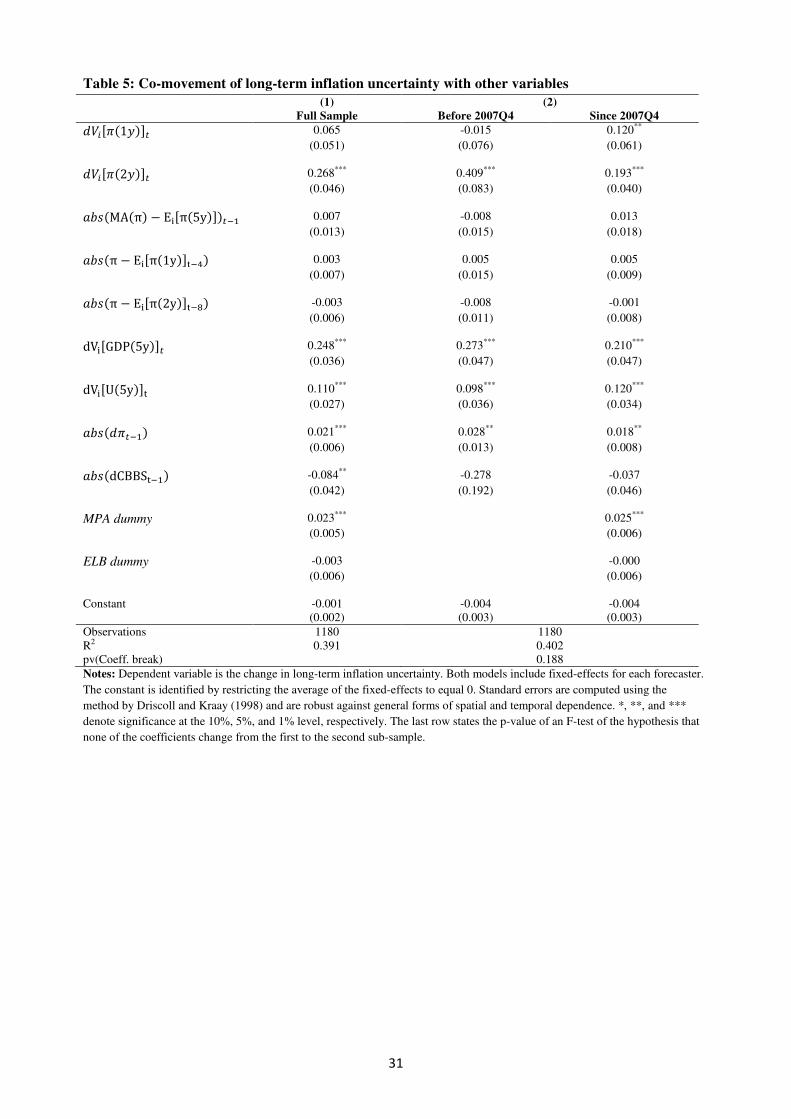
31
Table 5: Co-movement of long-term inflation uncertainty with other variables
(1) (2)
Full Sample Before 2007Q4 Since 2007Q4
<g�>�(1?)@� 0.065 -0.015 0.120**
(0.051) (0.076) (0.061)
<g�>�(2?)@� 0.268*** 0.409*** 0.193***
(0.046) (0.083) (0.040)
hi�(MA(π) − Ef>π(5y)@)�2� 0.007 -0.008 0.013
(0.013) (0.015) (0.018)
hi�(π − Ef>π(1y)@C2") 0.003 0.005 0.005
(0.007) (0.015) (0.009)
hi�(π − Ef>π(2y)@C2D) -0.003 -0.008 -0.001
(0.006) (0.011) (0.008)
dVf>GDP(5y)@� 0.248*** 0.273*** 0.210***
(0.036) (0.047) (0.047)
dVf>U(5y)@C 0.110*** 0.098*** 0.120***
(0.027) (0.036) (0.034)
hi�(<��2�) 0.021*** 0.028** 0.018**
(0.006) (0.013) (0.008)
hi�(dCBBSC2�) -0.084** -0.278 -0.037
(0.042) (0.192) (0.046)
MPA dummy 0.023*** 0.025***
(0.005) (0.006)
ELB dummy -0.003 -0.000
(0.006) (0.006)
Constant -0.001 -0.004 -0.004
(0.002) (0.003) (0.003)
Observations 1180 1180
R2 0.391 0.402
pv(Coeff. break) 0.188
Notes: Dependent variable is the change in long-term inflation uncertainty. Both models include fixed-effects for each forecaster.
The constant is identified by restricting the average of the fixed-effects to equal 0. Standard errors are computed using the
method by Driscoll and Kraay (1998) and are robust against general forms of spatial and temporal dependence. *, **, and ***
denote significance at the 10%, 5%, and 1% level, respectively. The last row states the p-value of an F-test of the hypothesis that
none of the coefficients change from the first to the second sub-sample.


