
0
Jobs and Income Growth of Top Earners and the Causes of Changing Income Inequality:
Evidence from U.S. Tax Return Data
Jon Bakija Bradley T. HeimWilliams College Office of Tax AnalysisWilliamstown, MA 01267 U.S. Department of [email protected] Washington, DC 20220 [email protected]
Preliminary Draft, March 17, 2009
Abstract: This paper presents summary statistics on the occupations of taxpayers in the top percentile of the national income distribution and fractiles thereof, as well as the patterns of real income growth between 1979 and 2005 for top earners in each occupation, based on information reported on U.S. individual income tax returns. The data demonstrate that executives, managers, supervisors, and financial professionals account for about 60 percent of the top 0.1 percent of income earners in recent years, and can account for 70 percent of the increase in the share of national income going to the top 0.1 percent of the income distribution between 1979 and 2005. During 1979‐2005 there was substantial heterogeneity in growth rates of income for top earners across occupations, and significant divergence in incomes within occupations among people in the top 1 percent. We consider the implications for various competing explanations for the substantial changes in income inequality that have occurred in the U.S. in recent times. We then use panel data on U.S. tax returns spanning the years 1987 through 2005, to estimate the elasticity of gross income with respect to net‐of‐tax share (that is, one minus the marginal tax rate). Information on occupation allows us to control for other influences on income in a flexible way using interactions among occupation, position in the income distribution, stock prices, housing prices, and the business cycle. We also allow for income shifting across years in response to anticipated tax changes, for the long‐run effect of a tax reform to differ from the short‐run effects, for heterogeneous mean‐reversion across incomes, and for heterogeneous elasticities across income classes. In a specification that does all this, we estimate a significant elasticity of 0.7 among taxpayers in the top 0.1 percent of the income distribution. Outside of the top 0.1 percent of the income distribution, we find no conclusive evidence of a positive elasticity of income with respect to net‐of‐tax shares. We find that the estimate for the top 0.1 percent is not robust to controlling for a spline in lagged income that is very flexible at the upper reaches of the income distribution, suggesting that the method used to allow for income dynamics is very important. Allowing for income shifting across years in response to anticipated tax changes has important consequences for the estimates. The views expressed are those of the authors and do not necessarily reflect those of the U.S. Department of the Treasury.

1
It is well known that the share of the nation’s income going to the top percentiles
of the income distribution in the United States has increased dramatically over the past
three decades. Data from individual income tax returns tabulated by Piketty and Saez
(2003, updated 2008) and shown in Figure 1 demonstrates that the percentage of all pre‐
tax income (excluding capital gains) in the United States that was received by the top 0.1
percent of income earners rose strikingly from 2.2 percent to 8.0 percent between 1981
and 2006. But until now, there has been little hard data available to the public on what
these people typically do for a living, which is an economically important question.
Kaplan and Rauh (2009) estimate what share of tax returns at the top of the income
distribution can be accounted for through publicly‐available information on top
executives of publicly‐traded firms, financial professionals, law partners, and
professional athletes and celebrities. Despite making various extrapolations beyond
what is directly available in publicly‐available data sources, for the year 2004 they are
only able to identify the occupations of 17.4 percent of the top 0.1 percent of income
earners. As Kaplan and Rauh, among others (e.g., Gordon and Dew‐Becker, 2008) have
emphasized, the questions of what proportion of people in the top income percentiles
are in different occupations, and how these proportions have been changing over time,
have important implications for evaluating competing explanations for the rapid rise in
incomes at the top. Yet until now we have had very incomplete information on these
questions. One contribution of our paper is to present summary statistics tabulated
from cross‐sectional individual income tax return data at the U.S. Treasury Department
on what share of top income earners work in each type of occupation, the shares of top
incomes that are accounted for by the various occupations, mean incomes of top earners
in each occupation, and how all of these have changed over selected years between 1979
and 2005. Through this method we are able to account for the occupations of almost all
top earners – for example, for over 99 percent of primary taxpayers in the top 0.1 percent
of the income distribution in 2004.
The second contribution of our paper is to use panel data on U.S. federal income
tax returns spanning the years 1987 through 2005, which includes information on the

2
occupation and industry of each taxpayer, to try to distinguish empirically the causal
impact of marginal income tax rates, which affect the incentive to earn income, from
other possible explanations for the rise in top incomes. We estimate the elasticity of
gross income with respect to net‐of‐tax share (that is, one minus the marginal tax rate).
Information on occupation allows us to control for other influences on income in a
flexible way using interactions among occupation, position in the income distribution,
stock prices, housing prices, and the business cycle. We also allow for income shifting
across years in response to anticipated tax changes, for the long‐run effect of a tax
reform to differ from the short‐run effects, and for heterogeneous elasticities across
income classes.
Our panel data analysis contributes to the now voluminous literature on the
“taxable income elasticity,” recently and comprehensively reviewed by Saez, Slemrod,
and Giertz (2009). Early and influential papers by Feldstein (1995, 1999) argued that the
responsiveness of taxable income to changes in marginal tax rates provides information
on nearly all of the margins along which individual taxpayers may adjust their behavior
to avoid taxes – not only changes in hours worked, but also changes in work effort per
hour, form of compensation, choice of tax‐deductible consumption versus non‐
deductible consumption, risk taking and entrepreneurship, and so forth. Feldstein went
on to argue that under certain assumptions, the elasticity of taxable income with respect
to the net‐of‐tax‐share can be a sufficient statistic to calculate the deadweight loss caused
by income tax.1 It turns out that seemingly small differences in this elasticity have
dramatically different implications for the amount of deadweight loss caused by
taxation. Giertz (2009) performs simulations using published tax return data, and his
analysis suggests that given the current structure of taxation in the U.S., if the taxable
income elasticity is 0.2, the marginal deadweight loss per additional dollar of revenue
raised in the top tax bracket is $0.31 and the peak of the Laffer Curve occurs at a tax rate
of 78 percent. If the elasticity is 0.8, the deadweight loss caused by raising one additional 1 See, however, Chetty (2008) and Saez, Slemrod, and Giertz (2009) for discussion of why these assumptions may not hold.

3
dollar of revenue from a top‐bracket taxpayer is $6.57, and the peak of the Laffer curve
occurs at a tax rate of 41 percent, which is only slightly above the top marginal income
tax rate that is scheduled to apply when the federal tax cut enacted in 2001 (EGTRRA)
expires.
The behavior and incomes of very‐high income people are of extreme
quantitative importance for government revenue and for the economy, which is one
motivation for our focus on their incomes in this paper. Mudry and Bryan (2009) report
that the top one percent of taxpayers ranked by income paid 40 percent of federal
personal income taxes in 2006, and the top 5 percent of taxpayers paid 60 percent of
federal personal income taxes. This is explained by a combination of the effective
progressivity of the personal income tax, and the large share of national income earned
by people at the top of the distribution.2
In our cross‐sectional analysis, we find that executives, managers, supervisors,
and financial professionals account for about 60 percent of the top 0.1 percent of income
earners in recent years, and can account for 70 percent of the increase in the share of
national income going to the top 0.1 percent of the income distribution between 1979
and 2005. During 1979‐2005 there was substantial heterogeneity in growth rates of
income for top earners across occupations, and significant divergence in incomes within
occupations among people in the top 1 percent. Using panel data, we estimate a
significant elasticity of 0.7 among taxpayers in the top 0.1 percent of the income
distribution. Outside of the top 0.1 percent of the income distribution, we find no
conclusive evidence of a positive elasticity of income with respect to net‐of‐tax shares.
However, we find that the estimate for the top 0.1 percent is not robust to controlling for
a spline in lagged income that is very flexible at the upper reaches of the income
distribution, suggesting that the method used to allow for income dynamics is very
important. In addition, allowing for income shifting across years in response to
anticipated tax changes has important consequences for the estimates.
2 In fiscal year 2007 federal personal income tax revenues were $1.16 trillion, or 45 percent of federal revenues. Source: Economic Report of the President (2009).

4
The paper proceeds as follows. In the following section, we review the literature
on the causes of changing income inequality and its implications for estimating taxable
income elasticities. We then describe the two sources of tax data that we use in the
empirical work. The following section outlines results tabulating occupations and
incomes of high income taxpayers, and the section after that presents some resuts from
preliminary estimates of the elasticity of taxable income accounting for the occupations
of high income earners. The last section concludes.
Literature Review
The literature on the causes of rising income inequality over the past few decades
has identified many factors that may contribute to rising top income shares. First, it is
important to note that Piketty and Saez (2003, updated 2008), among others, have shown
that wage and salary income, as well as self‐employment income and closely‐held
business income that largely reflect labor compensation, now account for the vast
majority of the incomes of top income earners, and have also been growing substantially
as a share of that income in recent decades.3 So theories to explain the rising top income
shares shown in Figure 1 must largely be about compensation for labor.
One explanation for rising income inequality emphasizes that it coincided with
advancing globalization, as indicated for example by increasing shares of imports and
exports in GDP. This may increase the demand for the labor of high‐skill workers in the
U.S., because they can now sell their skills to a wider market, and highly‐skilled workers
are scarcer in the rest of the world than in the U.S. Globalization may similarly depress
wages for lower‐skilled workers, because they now have to compete with abundant low‐
skill workers from the rest of the world (Stolper and Samuelson, 1941; Krugman 2008).
3 For example, even among the top 0.01 percent of income recipients in 2005, salary income and business income (that is, self‐employment income, partnership income, and S‐corporation income) accounted for 80 percent of income excluding capital gains, and 64 percent of income including capital gains. Those figures were 61 percent and 46 percent, respectively, in 1979. (Source: authors’ calculations based on data posted by Emanuel Saez at <http://elsa.berkeley.edu/~saez/TabFig2006.xls>).

5
A second hypothesis is skill‐biased technical change (Katz and Murphy, 1992; Bound
and Johnson, 2002; Card and DiNardo, 2002; Garicano and Rossi‐Hansberg 2006;
Garicano and Hubbard 2007). Technology has arguably changed over time in ways that
complement the skills of highly‐skilled workers, and substitute for the skills of low‐
skilled workers. A third hypothesis, closely related to the previous two, is the
“superstar” theory suggested by Sherwin Rosen (1981). In this theory, compensation for
the very best performers in each field rises over time relative to compensation for others,
because both globalization and technology are enabling the best to sell their skills to a
wider and wider market over time, which displaces demand for those who are less‐than‐
the best. This is easiest to see for entertainers, but could easily apply to other
professions as well.
A fourth hypothesis is that the increasing inequality may be explained to some
extent by executive compensation practices (Bebchuk and Walker, 2002; Bebchuk and
Grinstein, 2005; Eissa and Giertz, 2009; Friedman and Saks, 2008; Gabaix and Landier,
2008; Gordon and Dew‐Becker, 2008; Kaplan and Rauh 2009; Murphy 2002; Piketty and
Saez 2006). A large share of executive pay comes in the form of stock options, and
almost all stock options are treated as wage and salary compensation on tax returns
when they are exercised (Goolsbee 2000).4 Because of this, the values of stock options
exercised by employees are generally counted in the measures of income used in the
income inequality literature. 5 It is clear that executive compensation has increased
greatly over time, but there is a raging debate over why this has happened, and whether
there are enough executives for this to explain much of the rise in top income shares.
4 Federal income tax law classifies compensation in the form of stock options into two categories. “Non-qualified” stock options are treated as wage and salary income when exercised. “Incentive” stock options are taxed as capital gains a the personal level when exercised, but are denied a deduction for labor compensation from the corporate income tax. Under current law, the non-qualified options are generally much preferable from a tax standpoint compared to incentive stock options and Goolsbee (2000) indicates that almost all stock options used in executive compensation are of the non-qualified type. However, before 1986 incentive stock options were less tax disadvantaged. 5 The taxable income elasticity and inequality literatures usually focus on income excluding capital gains, because we usually only have data on gains realizations (rather than accruals) reported on tax returns, because capital gains realizations fluctuate wildly over time, because capital gains receive different tax treatment than other income, and because capital gains have obvious alternative explanations (e.g., stock market booms and busts).

6
Bebchuk and Walker (2002) and Bebchuk and Grinstein (2005), among others, have
argued that high and rising executive pay reflect the fact that the pay of executives is set
by their peers on the board of directors, that free rider problems prevent shareholders
from doing sufficient monitoring of executive compensation practices, and that the
problems have been getting worse over time. Many others (for example, Murphy 2002)
argue that executive pay reflects economically efficient compensation necessary to align
executive incentives with those of shareholders. Gabaix and Landier (2008) argue that
the increasing scale of firms has been critical to explaining rising executive pay;
however, Friedman and Saks (2008) show that real executive pay grew very little
between World War II and the mid‐1970s despite large increases in firm size during that
period, casting doubt on the Gabaix and Landier hypothesis.
A fifth hypothesis is that technological change and compensation practices in
financial professions play a critical role. Philippon and Reshef (2009) show that the skill‐
intensity of financial sector jobs has grown dramatically since the early 1980s.
Moreover, they estimate that since the mid‐1990s, financial sector workers have been
capturing rents that account for between 30 and 50 percent of the difference between
financial sector wages and wages in other jobs. Of course, compensation of executives,
financial professionals, and perhaps top earners in other fields (such as high technology)
can be expected to be heavily influenced by financial market asset prices, particularly
stock prices, which went up dramatically at the same time as the increase in inequality.
So part of the rising inequality may simply reflect that people in these professions have
compensation that is strongly tied to the stock market, and got lucky when the stock
market went way up. This might be counted as a separate hypothesis or a subset of the
previous two.
Another hypothesis related to the past few is that social norms and institutions in
the United States may be changing over time in a way that reduces opposition to high
pay (see, e.g., Piketty and Saez 2006). For example, perhaps the “outrage constraint”
once played and important role in preventing executives and their peers on the board
from colluding to grant excessively high pay, but social norms against high pay have

7
weakened over time so this constraint no longer binds. Alternatively, perhaps the social
norms of old were harming efficiency by preventing corporate boards from granting
stock options that were sufficiently large to align the incentives of the executive with
those of the shareholders.
Yet another hypothesis brings us back to taxes. Prior to TRA86, top personal
income tax rates exceeded the top corporate income rate by a wide margin, so there was
a strong incentive to organize one’s business as a C‐corporation, because it enabled one
to defer paying high personal tax rates on one’s income as long as it was retained within
the corporation, at the cost of paying the lower corporate rate right away. After TRA86,
the top personal rate was reduced below the top corporate rate, which created an
incentive to change one’s business to a pass‐through‐entity such as an S‐corporation, the
income of which is taxed only once at the personal level. This has important
implications for the income inequality and taxable income elasticity literatures, because
it suggests that part of the difference in top incomes before and after 1986 does not
reflect the creation of new income, but rather income that was previously not reported in
the data (which is derived from personal income tax returns) and now is. Slemrod
(1996) and Gordon and Slemrod (2000) demonstrate that this factor must explain a
substantial portion of the increase in top incomes around 1986. Yet, looking back at
Figure 1, even if one restricts attention to the period from 1988 forward, the income
share of the top 0.1% still increased from 5 percent of national income to 8 percent.
Taxable income elasticity researchers studying periods spanning 1986 try imperfect
methods for dealing with this such as omitting returns with any S‐corporation income.
One advantage of focusing our gross income elasticity analysis on panel data starting in
1987 is that it will be less subject to this problem.
One particularly promising development for the prospects of distinguishing
which explanations for increasing income inequality are correct has been the collection
of long historical time‐series on top income shares in a variety of nations. Figure 1
shows the share of income going to the top 0.1 percent of the income distribution in the
U.S., France, and Japan, based on data from Piketty and Saez (2006, updated in 2008),

8
Moriguchi and Saez (2008), Piketty (2003), and Landais (2008). It shows that while the
share going to top earners increased dramatically between 1981 and 2006 in the U.S., it
was basically flat in these other countries until very recently. There is evidence of some
increase in top income shares in Japan and France since the late 1990s, but the changes
are far less pronounced than what has occurred in the U.S. Various authors (Atkinson,
2007; Atkinson and Salverda, 2005; Saez and Veall, 2005; and many other studies cited in
Atkinson and Piketty, 2007, Saez 2006 and Roine, Vlachos, and Waldenstrom 2008) have
constructed top income shares for other countries as well, and have shown that top
income shares have grown sharply only in English speaking countries. Like France,
other continental European countries have had flat top income shares in recent decades,
with moderate upward trends beginning to emerge only after the late 1990s in countries
such as France and Spain where very recent data is available.
The international data on top income shares seems inconsistent with some of the
theories for rising income inequality cited above, and only partly consistent with others
(Piketty and Saez 2006). For example, it is hard to see why globalization and skill‐biased
technological change would raise top income shares sharply in English speaking
countries but not in Continental Europe or Japan where the degree of globalization and
technological advancement is presumably similar. Regarding the tax hypotheses, Figure
2 shows that there were much larger and earlier cuts in top marginal income tax rates in
the U.S. than in France, and in general English speaking countries had much larger
reductions in top marginal income tax rates than did Continental European countries.
So the fact that top income shares went way up in the English speaking countries but not
in Continental Europe seems to support the theory that marginal income tax rates are an
important part of the explanation for surging top income shares in English speaking
countries. However, Figure 2 also shows that Japan had similarly large reductions in
top marginal income tax rates to the U.S. since 1981, yet no increase in top income shares
happened there, which is highly inconsistent with the tax‐based theories.
Theories about executive compensation, financial market asset prices, social
norms, and institutions seem to fit the data better, but have been hard to prove. While

9
Japan and the U.S. had similar changes in tax rates, an important difference between
them is that it was illegal to compensate executives with stock options in Japan until
1997 (Bremner 1999). Executive stock options are legal in France, and stock prices went
up in France too; but average executive compensation in France is less than half of what
it is in the U.S., which might be explained by social norms (The Economist, 2008, and
Alcouffe and Alcouffe 2000). This could explain why top income shares seem largely
unaffected by stock prices in France. Kaplan and Rauh (2009), on the other hand, have
argued that executives of publicly‐traded firms represent too small of a share of top
income earners in the U.S. to be able to explain much of the rise in top income shares.
Part of the motivation of our present study, therefore, is to see whether more complete
information on the occupations of high earners might corroborate what seems to be
happening in the international data. The role of financial market asset prices in
influencing top income shares is corroborated by Roine, Vlachos, and Waldenstrom
(2008), who estimate regressions on cross‐country data from a large number of years and
find that top income shares are strongly positively correlated with stock market
capitalization; they also find that higher marginal income tax rates are associated with
smaller top income shares, although their tax measures are rough.
Clearly, a researcher wishing to distinguish the causal impact of marginal tax
rates on income from all the other possible explanations listed above faces a difficult
task. Contributors to the taxable income elasticity literature have tried various clever
but imperfect methods to try to control for the kinds of factors discussed above.
First is the use of the standard difference‐in‐differences identification strategy (or
more generally the use of fixed effects or differencing together with year dummies). But
for reasons detailed above, this is almost certainly insufficient to address the kinds of
omitted variable bias stories we have been talking about.
Feldstein analyzed the effect of the Tax Reform Act of 1986 (TRA86) on taxable
income and gross pre‐tax income. Feldstein applies a difference‐in‐differences
approach, where people with high tax rates before the reform were the “treatment
group” because they experienced a large cut in marginal tax rates (up to 50 percent

10
before the reform and a maximum of 28 percent afterwards) and those with lower tax
rates before the reform, who experienced only small marginal tax rate cuts, were the
“control group.” As is apparent from Figure 1, in the years around TRA86, pre‐tax
incomes of high‐income people grew much faster than those of other people. As a result,
Feldstein estimated a very large elasticity of income with respect to the net‐of‐tax share,
in some cases in excess of one.
Feldstein’s study also illustrates some of the challenges involved in
distinguishing the causal effect of taxes from the effects of other factors that also
influence income. In Feldstein’s simple diff‐in‐diffs analysis, which did not control for
other factors, the key identifying assumption was that there were no other factors
besides taxes that influence income that were changing in different ways over time for
people at different income levels, because whether someone experienced a change in tax
rates was determined largely by the starting level of income before the reform.
Therefore, the taxable income elasticity literature in public economics is inextricably
intertwined with the literature on the causes of changing income inequality. As Figures
1 and 2 show, between 1981 and 2006 incomes of very high‐income people rose sharply
relative to the incomes of the rest of the population, while at the same time top marginal
income tax rates were cut sharply, from 70 percent in 1980 to 35 percent as of 2006.
Looked at over the period as a whole, the data appears consistent with the theory that
high‐income people respond to the improved incentives to earn income created by tax
cuts, although there are some features of the data, such as the fact that the incomes at the
top of the distribution continued to rise sharply after an increase in the to marginal tax
rate from 31 percent to 39.6 percent starting in 1993, which do not seem particularly
consistent with the theory. But of course, many other factors that might influence top
incomes and income inequality were also changing over time.
Gruber and Saez (2002) supplemented the difference‐in‐differences approach by
controlling for a ten‐piece spline in log income from the first year of a three year
difference. This effectively controls for unobservable influences on income that follow a

11
different linear time trend at each point in the income distribution, allowing for the rate
of change in the effect with respect to income to differ for each decile of the distribution.
The use of the spline in income was also motivated by the apparently large degree of
mean‐reversion in income, which makes it difficult to distinguish the effect of a change
in taxes from the effects of transitory fluctuations in income over time, together with the
observation that the degree of mean‐reversion appears to be heterogeneous across the
income spectrum. Much of the subsequent literature has followed suit. However, we
demonstrate below that whatever unmeasured factors are driving the rise in top income
shares, they cannot possibly be well‐described by a linear time trend.
Another approach, used for example in Auten and Carroll (1999) and Auten,
Carroll, and Gee (2008), has been to make use of internal government panel data on tax
returns that includes information on occupation in selected years. These authors
controlled for occupation dummies in specifications that differenced the data over time,
which effectively controls for a different linear time trend in unmeasured influences
affecting income for each occupation, but did not control for a spline in lagged income.
There is abundant evidence from the labor economics literature that increases in
earnings inequality have been “fractal” in nature – almost regardless of how you define
a group, including by occupation, earnings inequality has been increasing within that
group (see, for example, the survey by Levy and Murnane, 1992). We demonstrate
below that there has been substantial divergence in incomes within the same occupation
even among people who are in the top one percent of the income distribution (which to
our knowledge has not previously been demonstrated in the labor literature, due to top
coding of publicly available earnings data). For these reasons, the approach used in
prior taxable income elasticity papers that had information on occupation may have
been insufficient to effectively control for unmeasured time‐varying influences on
income. Those papers also used short panels that each spanned only a single federal tax
reform that moved tax rates in one direction (1985 and 1999 in Auten and Carroll, 1999
through 2005 in Auten, Carroll, and Gee), which makes it difficult to distinguish the
effects of tax changes from mean reversion in income and from unmeasured time‐

12
varying influences. In our econometric analysis we use panel data spanning the years
1987 through 2005, which includes both major tax increases and tax cuts, and we will try
various methods of controlling for time‐varying non‐tax influences on income, including
ones that are considerably more flexible than those used in the previous literature, and
we show that this has important impacts on the estimates. Moreover, prior papers using
tax data matched with occupational information did not share much information about
those occupations aside from sample means and regression coefficients. We show that
there is much more that can be learned from a detailed analysis of that data.
As noted above, the elasticity of taxable income to the net‐of‐tax share can be
used to estimate revenue impacts of tax changes and to calculate the deadweight loss of
the income tax. Another elasticity of interest is the elasticity of gross income with
respect to the net‐of‐tax share (also called the “gross income elasticity”); this is useful for
calculating the deadweight loss of taxation in the same way as the taxable income
elasticity is, except that it leaves out the behavioral margin of switching between non‐
deductible to deductible consumption. In this paper we focus on the gross income
elasticity because that is most relevant to the question of whether the increases in gross
income inequality shown in Figure 1 can be explained by behavioral responses to
marginal tax rates; the debate over the causes of rising income inequality debate has
mainly been about gross income, not taxable income. Moreover, calculations of
deadweight loss based on the taxable income elasticity will tend to overstate deadweight
loss when some items of deductible consumption (for example, charitable contributions)
involve positive externalities (Saez, Slemrod, and Giertz 2009).6
6 The taxable income elasticity literature often finds that the taxable income is more elastic than gross income with respect to the net‐of‐tax share (see, e.g., Gruber and Saez 2002). In Bakija and Heim (2008) we estimate that charitable contributions among high‐income people are highly elastic with respect to marginal tax rates. This suggests that charitable contributions might be an important part of the explanation for why taxable income elasticities tend to be larger than gross income elasticities.
13
Data
For this paper, we utilize both repeated cross‐sections of tax returns and a panel
of tax returns.
The repeated cross‐section dataset was created by merging files produced by the
Statistics of Income (SOI) division of the Internal Revenue Service. Each year, a
stratified random sample of tax returns is drawn, where the probability of being selected
increases with income, and the highest income returns are selected with certainty.7 As a
result, these cross‐sections contain complete tax return information from the highest
income taxpayers in each year. Variables are collected from Form 1040 and many of the
supporting schedules, and include wages and salaries, dividends and interest, capital
gains, and income from closely held businesses.
Occupation and industry data were then merged together with these datasets.8
Each year since 1916, taxpayers have been asked to identify their occupation on their
federal tax form, with the current single line entry format beginning in 1933.9 In 1979,
SOI began a pilot project to convert the text entries from the tax forms to standard
occupation codes (SOC’s). Following the pilot project, they attempted to code
occupations for the entire 1979 cross‐sectional file (both primary and secondary filers, if
applicable) according to the 1972 SOC classification system. To aid in this, information
on the industry of the taxpayer’s employer was merged into the dataset by matching the
employer identification number (EIN) from the taxpayer’s W‐2 form to industry codes
7 In 2004, for example, 100 percent of returns with incomes above $5 million are included in our cross‐sectional sample. In order to avoid disclosure, the publicly‐available versions of the cross‐sectional tax return data sample even the highest income returns, and some variables from these returns are withheld or blurred. For example, in the 2004 public‐use data, 33 percent of returns with incomes above $5 million are included (Weber 2007). 8 The creation of the occupation datasets is described in Crabbe, Sailer, and Kilss; Sailer, Orcutt, and Clark; Clark, Riler, and Sailer; and Sailer and Nuriddin. 9 This history is described in Sailer, Orcutt, and Clark. As noted by Sailer and Nuriddin, essentially no guidance is given to taxpayers on how to describe their occupation, and no categories are given from which taxpayers can choose.

14
from the Social Security Administration’s Employer Information File, allowing
identification of the taxpayer’s industry of employment as well.
Occupations and industries were coded intermittently in the subsequent years,
with an occupation file created for the 1993, 1997, and 1999 tax years, where the samples
in 1993 and 1999 contained taxpayers in both the cross‐section and panel datasets from
those years. Starting in 2001, occupations and industries have been coded every year,
with the most recent data coming from 2005. Across all years, occupations were coded
for 90 percent of working primary filers and 84 percent of working secondary filers, and
industries were coded for 87 percent of working primary filers and 77 percent of
working secondary filers.
Because the occupation and industry classification systems changed a number of
times,10 to make the codes comparable across time we converted occupation codes in
each year to the equivalent 2000 SOC code, and industry codes to the equivalent 1997
NAICS code. To make the occupation and industry data more amenable to studying
occupations and industries that have been the focus of previous studies, we then
aggregated these occupation codes into 22 occupation groups and industry codes into 11
industry groups. The occupation groupings are detailed in Appendix Table A.1.
Aggregating the data in this manner also helps reduce noise that might come from
taxpayers changing the description of their occupation from year to year. When looking
at the very highest income groups we further aggregate occupations to prevent any cell
from becoming too small.
We use different measures of income in the analysis. For our measure of gross
income, we use reported adjusted gross income (AGI) less social security income,
unemployment income, and state tax refunds, and add back total adjustments less half
of self‐employment taxes. To keep this measure consistent across years, in 1979 we add
60 percent of long‐term capital gains and excluded dividends and interest. We also
10 The 1980 SOC codes were used for the 1979 through 1997 files, and 2000 SOC codes were used for the 1999 through 2005 files. The 1972 SIC codes were used for the 1979 file, 1980 SIC codes were used for the 1993 and 1997 files, 1997 NAICS codes were used for the 1999 and 2001 files, and 2002 NAICS codes were used for the 2002 through 2005 files.
15
create a measure of gross income excluding capital gains, and following the previous
literature focus mainly on that. Our measure of “labor and business income” adds
together wages and salaries, income from sole proprietorships, and income from
partnerships and S‐corporations. Finally, wage and salary income comes from the
relevant line from Form 1040.
Sample statistics from the merged cross‐section file are presented in Appendix
Table A.2. The mean income in the cross‐section file is in excess of $1.5 million, though
when capital gains are excluded, this figure drops to $834,490. About 25 percent of the
sample derived a majority of their combined salary and business income from a closely
held business, and 66 percent of the taxpayers in the sample were married.
Appendix Table A.3 presents the distribution of occupations among all primary
and secondary filers in the pooled cross‐section sample. For primary filers, the largest
occupations are blue collar and miscellaneous (largely low‐skill) service occupations
(17.4 percent), executives (9.0 percent), and financial professions (6.6 percent).
Taxpayers were either not working or deceased for 10.8 percent of the pooled cross‐
section sample, and occupations could not be identified for 8.6 percent of returns.
In both the cross‐sectional and panel analyses, we need to assign tax returns to
percentiles of the national income distribution (including non‐taxpayers). For each year
we sort returns in the internal Treasury cross‐sectional data set in descending order by
income and count down to compute the number of returns that represent a particular
percentage of the total number of tax units in the United States for that year. We then
determine the minimum income for that group and use it to assign people to
percentiles.11 The minimum income levels to qualify for the top quantiles of the
distribution of income (excluding capital gains) in 2005 (measured in constant year 2007 11 A “tax unit” is defined as a married couple or a single adult aged 20 or over, whether or not they file an income tax return. Data on total number of tax units is taken from Piketty and Saez (2003, updated 2008). Our thresholds for percentiles of the income distribution match up fairly closely to those reported in Piketty and Saez. Their estimates are based on public‐use micro datasets of tax returns up through 2001 and interpolations from published tables thereafter. In this preliminary version of our paper we use the thresholds reported in Piketty and Saez to assign returns in the panel to percentiles, because we have not yet computed thresholds from cross‐sectional data for all years included in the panel.

16
dollars and rounded to the nearest thousand) were: $94,000 for the top 10 percent;
$129,000 for the top 5 percent, $295,000 for the top 1 percent, $450,000 for the top 0.5
percent, and $1,246,000 for the top 0.1 percent.
The panel of tax returns was created by merging three separate panels. 12 The
first panel was collected from 1987 through 1996, and is known as the Family Panel.13
This panel consists of two segments. The first is a cohort segment that was created by
drawing a stratified random sample of taxpayers (including spouses and dependents)
who filed in tax year 1987 and following them over the next nine years. This segment
includes a random sample of taxpayers chosen because the primary taxpayer’s SSN
ended in one of two 4‐digit combinations (known as the Continuous Work History
Subsample), and a sample of taxpayers for whom sampling probabilities increased with
income. The second segment is a refreshment segment consisting of taxpayers with one
of the two CWHS SSN endings, who filed in at least one tax year between 1988 and 1996
but who were not filers in 1987. Overall, the Family Panel consists of 1.26 million
returns, and spans the Ominibus Budget Reconciliation Acts of 1990 and 1993 (OBRA90
and OBRA93) as well as covering the end of the phase‐in of TRA86.
The second panel was collected from 1999 through 2005, and is known as the
Edited Panel.14 This panel consists of a stratified random sample of tax returns drawn in
1999 (including a CWHS subsample comprised of taxpayers who had one of five 4‐digit
SSN endings, and a high income subsample), for which the primary and secondary filers
were followed over the subsequent six years. This panel consists of more than 550,000
tax returns, and spans the two most recent major tax changes, the Economic Growth and
Tax Relief Reconciliation Act (EGTRRA2001) and the Jobs and Growth Tax Relief
Reconciliation Act of 2003 (JGTRRA2003).
To bridge the years between these two panels, a third panel was created by
drawing from the 1997 and 1998 SOI cross‐sectional files those taxpayers who had
12 Some of the following discussion of the panel data draws from our discussion of similar data in Bakija and Heim (2008). 13 For more information on the Family Panel, see Cilke et al. (1999, 2000). 14 For more information on the 1999‐2005 Edited Panel, see Weber and Bryant (2005).

17
primary filers with one of the two CWHS endings in 1997 (or one of the five CWHS
endings in 1998). This panel comprises over 67,000 tax returns.
Since occupation information was not coded for all years of the panel, we impute
occupations to observations from these years using information from other years. To do
this, we assign to each observation the occupation from the closest year in which an
occupation is observed. If there is a tie, we take the occupation from the earlier year.
Marginal tax rates and tax liabilities in this study were calculated using the
comprehensive income tax calculator program described in Bakija (2008), and include
both state and federal income taxes and Social Security and Medicare payroll taxes. The
calculator incorporates such details as the minimum and alternative minimum taxes,
maximum tax on personal service income, and income averaging in the years when
these were applicable.15 Marginal tax rates were calculated by incrementing wages and
salaries by ten cents, calculating the marginal increase in taxes owed, and dividing that
by the ten cents.16
For the estimation using the panel file, several cuts were made. All dependent
filers and all taxpayers under the age of 25 were dropped from the panel sample, as
were married taxpayers who filed separately and taxpayers with missing data on state
of residence. To remove returns with internally inconsistent data, we dropped from the
panel any returns where the federal income tax liability reported on the return was not
sufficiently close to federal income tax liability figured by the tax calculator.17 Since we
15 For some returns in 1979‐95 panel, we used an iterative process to back out certain items needed for income averaging and AMT computations from the reported liabilities for those taxes. 16 Taxes incorporated into our marginal tax rate variable include both federal and state personal income taxes as well as federal Social Security and Medicare payroll taxes. Let mtr be the marginal personal income tax rate computed as described above, and ssmtr be the combined employer and employee payroll tax computed as described above. Our marginal tax rate variable is (mtr + ssmtr)/[1 + (ssmtr/2)]. This represents the marginal increase in tax liability caused by earning another dollar of wage and salary income including the employer payroll tax contribution. For consistency, we add employer social security contributions to our income variable when we use it in the econometric analysis, but not in the descriptive statistics. 17 Specifically, we cut observations if the federal tax liability before credits and minimum taxes computed by the tax calculator differs from the amount reported in the dataset by more than $10,000. Also note that before doing this, we made extensive efforts to resolve internal

18
use information from two year lags and one year lead, we exclude any observations for
which any of these leads or lags are missing.
We sometimes need to impute occupations across years for an individual, and
we wish to avoid incorrectly imputing an occupation to someone who is no longer
working. So we drop returns where the primary taxpayer (who is male 90 percent of the
time in our panel sample) is likely to be out of the labor force. In addition to dropping
people whose occupation codes indicate they are not working in the years we have
occupation codes, we also drop from the panel sample returns where the primary
taxpayer is aged 65 or above. Returns with income excluding capital gains, or sum of
salary income and business income, less than $10,000 are also dropped. Retirement and
labor force participation are one margin along which behavior may respond to taxes, so
our estimates will not reflect that particular kind of behavioral response.
We then drop anyone with an occupation that either tends not to earn a high
income or which represents a very small share of top income earners (including farmers
and ranchers, pilots, government workers, teachers, social workers, blue collar workers,
and miscellaneous service professions). This is done because we are trying to explain
why top income shares are rising, and because we want the people in our sample who
experienced little or no change in tax rates to be a good control group (in the sense of
providing an accurate counterfactual) for the high‐income people who experienced large
changes in tax rates. We choose to drop people from the sample based on occupation
rather than income (except for the very low $10,000 threshold) because selecting the
sample on income can be a source of bias when there is mean‐reversion. Under a
selection rule based on income, people with positive transitory shocks to income will be
more likely to be selected and will subsequently experience income declines, while
people with negative transitory shocks to income (who therefore subsequently
experience increases in income) are less likely to be selected. Our data confirm that
inconsistencies in the data by inferring values of problematic variables from information available elsewhere on the return.

19
occupation (as we have defined it) tends to be far more stable over time than income, so
using occupation for selection is far less likely to produce this problem.
The final panel estimation sample comprises 244,909 observations. Sample
statistics are presented in Appendix Table A.4. As evidence of the large number of high
income taxpayers represented in this sample the mean amount of income (excluding
capital gains) is $1.1 million. Over 80 percent of the sample is married, with the mean
age of the primary filer being 46. Executives make up 15.0 percent of the sample, with
managers comprising 13.1 percent and those working in finance comprising 10.6
percent. Numbers and shares of observations in the panel sample used for estimation
that fall into each quantile are shown in appendix table A.5. Twenty percent of the panel
estimation sample, or 50,127 tax returns, are in the top 0.1 percent of the income
distribution.
Occupations and Incomes of High Income Taxpayers
Table 1 reports the percentages of primary taxpayers that are in each occupation
among the top 0.1 percent of income earners, from the 2004 cross‐sectional tax data, and
compares it to estimates of the same thing by Kaplan and Rauh (2009) that were based
on extrapolations from publicly‐available data. For comparability with Kaplan and
Rauh, in this table we rank taxpayers by income including capital gains. In the tax data,
occupation is known for all but 0.7 percent of these taxpayers. In comparison, Kaplan
and Rauh, using data from a variety of different sources, are able to identify occupations
for about 17.4 percent of this income group. It also appears that the shares of
occupations that Kaplan and Rauh study comprise a greater share in the tax data than
was found in their paper. In the tax data, 18.4 percent of the top 0.1 percent of the
income distribution had financial professions (including financial executives, managers,
and supervisors), 6.2 percent were lawyers, and 3.1 percent were in the arts, media or
sports, while in their data sources, Kaplan and Rauh were able to identify 10.3 percent of
the top 0.1 percent of the income distribution coming from financial professions, 2.4

20
percent employed in law firms, and 0.9 percent having an occupation in arts, media or
sports.
Kaplan and Rauh were able to identify 3.8 percent of the top 0.1 percent of
income as top non‐financial executives in publicly traded firms. Based on this, they
argued that executives represent too small of a share of top income earners for corporate
governance issues and stock options to be a good explanation for rising top income
shares. Our tax data does not contain information about the ownership structure of the
firm for which the taxpayer works, but over 40.8 percent of the top 0.1 percent report
their occupation as being an executive, manager, or supervisor of a firm in a non‐
financial industry, and 28.6 percent report being an executive. Undoubtedly, many of
these executives work for closely‐held businesses rather than large publicly traded
firms. To investigate this issue, we attempt an approximate division of executives,
managers, and supervisors into “salaried” versus “closely held business” categories. An
executive, manager or supervisor is assigned to the “closley held business” category if
the sum of primary earner self‐employment income, and partnership and S‐corporation
income for the return as a whole, exceeds wage and salary income on the return.
Otherwise, the executive is assigned to the “salaried” category. Among managers and
supervisors in the “salaried” category, wages and salaries represent 94 percent of
combined labor and business income reported on the tax return; the corresponding
figure for those in the “closely held business” category is only 12 percent, so this method
of division appears to work well. We would expect that those in the “salaried” category
are likely to be working for publicly‐traded corporations, or at least large closely‐held
corporations. Salaried non‐financial executives account for 15 percent of the top 0.1
percent, and salaried managers represent another 4.7 percent, for a total of about 20
percent. The vast difference between this and Kaplan and Rauh’s 3.8 percent figure
might be explained partly by non‐publicly‐traded firms, to the extent that executives
and managers of these firms receive most of their income from wages and salaries.
Some of the difference must also be due to the fact that Kaplan and Rauh only look at
the top 5 executives at each firm, and some may be due to other income of executives

21
and managers that is not disclosed in public documents but which is included on their
tax returns. This suggests that corporate governance issues and stock options may be
more important for explaining top income shares than Kaplan and Rauh suggested.
Moreover, while principal‐agent problems may be smaller in closely‐held firms, they are
not always absent, and executives and managers of closely held firms are sometimes
compensated with stock options, so that financial market asset prices may be important
for explaining their pay. Later in the paper, we demonstrate that the incomes of
executives, managers, and supervisors in the top 0.1 percent of the income distribution
are highly sensitive to stock prices (this has been demonstrated before for top executives
at publicly traded firms by Eissa and Giertz, 2009). Together, executives, managers, and
supervisors, and financial professionals account for 59.2 percent of the distribution of
income (including capital gains) in 2004. Therefore, it seems that corporate governance
issues and stock price movements may indeed play a large role in explaining the
movement of top income shares, at least for the top 0.1 percent.
To examine the distribution of occupations across years, Table 2 presents the
percentage of primary taxpayers in the top 1 percent of income that report each
occupation in the years for which we have occupation data, and Table 3 repeats this
exercise for the top 0.1 percent of primary taxpayers. From now on, we focus on income
excluding capital gains. For many occupations, the share of the top percentile of
taxpayers in each occupation remained relatively stable between 1979 and 2005, but for
executives, financial professions, and real estate these shares changed noticably. The
fraction of the top 1 percent that are non‐financial executives, managers, and supervisors
gradually declined, starting at 36 percent in 1979 and dropping to 31 percent by the end
of the sample period. Salaried executives declined sharply from 21 percent of the top
percentile in 1979 to 11.3 percent by 2005, while executives of closely held businesses
rose from 1.8 percent to 4.8 percent of the top percentile. Both changes were sharpest
between 1979 and 1993, which is consistent with the observation that TRA86 created an
incentive to switch firms from C‐corporation to S‐corporation status. The share of the
top 1 percent in financial professions has almost doubled from 7.7 percent in 1979 to 13.9
22
percent in 2005. The share of the top 1 percent in real estate related professions was
stable between 1979 and 1997, and then grew from 1.8 percent in 1997 to 3.2 percent by
2005, no doubt reflecting the effect of increased housing prices on the incomes of these
taxpayers.
Among taxpayers in the top 0.1 percent of the distribution of income, the share in
executive, managerial and supervisory occupations drops from 48.1 percent in 1979 to
42.5 percent in 2005, which is similar to the decline for the top one percent as a whole.
But the share in financial professions increases even more dramatically, from 11.0
percent to 18.0 percent, and the share in real estate increases from 1.8 percent in 1997 to
3.7 percent in 2005. By 2005, executives, managers, supervisors, and financial
professionals accounted for 60.5 percent of the top 0.1 percent of the distribution of
income excluding capital gains. Other occupations particularly well‐represented in the
top 0.1 percent as of 2005 include: lawyers (7.3 percent); medical professionals (5.9
percent); entrepreneurs not already counted elsewhere (3.0 percent); arts, media, and
sports (3.0 percent); business operations, which includes professions such as
management consultant and accountant (2.9 percent); and computer, mathematical,
engineering and other technical professions (2.9 percent).
Tables 4 and 5 examine the occupations of spouses among those in the top 1
percent or top 0.1 percent. Comparisons of spousal occupations over time that involve
the 1979 data should be interpreted with caution, because the IRS was evidently less
successful at matching spouses to occupations in 1979 (when it was unable to do so for
30.7 percent of returns) than in later years (for instance, only 7 percent were unknown in
1993). Among those for whom an occupation was identified for the spouse, the largest
occupation group is non‐financial executives, managers, and supervisors; 12.0 percent of
taxpayers in the top one percent had a spouse in this category in 2005. The share in this
group increased over time, perhaps reflecting increased assortative mating. The share of
spouses reporting their occupation being in a medical profession also increased, from 3.5
percent in 1979 to 7.6 percent in 1993, and then further to 8.2 percent in 2005.

23
Interestingly, the second largest occupation group for spouses in the top one
percent of income in 1979 consisted of workers in blue collar or miscellaneous service
occupations, at 7.9 percent, though this share declined to 6.4 percent by 2005, perhaps
also reflecting increased assortative mating. Finally, the share of spouses in financial,
real estate, and law professions increases through the period, from 3.5 percent in 1979 to
8.8 percent in 2005. Looking at the top 0.1 percent of taxpayers, similar patterns are
found, though the share in medical professions does not appear to increase among this
group. The most notable difference is that a much smaller share of spouses are working
in paid employment in the top 0.1 percent. In 2005, 27.6 of taxpayers in the top 0.1
percent had a spouse working in an identified occupation, compared to 38.4 percent for
the top one percent as a whole. Finally, 16.1 percent of taxpayers in the top 0.1 percent
of the income distribution have a spouse who is an executive, manager, supervisor, or
financial professional, suggesting that if anything, looking just at the occupation of the
primary taxpayer may understate the importance of corporate governance issues and
the stock market in explaining rising top income shares.
Tables 6 and 7 examine the share of national of income received by taxpayers
who were in the top 1 percent (or top 0.1 percent) of the income distribution for each
primary taxpayer occupation. Over the 1979 to 2005 period, the share of national
income (excluding capital gains) going to the top 1 percent increased from 9.2 percent to
17.0 percent. Looking within occupations, although share of people in the top 1 percent
employed as executives, managers, and supervisors declined, the share of national
income going to members of this group increased substantially, from 3.7 percent to 6.4
percent between 1979 and 2005. The share of income received by financial professionals
in the top 1 percent also increased dramatically, from 0.8 percent to 2.8 percent. The
bottom panel of the table demonstrates that these two occupation groups alone explain a
majority of the increase in the income share of the top 1 percent, explaining 60 percent of
the increase between 1979 and 2005, and 61 percent of the increase between 1993 and
2005.

24
Table 7 shows that the share of income received by the top 0.1 percent of income
recipients increased from 2.8 percent in 1979 to 7.3 percent in 2005. Again, the shares
received by executives, managers, supervisors, and financial professionals increased
markedly, with the increase in the share of income among these occupations accounting
for 70 percent of the increase in the share of national income going to the top 0.1 percent
of the income distribution between 1979 and 2005.
We next examine the extent to which mean real income in different occupations
in a given top quantile of the income distribution would have evolved over the sample
period if the occupational composition in the top quantiles had remained constant. This
is done for three income groups – taxpayers in the top 1 percent but outside of the top
0.5 percent, taxpayers in the top 0.5 percent but outside the top 0.1 percent, and
taxpayers within the top 0.1 percent. To do this, we calculate each occupation’s share of
each top quantile in 1979. We then identify, in subsequent years, the taxpayers of a
given occupation that would have fallen within a particular quantile if that occupation’s
share of the quantile was the same in the subsequent year as it was in 1979.18
Tables 8, 9 and 10 examines the annual real growth rate of income (excluding
capital gains) between selected years for tax units inside the top 1 percent but below the
top 0.5 percent (p99 – p99.5), inside the top 0.5 percent but outside the top 0.1 percent
(p99.5 – p99.9), and within the top one percent (p99.9), respectively. The key lessons of
these tables are: (1) real income growth was high in almost all top‐earning professions in
all three income groupings; (2) despite that, there was substantial heterogeneity in
income growth rates across professions; (3) there is substantial heterogeneity across
occupations in the apparent degree of sensitivity of income to the business cycle and
asset prices; and (4) there was major divergence over time between the incomes of the
18 For example, lawyers represented 7.3 percent of tax units in the top 0.1 percent of the income distribution in 1979. In each subsequent year t, we calculate the number of lawyers that would be in the top 0.1 percent of the income distribution holding occupation composition constant as 0.001 * 0.073 * N, where N is the total number of tax units in the nation in year t, taken from Piketty and Saez (2003, updated 2008). We then sort all lawyers in descending order by income and count down until we get that number of lawyers. We repeat this procedure for each occupation and quantile.

25
highest paid people within each profession and others in that profession, even when we
restrict our attention to people in the top one percent of the national income distribution.
The first three lessons are highlighted in Figures 4, 5, and 6. They graph, for each
income quantile, mean real income between 1979 and 2005 for selected occupations
(finance, real estate, executives, lawyers, medical professionals, and managers), again
holding the occupational shares of the quantiles constant at their 1979 levels. The
heterogeneity of income growth and sensitivity to the business cycle and asset prices
across occupations is visible in all three figures, but most apparent in the top 0.1 percent.
Focusing on Figure 6, which shows the top 0.1 percent, one sees that among the
professions shown in the graph, income grew much more for financial professionals and
real estate related professions. Table 6 indicates that financial professionals in the top
0.1 percent experienced a 6.3 percent annual compound growth rate in real income
between 1979 through 2005; the figure was 6.1 percent in real estate. Other professions
not shown in the graph that experienced the fastest income growth 1979‐2005 were
business operations professionals (6.3 percent annual real growth), and arts, media, and
sports (5.1 percent). Real income growth for non‐financial executives and managers
was also very strong, at annual rates of 4.2 percent and 4.6 percent, respectively.
Lawyers and medical professionals in the top 0.1 percent experienced very healthy
annual real income growth rates over this period (3.9 percent and 3.1 percent,
respectively), but these growth rates were lower than for the other professions
mentioned above, and Figure 6 demonstrates that over the 1979 to 2005 period as a
whole, this led to massive divergence of average incomes across professions even among
those within the top 0.1 percent.
Figure 6 also nicely illustrates the heterogeneity in apparent responsiveness to
business cycles, the stock market, and other asset prices among different professions in
the top 0.1 percent. Not surprisingly, incomes of financial professionals increase
particularly dramatically during the stock market boom between 1993 and 2001, drop
precipitously in 2002 and 2003, and then recover along with the stock market and the
economy to new heights in 2004 and 2005. Also unsurprisingly, people in real estate

26
experienced an extremely sharp increase in incomes between 2003 and 2005 as the
housing market bubble took off. Executives and managers also exhibit substantial
sensitivity to the business cycle and stock market, while the incomes of lawyers and
especially medical professionals appear to be relatively insensitive to those factors.
The remaining lesson is that even within the top one percent of income earners,
there has been a large amount of divergence in the incomes of people within the same
profession. This point is highlighted in Table 11, which reports the ratio of the annual
real growth rate among people in each profession in the top 0.1 percent of the national
income distribution to the growth rate for taxpayers in the same profession in the 99th to
99.5th percentile range, again holding the occupational composition of the top quantiles
constant. Most notably, the real income growth rate for non‐financial executives in the
top 0.1 percent was 7 times as large as for non‐financial executives in the 99th to 99.5th
percentile range. Farmers and ranchers were the only profession with convergence, and
among the other professions aside from executives, the range of ratios went from 1.7 (for
financial professionals) to 4.2 (for non‐financial supervisors). The mean ratio was 2.4.
Discussion
What does all this imply for which explanations of increasing income inequality
work best, and what does it imply for the taxable income elasticity literature? While an
econometric analysis of these questions will be needed to provide a more convincing
answer, at this stage the facts do seem consistent with certain observations.
First, the heterogeneity in income growth rates across professions within the top
one percent, and the divergence in incomes within professions in the top one percent,
both suggest that the causes of rising top income shares cannot just, or even primarily,
be things that are changing in similar ways over time for everyone within the top one
percent, such as federal marginal income tax rates. There is some variation in time paths
of federal marginal income tax rates within the top one percent, especially before 1986,
but since then most of the independent variation within the top one percent has come

27
from factors, such as the AMT and state of residence, which are not simple increasing
functions of income, and so can’t explain why income grew so much faster at the top of
the top 1 percent than at the bottom. Those facts, together with the very non‐linear
patterns of income growth exhibited in the data for some professions, suggest year
dummies or linear time trends will do a poor job of controlling non‐tax influences on
income growth, so that more flexible methods are clearly called for.
Second, the fact that executives, managers, supervisors, and financial
professionals can account for 70 percent of the increase in income going to the top 0.1
percent of the income distribution, the fact that financial professionals in the top 0.1
percent had substantially faster income growth than almost all other professions, and
the fact that incomes of financial professionals, executives, and managers move in
tandem with stock market prices during the period, suggest that some combination
ofcorporate governance issues, the stock market, and entrepreneurship are probably
very important parts of the explanation for rising top income shares. The fact that the
incomes of top earners in fields such as medicine and law appear to be not very sensitive
to stock market prices might make it possible to separately identify the effects of factors
such as taxes from the influence of the stock market in data that has information on
occupation. It will also help to use data that includes large non‐linear movements both
up and down in stock prices, as occurred with the bursting of the Internet bubble and
subsequent recovery, as well as data that includes large changes in tax rates in both
directions, in order to distinguish the effects of stock prices and taxes from the effects of
other influences on income that are hard to measure and might be changing in a smooth
fashion over time.
Third, the fact that top income shares are not rising in Continental Europe and
Japan suggests that skill‐biased technical change and globalization are probably not very
good explanations for rising top income shares in the U.S. As previously suggested by
Kaplan and Rauh, the fact that top earners in occupations where country‐specific human
capital is important, such as law, have been experiencing fast income growth further
weakens globalization as an explanation for what is happening at the top of the income

28
distribution. But unlike Kaplan and Rauh, we find that professions where high pay is
associated with asset market prices (finance and real estate) and superstardom (arts,
media, sports) had much faster income growth than lawyers, and were three of the four
professions with the fastest income growth among those in the top 0.1 percent. This
bolsters both the asset price and “superstar” theories.
It is unclear, however, whether occupations to which the superstar phenomenon
applies comprise enough of the top of the distribution to account for much of what is
going on. The superstar phenomenon could apply broadly in many different types of
occupations. For instance, technology and globalization now enable the best
management consultants to sell their services to a much broader audience, and notably
their occupational category (business operations) experienced the fastest income growth
of all in the top 0.1 percent between 1979 and 2005. But if superstars are so important, is
hard to explain why superstars in Continental Europe and Japan have not been causing
top income shares to rise there (perhaps social norms prevents this from ocurring).
Finally, given this set of facts, it is hard to think of any factor at all that might be
particularly important in explaining growth and top income shares and that is evolving
in a smooth linear way over time and would be captured well by a different linear time
trend for each income class, except for perhaps social norms, which we arguably can’t
measure at all.
Preliminary Econometric Analysis
In this section of the paper, we turn to applying the lessons learned above to the
estimation of the elasticity of gross income with respect to the net‐of‐tax share, as well as
to other factors such as asset prices, using the 1987 to 2005 panel data on federal income
tax returns described earlier. Our base econometric specification takes the following
form:
yit = αi + αt +

29
p99.9t‐2 * (β1nit‐1 + β2nit + β3nit+1 + β4yt‐1) +
p99p99.9t‐2 * (β5nit‐1 + β6nit + β7nit+1 + β8yt‐1) +
p90p99t‐2 * (β9nit‐1 + β10nit + β11nit+1 + β12yt‐1) + (1)
p0p90t‐2 * (β13nit‐1 + β14nit + β15nit+1 + β16yt‐1) +
Xitγ + εit,
where yit is the log of gross income excluding capital gains, i indexes an individual
taxpaying unit, and t indexes time. Once‐lagged income is included in the specification
to allow for mean reversion and other forms of income dynamics.19 We allow for a year‐
specific fixed effect αt by including year dummies in the specification, which will control
for any factors influencing income that are changing in the same way for everyone in the
sample over time. We also allow for time‐invariant individual characteristics that may
be associated with income and our regressors by allowing for an individual specific‐
fixed effect αi.
The main explanatory variables of interest involve nit, which represents ln(1‐τit),
the log of the net‐of‐tax‐share, where τit is the taxpayer’s marginal tax rate on wage and
salary income (including both personal income taxes and payroll taxes). We include
variables for n from time t‐1 and time t+1 as well, to allow for the possibility of gradual
adjustment to tax changes over time, as well as to control for the possibility of income
shifting across years in response to anticipated changes in the future tax rate. Similar
approaches to dealing with re‐timing have been used in the empirical tax literature in
general many times, but some of the most influential studies in the taxable income
elasticity literature (e.g., Gruber and Saez 2002) have not allowed for retiming of income
19 Once the data is first differenced, we are including the lagged change in income as one method of controlling for transitory fluctuations in income and mean‐reversion – this is similar to the approach, for example, in Kopczuk (2005) and Heim (2009), though those papers also included lagged income as a regressor. We are aware that there could be problems with a lagged dependent variable in the presence of serial correlation of the error term. This complication has largely been ignored in the taxable income elasticity literature, but with the very recent exception of Holmlund and Soderstrom (2008), who applied an Arellano‐Bond approach to estimate taxable income elasticities on Swedish data. We plan to address this issue to the extent possible in a future draft.

30
in response to anticipated tax changes. If re‐timing of income is important, we should
expect that coefficients on the future net‐of‐tax‐share (nt+1) variables will be negative – if
you expect the net‐of‐tax‐share next year to be lower, that means income received next
year will face a higher tax burden, which creates an incentive to shift some income from
next year to this year, increasing the amount of income reported today. The main
quantity of interest for policy evaluation is the sum of the coefficients on nit‐1, nit, and nit+1.
That sum represents the longer‐term elasticity of gross income with respect to a
persistent change in net‐of‐tax shares. Intuitively, it tells us what happens when nit‐1, nit,
and nit+1 are all increased by one percent, relative to a situation where all of them are
lower by one percent; or in other words, this is the effect of a new steady state in the tax
regime compared to the old steady state, after the effects of retiming across adjacent
years have been worked out of the system. The coefficient on the current‐net‐of tax
share represents the elasticity of income with respect to an increase in the current period
net‐of‐tax share, holding the net‐of‐tax share constant in adjacent years. Thus, it
estimates the response to a transitory one period change in tax rates. If the elasticity
with respect to current net‐of‐tax share is larger than the persistent elasticity, it also
suggests willingness to re‐time income realization in response to anticipated differences
between future and current tax rates.
The variables with names beginning with p are indicator variables for whether
the taxpayer was in a particular quantile of the income distribution at time t‐2. The top
0.1 percent (99.9th quantile) is p99.9t‐2; the 99th to 99.9th percentiles are represented by
p99p99.9t‐2; the 90th to 99th percentiles are represented by p90p99t‐2, and the bottom 90
percent of the income distribution is represented by p0p90t‐2. This specification allows
the elasticity of gross income with respect to the net‐of‐tax share to differ by one’s
starting position in the income distribution. That is, people at different income levels
can have different degrees of responsiveness to incentives. It also allows the effect of
lagged income to differ by starting position in the income distribution. Gruber and Saez
(2002), Kopczuk (2005), and Heim (2008), among others, have controlled for mean

31
reversion using variations on this theme, and have found that the degree of mean
reversion differs substantially across income levels.
X is a vector of control variables. In addition to the usual demographic factors,
we will include in X a set of occupation dummies as well as a rich set of interactions
among job, industry, starting quantile of the income distribution, stock market prices
(measured by the log inflation‐adjusted S&P 500 index), housing prices (measured by
the log inflation‐adjusted state‐specific OFHEO housing price index), and state
unemployment rates. Further details on how we do this will be provided in the
discussion of the estimates.
We remove, and thereby control for, the individual‐specific fixed effects by first‐
differencing the data shown in equation (1) when we implement our estimation
procedure. Finally εit is an error term. In the computation of standard errors, we allow
for heteroskedasticity across individuals and correlation of errors across time within
individuals by allowing for clustering of the errors by individual.
The net‐of‐tax shares are endogenous because changes in income can push
taxpayers into different marginal tax rate brackets. For each of the three first‐differences
of n, we use a synthetic tax instrument based on the change in tax rates holding income
and all other dollar‐valued inputs to the tax calculator function constant in real terms.
To calculate the instrument for nt+1 we assume that taxpayers know the federal and state
tax law applying to them one year in advance, but that they do not know their future
income.
Following most of the previous literature, all of our regressions are weighted by
the product of a sampling weight and real income (where real income is truncated at $1
million to avoid giving outliers undo influence). Thus our regression estimates indicate
the impact of taxes on the average dollar of income in the economy rather than the
average person.
In sensitivity analyses, but not our “base” specification, we experiment with
including a 6‐piece spline in log income (excluding capital gains) from period t‐2. Partly
because our sample consists predominantly high‐income people, and exclusively of

32
people in high‐income occupations, we set the kinks in the spline at the thresholds for the
90th, 95th, 99th, 99.5th, and 99.9th percentiles of the national income distribution in the
relevant year. The purpose of the spline is to control for unmeasured factors that
influence income and that are moving in different linear time trends at each point in the
income distribution. In addition, the spline controls in a very flexible fashion for mean
reversion. The coefficients on the spline variables are reported in such a way that each
one represents the average change in income from t‐1 to t associated with a 1 percent
higher level of initial year t‐2 income, among people who are in that particular quantile
of the income distribution. Previous taxable income papers that have used a spline in
lagged income have generally estimated negative coefficients on almost all segments of
the spline, suggesting that the mean‐reversion issue dominates (see, e.g., Gruber and
Saez 2002).
The kink points we have chosen for the spline make for a significantly more
demanding identification strategy than in previous taxable income elasticity papers that
have used a spline. Those papers used a ten‐piece spline defined by decile of the
national income distribution. As a result, in those studies, the linear time trend in
unobservables and degree of mean reversion are only allowed to differ in a linear
fashion within the top decile. Given the evidence shown above that income growth has
been faster the higher you go up in the distribution, even within the top 1%, it seems
likely that a more non‐linear relationship within the top decile might better capture any
unmeasurable non‐tax influences on income growth that might be correlated with
changes in federal income tax rates. In recent decades, most of the interesting variation
in federal income tax rates has occurred within the top decile. Allowing flexibly for
different linear time trends within the top decile represents a very demanding
identification strategy, and requires that tax rates change in different and non‐linear
manner over time for different people within the top decile. Fortunately, our 1987‐2005
sample period includes both major federal tax increases (1990 and 1993) and major
federal tax cuts (2001 and 2003) that had heterogeneous impacts across the income
distribution. State taxes, complicated federal features such as the alternative minimum

33
tax, and interactions between these also contribute valuable identifying variation. This
approach does have some important costs, however. First, there is the well‐known
concern that a saturated model increases the noise‐to‐signal ratio in what is left of the
independent variation in taxes, exacerbating bias caused by measurement error in the
explanatory variables. Moreover, this strategy runs afoul of the point made by Chetty
(2009) that in the face of even small costs to re‐optimizing one’s plans in response to a
tax change, taxpayers will ignore small and subtle changes to their tax incentives, so that
evidence based on such changes may give a very misleading prediction for the effects of
a larger, more salient tax change.
Column (1) of Table 12 shows the estimates the elasticity of gross income with
respect to the net‐of‐tax share from the “base specification.” That is equation (1) with
controls for demographic variables, occupation dummies, and a rich set of interactions
among occupation, stock prices, starting quantile of the income distribution,
unemployment rates, and housing prices, but which does not include a spline in the
lagged level of log income. Focusing first on the estimates for the top 0.1 percent, we
estimate a long‐run elasticity of gross income with respect to a persistent change in net‐
of‐tax share of 0.716, with a standard error of 0.265, suggesting a high degree of
responsiveness to incentives for income‐earning efforts (or income reporting) among
those with the highest incomes, and a correspondingly large deadweight loss from
imposing highly progressive tax rates on these taxpayers. Simulations in Giertz (2009,
Table 5‐6a) suggest that an elasticity of that magnitude would imply that the marginal
deadweight loss from raising an additional dollar of government revenue through an
increase in the top marginal tax rate (35 percent) would be between $2.03 and $6.57.
Very small and statistically insignificant estimates of the coefficients on lag and lead net‐
of‐tax shares, together with the fact that the coefficient on current net‐of‐tax share is not
significantly larger than the long‐run elasticity, suggest relatively little re‐timing
behavior among people in the top 0.1 percent, although the confidence interval around
the future change is large.

34
Interestingly, the estimates for the rest of the top one percent (p99 – p99.9) are
quite different. In that income range, there is strong evidence of re‐timing of income
realization in response to anticipated differences between current and future tax rates,
but the long run elasticity is statistically insignificant and of the wrong sign. A one
percent increase in next year’s net‐of‐tax share, holding taxes in current and previous
year constant, is estimated to reduce current income by 0.77 percent, consistent with
people delaying the realization of income to take advantage of lower tax rates next year.
Similarly, a one percent increase in this year’s net‐of‐tax share, holding taxes in adjacent
years constant, is estimated to increase this year’s income by 0.297 percent, which is
much larger than the persistent elasticity. For taxpayers in the 90th through 99th
percentiles of the income distribution, there is similar but less pronounced evidence of
re‐timing behavior, and again a statistically insignificant and wrong‐signed persistent
elasticity. For taxpayers in the bottom 90 percent of the income distribution, all of the
elasticity estimates are small and statistically insignificant, suggesting no responsiveness
of income to taxation at all.
The second column of Table 12 shows estimates from a specification similar to
our base specification, but which drops the variables that interact occupation, income
quantiles, stock prices, unemployment, and housing prices. Occupation dummies are
still included to allow for different time trends in unobservables for each occupation.
This is also somewhat similar to the specification used in Auten, Carroll, and Gee (2008),
with the major remaining differences being that their data only covered 1999‐2005, and
they did not control for net‐of‐tax shares in adjacent years. Focusing on the top 0.1
percent, the pattern of elasticity estimates is roughly similar to that in our base
specification, but the point estimates are smaller to an economically meaningful degree.
The point estimate for the persistent price elasticity is 0.448. Given the standard error of
0.228, we can no longer be very confident the estimate is statistically different from zero
in this specification. Nonetheless, the difference from the base specification is
economically important. Giertz (2009) suggests that the marginal deadweight loss from
raising a dollar of revenue by increasing the top marginal rate for people in the top 0.1

35
percent would be $0.86 at an elasticity of 0.4, which is substantial but roughly four times
smaller than an elasticity around 0.7 would imply. The estimates for people between the
99th to 99.9th percentiles and the 90th to 99th percentiles are more similar to those for the
base specification, and estimates for the bottom 90 percent are still small and statistically
insignificant. The estimates for the top 0.1 percent do suggest that efforts to control for
factors like stock prices that can have different influences at different points in the
income distribution and in different occupations can make an economically meaningful
difference to the coefficient estimates.
Since it seems that the set of control variables matters, in Table 13 we return to
the base specification and show the complete list of controls and coefficient estimates.
The first four control variables are the lagged change in income interacted with quantile
dummies. These estimates are negative and significant, and become more negative the
higher up in the income distribution you go. This suggests that mean reversion is
important, and is particularly important at the upper reaches of the income distribution.
Demographic controls include age, age squared, an indicator variable for the primary
taxpayer being male, an indicator variable for marriage, number of children at home,
and number of other dependents. Older taxpayers are estimated to have slower income
growth, returns with male primary taxpayers have higher income growth, married
taxpayers have lower income growth, and children and other dependents have little
effect.
The next set of variables shown in Table 13 is the set of occupation indicators,
with medical professionals being the excluded category (so the coefficients show the
income growth for each occupation relative to medical professionals). Holding other
factors constant, executives are estimated to have 4 percent per year faster income
growth than doctors, financial professionals 2.5 percent faster growth, lawyers 2.3
percent faster growth, real estate related professions 4 percent faster growth, and
entrepreneurs 4.3 percent faster growth, while supervisors have 1.6 percent slower
growth. Other occupations are estimated to have income growth not statistically
significant in its difference from doctors’ income growth.

36
After that, the remaining variables reflect interactions between occupation,
income quantile, asset prices, and unemployment. All income quantiles are defined
based on year t‐2 income to avoid endogeneity.
The first of these variables, exstk90 through exstk999, represent coefficients on an
indicator variable for being a non‐financial executive, manager, or supervisor, interacted
with the first‐differenced log real S&P 500 stock price index, interacted with indicators
for each of six quantiles of the income distribution. The indicator represents people
who are in the quantile represented by the number in the variable name, but not in the
next higher quantile. Consistent with descriptive statistics reported in Eissa and Giertz
(2009), we find that the pay of executives (and managers and supervisors) is not very
responsive to the stock market for those below the top 0.1 percent of the income
distribution, but that income is indeed highly responsive to stock market prices for
executives, managers, and supervisors in the top 0.1 percent. A 1 percent increase in real
stock prices is estimated to increase pay of top earning executives, managers and
supervisors by a statistically significant 0.3 percent.
The next set of variables, techstk90 through techstk99, are defined similarly to the
exstk variables, but for people whose occupation involves computers, engineering, and
other technical pursuits, and whose industry is not finance, together with people in
other occupations whose industry is computers or telecommunications. For this group,
there is similarly no estimated responsiveness at the lower income quantiles, but there is
much larger sensitivity to stock prices at the 99.5th and 99.9th percentiles. For people in
this group who are between the 99.5th and 99.9th percentiles of the income distribution, a
one percent increase in stock market prices increases income by 0.446 percent, and for
members of this group in the top 0.1 percent of the income distribution, a one percent
increase in stock prices increases income by 1.77 percent, with both estimates being
highly statistically significant.
The next variables, finstk90 through finstk999, are analgous to the previous two
variable sets, but for people in financial professions or whose industry is finance. Here,
stock prices have significant impacts for everyone in the top percentile. The point

37
estimates are 0.362 for p99 to p99.5, 0.253 for p99.5 to p99.9, and 0.505 for p99.9 and
above.
The othstk90 through othstk999 variables interact stock price changes with
income quantiles for people who are not in the executive / manager / supervisor, tech,
or finance categories used above. Interestingly, the estimated effects of changes in stock
prices are small and even negative for these people in most quantiles. The only
statistically significant coefficient is ‐0.115 for those between the 95th and 99th percentiles.
So the bottom line is that (income excluding capital gains) is indeed very sensitive to
stock prices among the very highest‐earning executives / managers / supervisors,
financial professionals, and especially tech workers, even after controlling for a rich set
of covariates. This is perhaps not surprising, but the estimates shown above in Table 13
suggest that it may be important to control for this phenomenon if you want to get
unbiased estimates of the responsiveness of very‐high‐income people to taxes, and with
the exception of a few papers examining executive compensation data (e.g., Eissa and
Giertz 2009), the taxable income elasticity literature has not done so.
The next set of variables, each beginning with “dunemp,” represent the change
in the taxapayer’s state unemployment rate, interacted with dummy variables for each
occupation and each income quantile. There is little conclusive evidence of differences
in sensitivity to business cycles across occupations, although the confidence intervals are
wide. The only statistically significant estimate is ‐1.982 for people in skilled sales
positions. By contrast, there is very strong evidence that the income of people in the top
0.1 percent of the income distribution is much more sensitive to the business cycle than
are people who are in highly‐paid professions but whose incomes do not put them near
the top of the distribution. A one percent increase in the state unemployment rate is
estimated to reduce incomes of people in the top 0.1 percentile by 3.585 percent, which is
statistically significant and much larger than point estimates for all other quantiles
except p99.5 to p99.9. Thus, a general sensitivity to business cycles among the highest
earners survives even after controlling for fluctuations in the stock market that are
highly correlated with the business cycle.

38
A final set of controls rehousepr0 through rehousepr999 consists of an indicator for
being in a real estate profession or being in the real estate or construction industries,
interacted with the change in the log inflation‐adjusted OFHEO constant‐quality state
specific housing price index, interacted with income quantiles. The coefficient point
estimates for most quantiles are positive and in the 0.3 to 0.5 range, but with large
standard errors. Interestingly, the only statistically significant positive effect is for
people below the 90th percentile, although the point estimate at 0.253 is not different
from that for most other quantiles. The point estimate for the top 0.1 percent is negative
but statistically significant, which seems at odds with Figure 6, but may be explained
that we are including a much broader category of people here, anyone who works in any
type of job in the real estate and construction industries, which may be too broad a
categorization to pick up an effect. We also control for the effect of a change in state
house price index on people in all other occupations and industries with othhousepr, but
estimate a small and statistically insignificant impact.
In column (1) of Table 14, we experiment with adding to our base specification
the six‐piece spline in year t‐2 log income (excluding capital gains) that we described
earlier. Estimated elasticities for people below the top 0.1 percent do not change very
much relative to the base specification without spline (shown back in Table 12), but
estimates for the top 0.1 percent do change dramatically. The elasticity of gross income
with respect to a persistent change in net‐of‐tax share is now a wrong‐signed ‐0.27 and
statistically insignificant, whereas the ‐0.591 point estimate on future change in net‐of‐
tax share suggests a large degree of re‐timing, both of which sharply contrast with the
estimates from the base specification. This is a very saturated model, and because of
signal‐to‐noise ratio reasons and the Chetty argument noted above, it is not necessarily
better than the base specification, despite being more robust to omitted variable bias and
mean reversion in incomes. Moreover, columns (2) and (3) of Table 14 demonstrate that
saturation may not be the problem. Column two shows estimates for the base
specification with spline added, but subtracting the variables that interact occupation
and quantile with stock prices, house prices, and unemployment. Column three further

39
drops occupation dummies. If anything, the reversal of conclusions relative to the base
specification from Table 12 is even more dramatic, with large and stastistically
significant evidence of re‐timing in response to anticipated future tax changes, and large
negative (but statistically insignificant) persistent elasticities.
Table 15 shows the coefficients on the control variables from the specification in
column (1) of Table 14 (the base specification plus spline). The coefficients on the lagged
changes in income are still negative and significant, and slightly larger in absolute value
than before. The coefficients on the splines are large and negative for the top 0.1 percent
and the bottom 90 percent, and relatively small for those in between. For the top 0.1
percent, the point estimate suggests that a one percent higher income in year t‐2 is
associated with an 0.137 percent reduction in income growth between t‐1 and t. The
coefficient for the bottom 90 percent is ‐0.144 and significant. This may suggest that
lagged changes in income are insufficient to control for mean reversion at either end of
the income distribution.
The strong impact of adding a very flexible spline in lagged income to the
specification suggests several points. First, it reduces our confidence in the conclusion
that the decisions of high‐income people about how much income to earn and report are
highly responsive to tax rates. Second, it suggests that further research efforts should
focus very heavily on more robust methods for dealing with income dynamics, perhaps
borrowing techniques for this purpose from the macroeconometrics literature to the
extent they can be applied to moderately short panels. Third, the estimates in column
(3) of Table 14 suggest that previous studies that have controlled for occupation
dummies (Auten and Carroll, 1999, and Auten Carroll and Gee, 2008) might have come
to very different conclusions had they controlled for a spline in lagged income, together
with controlling for adjacent year net‐of‐tax shares and allowing for parameter
heterogeneity across income classes. It is clear that occupation dummies do not control
for the same thing that a spline in lagged income controls for. Fourth, it suggests that
controlling for a spline in lagged income that is very flexible at the upper reaches of the
income distribution has dramatic impacts on the estimates. At this point it is unclear

40
whether this is because the flexible spline is removing all of our identification (which is
not obviously true, because tax rates did not follow a linear time trend during the
sample period), or because estimates are highly sensitive to the method of controlling for
income dynamics. The previous literature has only controlled for decile‐based splines,
which restrict the effects of lag income to be similar across the top decile, and our
estimates show that lagged income in fact has very diverse effects on income growth
among people at different points in the top decile.
In Table 16, we demonstrate that our efforts to allow for income shifting across
adjacent years in response to anticipated changes in future tax rates have important
effects on the estimates, so that research that does not take that factor into account may
come to misleading conclusions. Column (1) of Table 16 estimates a variant of our base
specification that omits lag and lead changes in the net‐of‐tax share. The estimate for the
top 0.1 percent is largely unchanged, but the estimate for p99 to p99.9 changes from
insignificant and negative to positive 0.272 with a standard error of 0.116. Thus a
researcher estimating this model might conclude that people in this income range
exhibit a moderate but economically significant behavioral responsiveness to tax rates,
but our estimates above suggest that would be a spurious inference. The moderate
positive elasticity estimated here appears to be driven by factors such as the well‐
documented shifting of income from 1993 forward into 1992 in anticipation that the
newly elected Clinton administration would raise the top marginal tax rate, which is
apparent from Figure 1. Column (2) of Table 16 indicates that it is not just the spline that
eliminates the large and significant gross income elasticity estimate for the top 0.1
perecent, but rather the combination of the spline with appropriate controls for adjacent‐
year income shifting. When we fail to control for income shifting across years, adding
the spline does reduce the point estimate substantially, from 0.787 to 0.286, but the
estimate is still economically and statistically significant, in contrast to a similar
specification but with lags and leads of the net‐of‐tax share shown above in column (1)
of Table 14, which finds an estimate of the persistent elasticity of negative 0.27.

41
Finally, column (1) of Table 17 shows what happens when the base specification
is modified to constrain the elasticity with respect to net‐of‐tax shares to be constant
across all income levels. In this specification, the persistent elasticity is ‐0.017 with a
standard error of 0.13, although there is statistically significant evidence of moderate re‐
timing behavior. But as our estimates above showed, this masks significant
heterogeneity across income levels. The second column of Table 17 modifies the base
specification by constraining elasticities to be constant across income classes, and also
adds a spline and drops the interactions between jobs, quantiles, stock prices, housing
prices, and unemployment, to show that the problem is not a saturated model. Similarly
to column (1), in this specification, the elasticity of gross income with respect to the net‐
of‐tax share is wrong‐signed and insignificant, but there is still statistically significant
evidence of re‐timing of income in response to taxes.
Conclusion
In this paper, we have presented for the first time complete information on the
occupations of very high‐income people, and on how the incomes of top earners in
different occupations have grown over time. Our findings suggest that the incomes of
executives, managers, supervisors, and financial professionals can account for 60 percent
of the increase in the share of national income going to the top percentile of the income
distribution between 1979 and 2005. We also demonstrate significant heterogeneity in
income growth across and within occupations among people in the top percentile of the
income distribution, suggesting that factors that changed in the same way over time for
all high‐income people are probably not the main cause of increasing inequality at the
top. The incomes of executives, managers, financial professionals, and technology
professionals who are in the top 0.1 percent of the income distribution are found to be
very sensitive to stock market fluctuations. Most of our evidence points towards an
important role for financial market asset prices and possibly corporate governance and
entrepreneurship in explaining the dramatic rise in top income shares. In an
econometric specification that controls in a flexible way for the factors that our

42
descriptive statistics suggest are important, we find that a one percent increase in the net
of tax share is associated with an 0.7 percent reduction in incomes earned by people in
the top 0.1 percent of the income distribution, which would imply that if we were to
raise top marginal tax rates further on these taxpayers, the increase in deadweight loss
would be substantially larger than the increase in revenue raised. However, we find
essentially no evidence at all of any responsiveness of people below the top 0.1 percent,
and we find that the estimate for the top 0.1 percent can be reduced to wrongly signed
and statistically insignificant if reasonable alternative methods for address the dynamics
of income are applied. This suggests that further research on this topic should
emphasize better and more robust econometric modeling of the income dynamics
process.

43
References
Alcouffe, Alain and Christiane Alcouffe. 2000. “Executive Compensation Setting Practices in France.” Long‐Range Planning. Vol. 33, pp. 527‐543.
Alvaredo, Facundo, and Emmanuel Saez. 2006. ʺIncome and Wealth Concentration in Spain in a Historical and Fiscal Perspective.ʺ CEPR Discussion Paper No. 5836.
Atkinson, Anthony B. and Thomas Piketty. 2007. Top Incomes over the Twentieth Century: a Contrast between Continental European and English‐speaking Countries.Oxford University Press.
Atkinson, Anthony B. 2007. ʺThe Long Run Earnings Distribution in Five Countries: ʹRemarkable Stability,ʹ U, V or W?.ʺ Review of Income and Wealth 53, no. 1: 1‐24.
Atkinson, Anthony B. and Wiemer Salverda. 2005. “Top Incomes in the Netherlands and the United Kingdom over the 20th Century.” Journal of the European Economic Association. Vol. 3, No. 4 (June), pp. 883‐913.
Auten, Gerald, and David Joulfaian. 2008. “The Taxable Income Elasticity of High‐Income Taxpayers: Evidence from a Long Panel.” Working Paper (May).
Auten, Gerald, and Robert Carroll. 1999. ʺThe Effect of Income Taxes on Household Income.ʺ Review of Economics and Statistics 81, no. 4: 681‐693.
Auten, Gerald, Robert Carroll, and Geoffrey Gee. 2008. ʺThe 2001 and 2003 Tax Rate Reductions: An Overview and Estimate of the Taxable Income Response.ʺ National Tax Journal 61, no. 3: 345‐364.
Autor, David H., Lawrence F. Katz, and Melissa S. Kearney. 2008. ʺTrends in U.S. Wage Inequality: Revising the Revisionists.ʺ Review of Economics and Statistics 90, no. 2: 300‐323.
Autor, David H., Frank Levy, and Richard J. Murnane. 2003. ʺThe Skill Content of Recent Technological Change: An Empirical Exploration.ʺ Quarterly Journal of Economics 118, no. 4: 1279‐1333.
Bakija, Jon. 2008. “Documentation for a Comprehensive Historical U.S. Federal and State Income Tax Calculator Program” Working paper, Williams College. <http://www.williams.edu/Economics/papers/bakijaDocumentation_IncTaxCalc.pdf>
Bakija, Jon, and Bradley Heim. 2008. “How Does Charitable Giving Respond to Incentives and Income? Dynamic Panel Estimates Accounting for Predictable Changes in Taxation.” NBER Working Paper No. 14237.

44
Bebchuk, Lucian, Jesse M. Fried and David I. Walker. 2002. “Managerial Power and Rent Extraction in the Design of Executive Compensation.” The University of Chicago Law Review 69, No. 3: 751‐846.
Bebchuk, Lucian, and Yaniv Grinstein. ʺThe Growth of Executive Pay.ʺ Oxford Review of Economic Policy 21, no. 2 (Summer 2005): 283‐303.
Bound, J., and G. Johnson. 1992. ‘‘Changes in the Structure of Wages in the 1980s: An Evaluation of Alternative Explanations,’’ American Economic Review. 82 (June), 371–392.
Bremner, Brian. 1999. “The Stock‐Option Option Comes to Japan.” Businessweek Online. April 19.
Card, David, and John E. DiNardo. 2002. ʺSkill‐Biased Technological Change and Rising Wage Inequality: Some Problems and Puzzles.ʺ Journal of Labor Economics 20, no. 4: 733‐783.
Chetty, Raj. 2008. “Is the Taxable Income Elasticity Sufficient to Calculate Deadweight Loss? The Implications of Evasion and Avoidance,ʺ NBER Working Paper No. 13844, forthcoming American Economic Journal: Economic Policy.
Chetty, Raj. 2009. “Partial Identication with Optimization Frictions: An Application to Taxation and Labor Supplyʺ UC Berkeley Working Paper.
Cilke, James, Julie‐Anne Cronin, Matthew Eichner, Janet McCubbin, James R. Nunns, and Paul Smith. 1999. “Developing a Panel Model for Tax Analysis.” Unpublished manuscript prepared for the 92nd Annual Conference on Taxation, National Tax Association.
Clark, Bobby, Dodie Riley, and Peter Sailer. “1979 Occupation Coding Study/1979‐93 Mortality Study.” in Proceedings of the American Statistical Association. Alexandria, VA: American Statistical Association.
Crabbe, Patricia, Peter Sailer, and Beth Kliss. “Occupation Data from Tax Returns: A Progress Report.” in Proceedings of the American Statistical Association. Alexandria, VA: American Statistical Association.
The Economist. 2008. “Executive Pay in Europe: Pay Attention.” June 12.
Eissa, Nada O. and Seth H. Giertz. 2009. “Trends in High Incomes and Behavioral Responses to Taxation: Evidence from Executive Compensation and Statistics of Income.” Working Paper.

45
Feenberg, Daniel and James Poterba. 1993. “Income Inequality and the Incomes of Very High Income Taxpayers: Evidence from Tax Returns,ʺ In Tax Policy and the Economy, James Poterba, ed., (MIT Press: Cambridge), 7: 145‐177.
Feldstein, Martin. 1995. ʺThe Effect of Marginal Tax Rates on Taxable Income: A Panel Study of the 1986 Tax Reform Act.ʺ Journal of Political Economy. 103, no. 3: 551‐572.
Feldstein, Martin. 1999. “Tax Avoidance and the Deadweight Loss of the Income Tax.ʺ Review of Economics and Statistics, 81(4): 674‐680.
Frydman, Carola and Raven E. Saks. 2008. “Executive Compensation: A New View from a Long‐Term Perspective, 1936‐2005.” NBER Working Paper No. 14145.
Gabaix, Xavier, and Augustin Landier. 2008. ʺWhy Has CEO Pay Increased So Much?ʺ Quarterly Journal of Economics 123, no. 1: 49‐100.
Garicano, L., and E. Rossi‐Hansberg. 2006. “Organization and Inequality in a Knowledge Economy.” Quarterly Journal of Economics. 121:1383–435
Garicano, L., and T. Hubbard. 2007. “The Returns to Knowledge Hierarchies.” NBER Working Paper No. 12815 (January).
Giertz, Seth H. 2007. ʺThe Elasticity of Taxable Income over the 1980s and 1990s.ʺ National Tax Journal 60, no. 4: 743‐768.
Giertz, Seth. 2009. “The Elasticity of Taxable Income: Influences on Economic Efficiency and Tax Revenues, and Implications for Tax Policy,ʺ in Tax Policy Lessons from the 2000s, ed. Alan Viard, AEI Press, Washington, D.C.: 101‐136.
Goolsbee, Austan. 2000. ʺWhat Happens When You Tax the Rich? Evidence from Executive Compensation.ʺ Journal of Political Economy 108, no. 2: 352‐378.
Gordon, Robert J. and Ian Dew‐Becker. 2008. “Controversies About the Rise of American Inequality: A Survey.” NBER Working Paper No. 13982.
Gordon, Roger and Joel Slemrod. 2000. “Are `Realʹ Responses to Taxes Simply Income Shifting Between Corporate and Personal Tax Bases?ʺ In Joel Slemrod, ed., Does Atlas Shrug? The Economic Consequences of Taxing the Rich, Cambridge University Press.
Gruber, Jon, and Emmanuel Saez. 2002. ʺThe Elasticity of Taxable Income: Evidence and Implications.ʺ Journal of Public Economics 84, no. 1: 1‐32.

46
Heim, Bradley T. 2006. “The Elasticity of Taxable Income: Evidence from a New Panel of Tax Returns.” Manuscript submitted for publication
Heim, Bradley T. 2009. “The Effect of Recent Tax Changes on Taxable Income: Evidence from a New Panel of Tax Returns.ʺ Journal of Policy Analysis and Management, 9(1), 147‐163.
Holmlund, Bertil and Martin Soderstrom. 2008. “Estimating Dynamic Income Responses to Tax Reforms: Swedish Evidence.” Working Paper.
Kaplan, Steven N. and Joshua Rauh. 2009. “Wall Street and Main Street: What Contributes to the Rise in High Incomes?” Review of Financial Studies (forthcoming).
Katz, Lawrence and Kevin Murphy. 1992. “Changes in RelativeWages, 1963–1987: Supply and Demand Factors.” Quarterly Journal of Economics 107:35–78.
Kopczuk, Wojciech, Emmanuel Saez, and Jae Song. 2007. “Uncovering the American Dream: Inequality and mobility in Social Security Earnings Data Since 1997.” NBER Working Paper No. 13345.
Kopczuk, Wojciech. 2005. “Tax Bases, Tax Rates and the Elasticity of Reported Income.ʺ Journal of Public Economics, 89(11‐12): 2093‐2119.
Krugman, Paul R. 2008. ʺTrade and Wages, Reconsidered.ʺ Brookings Papers on Economic Activity , no. 2: 103‐138.
Landais, Camille. 2008. “Top Incomes in France: Booming Inequalities?” Working paper, Paris School of Economics.
Levy, Frank, and Richard J. Murnane. 1992. ʺU.S. Earnings Levels and Earnings Inequality: A Review of Recent Trends and Proposed Explanations.ʺ Journal of Economic Literature 30, no. 3: 1333‐1381.
Moriguchi, Chiaki, and Emmanuel Saez. 2008. ʺThe Evolution of Income Concentration in Japan, 1886‐2005: Evidence from Income Tax Statistics.ʺ Review of Economics and Statistics 90, no. 4: 713‐734.
Mudry, Kyle, and Justin Bryan. 2009. “Individual Income Tax Rates and Shares, 2006.” IRS Statistics of Income Bulletin, (Winter), pp. 5‐45.
Murphy, Kevin J. 2002. “Explaining Executive Compensation: Managerial Power versus the Perceived Cost of Stock Options.” The University of Chicago Law Review 69, No. 3: 847‐869.

47
OECD (Organization for Economic Cooperation and Development). 2009. Source OECD. < www.sourceoecd.org>.
Philippon, Thomas and Ariell Reshef. 2009. “Wages and Human Capital in the U.S. Financial Industry: 1909‐2006.” NBER Working Paper No. 14644.
Piketty, Thomas. 2003. ʺIncome Inequality in France, 1901‐1998.ʺ Journal of Political Economy 111, no. 5: 1004‐1042.
Piketty, Thomas, and Emmanuel Saez. 2003. ʺIncome Inequality in the United States, 1913‐1998.ʺ Quarterly Journal of Economics. 118, no. 1: 1‐39. (Tables and Figures updated July 3, 2008 at http://elsa.berkeley.edu/~saez/TabFig2006.xls).
Piketty, Thomas, and Emmanuel Saez. 2006. ʺThe Evolution of Top Incomes: A Historical and International Perspective.ʺ American Economic Review 96, no. 2: 200‐205.
Roine, Jesper, Jonas Vlachos, and Daniel Waldenstrom. 2008. “The Long‐Run Determinants of Inequality: What Can We Learn From Top Income Data.” Working Paper.
Rosen, Sherwin. 1981. ʺThe Economics of Superstars.ʺ American Economic Review 71, no. 5: 845‐858.
Saez, Emmanuel, Joel Slemrod, and Seth Giertz. 2009. “The Elasticity of Taxable Income with Respect to Marginal Tax Rates: A Critical Review.” Working Paper.
Saez, Emmanuel, and Michael Veall. 2005. “The Evolution of High Incomes in Northern America: Lessons from Canadian Evidence.ʺ American Economic Review, 95(3): 831‐849.
Saez, Emmanuel. 2006. “Income and Wealth Concentration in Historical and International Perspective.” in Alan J. Auerbach, David Card, and John M. Quigley, eds., Public Policy and the Income Distribution, New York: Russell Sage Foundation, pp. 222‐258.
Sailer, Peter, and Terry Nuriddin. “Occupation and Industry Data from Tax Year 1993 Individual Tax Returns.” in Proceedings of the American Statistical Association. Alexandria, VA: American Statistical Association.
Sailer, Peter, Harriet Orcutt, and Phil Clark. “Coming Soon: Taxpayer Data Classified by Occupation.” in Proceedings of the American Statistical Association. Alexandria, VA: American Statistical Association.

48
Slemrod, Joel. 1996. “High Income Families and the Tax Changes of the 1980s: The Anatomy of Behavioral Response.ʺ In Empirical Foundations of Household Taxation, eds. Martin Feldstein and James Poterba, University of Chicago.
Slemrod, Joel and Wojciech Kopczuk. 2002. “The Optimal Elasticity of Taxable Income.ʺ Journal of Public Economics, 84(1): 91‐112.
Stolper, Wolfgang, and Paul Samuelson. 1941. “Protection and Real Wages.” Review of Economic Studies 9, no. 1: 58–73.
Weber, Michael and Victoria L. Bryant. 2005. “The 1999 Individual Income Tax Return Edited Panel.” in 2005 Proceedings of the American Statistical Association. Alexandria, VA: American Statistical Association.
Weber, Michael. 2007. General Description Booklet for the 2004 Public Use Tax File. Washington, DC: IRS Statistics of Income Division.

49
Table 1 -- Percentage of primary taxpayers in top 0.1 percent of the distribution of income (including capital gains) that are in each occupation in
2004: tax return data compared to Kaplan and Rauh
Tax return
data
Kaplan and Rauh Estimate
Executives, managers, supervisors (non-finance) 40.8 Top non-financial executives, publicly traded firms 3.8 Executive, non-finance, salaried 15.0 Executive, non-finance, closely held business 13.6 Manager, non-finance, salaried 4.7 Manager, non-finance, closely held business 4.6 Supervisor, non-finance, salaried 1.3 Supervisor, non-finance, closely held business 1.7 Financial professions, including management 18.4 10.3 Not working or deceased 6.3 Lawyers 6.2 2.4 Real estate 4.7 Medical 4.4 Entrepreneur not elsewhere classified 3.6 Arts, media, sports 3.1 0.9 Computer, math, engineering, technical (nonfinance) 3.0 Other 2.6 Business operations (nonfinance) 2.2 Skilled sales (except finance or real estate) 1.9 Professors and scientists 1.1 Farmers & ranchers 1.0 Unknown 0.7 82.6 Source: authors' tabulations of Statistics of Income individual income tax return data and Kaplan and Rauh (2007).

50
Table 2 -- Percentage of primary taxpayers in top one percent of the distribution of income (excluding capital gains) that are in each occupation
1979 1993 1997 1999 2001 2002 2003 2004 2005 Executives, managers, supervisors (non-finance) 36.0 33.6 34.5 34.1 31.6 31.3 30.3 30.4 31.0 Medical 16.8 20.4 17.9 15.1 16.5 17.2 17.7 16.7 15.7 Financial professions, including management 7.7 10.6 11.9 13.1 13.5 13.2 13.1 13.6 13.9 Lawyers 7.0 8.9 7.7 7.3 8.3 8.5 8.9 8.8 8.4 Computer, math, engineering, technical (nonfinance) 3.8 3.3 4.2 5.5 5.1 4.9 5.4 4.6 4.6 Not working or deceased 5.2 3.3 4.0 4.2 3.8 4.1 3.5 3.9 4.3 Skilled sales (except finance or real estate) 4.6 4.1 4.5 4.3 4.2 4.1 4.1 4.1 4.2 Blue collar or miscellaneous service 4.2 3.2 3.2 3.2 3.0 3.3 3.2 3.6 3.8 Real estate 1.9 1.4 1.8 2.6 2.6 2.9 2.6 3.1 3.2 Business operations (nonfinance) 2.4 2.2 2.6 2.8 3.3 3.0 2.8 3.3 3.0 Entrepreneur not elsewhere classified 2.7 2.1 2.1 2.1 2.1 1.7 2.1 1.9 2.3 Professors and scientists 1.3 1.8 1.6 1.4 1.8 1.8 1.9 1.8 1.8 Arts, media, sports 1.6 2.0 1.7 2.1 2.0 1.7 2.0 1.7 1.6 Unknown 1.6 1.3 1.0 0.9 0.9 1.0 1.3 1.1 0.9 Government, teachers, social services 0.8 0.9 0.5 0.8 0.5 0.8 0.7 0.8 0.8 Farmers & ranchers 1.8 0.1 0.6 0.4 0.4 0.3 0.4 0.5 0.5 Pilots 0.7 0.8 0.3 0.3 0.4 0.3 0.3 0.2 0.2
Addendum: detail on executives, managers, and supervisors Executive, non-finance, salaried 21.0 15.2 15.5 14.0 13.4 12.6 12.0 11.6 11.3 Executive, non-finance, closely held business 1.8 3.5 4.8 4.8 4.5 4.6 4.3 4.7 4.8 Manager, non-finance, salaried 6.6 8.1 8.2 9.0 7.8 7.4 7.8 7.4 7.3 Manager, non-finance, closely held business 1.8 2.1 3.1 3.2 3.1 3.4 3.3 3.7 4.2 Supervisor, non-finance, salaried 2.5 3.1 1.7 1.7 1.6 2.1 1.7 1.7 1.9 Supervisor, non-finance, closely held business 2.3 1.6 1.2 1.3 1.1 1.3 1.2 1.4 1.6 Total executives, managers, supervisors, and finance 52.7 54.0 52.4 49.1 48.1 48.5 48.0 47.1 46.7 Source: authors' tabulations of Statistics of Income individual income tax return data.

51
Table 3 -- Percentage of primary taxpayers in top 0.1 percent of the distribution of income (excluding capital gains) that are in each occupation
1979 1993 1997 1999 2001 2002 2003 2004 2005 Executives, managers, supervisors (non-finance) 48.1 45.7 48.4 47.1 42.6 40.6 40.5 40.9 42.5 Financial professions, including management 11.0 14.1 14.7 16.4 19.1 19.0 17.8 18.7 18.0 Lawyers 7.3 6.5 6.3 5.9 7.1 8.2 8.8 8.0 7.3 Medical 7.9 13.3 6.8 4.4 5.2 6.8 7.6 6.3 5.9 Not working or deceased 5.4 2.5 3.5 3.8 4.0 3.7 3.7 3.8 3.8 Real estate 1.8 1.3 1.8 2.1 2.5 2.9 3.0 3.3 3.7 Entrepreneur not elsewhere classified 3.9 3.0 2.8 2.7 2.8 2.9 3.2 3.0 3.0 Arts, media, sports 2.2 3.3 3.5 3.5 3.3 3.6 3.4 3.3 3.0 Business operations (nonfinance) 1.5 1.7 2.3 2.2 2.7 2.7 2.2 2.7 2.9 Computer, math, engineering, technical (nonfinance) 2.3 2.3 3.1 4.7 4.0 3.0 3.1 3.0 2.9 Other known occupation 2.9 2.1 2.2 2.6 2.5 2.5 2.4 2.5 2.7 Skilled sales (except finance or real estate) 2.2 2.9 2.9 2.6 2.4 2.3 2.3 2.3 2.3 Professors and scientists 0.8 0.8 0.7 0.8 0.9 0.9 0.9 0.9 0.9 Farmers & ranchers 1.4 0.2 0.5 0.5 0.5 0.5 0.5 0.5 0.6 Unknown 1.4 0.5 0.5 0.9 0.7 0.6 0.8 0.7 0.5 Addendum: detail on executives, managers, and supervisors Executive, non-finance, salaried 32.0 21.8 19.4 18.0 15.4 13.9 14.3 14.5 14.0 Executive, non-finance, closely held business 5.3 12.8 15.7 15.2 13.7 14.2 13.7 14.3 15.6 Manager, non-finance, salaried 4.9 4.1 5.5 6.2 5.4 4.5 4.7 4.1 4.0 Manager, non-finance, closely held business 2.5 3.5 4.8 4.8 5.1 4.9 5.0 5.0 5.8 Supervisor, non-finance, salaried 1.6 1.4 1.0 1.2 1.2 1.1 0.9 1.1 1.0 Supervisor, non-finance, closely held business 1.8 2.0 1.9 1.8 1.8 1.9 1.9 2.0 2.2 Addendum: executives, managers, supervisors, finance 59.0 59.7 63.1 63.5 61.6 59.6 58.4 59.6 60.5 Source: authors' tabulations of Statistics of Income individual income tax return data.

52
Table 4 -- Percentage of tax units in top one percent of distribution of income (excluding capital gains), by occupation of spouse
1979 1993 1997 1999 2001 2002 2003 2004 2005 Taxpayer is not married; no spouse 9.5 10.5 11.1 12.5 12.3 11.9 12.0 12.2 12.5 Not working or deceased 26.3 34.1 32.8 31.2 31.4 31.0 30.7 31.7 31.6 Unknown 30.7 7.0 6.3 5.8 5.8 5.4 5.5 5.5 5.6 Spouse in known employment 25.1 37.3 37.3 37.9 38.2 39.5 39.7 38.5 38.4 Executives, managers, and supervisors, non-finance 8.5 11.1 12.4 12.6 12.3 12.2 12.2 12.1 12.0 Medical 3.5 7.6 7.8 6.5 7.7 9.0 8.2 8.5 8.2 Blue collar or miscellaneous service 7.9 7.3 6.9 7.2 6.5 6.8 6.6 6.6 6.4 Government, teachers, social services 4.0 5.7 4.9 5.6 5.4 5.3 5.7 5.0 5.2 Financial professions, including management 1.5 3.1 3.2 3.5 3.6 3.6 3.9 3.5 3.7 Lawyers 0.5 2.0 2.0 2.0 2.6 2.8 3.0 2.8 2.8 Business operations (nonfinance) 1.1 1.7 2.0 2.5 2.6 2.5 2.3 2.3 2.5 Real estate 1.5 1.7 1.6 2.1 1.7 1.9 1.9 2.1 2.3 Arts, media, sports 2.0 2.5 2.6 2.7 2.6 2.5 2.3 2.1 2.2 Skilled sales (except finance or real estate) 0.8 2.4 2.5 2.2 2.2 2.1 2.3 2.2 2.0 Professors and scientists 1.1 2.0 1.7 1.5 1.4 1.4 1.5 1.5 1.4 Computer, math, engineering, technical (nonfinance) 0.3 0.9 1.3 1.6 1.5 1.1 1.3 1.2 1.1 Entrepreneur not elsewhere classified 0.7 0.3 0.5 0.6 0.3 0.4 0.5 0.5 0.5 Farmers & ranchers 0.2 0.1 0.2 0.2 0.2 0.1 0.1 0.1 0.1 Pilots 0.0 0.0 0.0 0.0 0.0 0.0 0.0 0.1 0.0 Detail on executives, managers, and supervisors Executive, non-finance, salaried 3.0 3.2 2.7 2.8 2.8 2.6 2.4 2.3 2.2 Executive, non-finance, closely held business 1.0 0.7 0.9 0.9 0.9 0.9 0.8 0.9 0.9 Manager, non-finance, salaried 2.0 4.6 5.5 5.4 5.1 5.3 5.6 5.3 4.8 Manager, non-finance, closely held business 0.7 1.4 2.0 2.2 2.2 2.0 2.2 2.3 2.6 Supervisor, non-finance, salaried 1.2 0.9 1.1 0.8 0.8 0.9 0.8 0.9 0.9 Supervisor, non-finance, closely held business 0.5 0.4 0.3 0.5 0.4 0.5 0.5 0.5 0.5

53
Table 5 -- Percentage of tax units in top 0.1 percent of distribution of income (excluding capital gains), by occupation of spouse
1979 1993 1997 1999 2001 2002 2003 2004 2005 Taxpayer is not married; no spouse 11.8 12.3 13.5 13.6 13.4 13.8 14.0 13.7 13.2 Unknown 34.8 8.4 7.8 7.9 8.2 7.7 7.5 7.7 7.3 Not working or deceased 25.7 39.8 39.9 38.6 39.7 38.5 37.9 38.7 39.3 Spouse in known employment 18.4 26.9 26.3 26.9 26.6 28.0 28.1 27.6 27.6 Executives, managers, and supervisors 8.8 12.4 12.3 12.8 11.9 11.9 12.3 12.2 12.5 Other 4.8 8.7 7.9 7.9 7.1 7.0 7.4 7.0 7.2 Medical 3.7 4.7 3.4 3.1 3.3 4.1 4.2 4.1 3.7 Financial professions, including management 2.8 2.9 3.3 3.3 3.6 3.7 3.6 3.6 3.6 Arts, media, sports 2.2 3.0 3.0 3.2 3.1 3.3 3.0 3.1 3.0 Lawyers 0.4 1.7 1.8 1.9 2.1 2.4 2.6 2.6 2.5 Business operations (nonfinance) 1.1 1.1 1.5 1.8 1.8 1.8 1.7 1.8 2.0 Real estate 1.0 1.2 1.3 1.5 1.4 1.7 1.9 1.8 1.9 Skilled sales (except finance or real estate) 0.6 1.7 1.8 1.7 1.6 1.6 1.6 1.5 1.4 Professors and scientists 0.4 0.9 1.0 1.0 1.0 1.0 0.9 0.9 1.0 Computer, math, engineering, technical (nonfinance) 0.2 0.5 0.7 1.0 0.9 0.7 0.7 0.7 0.7 Entrepreneur not elsewhere classified 1.3 0.5 0.7 0.6 0.5 0.6 0.6 0.7 0.7 Farmers & ranchers 0.5 0.2 0.2 0.2 0.2 0.2 0.2 0.2 0.2 Detail on executives, managers, and supervisors Executive, non-finance, salaried 4.0 3.8 3.1 2.8 2.4 2.7 2.4 2.3 2.3 Executive, non-finance, closely held business 0.9 2.2 2.6 2.7 2.6 2.5 2.7 2.7 2.9 Manager, non-finance, salaried 2.1 3.2 3.1 3.7 3.0 2.9 3.1 2.8 2.6 Manager, non-finance, closely held business 0.7 1.8 2.4 2.7 2.7 2.8 2.9 3.3 3.6 Supervisor, non-finance, salaried 0.7 0.9 0.5 0.5 0.7 0.4 0.6 0.6 0.5 Supervisor, non-finance, closely held business 0.4 0.5 0.5 0.5 0.6 0.7 0.6 0.6 0.7

54
Table 6 -- Percentage of national income (excluding capital gains) received by top 1 percent, and each primary taxpayer occupation in top 1 percent
1979 1993 1997 1999 2001 2002 2003 2004 2005 Share of national income going to top 1 percent 9.18 12.70 14.43 15.41 15.17 14.64 14.99 16.17 16.97 Executives, managers, and supervisors (non-finance) 3.65 4.98 5.93 6.19 5.55 5.26 5.35 5.86 6.35 Financial professions, including management 0.82 1.55 1.96 2.32 2.53 2.34 2.35 2.67 2.77 Lawyers 0.61 1.00 0.96 0.98 1.13 1.13 1.22 1.25 1.22 Medical 1.29 2.19 1.88 1.58 1.77 1.90 1.96 1.91 1.85 Real estate 0.17 0.17 0.25 0.34 0.38 0.41 0.40 0.51 0.57 Skilled sales (except finance or real estate) 0.34 0.44 0.51 0.51 0.48 0.46 0.47 0.50 0.53 Arts, media, sports 0.17 0.34 0.38 0.44 0.43 0.42 0.45 0.44 0.42 Entrepreneur not elsewhere classified 0.31 0.33 0.36 0.38 0.38 0.34 0.38 0.40 0.47 Computer, math, engineering, technical (nonfinance) 0.31 0.35 0.51 0.78 0.67 0.56 0.62 0.57 0.60 Business operations (nonfinance) 0.18 0.25 0.35 0.39 0.45 0.40 0.37 0.47 0.48 Professors and scientists 0.10 0.18 0.17 0.17 0.21 0.19 0.21 0.22 0.23 Farmers & ranchers 0.16 0.02 0.08 0.07 0.07 0.05 0.06 0.07 0.08 Pilots 0.04 0.05 0.02 0.02 0.03 0.03 0.03 0.02 0.02 Government, teachers, social services 0.07 0.08 0.06 0.09 0.07 0.09 0.08 0.08 0.09 Blue collar or low-skill service 0.33 0.32 0.36 0.40 0.38 0.39 0.38 0.45 0.49 Not working or deceased 0.48 0.37 0.53 0.61 0.57 0.56 0.52 0.61 0.67 Unknown 0.15 0.10 0.11 0.13 0.11 0.11 0.14 0.14 0.12 Addendum: detail on executives, managers, supervisors Executive, non-finance, salaried 2.23 2.24 2.56 2.53 2.25 1.97 2.03 2.22 2.22 Executive, non-finance, closely held business 0.29 1.10 1.50 1.48 1.37 1.41 1.41 1.60 1.87 Manager, non-finance, salaried 0.54 0.79 0.95 1.19 0.95 0.86 0.91 0.92 0.92 Manager, non-finance, closely held business 0.19 0.33 0.53 0.55 0.56 0.57 0.58 0.66 0.80 Supervisor, non-finance, salaried 0.21 0.30 0.20 0.21 0.21 0.23 0.20 0.21 0.23 Supervisor, non-finance, closely held business 0.19 0.22 0.20 0.22 0.20 0.21 0.21 0.25 0.30 Total executives, managers, supervisors, and finance: 4.47 6.53 7.90 8.51 8.07 7.59 7.70 8.53 9.12 percent of increase since 1979 that they explain 59 65 65 60 57 56 58 60 percent of increase since 1993 that they explain 79 73 62 55 51 58 61

55
Table 7 -- Percentage of national income (excluding capital gains) received by top 0.1 percent, and each primary taxpayer occupation in top
0.1 percent 1979 1993 1997 1999 2001 2002 2003 2004 2005 Share of national income going to top 0.1 percent 2.83 4.60 5.65 6.41 6.12 5.71 5.96 6.79 7.34 Executives, managers, and supervisors (non-finance) 1.37 2.32 2.96 3.16 2.73 2.51 2.63 3.05 3.42 Financial professions, including management 0.34 0.70 0.92 1.15 1.31 1.18 1.17 1.41 1.45 Lawyers 0.17 0.25 0.27 0.30 0.36 0.36 0.40 0.40 0.39 Medical 0.16 0.40 0.23 0.16 0.20 0.25 0.28 0.26 0.26 Real estate 0.05 0.05 0.08 0.11 0.14 0.15 0.16 0.21 0.25 Skilled sales (except finance or real estate) 0.05 0.11 0.12 0.13 0.11 0.10 0.11 0.12 0.14 Arts, media, sports 0.08 0.20 0.24 0.27 0.26 0.29 0.28 0.28 0.27 Entrepreneur not elsewhere classified 0.14 0.16 0.18 0.20 0.19 0.18 0.20 0.22 0.25 Computer, math, engineering, technical (nonfinance) 0.06 0.09 0.15 0.31 0.22 0.15 0.16 0.16 0.18 Business operations (nonfinance) 0.03 0.07 0.11 0.13 0.14 0.13 0.12 0.16 0.18 Professors and scientists 0.02 0.03 0.04 0.05 0.05 0.05 0.05 0.06 0.06 Farmers & ranchers 0.04 0.01 0.03 0.03 0.02 0.02 0.03 0.03 0.03 Not working or deceased 0.16 0.10 0.19 0.24 0.23 0.20 0.21 0.25 0.26 Unknown 0.06 0.02 0.03 0.05 0.04 0.03 0.04 0.04 0.03 Other 0.08 0.09 0.10 0.14 0.12 0.12 0.12 0.14 0.17 Detail on executives, managers, and supervisors (non-finance) Executive, non-finance, salaried 0.90 1.00 1.19 1.27 1.03 0.84 0.94 1.13 1.14 Executive, non-finance, closely held business 0.19 0.86 1.12 1.09 0.99 1.04 1.05 1.20 1.45 Manager, non-finance, salaried 0.12 0.15 0.25 0.39 0.27 0.21 0.22 0.23 0.24 Manager, non-finance, closely held business 0.08 0.16 0.25 0.26 0.27 0.26 0.28 0.31 0.39 Supervisor, non-finance, salaried 0.04 0.06 0.05 0.06 0.06 0.05 0.05 0.06 0.06 Supervisor, non-finance, closely held business 0.04 0.09 0.09 0.10 0.10 0.10 0.10 0.11 0.14 Total executives, managers, supervisors, and finance: 1.72 3.02 3.88 4.31 4.04 3.69 3.80 4.46 4.87 percent of increase since 1979 they explain 74 77 72 71 68 67 69 70 percent of increase since 1993 that they explain 82 71 67 60 57 66 67

56
Table 8 -- Average annual real growth rate of income excluding capital gains, by job of primary
taxpayer, among tax units in the top 1 percent but outside the top 0.5 percent of the distribution, using constant year 1979 job shares, ranked by income growth 1979-2005
1979-1993
1993-1999
1999-2002
2002-2005
1979-2005
Financial professions, including management 2.6 6.7 -1.3 4.4 3.3Real estate 0.1 9.9 0.8 7.9 3.2Business operations (nonfinance) 1.0 6.7 -0.1 4.5 2.6Manager, non-finance 1.6 6.7 -3.7 4.0 2.4Professors and scientists 2.2 2.1 -0.3 5.3 2.2Lawyers 1.9 2.6 1.9 2.4 2.1Arts, media, sports 1.9 6.2 -3.5 0.3 2.1Computer, math, engineering, technical (nonfinance) 0.5 8.3 -4.3 2.6 1.9Skilled sales (except finance or real estate) 1.0 4.6 -2.9 3.1 1.6Medical 2.0 0.8 1.8 0.7 1.6Entrepreneur not elsewhere classified 0.3 3.5 -4.8 8.6 1.3Supervisor, non-finance 0.7 0.9 -0.2 3.0 0.9Executive, non-finance 0.1 3.8 -3.4 0.6 0.6Farmers & ranchers -7.3 13.3 -1.1 3.6 -0.9

57
Table 9 -- Average annual real growth rate of income excluding capital gains, by job of primary
taxpayer, among tax units in the top 0.5 percent but outside the top 0.1 percent of the distribution, using constant year 1979 job shares, ranked by income growth 1979-2005
1979-1993
1993-1999
1999-2002
2002-2005
1979-2005
Real estate 0.7 10.3 1.4 11.4 4.1Financial professions, including management 3.4 7.6 0.3 4.3 4.1Business operations (nonfinance) 2.1 8.8 -0.7 7.8 3.9Arts, media, sports 4.0 7.5 -2.2 0.5 3.6Manager, non-finance 2.0 9.3 -5.0 5.5 3.2Professors and scientists 2.7 3.2 -0.7 7.6 2.9Lawyers 2.3 4.0 1.8 3.3 2.8Computer, math, engineering, technical (nonfinance) 1.1 12.4 -9.6 4.8 2.7Skilled sales (except finance or real estate) 2.3 4.8 -3.4 4.2 2.4Medical 3.1 0.3 2.0 1.9 2.2Entrepreneur not elsewhere classified 0.7 4.4 -0.8 7.5 2.1Supervisor, non-finance 1.3 3.8 -2.9 6.3 1.9Executive, non-finance 1.2 4.6 -5.2 3.4 1.5Farmers & ranchers -6.9 15.2 -4.0 8.9 -0.1

58
Table 10 -- Average annual real growth rate of income excluding capital gains, for each primary
taxpayer job among tax units in the top 0.1 percent of the distribution, using constant year 1979 job shares, ranked by income growth
1979-1993
1993-1999
1999-2002
2002-2005
1979-2005
Business operations (nonfinance) 5.2 11.2 -4.6 13.8 6.3Real estate 1.6 12.1 5.3 17.2 6.1Financial professions, including management 4.2 11.3 -2.8 9.7 5.6Arts, media, sports 5.5 8.1 0.8 1.4 5.1Manager, non-finance 3.1 13.3 -9.8 11.0 4.6Professors and scientists 2.4 10.5 -4.0 12.3 4.6Skilled sales (except finance or real estate) 4.4 7.7 -7.2 11.3 4.5Computer, math, engineering, technical (nonfinance) 2.4 21.2 -19.4 8.7 4.3Executive, non-finance 3.9 7.4 -6.9 11.6 4.2Supervisor, non-finance 3.5 5.2 -2.3 9.4 3.9Lawyers 3.1 7.1 -1.1 6.4 3.9Medical 4.1 0.0 2.3 5.4 3.1Entrepreneur not elsewhere classified 1.3 7.0 -4.9 11.3 3.0Farmers & ranchers -5.4 15.5 -4.0 11.1 1.1

59
Table 11 -- Divergence: ratio of 1979-2005 growth rate of real
income (excluding capital gains) in the top 0.1 percent of income distribution, to growth rate at p99 to p99.5, by job,
holding job shares in top percentiles constant at 1979 levels, 1979-2005
Occupation Ratio
Executive, non-finance 7.0
Supervisor, non-finance 4.2
Skilled sales (except finance or real estate) 2.9
Business operations (nonfinance) 2.5
Arts, media, sports 2.5
Computer, math, engineering, technical (nonfinance) 2.2
Entrepreneur not elsewhere classified 2.2
Professors and scientists 2.0
Medical 2.0
Manager, non-finance 1.9
Real estate 1.9
Lawyers 1.8
Financial professions, including management 1.7
Farmers & ranchers -1.2
Mean 2.4
Source: authors' tabulations from Statistics of Income individual income tax return data.

60
Table 12 -- Estimates of elasticity of income with respect to net-of-tax share: base
specification, with and without interactions (1) (2)
Base specification, including job
dummies and full set of controls
Including job dummies but excluding stock and house price and unemployment
interactions Top 0.1 percent lag change in log net-of-tax share 0.011 0.063 (0.131) (0.104) current change in log net-of-tax share 0.785 0.587 (0.130)** (0.129)** future change in log net-of-tax share -0.081 -0.202 (0.331) (0.271)
0.716 0.448 persistent elasticity (sum of 3 coefficients above) (0.265)** (0.228) p99 - 99.9 lag change in log net-of-tax share 0.140 0.189 (0.108) (0.104) current change in log net-of-tax share 0.297 0.221 (0.117)* (0.118) future change in log net-of-tax share -0.772 -0.850 (0.146)** (0.128)**
-0.335 -0.440 persistent elasticity (sum of 3 coefficients above) (0.194) (0.188) p90 - p99 lag change in log net-of-tax share 0.064 0.037 (0.088) (0.090) current change in log net-of-tax share -0.055 -0.048 (0.118) (0.118) future change in log net-of-tax share -0.424 -0.356 (0.191)* (0.187)
-0.415 -0.367 persistent elasticity (sum of 3 coefficients above) (0.324) (0.324) Bottom 90 percent lag change in log net-of-tax share -0.089 -0.109 (0.065) (0.065) current change in log net-of-tax share 0.031 0.023 (0.094) (0.093) future change in log net-of-tax share 0.080 0.100 (0.135) (0.133)
0.021 0.013 persistent elasticity (sum of 3 coefficients above) (0.235) (0.232) Robust standard errors clustered by individual in parentheses. * significant at 5 percent; ** significant at 1 percent

61
Table 13 -- Coefficients on control variables in base specification
(lag Δy) * p0p90 -0.147 exstk95 -0.009 dunemp_medical 0.927 (0.015)** (0.057) (0.860) (lag Δy) * p90p99 -0.239 exstk99 0.043 dunemp_realestate -2.045 (0.021)** (0.091) (1.885) (lag Δy) * p99p99.9 -0.349 exstk995 0.070 dunemp_sales -1.982 (0.014)** (0.082) (0.861)* (lag Δy) * p99.9 -0.318 exstk999 0.306 dunemp_mediasports 0.027 (0.018)** (0.107)** (1.381) age -0.004 techstk90 -0.002 dunemp_entrep -2.061 (0.001)** (0.042) (1.412) (age/100) squared 0.155 techstk95 0.083 dunemp_tech -0.492 (0.149) (0.048) (0.826) male 0.018 techstk99 0.260 dunemp_profsc -0.683 (0.005)** (0.296) (0.896) married -0.013 techstk995 0.446 dunemp0 0.389 (0.004)** (0.159)** (0.784) children at home -0.003 techstk999 1.772 dunemp90 0.478 (0.002) (0.339)** (0.800) other dependents 0.004 finstk90 0.034 dunemp95 -0.299 (0.002)* (0.133) (0.794) executive 0.040 finstk95 -0.146 dunemp99 -0.303 (0.006)** (0.088) (1.014) manager 0.004 finstk99 0.362 dunemp995 -1.535 (0.005) (0.137)** (0.963) supervisor -0.016 finstk995 0.253 dunemp999 -3.585 (0.005)** (0.136) (1.064)** finance 0.025 finstk999 0.505 rehousepr0 0.253 (0.006)** (0.158)** (0.101)* lawyer 0.023 othstk90 -0.054 rehousepr90 0.242 (0.006)** (0.044) (0.399) realestate 0.040 othstk95 -0.115 rehousepr95 0.305 (0.015)** (0.052)* (0.217) sales -0.007 othstk99 -0.001 rehousepr99 0.533 (0.005) (0.080) (0.309) mediasports 0.011 othstk995 -0.007 rehousepr995 0.344 (0.011) (0.067) (0.289) entrepreneur 0.043 othstk999 -0.113 rehousepr999 -0.224 (0.011)** (0.115) (0.308) technical -0.025 dunemp_exmansup -0.734 othhousepr 0.030 (0.004)** (0.822) (0.031) profscience -0.007 dunemp_finance 0.050 Year dummies? yes (0.005) (0.938) exstk90 -0.052 dunemp_lawyer -0.127 (0.048) (1.027) Robust standard errors clustered by individual in parentheses. * significant at 5 percent; ** significant at 1 percent

62
Table 14 -- Estimates of elasticity of income with respect to net-of-tax share: base specification supplemented with spline in lagged log income, with and without interactions and occupation
(1) (2) (3)
Base specification plus spline
Base specification plus spline, minus stock, house price, & unemployment
interactions
Base specification plus spline, minus stock, house price, & unemployment
interactions, minus job dummies
Top 0.1 percent lag change in log net-of-tax share 0.031 0.157 0.166 (0.122) (0.098) (0.098) current change in log net-of-tax share 0.291 0.114 0.105 (0.130)* (0.126) (0.127) future change in log net-of-tax share -0.591 -0.854 -0.873 (0.333) (0.275)** (0.271)**
-0.270 -0.583 -0.602 persistent elasticity (sum of 3 coefficients above) (0.290) (0.253) (0.250) p99 - 99.9 lag change in log net-of-tax share 0.145 0.200 0.206 (0.110) (0.105) (0.105) current change in log net-of-tax share 0.217 0.148 0.141 (0.117) (0.119) (0.121) future change in log net-of-tax share -0.821 -0.894 -0.900 (0.147)** (0.129)** (0.128)**
-0.459 -0.547 -0.552 persistent elasticity (sum of 3 coefficients above) (0.196) (0.191) (0.193) p90 - p99 lag change in log net-of-tax share 0.044 0.026 0.025 (0.087) (0.088) (0.089) current change in log net-of-tax share -0.078 -0.078 -0.078 (0.117) (0.118) (0.118) future change in log net-of-tax share -0.432 -0.395 -0.406 (0.191)* (0.187)* (0.187)*
-0.465 -0.446 -0.459 persistent elasticity (sum of 3 coefficients above) (0.321) (0.321) (0.322) below p90 lag change in log net-of-tax share -0.090 -0.114 -0.119 (0.064) (0.065) (0.066) current change in log net-of-tax share 0.033 0.027 0.025 (0.092) (0.091) (0.092) future change in log net-of-tax share 0.108 0.135 0.135 (0.136) (0.134) (0.134)
0.051 0.048 0.0403 persistent elasticity (sum of 3 coefficients above) (0.236) (0.234) (0.236) Robust standard errors clustered by individual in parentheses. * significant at 5 percent; ** significant at 1 percent

63
Table 15 -- Coefficients on control variables in base specification supplemented with spline in lagged income
(lag Δy) * p0p90 -0.215 sales -0.014 othstk99 0.020 (0.016)** (0.005)** (0.080) (lag Δy) * p90p99 -0.240 mediasports 0.004 othstk995 0.029 (0.021)** (0.013) (0.070) (lag Δy) * p99p99.9 -0.355 entrepreneur 0.029 othstk999 0.050 (0.014)** (0.012)* (0.111) (lag Δy) * p99.9 -0.384 technical -0.026 dunemp_exmansup -0.710 (0.019)** (0.004)** (0.806) lnyspline1 -0.144 profscience -0.014 dunemp_finance -0.003 (0.008)** (0.005)* (0.921) lnyspline2 0.019 exstk90 0.011 dunemp_lawyer -0.136 (0.017) (0.050) (1.016) lnyspline3 0.026 exstk95 0.024 dunemp_medical 0.785 (0.012)* (0.056) (0.844) lnyspline4 -0.024 exstk99 0.051 dunemp_realestate -2.029 (0.027) (0.091) (1.894) lnyspline5 -0.059 exstk995 0.083 dunemp_sales -1.839 (0.011)** (0.082) (0.843)* lnyspline6 -0.137 exstk999 0.410 dunemp_mediasports 0.278 (0.010)** (0.104)** (1.390) age 0.000 techstk90 0.044 dunemp_entrep -2.175 (0.001) (0.043) (1.440) (age/100) squared -0.274 techstk95 0.110 dunemp_tech -0.540 (0.159) (0.048)* (0.812) male 0.036 techstk99 0.271 dunemp_profsc -0.526 (0.005)** (0.296) (0.881) married 0.017 techstk995 0.434 dunemp0 0.238 (0.005)** (0.159)** (0.766) children at home -0.008 techstk999 1.555 dunemp90 0.837 (0.002)** (0.360)** (0.786) other dependents 0.005 finstk90 0.077 dunemp95 -0.259 (0.002)** (0.133) (0.791) executive 0.052 finstk95 -0.123 dunemp99 -0.481 (0.006)** (0.088) (0.997) manager -0.000 finstk99 0.373 dunemp995 -1.059 (0.005) (0.136)** (0.958) supervisor -0.035 finstk995 0.242 dunemp999 -0.922 (0.005)** (0.137) (1.028) finance 0.030 finstk999 0.425 (0.006)** (0.158)** lawyer 0.031 othstk90 0.013 Year dummies? yes (0.006)** (0.044) House price variables yes realestate 0.033 othstk95 -0.077 (0.016)* (0.053) Robust standard errors clustered by individual in parentheses. * significant at 5 percent; ** significant at 1 percent

64
Table 16 -- Estimates of elasticity of income with respect to net-of-tax share:
no lags and leads of net-of-tax share (1) (2)
Base
specification Base specification
plus spline Top 0.1 percent current change in log net-of-tax share 0.787 0.286 (0.127)** (0.128)* p99 - 99.9 current change in log net-of-tax share 0.272 0.200 (0.116)* (0.117) p90 - p99 current change in log net-of-tax share -0.082 -0.092 (0.098) (0.098) below p90 current change in log net-of-tax share 0.072 -0.092 (0.082) (0.098) Robust standard errors clustered by individual in parentheses. * significant at 5 percent; ** significant at 1 percent

65
Table 17 -- Estimates of elasticity of income with respect to net-of-tax share: constraining
elasticities to be constant across income classes (1) (2)
Base specification
Base specification plus spline, minus stock, house
price, & unemployment interactions
lag change in log net-of-tax share -0.004 0.001 (0.048) (0.049) current change in log net-of-tax share 0.177 0.072 (0.064)** (0.064) future change in log net-of-tax share -0.190 -0.330 (0.064)** (0.063)**
-0.017 -0.258 persistent elasticity (sum of 3 coefficients above) (0.130) (0.132) Robust standard errors clustered by individual in parentheses. * significant at 5 percent; ** significant at 1 percent

66
Table A.1 -- Job Classifications Used in This Paper, Part 1
Job Description Relation to 2000 SOC and 1997 NAICS codes 1 Executive, non-
finance, salaried Executives, except those whose industry is finance , government, if wage and salary income >= business income (Schedule C self-employment of the taxpayer plus partnership and S-c,p,ation income of the return)
SOC=111000 , 111010; excludes executives with industry of finance (NAICS codes of 520000, 522100 - 525920, 525990, 551111) , government (921110 - 928120, and 521000 - 521110).
2 Manager, non-finance, salaried
Management occupations, except f, executives, financial managers, legislat,s, farmers, ranchers, agricultural managers, postmasters, and property and real estate managers, and those whose industry is finance , government; if wage and salary income >= business income.
SOC=110000, 111020, 112000 - 113020, 113040 -19120, 119150 - 119190, 131110, NAICS industry is not finance or government.
3 Supervisor, non-finance, salaried
Supervisors in any field except finance or government; if wage and salary income >= business income.
SOC codes 331000 - 331020, 351000 - 351011, 371011 - 371012, 391000 - 391010, 411000 - 411012, 431000 - 431010, 451010, 471000 - 471010, 491010, 511000, 511010; NAICS industry is not finance or government.
4 Executive, non-finance, closely held business
Same as 1, but business income > wage and salary income. Same as 1, but business income > wage and salary income.
5 Manager, non-finance, closely held business
Same as 2, but business income > wage and salary income. Same as 2, but business income > wage and salary income.
6 Supervisor non-finance, closely held business
Same as 3, but business income > wage and salary income. Same as 3, but business income > wage and salary income.
7 Financial professions
Any financial SOC code, e.g., "financial managers," "financial specialists," "securities, commodities, and financial services sales agents," etc.; executives whose industry is finance, jobs 11 and 12 below (skilled sales; computer, engineering and technical) where industry is finance; taxpayers classified by the IRS as "investors"
SOC = 113030, 132000, 132030 - 132072, 132090, 413030, 920000; or job=11 or 12 below and NAICS industry is finance.
8 Lawyers Lawyers, judges, legal occupations besides support SOC = 230000 - 231020

67
Table A.1 -- Job Classifications Used in This Paper, Part 2
9 Medical Medical doctors, surgeons, and other skilled medical professions
SOC = 291030, 291050, 291070, 291120 - 291130, 292000 - 299099.
10 Real estate Property and real estate managers; appraisers and assesors of real estate; real estate brokers and agents
SOC = 119140, 132020, or 419020
11 Skilled sales (except finance , real estate)
Skilled sales positions; excludes anyone whose NAICS industry is finance, real estate, or construction
SOC = 413000 - 413020, 413090 - 419010, 419030 - 419099; NAICS industry is not finance; NAICS is not real estate or construction (525930, 531000-531310, 233000-235990).
12 Arts, media, sports Arts, design, entertainment, sports, and media occupations, except blue-collar
SOC = 270000 - 273090, 274020.
13 Entrepreneur not elsewhere classified
Occupation is not assigned an SOC code, but taxpayer reports self-employment income on return.
No SOC code, but self-employment income > 0.
14 Computer, math, engineering, technical (nonfinance)
Computer and mathematical occupations; architects and engineers; technicians; excludes anyone whose industry is finance.
SOC = 150000 - 173031, 194000 - 194093; NAICS industry is not finance.
15 Business operations (nonfinance)
Nonfinancial business operations professions; for example accountants and management consultants.
SOC = 130000 - 131190
16 Professors and scientists
Professors and scientists SOC = 190000 - 193099, 25100 - 251190
17 Farmers & ranchers Farmers, ranchers, agricultural managers and supervisors SOC = 119010 - 119012, 451010 18 Pilots Aircraft pilots and navigators SOC = 532010 19 Government,
teachers, social services
Executives, managers and supervisors with NAICS industry = government; miscellaneous government workers; teachers; community and social services occupations
SOC = 251191- 259040, 210000 - 212090, 111030, 119130, 434030, 434060, 435050, 435052, 435053, 970000
20 Blue collar , miscellaneous service
All other SOC codes, which are generally blue collar jobs, or service jobs of relatively low skill-intensity.
All other SOC codes
21 Not working , deceased
Coded by IRS Coded by IRS
22 Unknown

68
Table A.2 -- Repeated cross section dataset sample statistics Mean St. Dev. Income 1,521,090 11,372,522 Income Excluding Capital Gains 834,491 6,321,352 Labor and Business Income 695,973 4,562,001 Wage and Salary Income 444,583 2,569,487 Have a Closely Held Business
0.255
0.436
Married
0.661
0.473
Observations
1,594,359 Source: Authors' tabulations of Statistics of Income individual income tax return data from 1979, 1993, 1997, 1999, and 2001-2005. Means are unweighted.
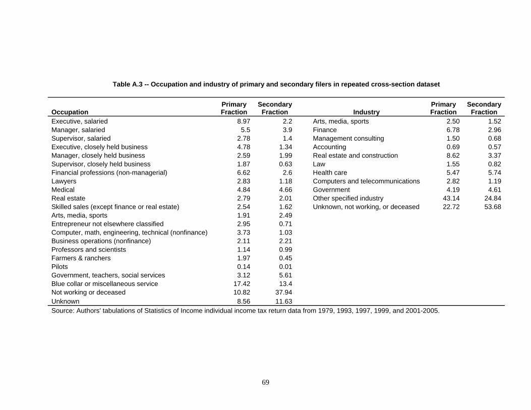
69
Table A.3 -- Occupation and industry of primary and secondary filers in repeated cross-section dataset
Occupation Primary Fraction
Secondary Fraction Industry
Primary Fraction
Secondary Fraction
Executive, salaried 8.97 2.2 Arts, media, sports 2.50 1.52 Manager, salaried 5.5 3.9 Finance 6.78 2.96 Supervisor, salaried 2.78 1.4 Management consulting 1.50 0.68 Executive, closely held business 4.78 1.34 Accounting 0.69 0.57 Manager, closely held business 2.59 1.99 Real estate and construction 8.62 3.37 Supervisor, closely held business 1.87 0.63 Law 1.55 0.82 Financial professions (non-managerial) 6.62 2.6 Health care 5.47 5.74 Lawyers 2.83 1.18 Computers and telecommunications 2.82 1.19 Medical 4.84 4.66 Government 4.19 4.61 Real estate 2.79 2.01 Other specified industry 43.14 24.84 Skilled sales (except finance or real estate) 2.54 1.62 Unknown, not working, or deceased 22.72 53.68 Arts, media, sports 1.91 2.49 Entrepreneur not elsewhere classified 2.95 0.71 Computer, math, engineering, technical (nonfinance) 3.73 1.03 Business operations (nonfinance) 2.11 2.21 Professors and scientists 1.14 0.99 Farmers & ranchers 1.97 0.45 Pilots 0.14 0.01 Government, teachers, social services 3.12 5.61 Blue collar or miscellaneous service 17.42 13.4 Not working or deceased 10.82 37.94 Unknown 8.56 11.63 Source: Authors' tabulations of Statistics of Income individual income tax return data from 1979, 1993, 1997, 1999, and 2001-2005.

70
Table A.4 -- Sample statistics from 1987-2005 panel of tax returns, sample used for estimation
Mean St. Dev. ln(Net ot Tax Share) -0.499 0.123Income Excluding Capital Gains 1,174,150 5,253,504 Age 46.583 9.331Male 0.900 0.300Married 0.805 0.396Children at Home 0.496 0.805Other Dependents 0.719 1.103 Executive 0.150 0.357Manager 0.131 0.337Supervisor 0.089 0.285Finance 0.106 0.308Lawyer 0.060 0.237Real Estate 0.020 0.140Skilled sales 0.057 0.233Media and Sports 0.033 0.178Entrepreneur 0.029 0.169Technical 0.096 0.294Professors and Scientists 0.046 0.210 ln(House Price) 11.933 0.377ln(Real S&P 500) 6.644 0.361State Unemployment Rate 0.060 0.014 Observations 244,909
Source: Authors' tabulations of Statistics of Income individual income tax return data from 1987-96 Family Panel, 1997-98 CWHS Returns, and 1999-2005 Edited Panel.

71
Table A.5 -- Income Characteristics of Panel Estimation Sample
Fraction of
sample Number of
observations
Minimum income (excluding capital gains) in
2005, in thousands of constant year 2007 dollars
Below 90th percenitle of national income distribution 0.30 72,569 10 90th to 95th percentiles 0.10 25,438 94 95th to 99th percentiles 0.18 43,733 129 99th to 99.5th percentiles 0.06 15,787 295 99.5th to 99.9th percentiles 0.15 37,255 450 Top 0.1 percent 0.20 50,127 1,246

72
Figure 1 -- Percentage of national income (excluding capital gains) received by top 0.1% of income earners: United States, France, and Japan, 1981 - 2006
0
1
2
3
4
5
6
7
8
9
1981 1985 1989 1993 1997 2001 2005
Year
Top
0.1%
Inco
me
Shar
e, P
erce
nt
U.S.
France
Japan
Source: Piketty and Saez (2003, updated in 2008 at <http://elsa.berkeley.edu/~saez/TabFig2006.xls>; Moriguchi and Saez (2008); Piketty (2003); Landais (2008); and upublished tables provided to the authors by Camille Landais.

73
Figure 2 -- Top marginal income tax rate: United States, France, and Japan, 1981 - 2006
0
10
20
30
40
50
60
70
80
1981 1985 1989 1993 1997 2001 2005
Year
Mar
gina
l Tax
Rat
e, P
erce
nt
U.S.
France
Japan
Source: OECD (2009).

74
Figure 3 -- Index of average stock prices, adjusted for inflation: United States, France, and Japan, 1981 - 2006
0
100
200
300
400
500
600
700
800
1981 1985 1989 1993 1997 2001 2005
Year
Stoc
k pr
ice
inde
x (=
100
in 1
981)
U.S.
France
Japan
Source: OECD (2009). Depicts the NYSE Composite index for the U.S., the TSE Topix All Shares index for Japan, and the Paris Stock Exchange SBF 250 index for France, each deflated using each country's consumer price index.

75
Figure 4 -- Mean income excluding capital gains in thousands of constant year 2007 dollars, top 1% but outside top 0.5% of distribution, by job of primary taxpayer, using constant 1979
job shares
0
50
100
150
200
250
300
1979 1984 1989 1994 1999 2004
Year
Inco
me,
thou
sand
s of
$
FinanceReal EstateExecutivesLawyersMedicalManagers

76
Figure 5 -- Mean income excluding capital gains in thousands of constant year 2007 dollars, top 0.5% but outside 0.1% of distribution, by job of primary taxpayer, using constant 1979 job
shares
0
100
200
300
400
500
600
700
800
900
1,000
1979 1984 1989 1994 1999 2004
Year
Inco
me,
thou
sand
s of
$
FinanceReal EstateExecutivesLawyersMedicalManagers

77
Figure 6 -- Mean income excluding capital gains in thousands of constant year 2007 dollars, top 0.1% of distribution, by job of primary taxpayer, using constant 1979 job shares
0
1,000
2,000
3,000
4,000
5,000
6,000
1979 1984 1989 1994 1999 2004
Year
Inco
me,
thou
sand
s of
$
FinanceReal EstateExecutivesLawyersMedicalManagers


