FINAL REPORT –
Improved Data & Tools
for Integrated Land
Use-Transportation
Planning in California
Raef Porter, Sacramento Area Council of Governments (SACOG)
August 6, 2012
APPENDIX G
VMT Spreadsheet Tool
TOPICS:
1. Overview of Tool
2. Code Documentation
3. User Guide
4. Validation Test Plan and
Results

Improved Data and Tools for Integrated Land Use-Transportation Planning in California
Appendix G – Spreadsheet Tool: Documentation, User Guide, and Testing 2
Table of Contents
1. Overview of Spreadsheet Tool
A. Overview ...............……….……….3
2. Code Documentation
A. Silverlight Web GIS……………….3
3. User Guide
A. Sketch7 ………………..….............4
B. Silverlight Web GIS …......……..11
4. Validation Test Plan and Results
A. Calculation Accuracy …............16
B. Reasonableness .......................16

Improved Data and Tools for Integrated Land Use-Transportation Planning in California
Appendix G – Spreadsheet Tool: Documentation, User Guide, and Testing 3
1. Overview of VMT Spreadsheet Tool
The VMT spreadsheet tool is intended to give the user a sketch level comparison of different land
use and transportation scenarios. It conducts a sketch level analysis of the land use and
transportation relationships using 7 Ds: density, diversity, distance, design, destination,
demographics, and development scale. It looks at how a land use scenario differs from an
established or modeled land use scenario, comparing the two on land use metrics like number and
types of jobs and households, densities, and the mix of uses. The tool also compares the scenarios
on travel behavior, and - depending on the scale of the project - can provide estimates of vehicle
miles traveled (VMT).
In the regional context, the tool provides VMT estimates that can be useful in scenario planning
and evaluation. The project level evaluation compares land use variables as a “sketch” of whether
an alternative scenario may perform better or worse than a base scenario. This level of use is not
intended to replace the type of analysis better suited for more robust travel models or analysis
tools, but to provide planners, developers, analysts, and elected officials a way of quickly
comparing an alternative scenario to a base scenario.
The tool contains two parts. The main component of is a spreadsheet, Sketch7, built in Microsoft
Excel. This is where all of the calculations take place. The other part is a web based GIS application,
built in Microsoft Silverlight. The GIS portion is for making land use changes, and feeding the
spreadsheet the appropriate land use data.
The rest of this documentation outlines the steps necessary to install, calibrate, and use the VMT
spreadsheet tool.
2. Code Documentation
A. Silverlight Web GIS
A zip file with the custom GIS application, written in Silverlight, is available at
http://downloads.ice.ucdavis.edu/ultrans/statewidetools/StatewideToolsWebFiles.zip. The contents of
the file should be unzipped into a new folder. Visual Studio 2010 is required to open the project
by selecting the *.sln file. Once the project is opened, the solution explorer will reveal a web
section and a Silverlight section. All changes in the code should be performed in the Silverlight
portion of the site. Finally, the site will need to be published to a web server using Visual Studio.
To see an example of the application, please visit http://mapping.sacog.org/landusebuffer/.
Improved Data and Tools for Integrated Land Use-Transportation Planning in California
Appendix G – Spreadsheet Tool: Documentation, User Guide, and Testing 4
3. User Guide
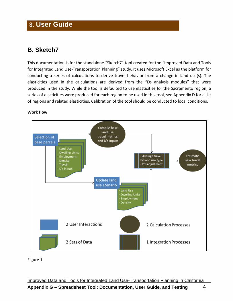
B. Sketch7
This documentation is for the standalone “Sketch7” tool created for the “Improved Data and Tools
for Integrated Land Use-Transportation Planning” study. It uses Microsoft Excel as the platform for
conducting a series of calculations to derive travel behavior from a change in land use(s). The
elasticities used in the calculations are derived from the “Ds analysis modules” that were
produced in the study. While the tool is defaulted to use elasticities for the Sacramento region, a
series of elasticities were produced for each region to be used in this tool, see Appendix D for a list
of regions and related elasticities. Calibration of the tool should be conducted to local conditions.
Work flow
Figure 1
Improved Data and Tools for Integrated Land Use-Transportation Planning in California
Appendix G – Spreadsheet Tool: Documentation, User Guide, and Testing 5
The figure above shows the flow of the process used in the estimation of travel based on a change
in land use in the Sketch7 land use-transportation standalone estimation tool. It begins with the
selection of a base set of parcels, the creation of a land use scenario, and estimation of final
metrics. Between each step, the tool conducts several calculations to create base and context area
averages for comparison purposes. The next sections of this document outline the steps within
Sketch7, organized by tabs within the spreadsheet.
start
There are three user actions or options on the start tab:
Project Name,
A button labeled “Map”, which opens the web based GIS application and allows the user to
enter the land use scenario, and
A button labeled “Import”, which allows the user to browse to the location of a saved
version of the mapped land use scenario.
There are also three buttons that take the user to a screen to enter base data:
Regional Land Use and Travel Data
Elasticities
Place Types
The user first enters the name of the project. The user then clicks on the Map button to open the
Silverlight GIS mapping application. Sketch7 opens a web browser for the Silverlight GIS mapping
tool, which allows the user to select parcels, buffer them ¼ mile, change land uses, and export the
new scenario to the spreadsheet tool (see prior documentation on this functionality). The
Silverlight GIS map sets the context area for the analysis by assigning a transportation analysis
zone (TAZ) to the project location. This TAZ becomes the base for all land use and travel metrics
that are then adjusted using the elasticities set in the tool.
Once a land use scenario is created, the tool computes two sets of data. The first set is the place
type average land use and travel metrics to be used for the base scenario and the newly created
scenario. This includes the following:
Totals by Place Types: Household Population, Households, Retail
Jobs, Non-Retail Jobs,
Improved Data and Tools for Integrated Land Use-Transportation Planning in California
Appendix G – Spreadsheet Tool: Documentation, User Guide, and Testing 6
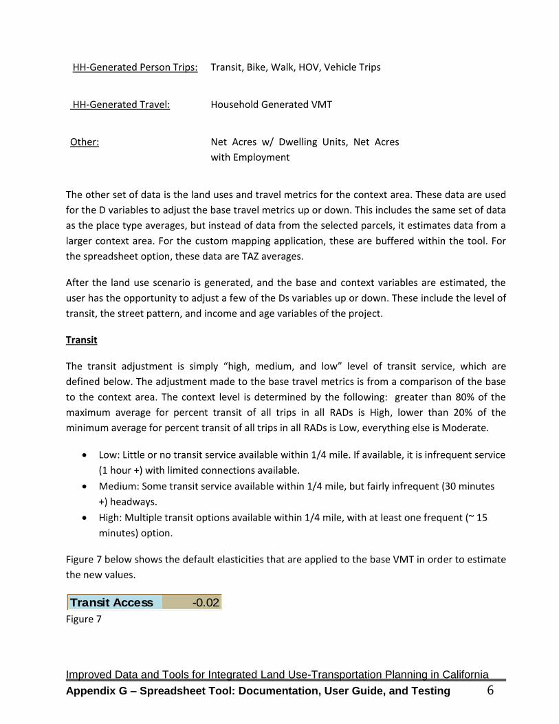
HH-Generated Person Trips: Transit, Bike, Walk, HOV, Vehicle Trips
HH-Generated Travel: Household Generated VMT
Other: Net Acres w/ Dwelling Units, Net Acres
with Employment
The other set of data is the land uses and travel metrics for the context area. These data are used
for the D variables to adjust the base travel metrics up or down. This includes the same set of data
as the place type averages, but instead of data from the selected parcels, it estimates data from a
larger context area. For the custom mapping application, these are buffered within the tool. For
the spreadsheet option, these data are TAZ averages.
After the land use scenario is generated, and the base and context variables are estimated, the
user has the opportunity to adjust a few of the Ds variables up or down. These include the level of
transit, the street pattern, and income and age variables of the project.
Transit
The transit adjustment is simply “high, medium, and low” level of transit service, which are
defined below. The adjustment made to the base travel metrics is from a comparison of the base
to the context area. The context level is determined by the following: greater than 80% of the
maximum average for percent transit of all trips in all RADs is High, lower than 20% of the
minimum average for percent transit of all trips in all RADs is Low, everything else is Moderate.
Low: Little or no transit service available within 1/4 mile. If available, it is infrequent service
(1 hour +) with limited connections available.
Medium: Some transit service available within 1/4 mile, but fairly infrequent (30 minutes
+) headways.
High: Multiple transit options available within 1/4 mile, with at least one frequent (~ 15
minutes) option.
Figure 7 below shows the default elasticities that are applied to the base VMT in order to estimate
the new values.
Figure 7
Transit Access -0.02

Improved Data and Tools for Integrated Land Use-Transportation Planning in California
Appendix G – Spreadsheet Tool: Documentation, User Guide, and Testing 7
Street
Similar to the adjustment for transit service, street connectivity or Design is set to Low, Moderate,
and High; see below for an explanation. These values are then compared to the context value,
which is determined by the following: greater than 80% of the maximum average for percent walk
and bike trips of all trips in all counties is High, lower than 20% of the minimum average for
percent walk and bike trips of all trips in all counties is Low, everything else is Moderate.
Cul-De-Sac style street design with limited 4-way intersections and large block faces.
Mixed Block style street design with some 4-way intersections and some smaller block
faces.
Grid style street design with many 4-way intersections and smaller block faces.
Figure 8
Figure 8 above shows the default elasticities prior to updates resulting from the land use project.
Demographics
There are two demographic variables that the user can set for the area, age and income. How the
variables are set for the project is described below.
Age: Income:
Fewer people 55 and older Fewer households above median income
Average amount of people 55 and older Households near median income
More people 55 and older More households above median income
Figure 9
Figure 9 above shows the default elasticities prior to updates resulting from the land use project.
Income -0.02
Age -0.01
Improved Data and Tools for Integrated Land Use-Transportation Planning in California
Appendix G – Spreadsheet Tool: Documentation, User Guide, and Testing 8
The other Ds variables are set by the location and the combination of land uses selected by the
user. These include: Destination (Accessibility), Density, Diversity, and Development Scale. These
are described below.
There are two types of accessibility measures: transit and auto accessibility. Transit accessibility is
defined by the number of jobs that can be reached with a 45 minute transit trip, and auto
accessibility is the number of jobs accessible within a 20 minute drive. The context is defaulted to
the RAD average, and the project adjusts that number up or down depending on the number of
jobs added to the scenario.
Figure 10 below shows the default elasticities for the Accessibility variables.
Figure 10
The Diversity adjustment is based on the difference between the context average for each specific
component: Retail Employee per Dwelling Unit, Total Jobs per Dwelling Unit, and K-12 Employees
per Dwelling Unit; and the optimal value in order to receive maximum travel benefit. Figure 11
shows the optimal value, and the elasticity used for each.
Figure 11
The Density adjustment is the gross density (jobs + dwelling units / gross acres) for the project
area compared to the context area. The base is adjusted up or down depending on whether
density in the project area increases density in the context area or not. The calculation is simply
project divided by context – 1.
Figure 12
Figure 12 above shows the elasticity for this variable.
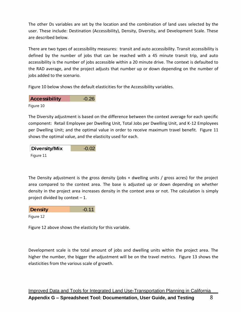
Development scale is the total amount of jobs and dwelling units within the project area. The
higher the number, the bigger the adjustment will be on the travel metrics. Figure 13 shows the
elasticities from the various scale of growth.
Accessibility -0.26
Diversity/Mix -0.02
Density -0.11
Improved Data and Tools for Integrated Land Use-Transportation Planning in California
Appendix G – Spreadsheet Tool: Documentation, User Guide, and Testing 9
Figure 13
Input
Once a user has created a land use scenario, adjusted Ds variables, and the tool has estimated
travel demand, the user can alter the land uses to either optimize the scenario or better reflect
observed results.
On this tab, the user simple adjusts the dwelling units, total employees, retail employees, and
non-retail employees. The tool will automatically adjust the travel metrics to reflect the changes in
land use.
These data are then compared to the TAZ averages calculated above to set the unadjusted land
use and travel metrics for the scenario. The next step is for the user to adjust the “Ds” variables to
estimate the change in travel.
The final report produced by this tool performs an assessment of each Ds variable for the project
as compared to the context area and the region. Based on this assessment, the base travel metrics
are adjusted up or down using the above-stated elasticities. The base travel metrics are shown
alongside the non-adjusted numbers for the project, as well as the final adjusted travel estimates.
Figure 14 below is an example of the tool’s final report.
Development Scale
Scale Adjustment
0 0
500 0
1000 0
2000 0
5000 0
15000 -0.00001
50000 -0.0001
200000 -0.001
1000000 -0.01

Improved Data and Tools for Integrated Land Use-Transportation Planning in California
Appendix G – Spreadsheet Tool: Documentation, User Guide, and Testing 10
Figure 24
Table 1. Assessment of Key Land Use and Travel Characteristics
RegionContext
Area
1,212 2,795
453 1,637
1.2 0.9
3.00 4.66
$60,000 $37,547
35 37
16.57 19.26
0.05 0.04
0.35 0.25
Table 2. Summary of Adjustments to Base Travel Metrics
Density Development Design Distance
Auto
Access
Transit
Access
J/H
BalanceRes. Mix
Res.
DensityIncome Age Scale
Street
Pattern
Transit
DistanceTOTAL
VMT per Capita -6.26% -4.79% 0.76% #DIV/0! 0.00% -0.20% 0.00% 0.00% -0.20% #DIV/0!
Transit Trips per Capita
B+W Trips per Capita
Table 3. Final Project VMT
Regional Context Area
Non-
Adjusted
Project
Adjusted
Project
VMT Per Capita 16.57 19.26 17.24 #DIV/0!
Total VMT (1000s) 36,699 560.4 75.2 #DIV/0!
Transit Trips per Capita
B+W Trips per Capita
B+W trips per capita
Transit Trips Per Capita
VMT per Capita
Age (Median
Householder Age)
Income (Median
income)
Residential Density
(Dwellings per Net Res
Acre, within a 0.5 mi
buffer)
4,249
1.4
Higher than average in
surrounding area, and
near regional average
Auto Accessibility
(Jobs w/in 20 Minute
Drive)
Residential Mix
(Entropy, 0.5 mile
buffer)
J/H Balance (Jobs per
Household w/in 4 miles)
Transit Accessibility
(Jobs w/in 45 Minute
Transit Trip)
Project Area Base
ValuesAssessment
#DIV/0!
Near average in
surrounding area, and
lower than regional
Near average in
surrounding area, and
near regional average
Near average in
surrounding area, and
near regional average
Lower median
householder age
More households below
median income
Destination Diversity Demographics
Higher than average in
surrounding area, and
higher than regional
Higher than average in
surrounding area, and
higher than regional
0.21
0.04
17.24
#DIV/0!
5,407
Start OverPrint

Improved Data and Tools for Integrated Land Use-Transportation Planning in California
Appendix G – Spreadsheet Tool: Documentation, User Guide, and Testing 11
In order for all calculations to take place, a set of land uses needs to be entered into the tool, and
base set of data from a regional travel model using the same land uses needs to be loaded.
place types
The land uses, or place types within Sketch7, are defaulted to a generic set of land uses used in
this study. The information that is needed within the place types tab includes:
Name Order (sorting order) Residential Density (dwellings per acre)
Employment Density (employees per acre) % Retail (% of land for retail uses)
The place types used in Sketch7 must be consistent with those used in the Silverlight GIS mapping
application as well as the travel model used to supply base metrics.
regional data
Regional data from a TAZ based travel model must be entered into the tool for each place type. By
TAZ and place type, these data are:
Household Population Dwelling Units Employees Retail Employees
Non-Retail Employees Acres w/ DUs Acres w/ Emps Total Trips
Vehicle Trips Walk Trips Bike Trips Transit Trips
VMT/HH VMT/Capita Jobs w/in 20 minute Drive
Jobs w/in 45 transit trip
B. Silverlight Web GIS
For the Sacramento region, the tool can be found by navigating to the following URL
http://mapping.sacog.org/landusebuffer. The purpose of the website is to enable a user to select
one or more parcel locations within the SACOG area on the map and produce a buffer from those
points to retrieve all parcels within that buffer. A table then appears showing data for each parcel
along with a highlighted selection of each parcels location. At this point the user can adjust the
original data to fit the needs of a particular scenario. The Employment, Dwelling Units, and
Landuse Type fields are all editable and can be changed to any value the user desires. Lastly,
when all field value changes are completed the user can export the table into an xml spreadsheet
onto their local computer to export into an Excel spreadsheet for further analysis.
Web server administrators have a few requirements to fulfill to host the application. The website
utilizes ESRI’s ArcServer GIS web mapping technology with data stored in an ArcSDE database for
use over the internet. Data storage can also include shapefiles and file based geodatabases. A

Improved Data and Tools for Integrated Land Use-Transportation Planning in California
Appendix G – Spreadsheet Tool: Documentation, User Guide, and Testing 12
copy of Microsoft Visual Studio will be needed to change URL parameters and publishing of the
website onto an IIS based web server. Users of the website also have the requirement of installing
the Microsoft Silverlight browser plugin before they can view the web site. Upon navigating the
site, a script checks to see if the browser contains the plugin, and if not provides a link to install.
The shapefile or geodatabase must include the following fields:
Landuse Type (must be consistent with the place types in Sketch7)
Dwelling Units
Employees
TAZ
The initial screen shows a map view of the Curtis Park area in Sacramento, CA and various
elements including a toolbar, map navigation tool, scalebar, and an overview map. The map is
navigable in a similar fashion to Google or Bing maps. The scroll button zooms in and out while
click and dragging pans the map view. The navigation tool at the lower left section of the web site
allows the user to perform the same actions as using mouse activities. The overview window
shows the current map extent using a red outlined box and the surrounding area. Clicking and
dragging the red box will pan the window to that location. The bottom center of the screen
displays a scalebar that adjusts itself when zooming in or out.
A toolbar containing three tools appears at the top right corner of the website. A user will select
the point tool in order to select a parcel that will be used in buffering. It is recommended that an
actual parcel be selected otherwise a message will appear explaining a parcel does not exist at
that location. This point then becomes the location where the buffer will originate. If another
point is desired in the overall selection, then the user will have to select the point tool again and
place a second point on the screen. This process can be repeated for as many points on the map
as desired. When all points are placed on the map, the Buffer Parcels button is selected and the
buffer will take place. A table will appear on the upper left corner of the screen showing all
parcels that were selected in the buffer. The selected parcels will also appear highlighted in blue
on the map. When hovering the mouse over each record in the table, it will highlight to a cyan
color as well as highlight the parcel that corresponds to that record on the map. This will help the
user identify which record corresponds with the desired parcel. The table is now available for
attributes to be edited. A permanent change to the underlying database is not being performed,
changes will only be noted when the table is exported. After all changes are made to the scenario,
the user will click the Save Results button on the table and export to an xml file onto their local
desktop. This file will then be used in the next step of the process. If an undesirable buffer was

Improved Data and Tools for Integrated Land Use-Transportation Planning in California
Appendix G – Spreadsheet Tool: Documentation, User Guide, and Testing 13
performed or the user wishes to experiment with various buffers, the Clear Tool must be selected
to reset the table and graphics in order to perform new buffers.
Navigation
Upon navigating to the website located at http://mapping.sacog.org/landusebuffer, a map
appears showing the extent of the SACOG region. The map interacts similar to a Google map in
that panning and zooming are controlled by the mouse and mouse wheel. An additional zoom
tool exists as well by pressing the shift key and drawing a rectangle on the screen to zoom into the
desired area. A navigation control is also available in the upper left corner of the map that
interacts similar to Google maps.
Figure 3
Toolbar
The toolbar consists of 4 tools that include parcel selection, clear, buffer, and display help,
respectively.
Figure 4
Parcel Selection = When zoomed in within a close enough scale, parcels will display on the
screen. The user will click the parcel selection tool and begin to select parcels on the screen
whose values will then be changed later in a table for the simulation. Once the tool is initiated, as
many parcels as desired will be selected.

Improved Data and Tools for Integrated Land Use-Transportation Planning in California
Appendix G – Spreadsheet Tool: Documentation, User Guide, and Testing 14
Clear = Clears all graphics and resets parcel selections from the screen. Useful if a parcel
selection needs to be reselected to achieve a different buffer area.
Buffer = Once parcels are selected on the map, a buffer of 0.5 mile will be performed and
all parcels within that buffer will become selected and highlighted on the map. A table will then
appear in the lower left screen showing the parcel(s) selected before the buffer occurred. These
values can then be edited directly in the table.
Help = Displays the help.
Basic Workflow – Below describes a basic workflow using the above tools
Zoom to desired area
Select parcel selection tool
Select parcel(s)
Figure 5
Click the Buffer button

Improved Data and Tools for Integrated Land Use-Transportation Planning in California
Appendix G – Spreadsheet Tool: Documentation, User Guide, and Testing 15
Figure 6
Edit values in the table
Figure 7
Click the Save Results button to save the edited records in the table and the buffered surrounding
parcels to an excel file.
4. Validation Test Plan and Results
In order to test the effectiveness of the tool, several tests were conducted. These are:
• Testing the accuracy of the calculations
• Testing the reasonableness of the results
Improved Data and Tools for Integrated Land Use-Transportation Planning in California
Appendix G – Spreadsheet Tool: Documentation, User Guide, and Testing 16
These tests area appropriate levels of testing for sketch tools, which are not intended to provide
specific numbers to be used in more rigorous evaluations, but rather to give users a sense of
magnitude and direction between different planning scenarios.
A. Calculation Accuracy
The calculation tests are a simple way to check if the tool is functioning in the way it is intended. It
is not meant to determine if results are accurate, just whether the calculations in the tool are
working appropriately. A simple test would be seeing if 1 + 1 in the tool equals 2.
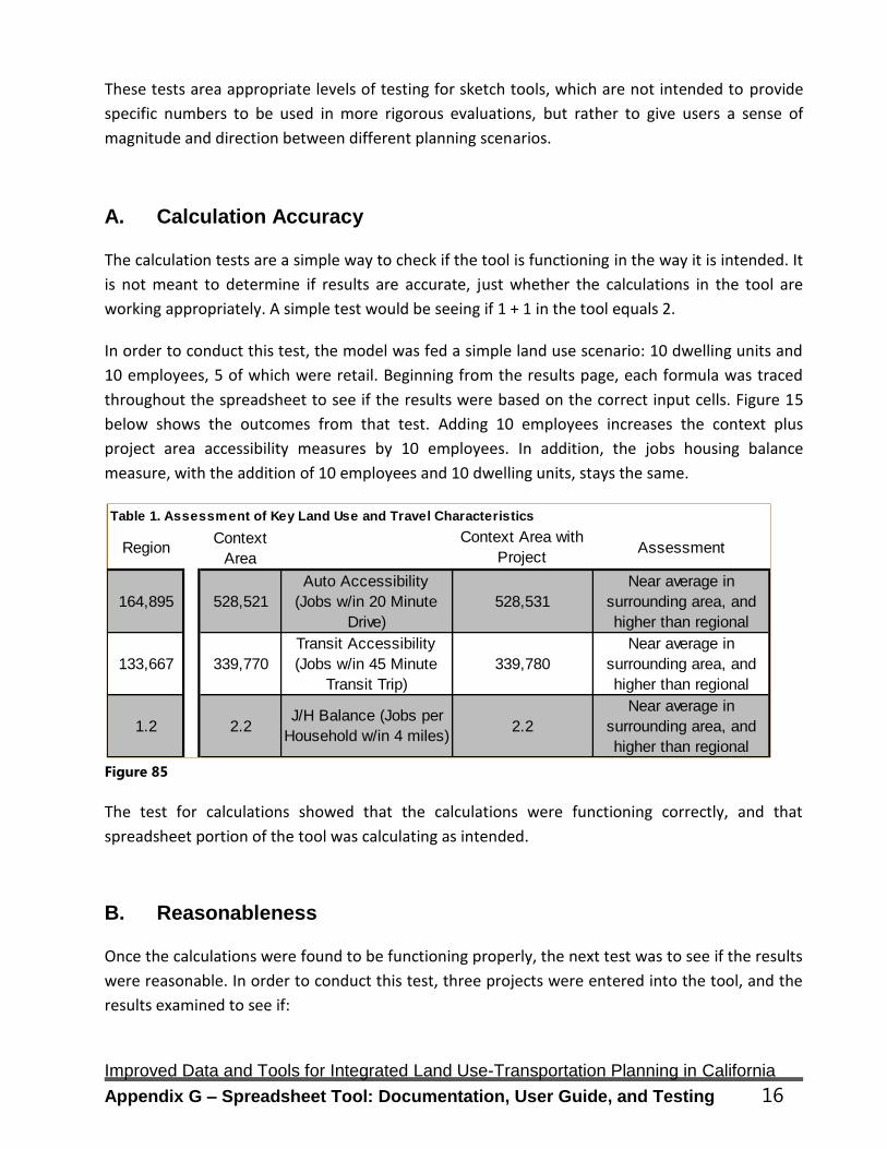
In order to conduct this test, the model was fed a simple land use scenario: 10 dwelling units and
10 employees, 5 of which were retail. Beginning from the results page, each formula was traced
throughout the spreadsheet to see if the results were based on the correct input cells. Figure 15
below shows the outcomes from that test. Adding 10 employees increases the context plus
project area accessibility measures by 10 employees. In addition, the jobs housing balance
measure, with the addition of 10 employees and 10 dwelling units, stays the same.
Figure 85
The test for calculations showed that the calculations were functioning correctly, and that
spreadsheet portion of the tool was calculating as intended.
B. Reasonableness
Once the calculations were found to be functioning properly, the next test was to see if the results
were reasonable. In order to conduct this test, three projects were entered into the tool, and the
results examined to see if:
Table 1. Assessment of Key Land Use and Travel Characteristics
RegionContext
Area
164,895 528,521
133,667 339,770
1.2 2.2
339,780
2.2
Near average in
surrounding area, and
higher than regional
Auto Accessibility
(Jobs w/in 20 Minute
Drive)
J/H Balance (Jobs per
Household w/in 4 miles)
Transit Accessibility
(Jobs w/in 45 Minute
Transit Trip)
Context Area with
ProjectAssessment
Near average in
surrounding area, and
higher than regional
Near average in
surrounding area, and
higher than regional
528,531

Improved Data and Tools for Integrated Land Use-Transportation Planning in California
Appendix G – Spreadsheet Tool: Documentation, User Guide, and Testing 17
1. Estimated VMT was not higher or lower than expected,
2. Estimated mode shares were not higher or lower than expected, and
3. Given the land uses, the Ds variables and the adjustments they were making to the
base VMT made sense.
The three projects tested were: Curtis Park Village in the city of Sacramento, La Valentina in
Downtown Sacramento, and a non-geographically specific low density neighborhood.
Curtis Park Village was selected as SACOG had conducted analysis for the city of Sacramento and
the Sacramento Air Quality Management District on this project. The project version evaluated
contains approximately 530 dwelling units and 450 employees over 95 acres. The context area for
the project is a typical inner-ring suburb in Sacramento with an abundance of mostly retail jobs,
and medium density residential that is well-served by transit. The project is proposing a mix of
uses, with slightly more residential units at a higher density. One portion of the project is designed
for senior housing.
The test of the tool resulted in a VMT/HH of 44.3. SACOG’s evaluation of the project using its
SACSIM activity-based travel demand model resulted in a VMT/HH of 44.5, a difference of less
than 1 percent. The share of trips resulted in increases in all non-auto modes from the regional
average, including a 4% increase in walk/bike trips and a 4.4% increase in transit trips. Given the
context area around the project, the existing and proposed demographics, and the proposed uses
on the site, these slight increases aligned with our expectations.
La Valentina is an urban project that consists of two parcels totaling just over 1 acre in size. The
proposed project used in this analysis is a mixed-use development that consists of 81 dwelling
units and 30 jobs, 15 of which are retail. The context area immediately surrounding the project is
urban, with an abundance of jobs, retail jobs, and fewer dwelling units, most of which are of
medium to medium-high density.
The test of the tool resulted in a VMT per capita of 11.3, which seemed reasonable for an urban
mixed-use project. A SACSIM analysis of the surrounding ½ mile area resulted in an average VMT
per capita of 13.4. While this is 15% higher, given the mixed land uses and improved jobs-to-
housing ratio with the addition of more housing, it makes sense to see an improvement over the
surrounding area.
In order to find out if the improvements to the project warranted a 15% decrease in per capita
VMT, the project was changed to reflect the typical development found in the area. The two
parcels were set to medium-high density residential with no employment. As shown in Figure 16,
this resulted in a VMT per capita almost identical to the context area.

Improved Data and Tools for Integrated Land Use-Transportation Planning in California
Appendix G – Spreadsheet Tool: Documentation, User Guide, and Testing 18
Figure 16
For sketch level planning, the results of the two scenarios are reasonable and trend in direction
that is expected. Although the models created for this tool are not intended to be used at this
small scale, SACOG will continue to work on calibrating the tool to reflect travel at this level.
The Low Density Neighborhood scenario was created to reflect a standard suburban
neighborhood that could occur anywhere. These areas typically are not served by transit, are not
accessible to many jobs in a short drive, and are fairly homogenous in land use characteristics. For
this test the project consisted of 100 single family dwelling units of approximately 4 dwelling units
per acre. For this test, the VMT per capita was 35.6. Given the characteristics of the land use and
lack of transit and accessibility to jobs, it seems reasonable the VMT per capita would be this high.
An additional test was done, setting the design, destination, and transit variables to those near the
regional average. For this test, the per capita VMT was 27.5, which is still 19% above regional
average. However, given that the project contained no employment and was at a slightly lower
density than the regional average, it seems reasonable that the per capita VMT would remain
slightly higher than the regional average.
Scenario
Res
VMT/
Capita
La Valentina 13.5
Base 23.1
Context Area Avg: 13.4


