
Approximate models for Physically Based Rendering - Siggraph 2015 Course: Physically Based Shading in Theory and Practice
Approximate models for
physically based rendering
Michał Iwanicki
Angelo Pesce
Activision
Approximate models for Physically Based Rendering - Siggraph 2015 Course: Physically Based Shading in Theory and Practice
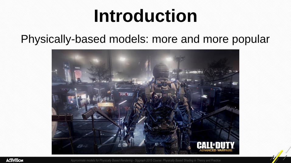
Introduction
Physically-based models: more and more popular

Approximate models for Physically Based Rendering - Siggraph 2015 Course: Physically Based Shading in Theory and Practice
Introduction
• Complex!
– No closed form solutions
– Real time applications can often afford only
the simplest cases
Approximate models for Physically Based Rendering - Siggraph 2015 Course: Physically Based Shading in Theory and Practice
Introduction
• How can we use them in real time?
• Model and approximate!
– Looks just as good (*)
– Way cheaper at runtime
(*) well, ok, almost ;-)
Approximate models for Physically Based Rendering - Siggraph 2015 Course: Physically Based Shading in Theory and Practice
Introduction
• Creating approximate models
– Trial-and-error process
– Practice makes perfect
• Sharing our experience
– Basic guidelines (*)
– Case studies!
(*) No worries, there’s more theory in the course notes
Approximate models for Physically Based Rendering - Siggraph 2015 Course: Physically Based Shading in Theory and Practice
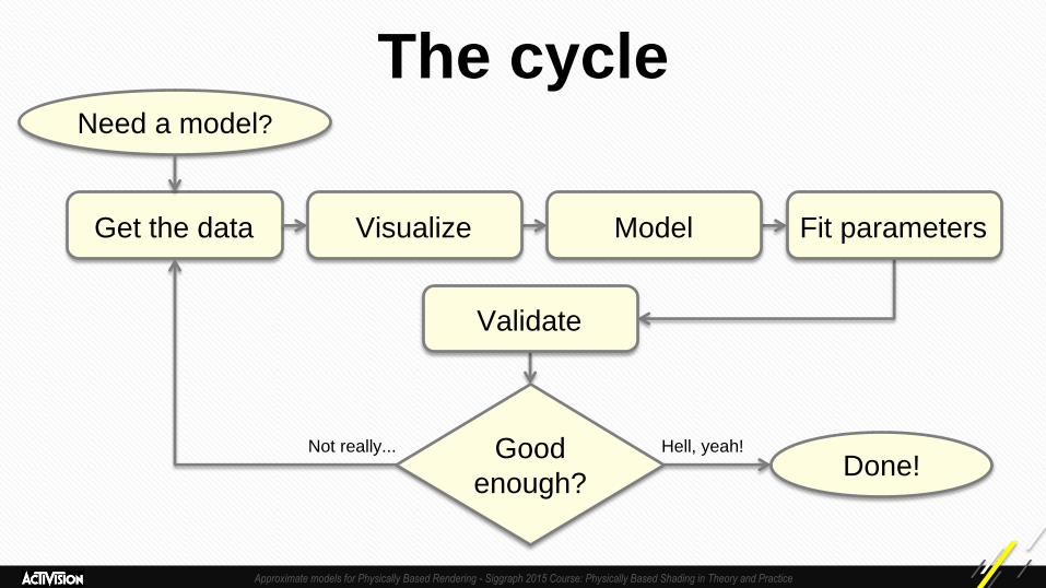
The cycle
Get the data
Not really... Hell, yeah!
Need a model?
Visualize Model Fit parameters
Validate
Good
enough? Done!
Approximate models for Physically Based Rendering - Siggraph 2015 Course: Physically Based Shading in Theory and Practice
1. Acquire the data
• From an existing model:
– E.g. compute the value of the BRDF for every
possible combination of input parameters
– E.g. compute the desired values using costly
precomputations
• From reality:
– Scan/measure
Approximate models for Physically Based Rendering - Siggraph 2015 Course: Physically Based Shading in Theory and Practice
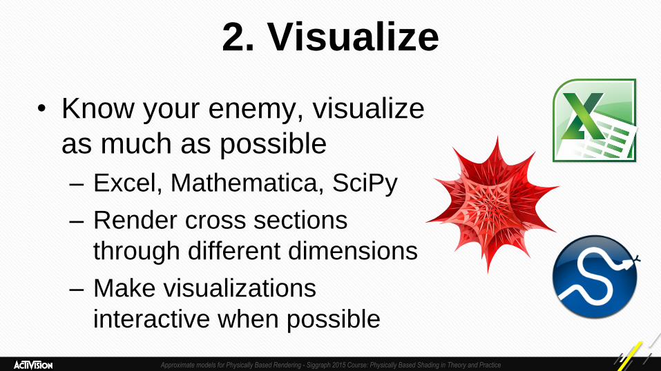
2. Visualize
• Know your enemy, visualize
as much as possible
– Excel, Mathematica, SciPy
– Render cross sections
through different dimensions
– Make visualizations
interactive when possible
Approximate models for Physically Based Rendering - Siggraph 2015 Course: Physically Based Shading in Theory and Practice
3. Create the approximate model
• The tricky part :)
• Start from visualized data
• Cheat sheet
Approximate models for Physically Based Rendering - Siggraph 2015 Course: Physically Based Shading in Theory and Practice
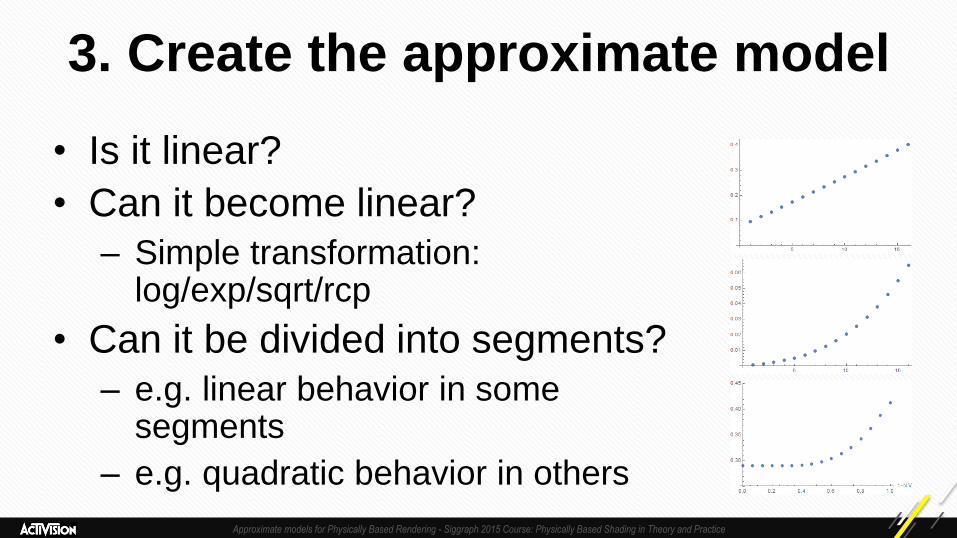
3. Create the approximate model
• Is it linear?
• Can it become linear?
– Simple transformation: log/exp/sqrt/rcp
• Can it be divided into segments?
– e.g. linear behavior in some segments
– e.g. quadratic behavior in others

Approximate models for Physically Based Rendering - Siggraph 2015 Course: Physically Based Shading in Theory and Practice
3. Create the approximate model
• Can we do dimensionality reduction
– e.g. if the function is radially symmetric
• Does it sweep between two behaviors?
– i.e. lerp(f(x),g(x),y)
– Does it sweep non-linearly?
Approximate models for Physically Based Rendering - Siggraph 2015 Course: Physically Based Shading in Theory and Practice
3. Create the approximate model
• If nothing simple comes out, try formulating
the model in terms of different variables
– Try combining terms
– Try expressing some terms as combinations
of others
• Careful with the number of free variables!
Approximate models for Physically Based Rendering - Siggraph 2015 Course: Physically Based Shading in Theory and Practice
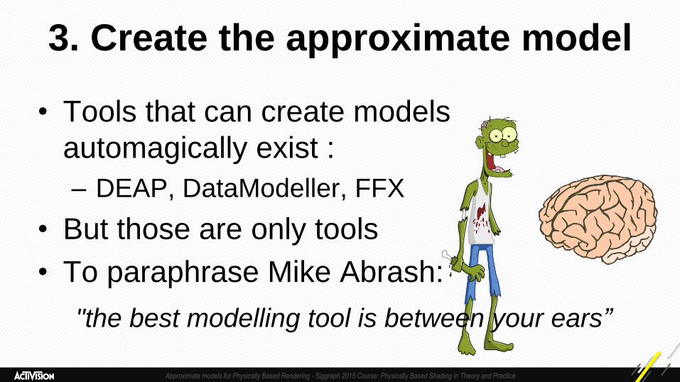
3. Create the approximate model
• Tools that can create models
automagically exist :
– DEAP, DataModeller, FFX
• But those are only tools
• To paraphrase Mike Abrash:
"the best modelling tool is between your ears”
Approximate models for Physically Based Rendering - Siggraph 2015 Course: Physically Based Shading in Theory and Practice
4. Fit Parameters to your model
• Your model needs parameters
• Optimizer for every occasion:
• Linear regression
• Local: – Gradient descent
– BFGS/L-BFGS
– Levenberg-Marquardt
– E-M
– Nelder-Mead Simplex
• Constrained/unconstrained
• Global: – Differential evolution
– Simulated annealing
– Multistart
Approximate models for Physically Based Rendering - Siggraph 2015 Course: Physically Based Shading in Theory and Practice
5. Check against ground truth
• Check the model in practice, not just on the plots!
• Lowest error doesn’t always mean the best result
– Finding the right metric might be tricky itself!
• Flip between your approximation and reference
• Automate as much as possible
• Collect all results
• Ensure they are reproducible

Approximate models for Physically Based Rendering - Siggraph 2015 Course: Physically Based Shading in Theory and Practice
Time for practice! There’s more in the course notes!
Approximate models for Physically Based Rendering - Siggraph 2015 Course: Physically Based Shading in Theory and Practice
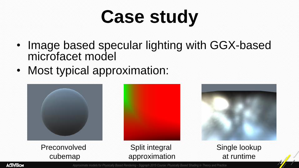
Case study
• Image based specular lighting with GGX-based microfacet model
• Most typical approximation:
Preconvolved
cubemap
Split integral
approximation
Single lookup
at runtime

Approximate models for Physically Based Rendering - Siggraph 2015 Course: Physically Based Shading in Theory and Practice
Issues with the current approach
• Preconvolving with symmetric kernel = no
elongated highlights
!=
Approximate models for Physically Based Rendering - Siggraph 2015 Course: Physically Based Shading in Theory and Practice
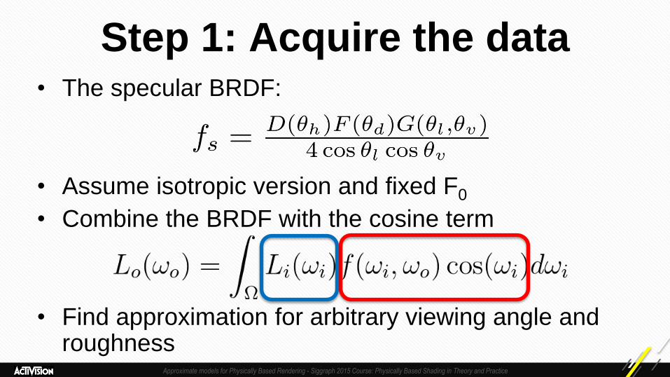
Step 1: Acquire the data • The specular BRDF:
• Assume isotropic version and fixed F0
• Combine the BRDF with the cosine term
• Find approximation for arbitrary viewing angle and roughness
Approximate models for Physically Based Rendering - Siggraph 2015 Course: Physically Based Shading in Theory and Practice
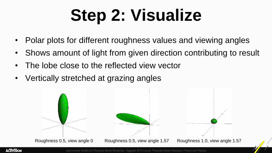
Step 2: Visualize
• Polar plots for different roughness values and viewing angles
• Shows amount of light from given direction contributing to result
• The lobe close to the reflected view vector
• Vertically stretched at grazing angles
Roughness 0.5, view angle 0 Roughness 0.5, view angle 1.57 Roughness 1.0, view angle 1.57
Approximate models for Physically Based Rendering - Siggraph 2015 Course: Physically Based Shading in Theory and Practice
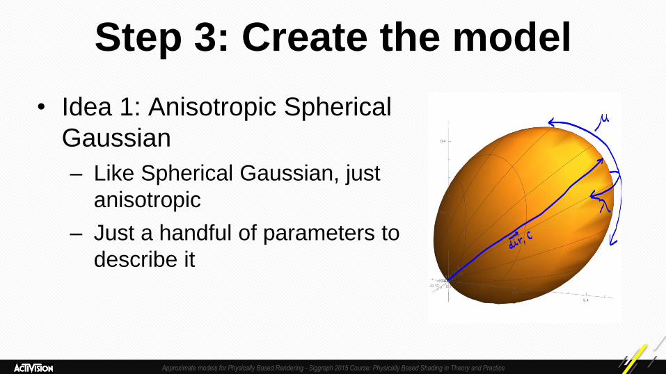
Step 3: Create the model
• Idea 1: Anisotropic Spherical
Gaussian
– Like Spherical Gaussian, just
anisotropic
– Just a handful of parameters to
describe it
Approximate models for Physically Based Rendering - Siggraph 2015 Course: Physically Based Shading in Theory and Practice
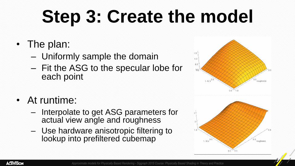
Step 3: Create the model
• The plan: – Uniformly sample the domain
– Fit the ASG to the specular lobe for each point
• At runtime: – Interpolate to get ASG parameters for
actual view angle and roughness
– Use hardware anisotropic filtering to lookup into prefiltered cubemap
Approximate models for Physically Based Rendering - Siggraph 2015 Course: Physically Based Shading in Theory and Practice
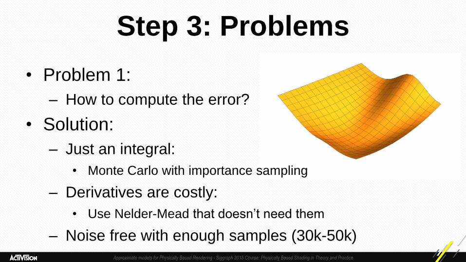
Step 3: Problems
• Problem 1:
– How to compute the error?
• Solution:
– Just an integral:
• Monte Carlo with importance sampling
– Derivatives are costly:
• Use Nelder-Mead that doesn’t need them
– Noise free with enough samples (30k-50k)
Approximate models for Physically Based Rendering - Siggraph 2015 Course: Physically Based Shading in Theory and Practice
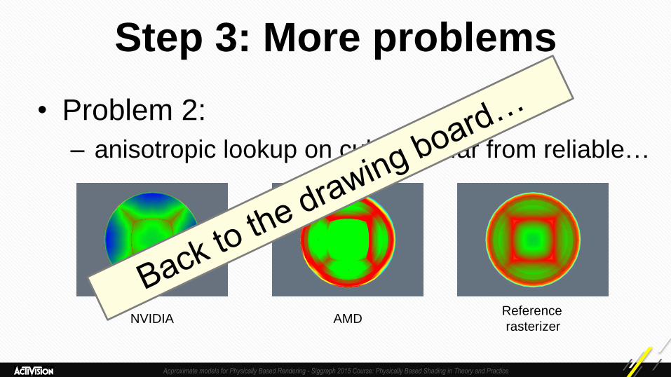
Step 3: More problems
• Problem 2:
– anisotropic lookup on cubemap far from reliable…
NVIDIA AMD Reference
rasterizer
Approximate models for Physically Based Rendering - Siggraph 2015 Course: Physically Based Shading in Theory and Practice
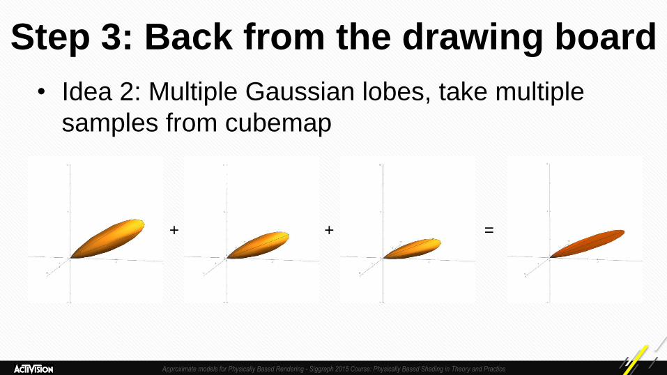
Step 3: Back from the drawing board
• Idea 2: Multiple Gaussian lobes, take multiple
samples from cubemap
+ + =
Approximate models for Physically Based Rendering - Siggraph 2015 Course: Physically Based Shading in Theory and Practice
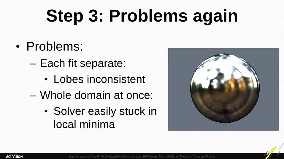
Step 3: Problems again
• Problems:
– Each fit separate:
• Lobes inconsistent
– Whole domain at once:
• Solver easily stuck in
local minima
Approximate models for Physically Based Rendering - Siggraph 2015 Course: Physically Based Shading in Theory and Practice
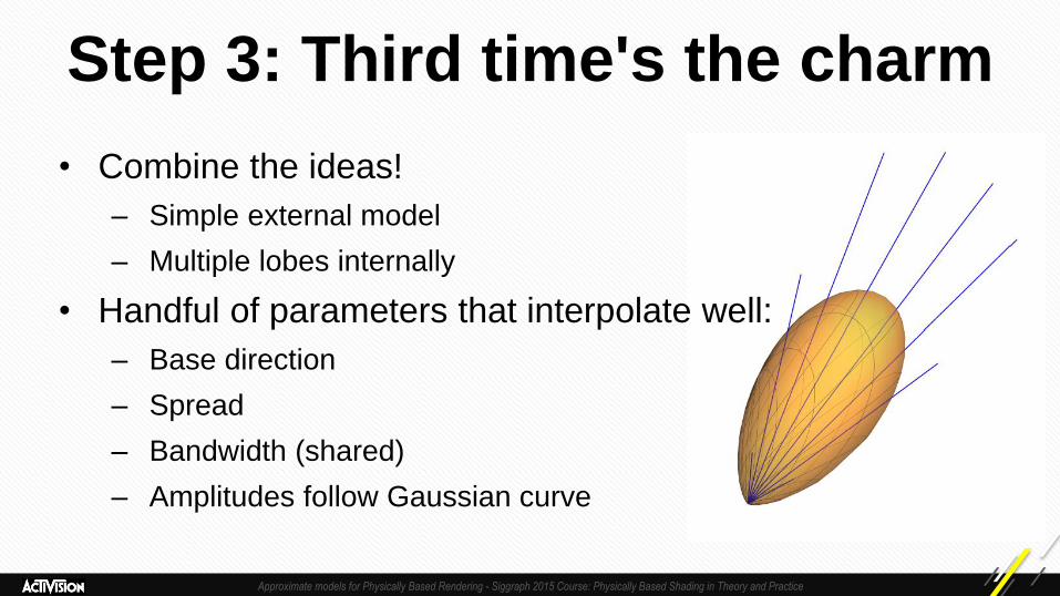
• Combine the ideas!
– Simple external model
– Multiple lobes internally
• Handful of parameters that interpolate well:
– Base direction
– Spread
– Bandwidth (shared)
– Amplitudes follow Gaussian curve
Step 3: Third time's the charm
Approximate models for Physically Based Rendering - Siggraph 2015 Course: Physically Based Shading in Theory and Practice
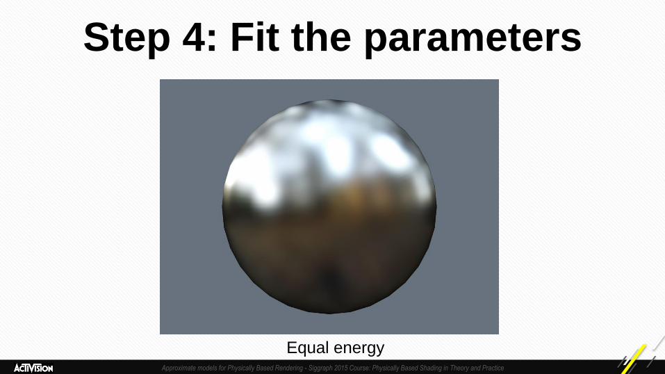
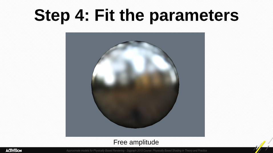
Step 4: Fit the parameters
• Nelder-Mead fit for every view angle and
roughness combination
• Local algorithm – it needs a good starting point:
– Generate near the expected solution
– Scan the domain and pick points with low error
Approximate models for Physically Based Rendering - Siggraph 2015 Course: Physically Based Shading in Theory and Practice
Step 4: Fit the parameters
• Fit values for roughness x view angle domain
– Each data point independent
– Each starting point independent
• Parallelize!
• Two variants:
– Amplitude forced to generate equal energy as GGX
– Amplitude as free variable
Approximate models for Physically Based Rendering - Siggraph 2015 Course: Physically Based Shading in Theory and Practice
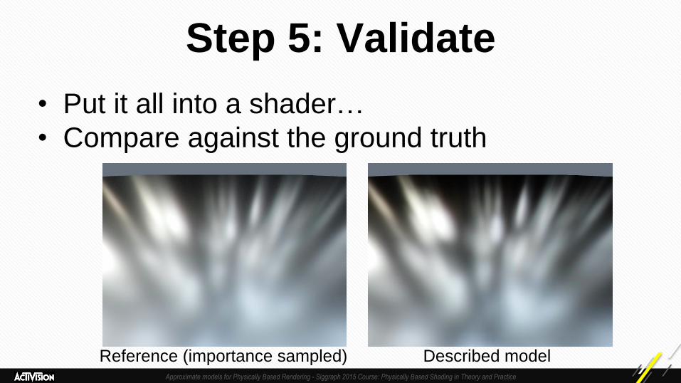
Step 5: Validate
• Put it all into a shader…
• Compare against the ground truth
Reference (importance sampled) Described model
Approximate models for Physically Based Rendering - Siggraph 2015 Course: Physically Based Shading in Theory and Practice
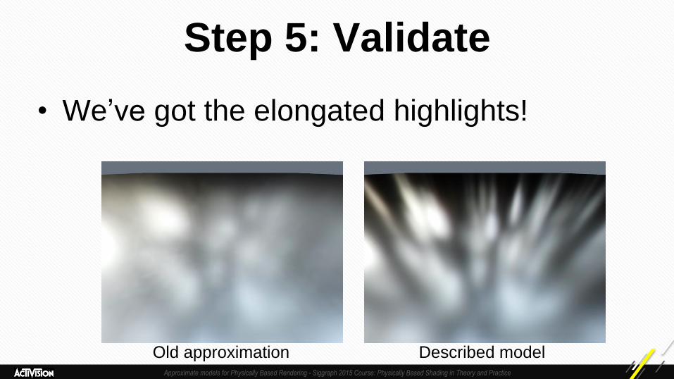
Step 5: Validate
• We’ve got the elongated highlights!
Old approximation Described model
Approximate models for Physically Based Rendering - Siggraph 2015 Course: Physically Based Shading in Theory and Practice
Step 4: Fit the parameters
Equal energy
Approximate models for Physically Based Rendering - Siggraph 2015 Course: Physically Based Shading in Theory and Practice
Step 4: Fit the parameters
Free amplitude

Approximate models for Physically Based Rendering - Siggraph 2015 Course: Physically Based Shading in Theory and Practice
Step 5: Validate more
• What happens at high
roughness?
• When spread > θ we
get radial artifacts
• Damn, so close...
Approximate models for Physically Based Rendering - Siggraph 2015 Course: Physically Based Shading in Theory and Practice
Corrections to the model
• Add a constraint, make sure that spread is no
larger than θ
• Super simple with Nelder-Mead:
– Penalty term
– Trivial changes to the algorithm itself
• Not entirely kosher, but works just fine in practice

Approximate models for Physically Based Rendering - Siggraph 2015 Course: Physically Based Shading in Theory and Practice
Step 5.1: Validate again
• Much better
Approximate models for Physically Based Rendering - Siggraph 2015 Course: Physically Based Shading in Theory and Practice
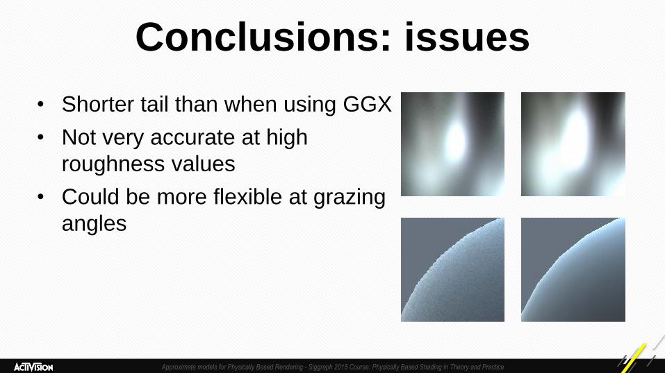
Conclusions: issues
• Shorter tail than when using GGX
• Not very accurate at high
roughness values
• Could be more flexible at grazing
angles
Approximate models for Physically Based Rendering - Siggraph 2015 Course: Physically Based Shading in Theory and Practice
Conclusions
• What’s next?
– Different number of lobes for different parts of the
domain
– Anisotropic BRDFs
– Combine with frequency-based normal map filtering
for shader antialiasing

Approximate models for Physically Based Rendering - Siggraph 2015 Course: Physically Based Shading in Theory and Practice
More in the course notes! Much, much more!
Approximate models for Physically Based Rendering - Siggraph 2015 Course: Physically Based Shading in Theory and Practice
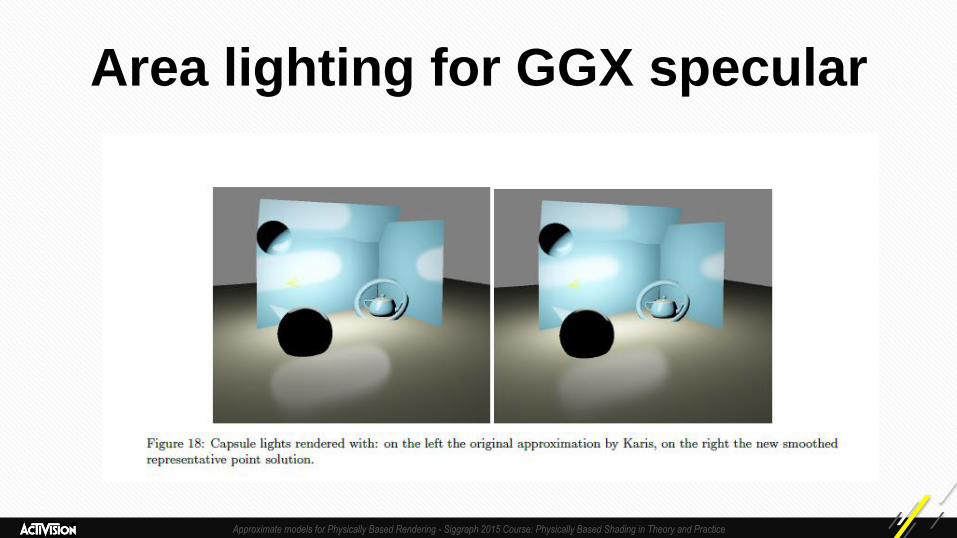
Area lighting for GGX specular
Approximate models for Physically Based Rendering - Siggraph 2015 Course: Physically Based Shading in Theory and Practice
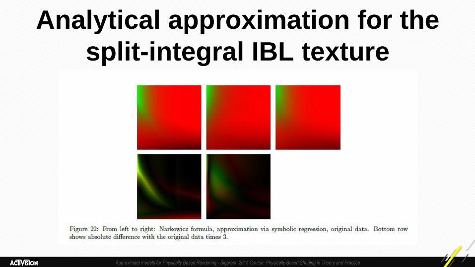
Analytical approximation for the
split-integral IBL texture
Approximate models for Physically Based Rendering - Siggraph 2015 Course: Physically Based Shading in Theory and Practice
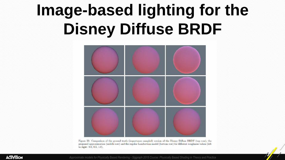
Image-based lighting for the
Disney Diffuse BRDF
Approximate models for Physically Based Rendering - Siggraph 2015 Course: Physically Based Shading in Theory and Practice
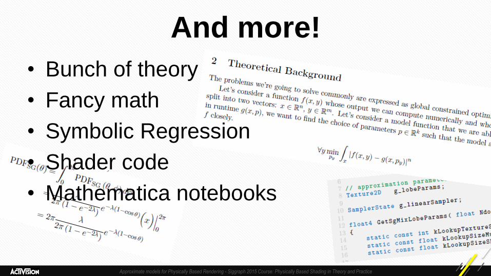
And more!
• Bunch of theory
• Fancy math
• Symbolic Regression
• Shader code
• Mathematica notebooks

Approximate models for Physically Based Rendering - Siggraph 2015 Course: Physically Based Shading in Theory and Practice
Acknowledgments
• Steve Hill, Steve McAuley
• All the smart people we work with, including but
not limited to:
• Peter-Pike Sloan
• Joe Manson
• Mike Stark
• Paul Edelstein
• Jorge Jimenez
• Danny Chan
• Dave Blizard
• Demetrius Leal
• Dimitar Lazarov

Approximate models for Physically Based Rendering - Siggraph 2015 Course: Physically Based Shading in Theory and Practice
Q&A
Contact us (we mean it): [email protected]
[email protected], @kenpex


