
AQUATOX Short Course SETAC Meeting, Portland Oregon
November 7, 2010
Richard A. Park, Eco Modeling, Diamondhead MS [email protected]
Jonathan S. Clough, Warren Pinnacle Consulting, Warren VT [email protected]
Marjorie Coombs Wellman, Office of Water, US EPA, Washington [email protected]

Introduction to Course, Organization
• Schedule and administrative details
• CD organization
– Directory Setup
– For those with laptops, files to look at during the day

Overview: What is AQUATOX?
• Simulation model that links pollutants to aquatic life
• Integrates fate & ecological effects
– nutrient & eutrophication effects
– fate & bioaccumulation of organics
– food web & ecotoxicological effects
• Predicts effects of multiple stressors
– nutrients, organic toxicants
– temperature, suspended sediment, flow
• Can be evaluative (with “canonical” or representative environments) or site-specific
• Peer reviewed by independent panels and in several published model reviews
• Distributed by US EPA, Open Source code

Why AQUATOX?• A truly integrated eutrophication, contaminant
fate and effect model– “is the most complete and versatile model described in the
literature” (Koelmans et al. 2001)
– “Probably… the most advanced environmental model worldwide. ” in review of 17 ecological models (Kianirad et al. 2006)
– CATS-5 (Traas et al. 2001) is similar; models microcosms
– CASM (Bartell et al. 1999) models toxic effects but not fate
• Can simulate many more types of organisms with more realism than most other water quality models– WASP7 models total phytoplankton and benthic algae (Wool
et al. 2004, Ambrose et al. 2006); zooplankton are just a grazing term; no grazing or sloughing of benthic algae
– QUAL2K models phytoplankton and “bottom algae” (Chapra
and Pelletier 2003); no animals
• Comprehensive bioaccumulation model

Acceptance of AQUATOX
• Has gone through 2 EPA-sponsored peer reviews (following quotes from 2008 review):– “model enhancements have made AQUATOX one
of the most exciting tools in aquatic ecosystem management”
– “this is the first model that provides a reasonable interface for scientists to explore ecosystem level effects from multiple stressors over time”
– “the integration of ICE data into AQUATOX makes this model one of the most comprehensive aquatic ecotoxicology programs available”
– it “would make a wonderful textbook for an ecotoxicology class”
• Is gradually appearing in open literature

Potential Applications for AQUATOX
• Many waters are impaired biologically as well as chemically
• Managers need to know:– What is the most important stressor?
– Will proposed actions reverse the impairment?• restoration of desirable aquatic community and/or
designated uses
• improved chemical water quality
– Will there be any unintended consequences?
– How long will recovery take?
– Uncertainty around predictions

Regulatory Endpoints Modeled
• Nutrient and toxicant concentrations
• Biomass– plant, invertebrate, fish
• Chlorophyll a – phytoplankton, periphyton, moss
• Biological metrics
• Total suspended solids, Secchi depth
• Dissolved oxygen– daily minimum and maximum
• Biochemical oxygen demand
• Bioaccumulation factors
• Half-lives of organic toxicants

Potential Applicationsnutrients
• Develop nutrient targets for rivers, lakes and reservoirs subject to nuisance algal blooms
• Evaluate which factor(s) is controlling algae levels– nutrients, suspended sediments, grazing, herbicides, flow
• Evaluate effects of agricultural practices or land use changes– Will target chlorophyll a concentrations be attained after
BMPS are implemented?
– Will land use changes from agriculture to residential use increase or decrease eutrophication effects?
– Linkage to watershed models in BASINS

Potential Applications of AQUATOXtoxic substances
• Ecological risk assessment of chemicals– Will non-target organisms be harmed?
• Will sublethal effects cause game fish to disappear?
– Will there be disruptions to the food web?• Will reduction of zooplankton reduce the food supply for
beneficial fish?
• Or will it lead to nuisance algae blooms?
• Bioaccumulative compounds– Calculate BAFs and tissue concentrations
– Estimate time until fish are safe to eat after remediation

Potential Applicationsaquatic life support
• Evaluate proposed water quality criteria– Support designated use?
• Estimate recovery time of community after reducing pollutants
• Evaluate potential responses to invasive species and mitigation measures– Impacts on native species?– Changes in ecosystem “services”?
• Evaluate possible effects of climate change– Link to climate and/or watershed models

Comparison of Dynamic Risk Assessment Models
State Variables & Processes
AQUATOX CATS CASM Qual2K WASP7EFDC-HEM3D
QEAFdChn BASS QSim
Nutrients X X X X X X X
Sediment Diagenesis X X X X
Detritus X X X X X X X
Dissolved Oxygen X X X X X X
DO Effects on Biota X X
pH X X X
NH4 Toxicity X
Sand/Silt/Clay X X X
SABS Effects X
Hydraulics X X
Heat Budget X X X X
Salinity X X X
Phytoplankton X X X X X X X
Periphyton X X X X X X
Macrophytes X X X X
Zooplankton X X X X
Zoobenthos X X X X
Fish X X X X X
Bacteria X X
Pathogens X X
Organic Toxicant Fate X X X X
Organic Toxicants in:
Sediments X X X X
Stratified Sediments X X X
Phytoplankton X X
Periphyton X X
Macrophytes X X
Zooplankton X X X
Zoobenthos X X X
Fish X X X X
Birds or other animals
X X
Ecotoxicity X X X X
Linked Segments X X X X X X

Comparison of Bioaccumulation Models: Biotic State Variables
Imhoff et al. 2004
Table 3.2. Comparison of Bioaccumulation State Variables
AQ
UA
TO
X R
el e
ase 2
BA
SS
v 2
.1B
iotic L
i gand
1.0
.0E
cofa
te 1
. 0b
1, G
ob
as
EM
CM
1.0
RA
MA
S E
co
syste
mQ
EA
FD
CH
N 1
.0T
RIM
.FaT
E v
3.3
BIOTIC STATE VARIABLES
Plants
Single Generalized Water Column Algal Species 7
Multiple Generalized Water Column Algal Species
Green Algae
Blue-green Algae
Diatoms
Single Generalized Benthic Algal Species 7
Multiple Generalized Benthic Algal Species
Periphyton 7
Macrophytes
Animals
Generalized Compartments for Invertebrates or Fish
Generalized Zooplankton Species 7
Detritivorous Invertebrates 4
Herbivorous Invertebrates 3
Predatory Invertebrates
Single Generalized Fish Species
Multiple Generalized Fish Species
Bottom Fish
Forage Fish 3
Small Game Fish
Large Game Fish 3
Fish Organ Systems 6
Age / Size Structured Fish Populations 5
Marine Birds
Additional Mammals

What AQUATOX does not do
• It does not model metals– Hg was attempted, but unsuccessful
• It does not model bacteria or pathogens– microbial processes are implicit in
decomposition
• It does not model temperature regime and hydrodynamics
– easily linked with hydrodynamic model

AQUATOX Structure
• Time-variable– variable-step 4th-5th order Runge-Kutta
• usually daily reporting time step• can use hourly time-step and reporting
• Spatially simple unless linked to hydrodynamic model– thermal stratification– salinity stratification (based on salt balance)
• Modular and flexible– written in object-oriented Pascal (Delphi)– model only what is necessary (flask to river)– multi-threaded, multiple document interface
• Control vs. perturbed simulations

AQUATOX Simulates Ecological Processes & Effects within a Volume of Water Over Time
Inorganic Sediment
Nutrients (NO3,NH3,PO4)
Organictoxicant
Detritus (suspended,
particulate, dissolved, sedimented )
Oxygen
PlantsPhytoplanktonAttached algaeMacrophytes
Suspended sediment(TSS, Sand/silt/clay)
Ingestion
PhotosynthesisRespiration
Light extinction
AnimalsInvertebrates (spp)
Fish (spp)
Settling, resuspension
Partitioning
En
vir
on
me
nta
l lo
ad
ing
s
Ou
tflo
w

Processes Simulated
• Bioenergetics
– feeding, assimilation
– growth, promotion, emergence
– reproduction
– mortality
– trophic relations
– toxicity (acute & chronic)
• Environmental fate
– nutrient cycling
– oxygen dynamics
– partitioning to water, biota & sediments
– bioaccumulation
– chemical transformations
– biotransformations
• Environmental effects
– direct & indirect

Ecosystem components
detritus
piscivore
forage fish(t. level 3)
phytoplankton
zooplankton (trophic level 2)
zoobenthos
macrophyte
(trophic level 1)
periphyton
detritivore

State Variables in Coralville, Iowa, Study

State Variables in Experimental Tank

AQUATOX Capabilities(Release 3 in red)
• Ponds, lakes, reservoirs, streams, rivers, estuaries
• Riffle, run, and pool habitats for streams
• Completely mixed, thermal stratification, or salinity stratification
• Linked segments, tributary inputs
• Multiple sediment layers with pore waters
• Sediment Diagenesis Model
• Diel oxygen and low oxygen effects, ammonia toxicity
• Interspecies Correlation Estimation (ICE) toxicity database
• Variable stoichiometry, nutrient mass balance, TN & TP
• Dynamic pH
• Biota represented by guilds, key species
• Constant or variable loads
• Latin hypercube uncertainty, nominal range sensitivity analysis
• Wizard & help files, multiple windows, task bar
• Links to HSPF and SWAT in BASINS

Release 3.1 (Currently in beta release)
• 64-bit-compatible software installer
• Updated ICE toxicity regressions
• Improved uncertainty & sensitivity output
• Additional outputs for diagenesis & bioaccumulation
• Improved database export & search capabilities
• More flexible linkage to HSPF watershed model
• In progress:
– Technical Documentation and interface refinements
– Testing bioaccumulation refinements.
– Diagenesis optimization?
Beta available at warrenpinnacle.com AQUATOX page
Demonstration 1
How is AQUATOX used? Overview of user-friendly graphical interface
Installation Considerations
The “APS” and “ALS” file units
Looking at a few Parameters
Libraries of Parameters
Looking at Model Output vs. Observed
Setup Screen
Integrated Help-File and Users Manual

What are the Analytical Capabilities?
• Graphical Analysis
– Comparison of model results to Observed Data
– Graph types and graph libraries
• Control-Perturbed Comparisons
• Process Rates
• Limitations to Photosynthesis
• Sensitivity Analysis
• Uncertainty Analysis

The Many Types of AQUATOX Output (in order of output list)
• Concentrations of State Variables– toxicants in water– nutrients and gasses– organic matter, plants, invertebrates, fish
• Physical Characteristic State Variables– water volume, temperature, wind, light, pH
• Mass of Toxicants within State Variables (normalized to water volume)– T1-T20 in organic matter, plants, invertebrates, and fish
• Additional Model Calculations– Secchi depth, chlorophyll a, velocity, TN, TP, BOD
• Biological metrics– % EPT, Chironomids, Amphipods, % Blue-Greens, Diatoms,
Greens, Gross Primary Production, Turnover, Trophic State Indices

The Many Types of AQUATOX Output (continued)
• Sediment diagenesis state variables
• Toxicant PPB– T1-T20 (PPB) in organic matter, plants, invertebrates, and
fish
• Nitrogen and Phosphorus Mass Tracking Variables
• Bioaccumulation Factors
• Uptake, Depuration, and Bioconcentration Factors
• State Variable Rates
• Limitations to Photosynthesis
• Observed data imported by user
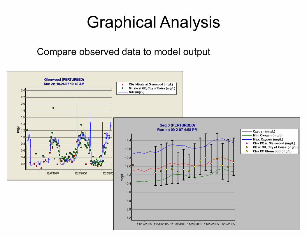
Graphical Analysis
Compare observed data to model output
Obs Nitrate at Glenwood (mg/L)
Nitrate at GB, City of Boise (mg/L)NO3 (mg/L)
Glenwood (PERTURBED)
Run on 10-24-07 10:40 AM
12/5/200112/5/200012/6/1999
mg/L
2.4
2.2
2.0
1.8
1.6
1.4
1.2
1.0
0.8
0.6
0.4
0.2
Oxygen (mg/L)Min. Oxygen (mg/L)
Max. Oxygen (mg/L)Obs DO at Glenwood (mg/L)DO at GB, City of Boise (mg/L)
Obs DO Glenwood (mg/L)
Seg 3 (PERTURBED)Run on 09-2-07 4:58 PM
12/2/200511/29/200511/26/200511/23/200511/20/200511/17/2005
mg/L
14.4
13.6
12.8
12.0
11.2
10.4
9.6
8.8
8.0
7.2

Graphical AnalysisPercent exceedance, duration, scatter plots, log-scale graphs
P e r i L o w -N u t D ( g /m 2 d r y)
P e r i H ig h -N u t (g /m 2 d r y)
P e r i , N a v ic u la ( g /m 2 d r y )
P e r i , N i tz s c h i ( g / m 2 d r y)
C la d o p h o r a ( g /m 2 d r y )
P e r i , G r e e n (g / m 2 d r y)P e r i , B l u e - G r e (g / m 2 d r y)
P h y t H ig h - N u t (m g / L d r y )
P h y t L o w - N u t D (m g / L d r y )
P h y t o , G r e e n ( m g /L d r y )
P h y t , B l u e -G r e ( m g /L d r y )
C r yp t o m o n a s ( m g /L d r y)
G le n w o o d ( P E RT U R B E D )
R u n o n 1 0 - 2 4 -0 7 1 0 : 4 0 A M
1 2 /5 /20 0 112 /5 /2 00 01 2 /6 /19 9 9
g/m
2 d
ry
2 7. 0
2 4. 3
2 1. 6
1 8. 9
1 6. 2
1 3. 5
1 0. 8
8 .1
5 .4
2 .7
0 .0
mg/L d
ry
1. 1
1. 0
0. 9
0. 8
0. 7
0. 6
0. 5
0. 4
0. 3
0. 2
0. 1
0. 0
O b s A m m o n i a a t G le n w o o d ( m g / L )A m m o n i a at G B , C it y o f B o is e ( m g / L )N H 3 & N H 4 + (m g / L )
G l e n w o o d ( P E R T UR B E D )R u n o n 1 0 - 2 4 - 0 7 1 0 : 4 0 A M
1 2 /4 /20 0 51 2 /5 /2 00 31 2/ 5/ 20 011 2/ 6/ 19 9 912 /6 /1 9 97
mg/L
0 .4 0
0 .3 6
0 .3 2
0 .2 8
0 .2 4
0 .2 0
0 .1 6
0 .1 2
0 .0 8
0 .0 4
0 .0 0
O b s B O D a t G le n w o o d ( m g /L )
B O D a t G B , C i ty o f B o is e ( m g / L)
B O D 5 ( m g /L )
G le n w o o d ( P E R T U R BE D)
Ru n o n 1 0 -2 4 - 0 7 10 : 4 0 AM
12 /4 /2 0 051 2/ 5 /2 00 31 2/ 5 /2 00 11 2/ 6 /1 99 9
mg/L
4 .4
4 .0
3 .6
3 .2
2 .8
2 .4
2 .0
1 .6
1 .2
. 8
. 4
P e r i. C h lo r o p h y ll (m g /s q .m )
P e r i C h l a a t G le n w o o d ( m g/ s q .m )
G l e n w o o d ( P E R T U RB E D )
R u n o n 1 0 -2 4 - 0 7 1 0 : 4 0 A M
1 2/ 5/ 2 00 112 /5 /2 0 001 2/ 6/ 1 99 9
mg/sq.m
1 89 .0
1 68 .0
1 47 .0
1 26 .0
1 05 .0
8 4. 0
6 3. 0
4 2. 0
2 1. 0
0 .0
O x yg e n ( m g /L )M in . O xy g e n ( m g /L )M a x. O x y g e n ( m g /L )O b s D O a t G le n w o o d ( m g / L )D O at G B , C it y o f B o is e ( m g / L )
G l e n w o o d ( P E R T U RB E D )R u n o n 1 0 -2 4 - 0 7 1 0 : 4 0 A M
8/ 25 /2 00 12/2 4 /2 00 18 /2 6/2 0 002/ 26 /2 00 08/ 28 /1 99 92 /2 7 /19 9 9
mg/L
1 5. 2
1 4. 4
1 3. 6
1 2. 8
1 2. 0
1 1. 2
1 0. 4
9 .6
8 .8
8 .0
O b s P O 4 a t G le n w o o d ( m g / L )
T o t. S o l. P (m g /L )
T P a t G B , C i ty o f B o is e ( m g /L )
T P (m g /L )
G le n w o o d ( P E R T U R BE D)
Ru n o n 1 0 - 2 4- 0 7 1 0: 4 0 AM
12 /4 / 20 0512 /5 /2 0 0312 /5 / 20 011 2/ 6/ 1 99 91 2/ 6 /1 99 7m
g/L
0 .7
0 .6
0 .6
0 .5
0 .4
0 .4
0 .3
0 .2
0 .1
0 .1
mg/L
1. 1
1. 0
0. 9
0. 8
0. 7
0. 6
0. 5
0. 4
0. 3
0. 2
0. 1
0. 0
Graph Library saved within simulation

Comparing Scenarios: the “Difference” Graph
100%
Control
ControlPerturbed
Result
Result-ResultDifference
Difference graph designed to capture the percent change in results due to perturbation:
Phyt High-Nut
Peri High-Nut
Myriophyllum
Gastropod
ShinerLargemouth Bas
Largemouth Ba2
FARM POND, ESFENVAL (Difference) (Epilimnion Segment)
4/11/19952/10/199512/12/199410/13/19948/14/19946/15/1994
% D
IFFEREN
CE
400.0
350.0
300.0
250.0
200.0
150.0
100.0
50.0
0.0
-50.0
-100.0
The perturbation caused
Myriophyllum to decrease by 81%
on 9/21/1994

Process Rates
• Concentrations of state variables are solved using differential equations– For example, the equation for periphyton concentrations
is:
• Individual terms of these equations may be saved internally, and graphed to understand the basis for various predictions
Peri
Peri
SedPredationMortality
ExcretionnRespiratioesisPhotosynthLoadingdt
dBiomass

Rates Plot Example: Periphyton
Peri High-Nut (g/m2 dry)
Peri High-Nut Load (Percent)Peri High-Nut Photosyn (Percent)
Peri High-Nut Respir (Percent)Peri High-Nut Excret (Percent)Peri High-Nut Other Mort (Percent)
Peri High-Nut Predation (Percent)Peri High-Nut Sloughing (Percent)
Blue Earth R.MN (54) (PERTURBED)Run on 03-25-08 12:29 PM
11/10/20007/13/20003/15/200011/16/19997/19/19993/21/1999
g/m
2 d
ry
13.5
12.0
10.5
9.0
7.5
6.0
4.5
3.0
1.5
.0
Perc
ent
50
45
40
35
30
25
20
15
10
5
Biomass
Sloughing
Predation
Photosynthesis

Limitations to Photosynthesis May also be Graphed
Peri High-Nut Lt_LIM (frac)
Peri High-Nut Nutr_LIM (frac)
Peri High-Nut Temp_LIM (frac)
Blue Earth R.MN (54) (PERTURBED)Run on 03-25-08 12:29 PM
10/11/20007/13/20004/14/20001/15/200010/17/19997/19/19994/20/19991/20/1999
frac
1.0
0.9
0.8
0.7
0.6
0.5
0.4
0.3
0.2
0.1
0.0
Light Limit
Nutrient Limit
Temp. Limit

Integrated Nominal Range Sensitivity Analysis with Graphics
Sensitivity of Peri. Chlorophyll (mg/sq.m) to 20% change in tested parameters3/21/2008 9:56:56 AM
Peri. Chlorophyll (mg/sq.m)
1101009080
21.2% - Peri, Green: Exponential Mort. Coefficient: (max / d) * Linked *
23.5% - Peri, Green: N Half-saturation (mg/L) * Linked *
24.2% - Phyto, Green: N Half -saturation (mg/L) * Linked *
24.8% - Peri, Navicula: N Half -saturation (mg/L) * Linked *
24.8% - Phyt Low -Nut D: N Half-saturation (mg/L) * Linked *
29.2% - Phyt High-Nut : Max Photosynthetic Rate (1/d) * Linked *
33% - Peri Low -Nut D: Optimal Temperature (deg. C) * Linked *
45.1% - Phyt High-Nut : Optimal Temperature (deg. C) * Linked *
61.3% - Peri, Green: Max Photosynthetic Rate (1/d) * Linked *
68.5% - Phyto, Green: Max Photosynthetic Rate (1/d) * Linked *
91.7% - Phyto, Green: Optimal Temperature (deg. C) * Linked *
101% - Peri, Green: Optimal Temperature (deg. C) * Linked *

Integrated Latin Hypercube Uncertainty Analysis with Graphics
Mean
MinimumMaximumMean - StDev
Mean + StDevDeterministic
Smallmouth Bas (g/m2)3/21/2008 10:15:57 AM
11/10/20007/13/20003/15/200011/16/19997/19/19993/21/1999
0.5
0.48
0.46
0.44
0.42
0.4
0.38
0.36
0.34
0.32
0.3
0.28
0.26
0.24
0.22
can represent all “point estimate” parameters as distributions

Physical Characteristics of a Site
Modeled Waterbody
Deeply Buried Sediment
Sediment Active Layer (Well Mixed)
Water Inflow Water Discharge
Evaporation
Water Balance and Sediment Structure

Thermal Stratification in a Lake

Stratification is a function of temperature differences
Increased mixing is also a function of discharge
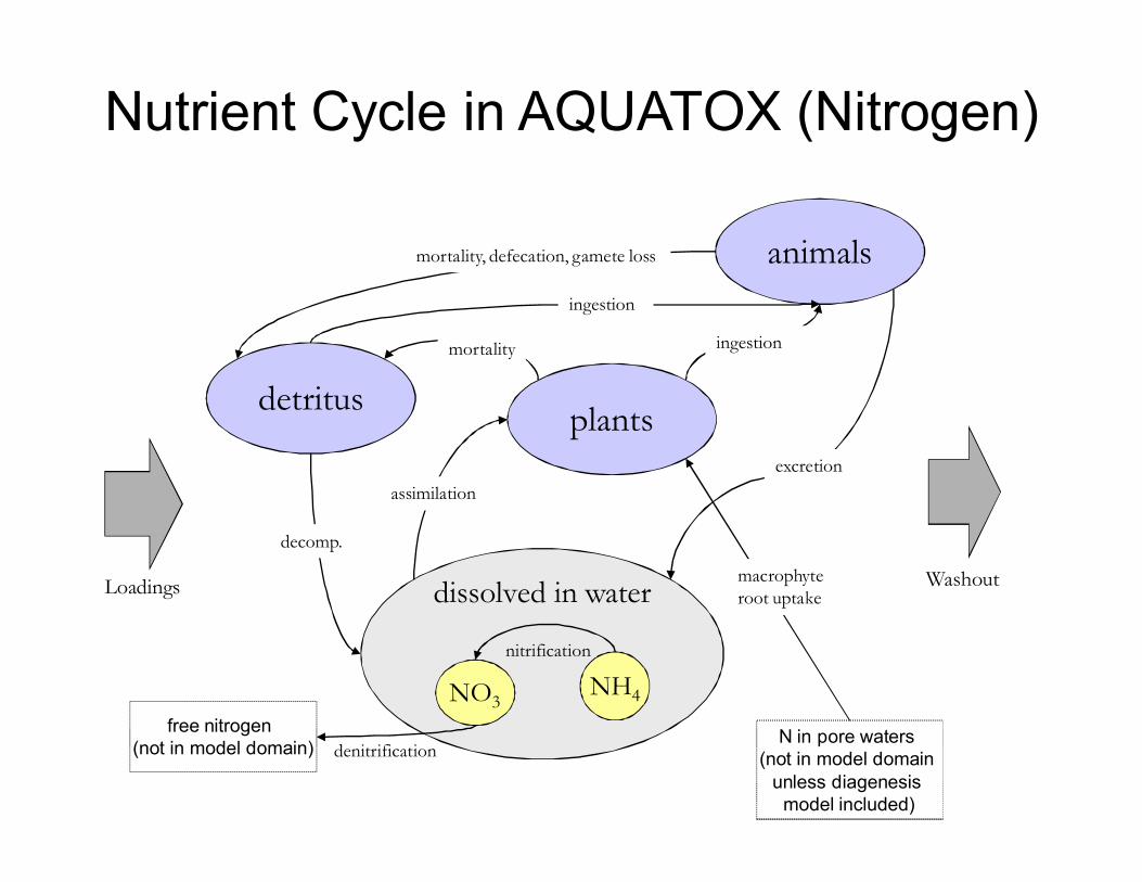
detritus
dissolved in water
Nutrient Cycle in AQUATOX (Nitrogen)
NH4NO3
nitrification
denitrification
plants
animals
assimilation
mortality
mortality, defecation, gamete loss
Loadings Washout
excretion
N in pore waters (not in model domain
unless diagenesis model included)
macrophyte root uptake
free nitrogen (not in model domain)
decomp.
ingestion
ingestion

Nutrient Cycle in AQUATOX (Phosphorus)
detritus
phosphate
dissolved in water
plants
animals
assimilation
mortality
mortality, defecation, gameteloss
Loadings Washout
excretion,
respiration
P in pore waters
(outside model domain)
macrophyte
root uptake
decomp.
ingestion
ingestion
excretion, respiration
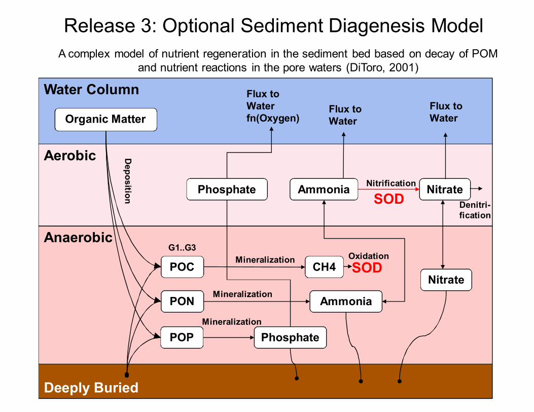
Deeply Buried
Anaerobic
Aerobic
Phosphate Ammonia Nitrate
POC
POP
PON Ammonia
Phosphate
Mineralization
Mineralization
Mineralization
Nitrification
Nitrate
Water ColumnFlux to Water
Flux to Water fn(Oxygen)Organic Matter
Dep
ositio
n
Release 3: Optional Sediment Diagenesis Model
A complex model of nutrient regeneration in the sediment bed based on decay of POM and nutrient reactions in the pore waters (DiToro, 2001)
Flux to Water
G1..G3
SOD
SODOxidation
CH4
Denitri-fication

Key Points: Diagenesis Model
• Two sediment layers: thin aerobic and thicker anaerobic
• When oxygen is present, the diffusion of phosphorus from sediment pore waters is limited – Strong P sorption to oxidated ferrous iron in the aerobic layer
(iron oxyhydroxide precipitate)
– Under conditions of anoxia, phosphorus flux from sediments dramatically increases.
• Sediment oxygen demand (SOD) is a function of specific chemical reactions following the decomposition of organic matter
– methane or sulfide production
– nitrification of ammonia

Nutrient Effects on Simulations
• Direct effects on algal growth rates– Maximum growth rates often limited by
nutrients
– Degree of limitation may be tracked and plotted
• Indirect repercussions throughout the foodweb due to bottom-up effects
• Light climate changes due to algal blooms
• Algal composition will be affected
• Decomposition of organic matter affects oxygen concentrations

Applications in Nutrient Analysis
• Lake Onondaga, NY
• Rum, Blue Earth, and Crow Wing Rivers, MN
• Cahaba River, AL
• Lower Boise River, ID
• Lake Tenkiller, OK
• Florida streams
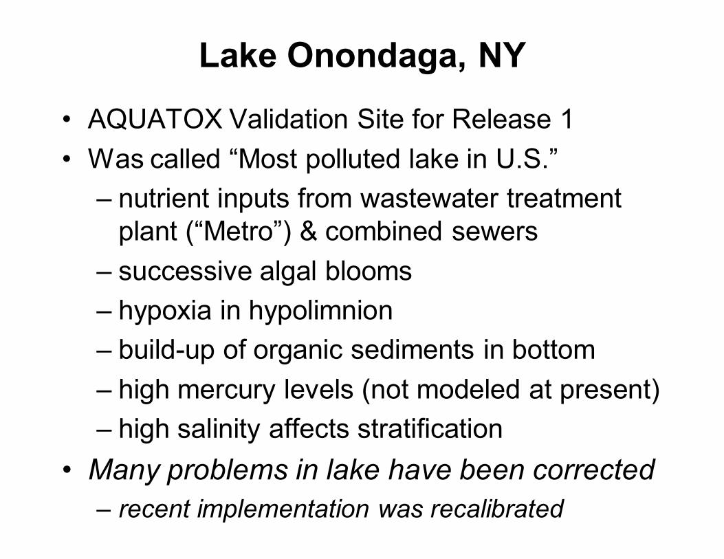
Lake Onondaga, NY
• AQUATOX Validation Site for Release 1
• Was called “Most polluted lake in U.S.”
– nutrient inputs from wastewater treatment plant (“Metro”) & combined sewers
– successive algal blooms
– hypoxia in hypolimnion
– build-up of organic sediments in bottom
– high mercury levels (not modeled at present)
– high salinity affects stratification
• Many problems in lake have been corrected
– recent implementation was recalibrated

Lake Onondaga NY, heavily polluted

Phyto. Chlorophyll (ug/L)
Obs Chl a (ug/L)
ONONDAGA LAKE, NY (PERTURBED) Run on 11-3-07 3:53 PM(Epilimnion Segment)
1/2/19919/4/19905/7/19901/7/19909/9/19895/12/19891/12/1989
ug/L
95
85
76
66
57
47
38
28
19
9
Lake Onondaga was very productive with succession of algal groups
Cyclote lla nan (mg/L dry)
Greens (mg/L dry)Phyt, Blue-Gre (m g/L dry)
Cryptomonad (mg/L dry)
ONONDAGA LAKE, NY (PERTURBED) Run on 11-3-07 3:53 PM
(Epilimnion Segment)
1/2/19919/4/19905/7/19901/7/19909/9/19895/12/19891/12/1989
mg/L
dry
4.5
4.0
3.5
3.0
2.5
2.0
1.5
1.0
.5
.0

Hypolimnion goes anoxic with high SOD
Oxygen (m g/L)
Obs H DO (mg/L)
ONONDAGA LAKE, NY (PERTURBED) Run on 11-3-07 3:53 PM(Hypolimnion Segment)
1/2/19919/4/19905/7/19901/7/19909/9/19895/12/19891/12/1989
mg/L
14.0
12.6
11.2
9.8
8.4
7.0
5.6
4.2
2.8
1.4
.0
SOD (gO2/m2 d)
Oxygen (mg/L)
ONONDAGA LAKE, NY (PERTURBED) Run on 11-3-07 3:53 PM(Hypolimnion Segment)
1/2/19919/4/19905/7/19901/7/19909/9/19895/12/19891/12/1989
gO
2/m
2 d
0.8
0.7
0.6
0.5
0.4
0.4
0.3
0.2
0.1
0.0
mg/L
14.0
12.6
11.2
9.8
8.4
7.0
5.6
4.2
2.8
1.4
.0

Hypolimnion phosphorus is better modeled bysediment diagenesis submodel
NH3 & NH4+ (m g/L)
NO3 (mg/L)Tot. Sol. P (m g/L)
ONONDAGA LAKE, NY (PERTURBED) Run on 11-3-07 3:53 PM
(Hypolimnion Segment)
1/2/19919/4/19905/7/19901/7/19909/9/19895/12/19891/12/1989
mg/L
4.0
3.6
3.2
2.8
2.4
2.0
1.6
1.2
.8
.4
.0
NH3 & NH4+ (mg/L)
NO3 (mg/L)
Tot. Sol. P (mg/L)
ONONDAGA LAKE, NY (PERTURBED) Run on 11-2-07 1:52 PM(Hypolimnion Segment)
1/2/19919/4/19905/7/19901/7/19909/9/19895/12/19891/12/1989
mg/L
4.0
3.6
3.2
2.8
2.4
2.0
1.6
1.2
.8
.4
.0
“Classic” AQUATOX model (P is blue)
Sediment diagenesis model (note >P release)

Oxygen (mg/L)
Hypolimnion O2 (mg/L)
ONONDAGA LAKE, NY (CONTROL) Run on 10-9-09 11:49 AM
(Hypolimnion Segment)
1/2/19919/4/19905/7/19901/7/19909/9/19895/12/19891/12/1989
mg/L
14.0
12.6
11.2
9.8
8.4
7.0
5.6
4.2
2.8
1.4
.0
Oxygen (mg/L)
Hypolimnion O2 (mg/L)
ONONDAGA LAKE, NY (PERTURBED) Run on 10-9-09 11:38 AM(Hypolimnion Segment)
1/2/19919/4/19905/7/19901/7/19909/9/19895/12/19891/12/1989
mg/L
14.0
12.6
11.2
9.8
8.4
7.0
5.6
4.2
2.8
1.4
.0
What if Metro WWTP effluent were diverted?
With Metro diversion, anoxia does not occur
With Metro effluent

Validation of AQUATOX with Lake Onondaga Data—visual test

Validation with chlorophyll a in Lake Onondaga, NY
Kolmogorov-Smirnov p statistic = 0.319 (not significantly different)

Release 3 Addition: Calcium Carbonate Precipitation
• Predicted as a function of pH and algal type
– When pH exceeds 7.5, precipitation is predicted
– Precipitation rate is dependent on photosynthesis rate (gross primary production) in some, but not all, algae
• CaCO3 sorbs phosphate from the water column
CaCO3 Precip. (m g/L d)
GPP (gO2/m2 d)
ONONDAGA LAKE, NY (PERTURBED) Run on 11-15-09 8:53 AM(Epilimnion Segment)
9/8/19903/10/19909/9/19893/11/1989
mg/L
d
9.0
8.1
7.2
6.3
5.4
4.5
3.6
2.7
1.8
.9
.0
gO2/m
2 d
19.0
17.1
15.2
13.3
11.4
9.5
7.6
5.7
3.8
1.9
0.0

Modeling Phytoplankton
• Phytoplankton may be greens, blue-greens, diatoms or “other algae”
• Subject to sedimentation, washout, and turbulent diffusion
• In stream simulations, assumptions about flow and upstream production are important

Modeling Periphyton
• Periphyton are not simulated by most water quality models
• Periphyton are difficult to model
– include live material and detritus
– stimulated by nutrients
– snails & other animals graze it heavily
– riparian vegetation reduces light to stream
– build-up of mat causes stress & sloughing, even at relatively low velocity
• Many water body impairments due to periphyton
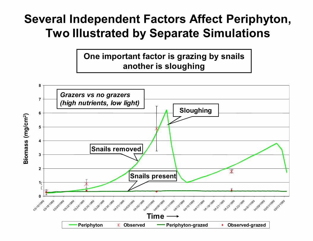
Several Independent Factors Affect Periphyton, Two Illustrated by Separate Simulations
0
1
2
3
4
5
6
7
8
Periphyton Observed Periphyton-grazed Observed-grazed
Grazers vs no grazers(high nutrients, low light)
One important factor is grazing by snailsanother is sloughing
Snails removed
Snails present
Time
Sloughing

Modeling Macrophytes
• Macrophytes may be specified as benthic, rooted-floating, or free-floating
• Macrophytes can have significant effect on light climate and other algae communities
• Root uptake of nutrients is assumed and mass balance tracked
• May act as refuge from predation for animals
• Leaves can provide significant surface area for periphyton growth
• Moss are a special category

Calibration of Plants
• algae are differentiated on basis of:
– nutrient half-saturation values
– light saturation values
– maximum photosynthesis
• Minnesota stream project has developed new parameter sets that span nutrient, light, and Pmax
– See AQUATOX Technical Note 1: A Calibrated Parameter Set for Simulation of Algae in Shallow Rivers
• phytoplankton sedimentation rates differ between running and standing water
• critical force for periphyton scour and TOpt may need to calibrated for other sites

Minnesota Streams Project
Low nutrientlow turbidity
Moderate nutrientmoderate turbidity
High nutrienthigh turbidity

Calibration Strategy for Minnesota Rivers
• Must be able to simulate changing conditions!
• Add plants and animals representative of both low- (Crow Wing) and high-nutrient (Blue Earth) rivers
• Iteratively calibrate key parameters for each site and cross-check to make sure they still hold for other siteo Used linked version for simultaneous calibration
across sites
• When goodness-of-fit is acceptable for both sites, apply to an intermediate site (Rum River) and reiterate calibration across all three sites
• Parameter set was validated with Cahaba River AL data

State variables in MN rivers simulations

Chlorophyll a Trends in MN Rivers
1: Phyto. Chlorophyll (ug/L)
2: Phyto. Chlorophyll (ug/L)3: Phyto. Chlorophyll (ug/L)
Obs. BE chl a (ug/L)Obs CWR chl a (ug/L)
Obs RR chl a (ug/L)
Linked MN Rivers (CONTROL)Run on 07-18-07 9:32 PM
11/10/20007/13/20003/15/200011/16/19997/19/19993/21/1999
ug/L
360
324
288
252
216
180
144
108
72
36
1: Peri. Chlorophyll (mg/sq.m)
2: Peri. Chlorophyll (mg/sq.m)
3: Peri. Chlorophyll (mg/sq.m)
Obs. BE peri chl a (mg/sq.m)Obs. CWR peri chl a (mg/sq.m)
Obs. RR peri chl a (mg/sq.m)
Linked MN Rivers (CONTROL)Run on 07-18-07 9:32 PM
11/10/20007/13/20003/15/200011/16/19997/19/19993/21/1999
mg/s
q.m
48
43
38
34
29
24
19
14
10
5
Phytoplankton follow nutrient trend
Periphyton reach maximum in Rum River with moderate
nutrients and turbidity

0
50
100
150
200
250
300
350
400
01/99 05/99 08/99 12/99 04/00 08/00 12/00
chl_
a (u
g/L
)
Observed (symbols) and calibrated AQUATOX simulations (lines) of chlorophyll a in Blue Earth River at mile 54
0
10
20
30
40
50
60
70
01/99 05/99 08/99 12/99 04/00 08/00 12/00
chl_
a (u
g/L
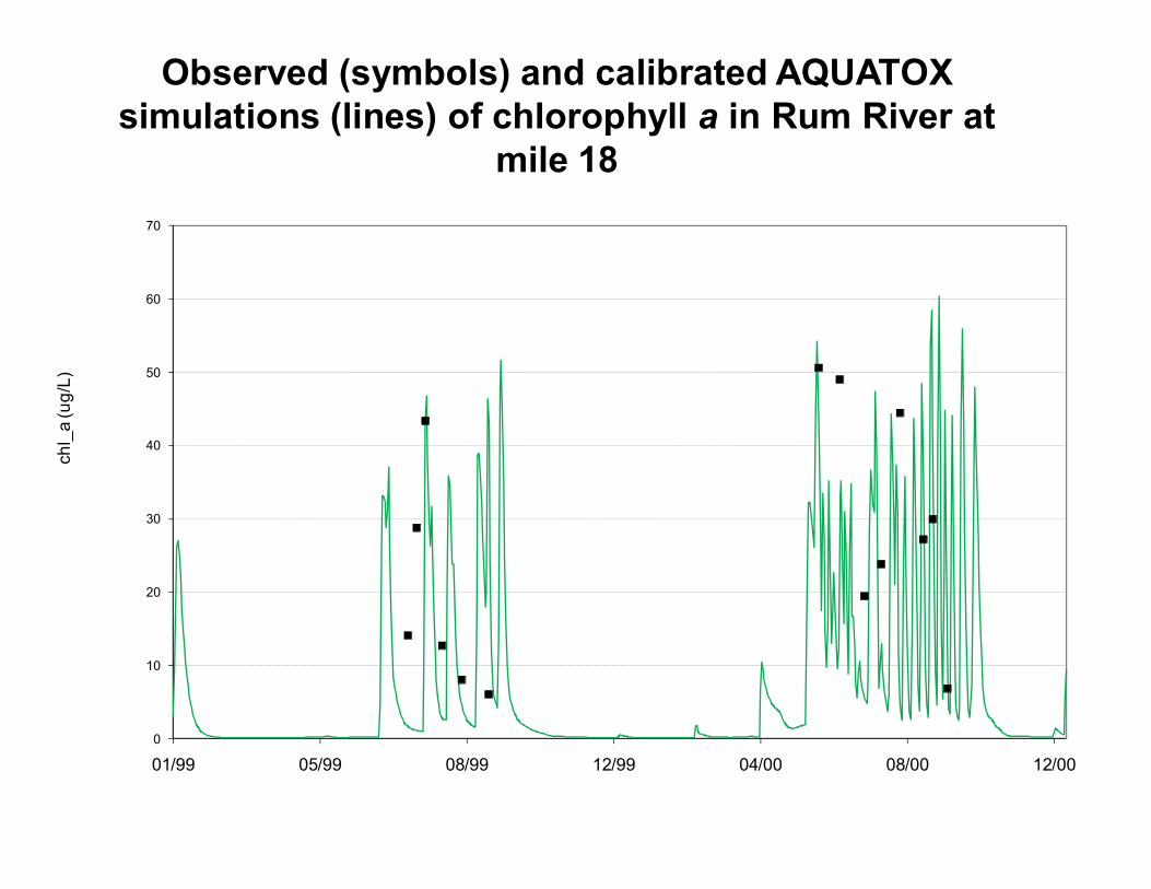
)Observed (symbols) and calibrated AQUATOX
simulations (lines) of chlorophyll a in Rum River at mile 18
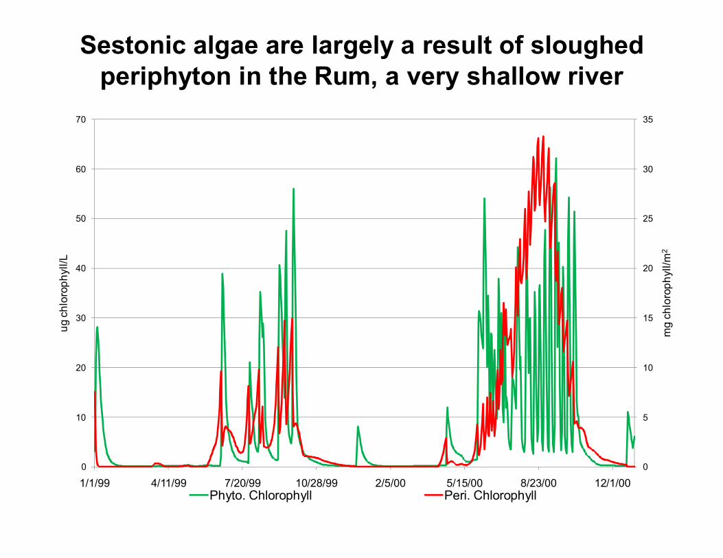
Sestonic algae are largely a result of sloughed periphyton in the Rum, a very shallow river
0
5
10
15
20
25
30
35
0
10
20
30
40
50
60
70
1/1/99 4/11/99 7/20/99 10/28/99 2/5/00 5/15/00 8/23/00 12/1/00
mg
ch
loro
ph
yll/m
2
ug
ch
loro
ph
yll/L
Phyto. Chlorophyll Peri. Chlorophyll

0
5
10
15
20
25
30
01/99 05/99 08/99 12/99 04/00 08/00 12/00
chl_
a (
ug/L
)
Observed (symbols) and calibrated AQUATOX simulations (lines) of chlorophyll a in Crow Wing at mile 72

Summer mean percent phytoplankton composed of cyanobacteria-- BE-54 simulations with fractional
multipliers on TP, TN, and TSS
observed values in larger rivers
observed values in smaller rivers
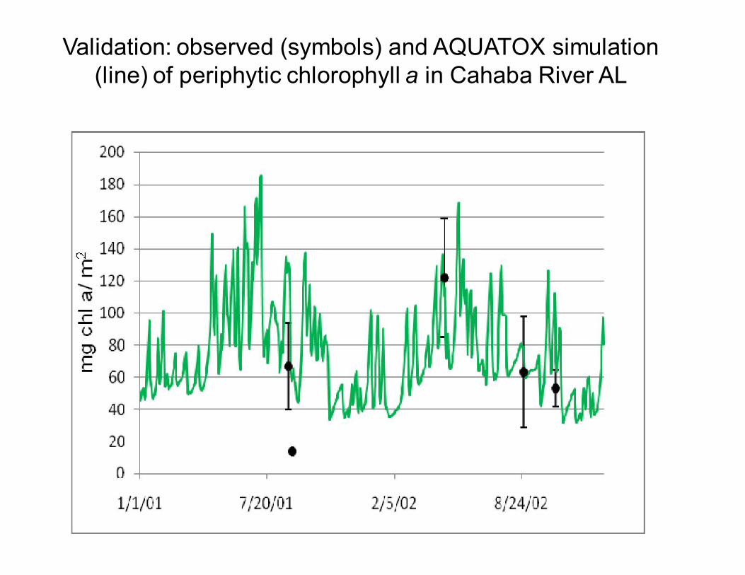
Validation: observed (symbols) and AQUATOX simulation (line) of periphytic chlorophyll a in Cahaba River AL

AQUATOX -- BASINS Linkage
AQUATOXProvides time series loading data and GIS information to
AQUATOX
Creates AQUATOX simulations using physical characteristics of BASINS
watershed
Integrates point/nonpoint source analysis with effects on receiving water and biota

Linkages Between Models
BASINS GIS Layer
WinHSPF
Linkage within BASINS Linkage to AQUATOX(**BASINS 3.1 only)
SWAT**
AQUATOX
GenScn

Use of AQUATOX in Water Quality Management Decisions
• 2008 peer review suggests AQUATOX is suited to support existing approaches used to develop water quality standards and criteria
– One tool among many that should be used in a weight- of-evidence approach
• AQUATOX enables the evaluation of multiple stressor scenarios– What is the most important stressor driving algal
response?
• Go beyond chlorophyll a to evaluate quality, not just quantity, of algal responses (e.g., reduction of blue-green algal blooms)

Minnesota Nutrient Sites
Low nutrientlow turbidity
Moderate nutrientmoderate turbidity
High nutrienthigh turbidity
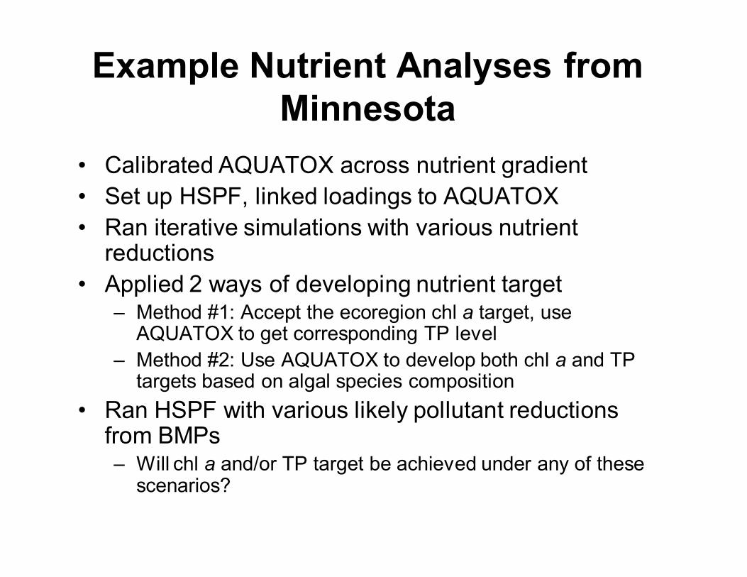
Example Nutrient Analyses from Minnesota
• Calibrated AQUATOX across nutrient gradient
• Set up HSPF, linked loadings to AQUATOX
• Ran iterative simulations with various nutrient reductions
• Applied 2 ways of developing nutrient target– Method #1: Accept the ecoregion chl a target, use
AQUATOX to get corresponding TP level
– Method #2: Use AQUATOX to develop both chl a and TP targets based on algal species composition
• Ran HSPF with various likely pollutant reductions from BMPs– Will chl a and/or TP target be achieved under any of these
scenarios?

Plants
25% reduction TP
0.000
0.200
0.400
0.600
0.800
1.000
1.200
1/1
/199
9
3/1
/199
9
5/1
/199
9
7/1
/199
9
9/1
/199
9
11
/1/1
99
9
1/1
/200
0
3/1
/200
0
5/1
/200
0
7/1
/200
0
9/1
/200
0
11
/1/2
00
0
Plants
25% reduction TSS
0
0.2
0.4
0.6
0.8
1
1.2
1/1
/1999
3/1
/1999
5/1
/1999
7/1
/1999
9/1
/1999
11/1
/1999
1/1
/2000
3/1
/2000
5/1
/2000
7/1
/2000
9/1
/2000
11/1
/2000
Differences in TSS and TP loadings have significant
effects on algal community; BOD appears to have some
effect, though of much shorter duration
Plants
25% reduction Detritus
0
0.2
0.4
0.6
0.8
1
1.2
1/1
/199
9
3/1
/199
9
5/1
/199
9
7/1
/199
9
9/1
/199
9
11/1
/199
9
1/1
/200
0
3/1
/200
0
5/1
/200
0
7/1
/200
0
9/1
/200
0
11/1
/200
0
Step 1: Stressor ID using Biotic IndexAlgal community response dependent upon stressor

Step 2: Run AQUATOX with multiple load reduction scenarios.
Compare Mean TP and Chl a
TP/TSS multiplier Mean TP (ug/L) Mean chl_a (ug/L)
1.0 268 18.3
0.8 214 11.0
0.6 161 9.5
0.4 107 8.2
0.2 54 8.0
0.0 0* 0.2
Ecoregional criterion
118.13 7.85

Step 3a: Water Quality Target Development Method #1
• Focus on TP and chl a only
• according to model: 80% TP reduction required to meet 7.85 ug/L chl a
• according to 304(a) recommendation: 56% TP reduction required to meet same chl a level
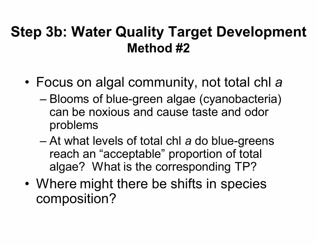
Step 3b: Water Quality Target Development Method #2
• Focus on algal community, not total chl a– Blooms of blue-green algae (cyanobacteria)
can be noxious and cause taste and odor problems
– At what levels of total chl a do blue-greens reach an “acceptable” proportion of total algae? What is the corresponding TP?
• Where might there be shifts in species composition?

Algal Composition Changes Seasonally and from year to year
Phytoplankton biomass
baseline
0
10
20
30
40
50
60
70
1/1
/1999
2/1
/1999
3/1
/1999
4/1
/1999
5/1
/1999
6/1
/1999
7/1
/1999
8/1
/1999
9/1
/1999
10/1
/1999
11/1
/1999
12/1
/1999
1/1
/2000
2/1
/2000
3/1
/2000
4/1
/2000
5/1
/2000
6/1
/2000
7/1
/2000
8/1
/2000
9/1
/2000
10/1
/2000
11/1
/2000
12/1
/2000
Bio
mass (
mg
/L)
0
100
200
300
400
500
600
700
Ch
loro
ph
yll
a (
ug
.L)
Phyt High-Nut (mg/L) Phyt Low-Nut D (mg/L) Phyto, Navicul (mg/L) Phyto, Green (mg/L)
Phyt, Blue-Gre (mg/L) Cryptomonas (mg/L) Chloroph (ug/L)
Blue-greens Chl. a
0.0
4.0
8.0
12.0
16.0
20.0
0.000 0.050 0.100 0.150 0.200 0.250 0.300
mean TP (mg/L)m
ean
ch
loro
ph
yll
_a (
ug
/L)
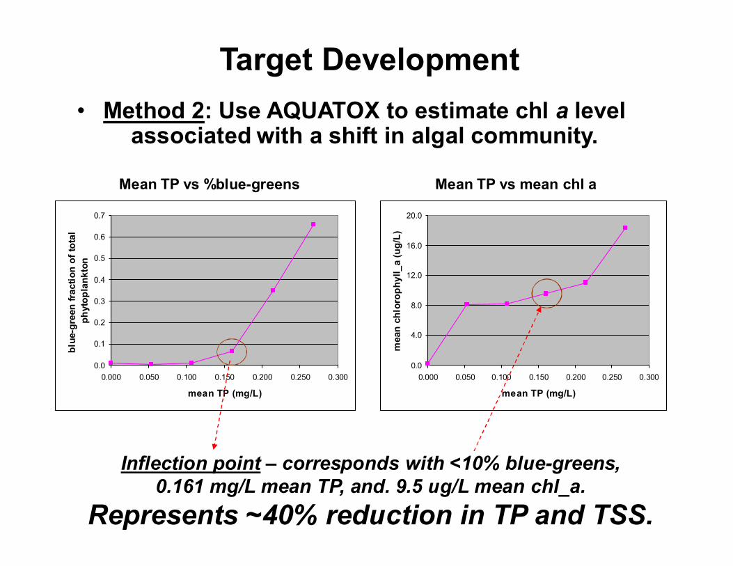
Target Development
• Method 2: Use AQUATOX to estimate chl a level associated with a shift in algal community.
0.0
0.1
0.2
0.3
0.4
0.5
0.6
0.7
0.000 0.050 0.100 0.150 0.200 0.250 0.300
mean TP (mg/L)
blu
e-g
reen
fra
cti
on
of
tota
l
ph
yto
pla
nk
ton
Inflection point – corresponds with <10% blue-greens, 0.161 mg/L mean TP, and. 9.5 ug/L mean chl_a.
Represents ~40% reduction in TP and TSS.
Mean TP vs %blue-greens Mean TP vs mean chl a
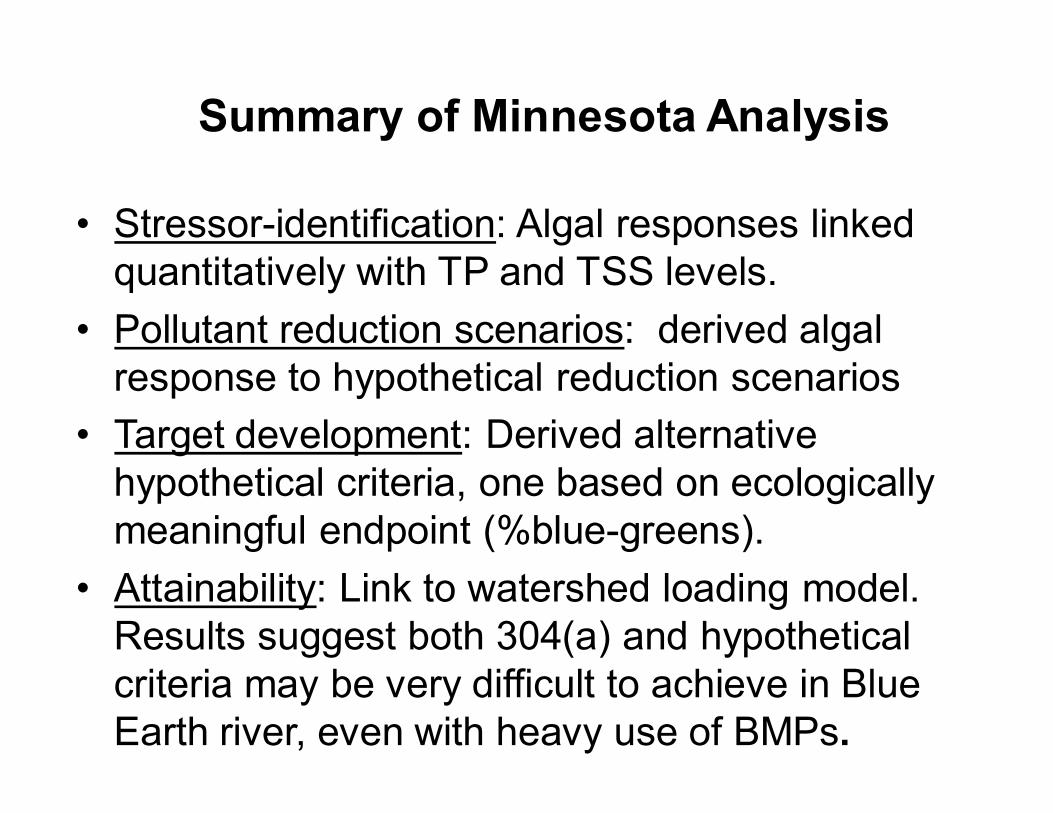
• Stressor-identification: Algal responses linked quantitatively with TP and TSS levels.
• Pollutant reduction scenarios: derived algal response to hypothetical reduction scenarios
• Target development: Derived alternative hypothetical criteria, one based on ecologically meaningful endpoint (%blue-greens).
• Attainability: Link to watershed loading model. Results suggest both 304(a) and hypothetical criteria may be very difficult to achieve in Blue Earth river, even with heavy use of BMPs.
Summary of Minnesota Analysis
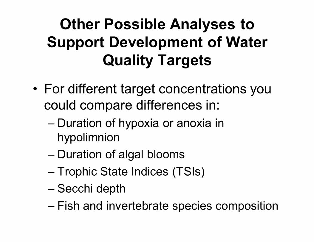
Other Possible Analyses to Support Development of Water
Quality Targets
• For different target concentrations you could compare differences in:
– Duration of hypoxia or anoxia in hypolimnion
– Duration of algal blooms
– Trophic State Indices (TSIs)
– Secchi depth
– Fish and invertebrate species composition
Modeling Animals with AQUATOX
• Overview
• Parameters
• Zooplankton
• Zoobenthos
• Fish
• Trophic Interaction Matrices

Animal Modeling Overview
• Animal biomasses calculated dynamically
– Gains due to consumption and boundary-condition loadings
– Losses due to defecation, respiration, excretion, mortality, predation, boundary condition losses
• Careful specification of feeding preferences required
• Bioenergetic modeling for fish

Animal Parameters

Zooplankton consumption is often tied to phytoplankton productivity
Daphnia Consumption (Percent)
Daphnia Defecation (Percent)
Daphnia Respiration (Percent)
Daphnia Excretion (Percent)
Daphnia TurbDiff (Percent)
Daphnia Predation (Percent)
Daphnia Low O2 Mort (Percent)
Daphnia NH3 Mort (Percent)
Daphnia NH4+ Mort (Percent)
Daphnia Other Mort (Percent)
Daphnia Mortality (Percent)
Daphnia (mg/L dry)
ONONDAGA LAKE, NY (CONTROL) Run on 09-24-08 11:13 AM(Epilimnion Segment)
9/8/19903/10/19909/9/19893/11/1989
Perc
ent
60
54
47
40
33
27
20
13
7
mg/L d
ry
2.7
2.4
2.1
1.8
1.5
1.2
0.9
0.6
0.3
0.0

Benthic invertebrates are also tied to phytoplankton productivity through detritus
Tubifex tubife (g/m2 dry)
Tubifex tubife Consumption (Percent)
Tubifex tubife Defecation (Percent)
Tubifex tubife Respiration (Percent)
Tubifex tubife Excretion (Percent)
Tubifex tubife Predation (Percent)
Tubifex tubife Mortality (Percent)
ONONDAGA LAKE, NY (CONTROL) Run on 09-24-08 11:13 AM(Epilimnion Segment)
9/8/19903/10/19909/9/19893/11/1989
g/m
2 d
ry
0.040
0.038
0.036
0.034
0.032
0.030
0.028
0.026
0.024
0.022
0.020
0.018
Perce
nt
83
75
66
58
50
42
33
25
17
8

Tubifex in hypolimnion are tolerant of anoxia but stop feeding and slowly decline
Tubifex tubife (g/m2 dry)
Tubifex tubife Consumption (Percent)
Tubifex tubife Defecation (Percent)Tubifex tubife Respiration (Percent)
Tubifex tubife Excretion (Percent)
Tubifex tubife Predation (Percent)
Tubifex tubife Mortality (Percent)
ONONDAGA LAKE, NY (CONTROL) Run on 09-24-08 11:13 AM(Hypolimnion Segment)
9/8/19903/10/19909/9/19893/11/1989
g/m
2 d
ry
0.022
0.020
0.018
0.016
0.014
0.012
0.010
0.008
0.006
0.004
Perce
nt
45
41
36
32
27
23
18
14
9
5

Fish exhibit seasonal patternsbased on food availability and temperature
Shad Consumption (Percent)
Shad Defecation (Percent)
Shad Respiration (Percent)Shad Excretion (Percent)
Shad Predation (Percent)
Shad Mortality (Percent)
Shad GameteLoss (Percent)
Shad (g/m2 dry)
ONONDAGA LAKE, NY (CONTROL) Run on 10-8-08 8:13 AM(Epilimnion Segment)
9/8/19903/10/19909/9/19893/11/1989
Perc
ent
15.0
13.5
12.0
10.5
9.0
7.5
6.0
4.5
3.0
1.5
.0
g/m
2 d
ry
14.3
13.0
11.7
10.4
9.1
7.8
6.5
5.2
3.9
2.6

Foodweb Model specified as Trophic MatrixInteractions are normalized to 100%

Lower Boise River, Idaho with WWTPs and agricultural drains
1: Low-nutrient
3: Higher nutrient
13: Highest nutrients,turbidity
10: Higher nutrients
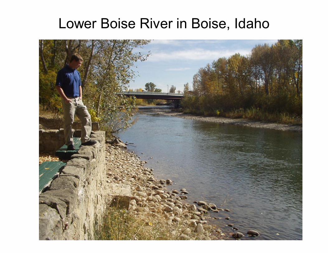
Lower Boise River in Boise, Idaho
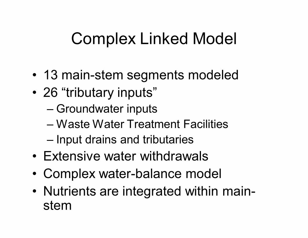
Complex Linked Model
• 13 main-stem segments modeled
• 26 “tributary inputs”– Groundwater inputs
– Waste Water Treatment Facilities
– Input drains and tributaries
• Extensive water withdrawals
• Complex water-balance model
• Nutrients are integrated within main-stem

LBR Downstream Periphyton Trend
S1: Peri. Chlorophyll (mg/sq.m)S2: Peri. Chlorophyll (mg/sq.m)
S3: Peri. Chlorophyll (mg/sq.m)
S4: Peri. Chlorophyll (mg/sq.m)
S5: Peri. Chlorophyll (mg/sq.m)
S6: Peri. Chlorophyll (mg/sq.m)
S7: Peri. Chlorophyll (mg/sq.m)
S8: Peri. Chlorophyll (mg/sq.m)S9: Peri. Chlorophyll (mg/sq.m)
S10: Peri. Chlorophyll (mg/sq.m)
S11: Peri. Chlorophyll (mg/sq.m)
S12: Peri. Chlorophyll (mg/sq.m)
S13: Peri. Chlorophyll (mg/sq.m)
Linked LBR (PERTURBED)Run on 10-24-07 10:37 PM
12/5/200112/5/200012/6/1999
mg/s
q.m
270.0
243.0
216.0
189.0
162.0
135.0
108.0
81.0
54.0
27.0
0.0
Reach 10
Reach 13
Reach 1
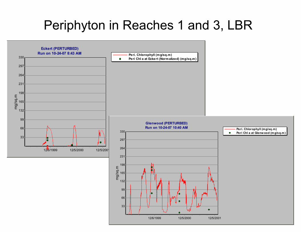
Peri. Chlorophyll (mg/sq.m)Peri Chl a at Eckert (Normalized) (mg/sq.m)
Eckert (PERTURBED)
Run on 10-24-07 8:43 AM
12/5/200112/5/200012/6/1999
mg/s
q.m
330
297
264
231
198
165
132
99
66
33
Periphyton in Reaches 1 and 3, LBR
Peri. Chlorophyll (mg/sq.m)
Peri Chl a at Glenw ood (m g/sq.m )
Glenwood (PERTURBED)Run on 10-24-07 10:40 AM
12/5/200112/5/200012/6/1999
mg/s
q.m
330
297
264
231
198
165
132
99
66
33

Periphyton in Reaches 10 and 13, LBR
Peri. Chlorophyll (mg/sq.m)
Peri Chl a at Caldw ell (mg/sq.m )
Caldwell (PERTURBED)Run on 10-24-07 7:48 PM
12/5/200112/5/200012/6/1999
mg/s
q.m
330
297
264
231
198
165
132
99
66
33
Peri Chl a at Parma (Norm/ (mg/sq.m)
Peri. Chlorophyll (mg/sq.m)
Parma (PERTURBED)Run on 10-24-07 10:37 PM
12/5/200112/5/200012/6/1999
mg/s
q.m
330
297
264
231
198
165
132
99
66
33

LBR Downstream Phytoplankton Trend
S1: Phyto. Chlorophyll (ug/L)
S2: Phyto. Chlorophyll (ug/L)
S3: Phyto. Chlorophyll (ug/L)
S4: Phyto. Chlorophyll (ug/L)
S5: Phyto. Chlorophyll (ug/L)
S6: Phyto. Chlorophyll (ug/L)
S7: Phyto. Chlorophyll (ug/L)
S8: Phyto. Chlorophyll (ug/L)
S9: Phyto. Chlorophyll (ug/L)
S10: Phyto. Chlorophyll (ug/L)
S11: Phyto. Chlorophyll (ug/L)
S12: Phyto. Chlorophyll (ug/L)
S13: Phyto. Chlorophyll (ug/L)
Linked LBR (PERTURBED)Run on 10-24-07 10:37 PM
8/25/20012/24/20018/26/20002/26/20008/28/19992/27/1999
ug/L
43
39
34
30
26
22
17
13
9
4
Reach 13
Reach 2

Sestonic algae at Parma (Reach 13), bothupstream loadings and periphyton sloughing
Obs Chla at Parm a (ug/L)
Phyto. Chlorophyll (ug/L)
Parma (PERTURBED)Run on 10-24-07 10:37 PM
8/25/20012/24/20018/26/20002/26/20008/28/19992/27/1999
ug/L
42
38
34
29
25
21
17
13
8
4

Phytoplankton Sensitivity, Parma LBRcould choose parameters for better fit
Red lines indicate a “negative” parameter
change

Demonstration 2: Linked Segment Version
• Developed as part of a Superfund project; now part of Release 3
• Allows the capability to model multiple linked segments--converting AQUATOX into a two dimensional model
• State variables move from one linked segment to the next through water flow,
diffusion, bed-load, and migration.

Segmented Version can Represent Dynamically Linked Multiple Segments

1
23
4
5
6
6b
7 8 9
10
12
13 14
11
x
y
Feedback Seg.
Cascade Seg.
Feedback Link
Cascade Link
Cascade & Feedback Linkages
Cascade Linkages:
One-way linkages with no backwards flow or diffusion across segment boundaries
Feedback Linkages:
Two-way linkages that allow for backwards flow and diffusion

Linked Segment Model Data Requirements
• Water flows between segments
• Initial conditions for all state variables for each segment modeled
– All segments must have the same state variables
• Inflows, point-sources and non-point-source loadings for each segment
• Tributary or groundwater inputs and/or any withdrawals
Interface Demonstration to follow

Tenkiller Lake, OK

Tenkiller Lake Background
• Reservoir in eastern Oklahoma formed by the damming of the Illinois River (1947-1952)
• Identified on Oklahoma's 1998 303(d) list as impaired (nutrients)
• High-priority target for TMDL development
• 1996 Clean Lakes Study: nutrient concentrations and water clarity are indicative of eutrophic conditions

Tenkiller Lake Application
• Linked Model application includes nine segments– Riverine segment
– Vertically stratified transitional segment
– Three vertically stratified lacustrine segments
• Model linkage to HSPF (watershed) and EFDC (in-lake hydrology) models
• Model can predict chlorophyll a levels based on nutrient loadings (BMPs)
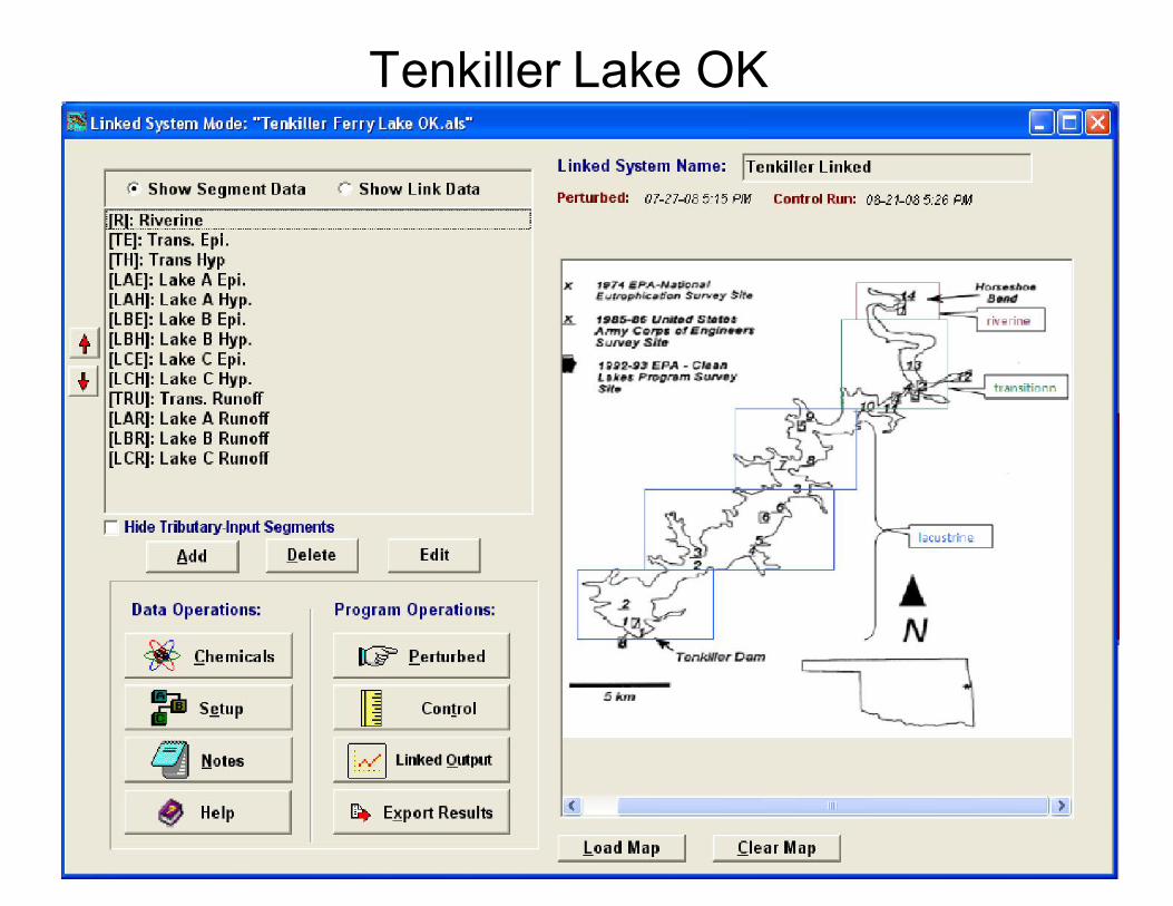
Tenkiller Lake OK

Storm-water plume, algae-rich riverine segment
duckweed (Lemna sp.) forms surface scum at the interface
upstream

R: TP (mg/L)
TE: TP (mg/L)
TH: TP (mg/L)
LAE: TP (mg/L)
LAH: TP (mg/L)
LBE: TP (mg/L)
LBH: TP (mg/L)
LCE: TP (mg/L)
LCH: TP (mg/L)
Tenkiller Linked (CONTROL)Run on 07-8-09 10:17 AM
12/17/19938/19/19934/21/199312/22/19928/24/19924/26/199212/28/1991
mg/L
0.4
0.4
0.4
0.3
0.3
0.2
0.2
0.2
0.1
0.1
0.0
Total phosphorus in water column decreases toward dam; loss to sediments is simulated
Lacustrine C epi
Lacustrine B epi
Transition epi
Riverine

Simulated hypoxia in hypolimnion of Lacustrine A

Simulated & observed algal composition in epilimnetic Transition

Simulated & observed chlorophyll a in Lacustrine A
Phyto. Chlorophyll (ug/L)
Obs chl a 5 (ug/L)
Lake A Epi. (CONTROL)Run on 07-8-09 10:17 AM
12/17/19938/19/19934/21/199312/22/19928/24/19924/26/199212/28/1991
ug/L
57
51
46
40
34
28
23
17
11
6
Diatom bloom
Blue-green bloom

Predicted chlorophyll a in Lacustrine A with 30% and 90% load reduction of TP compared
to baseline (red)
Phyto. Chlorophyll (ug/L)
LAE Chl 90 reduction (ug/L)
LAE Chl 30 reduction (ug/L)
Lake A Epi. (CONTROL)Run on 07-8-09 10:17 AM
12/17/19938/19/19934/21/199312/22/19928/24/19924/26/199212/28/1991
ug/L
57
51
46
40
34
28
23
17
11
6
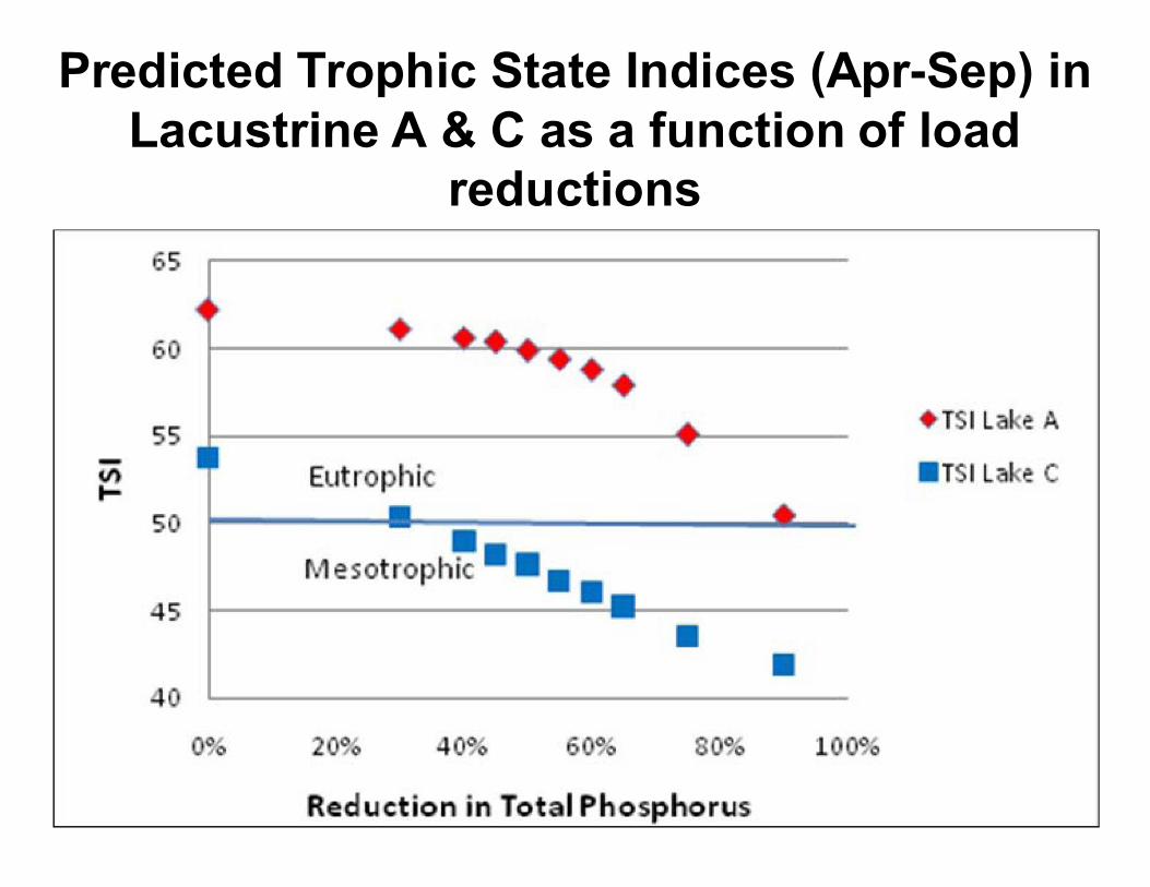
Predicted Trophic State Indices (Apr-Sep) in Lacustrine A & C as a function of load
reductions

Model is being applied to numerous FL streams, including the Suwannee River
Peri. Biomass (g/m2 dry)
Obs peri (thick) (g/m2 dry)
Obs peri AFDW (g/m2 dry)
Upper Suwannee River FL (PERTURBED)Run on 11-5-09 9:00 AM
12/4/200712/4/200512/5/2003
g/m
2 d
ry
11.0
9.9
8.8
7.7
6.6
5.5
4.4
3.3
2.2
1.1
.0
DRAFT

Can diagnose algal response
Eunotia Photosyn (Percent)
Eunotia Respir (Percent)
Eunotia Excret (Percent)
Eunotia Other Mort (Percent)
Eunotia Predation (Percent)
Eunotia Sloughing (Percent)
Upper Suwannee River FL (PERTURBED)Run on 11-5-09 9:00 AM
12/4/200712/4/200512/5/2003
Perc
ent
50
45
40
35
30
25
20
15
10
5
Eunotia Temp_LIM (frac)
Eunotia Lt_LIM (frac)
Eunotia N_LIM (frac)Eunotia PO4_LIM (frac)
Eunotia CO2_LIM (frac)
Upper Suwannee River FL (PERTURBED)Run on 11-5-09 9:00 AM
12/3/200812/4/200712/4/200612/4/200512/4/200412/5/2003
frac
1.0
0.9
0.8
0.7
0.6
0.5
0.4
0.3
0.2
0.1
Sloughing is important
Grazing by mayflies
Nitrogen is limiting
Light is more limiting
DRAFT

Peri. Biomass (g/m2 dry)
Obs peri AFDW (g/m2 dry)
Little Withlacoochee River FL (PERTURBED)Run on 10-11-09 10:58 PM
12/3/200812/4/200712/4/200612/4/2005
g/m
2 d
ry
8.1
7.2
6.3
5.4
4.5
3.6
2.7
1.8
.9
.0
The Little Withlacoochee River has mean TP of 0.044 mg/L
Dri
ed
up
P lim
itati
on
DRAFT

AQUATOX– Chemical Fate Overview
• Can model up to twenty chemicals simultaneously
• Fate processes:– microbial degradation
– photolysis
– ionization
– hydrolysis
– volatilization
– sorption
• Biotransformation—can model daughter products
• Bioaccumulation
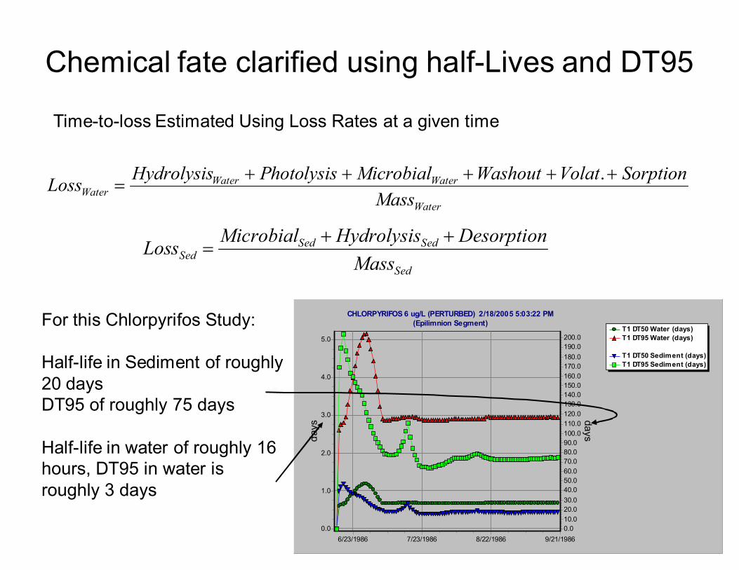
Chemical fate clarified using half-Lives and DT95
T1 DT50 Water (days)
T1 DT95 Water (days)
T1 DT50 Sediment (days)
T1 DT95 Sediment (days)
CHLORPYRIFOS 6 ug/L (PERTURBED) 2/18/2005 5:03:22 PM(Epilimnion Segment)
9/21/19868/22/19867/23/19866/23/1986
da
ys
5.0
4.0
3.0
2.0
1.0
0.0
da
ys
200.0
190.0
180.0
170.0
160.0
150.0
140.0
130.0
120.0
110.0
100.0
90.0
80.0
70.0
60.0
50.0
40.0
30.0
20.0
10.0
0.0
Time-to-loss Estimated Using Loss Rates at a given time
Water
WaterWaterWater
Mass
SorptionVolatWashoutMicrobialPhotolysisHydrolysisLoss
.
Sed
SedSedSed
Mass
DesorptionHydrolysisMicrobialLoss
For this Chlorpyrifos Study:
Half-life in Sediment of roughly 20 daysDT95 of roughly 75 days
Half-life in water of roughly 16 hours, DT95 in water is roughly 3 days
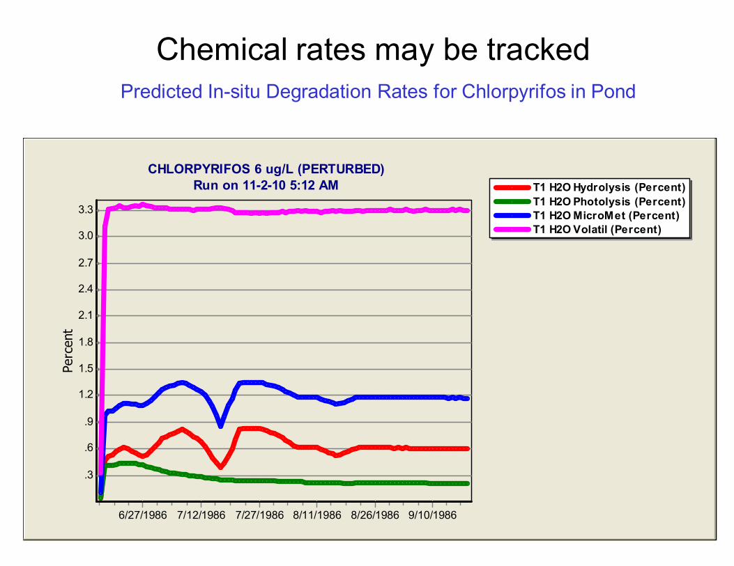
Predicted In-situ Degradation Rates for Chlorpyrifos in Pond
Chemical rates may be tracked
T1 H2O Hydrolysis (Percent)
T1 H2O Photolysis (Percent)
T1 H2O MicroMet (Percent)
T1 H2O Volatil (Percent)
CHLORPYRIFOS 6 ug/L (PERTURBED)Run on 11-2-10 5:12 AM
9/10/19868/26/19868/11/19867/27/19867/12/19866/27/1986
Perc
ent
3.3
3.0
2.7
2.4
2.1
1.8
1.5
1.2
.9
.6
.3
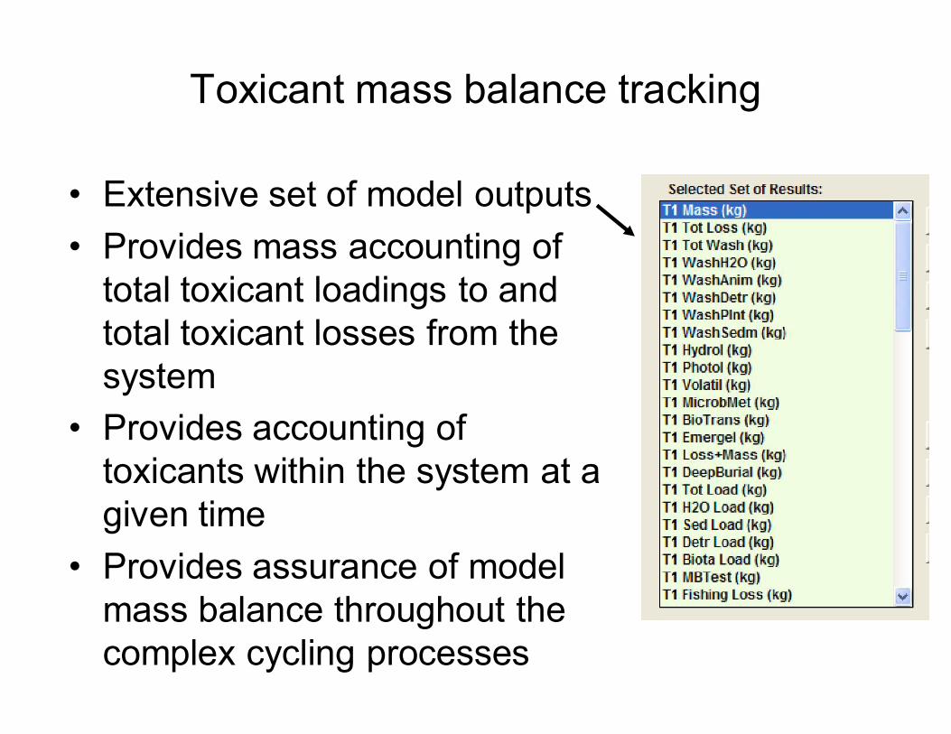
Toxicant mass balance tracking
• Extensive set of model outputs
• Provides mass accounting of total toxicant loadings to and total toxicant losses from the system
• Provides accounting of toxicants within the system at a given time
• Provides assurance of model mass balance throughout the complex cycling processes
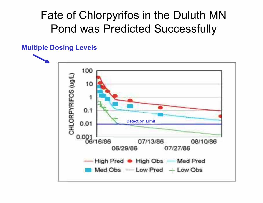
Fate of Chlorpyrifos in the Duluth MN Pond was Predicted Successfully
Multiple Dosing Levels
Detection Limit
HCB in tank
• Reproduces experimental results (Gobas) in which macrophytes are enclosed in an aquarium tank
• A single dose of hexachlorobenzene is applied at the beginning of the simulation
• Simplest type of AQUATOX model setup
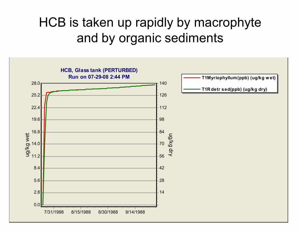
HCB is taken up rapidly by macrophyte and by organic sediments
T1Myriophyllum(ppb) (ug/kg w et)
T1R detr sed(ppb) (ug/kg dry)
HCB, Glass tank (PERTURBED)Run on 07-29-08 2:44 PM
9/14/19888/30/19888/15/19887/31/1988
ug/k
g w
et
28.0
25.2
22.4
19.6
16.8
14.0
11.2
8.4
5.6
2.8
0.0
ug/k
g d
ry
140
126
112
98
84
70
56
42
28
14

T1 H2O Hydrolysis (Percent)
T1 H2O Photolysis (Percent)
T1 H2O MicroMet (Percent)T1 H2O Depuration (Percent)
T1 H2O Volatil (Percent)
T1 H2O DetrSorpt (Percent)
T1 H2O Decom p (Percent)T1 H2O PlantSorp (Percent)
T1 H2O (ug/L)
HCB, Glass tank (PERTURBED)Run on 07-29-08 2:44 PM
9/14/19888/30/19888/15/19887/31/1988
Perc
ent
50
42
34
25
17
8
-8
-17
-25
ug/L
5.4
4.8
4.2
3.6
3.0
2.4
1.8
1.2
.6
HCB loss rates can be plotted, showing that sorption to detritus is negligible (due to mass)
Plant sorption
Volatilization
Depuration
Detrital sorption

Chemical Bioaccumulation Overview
• Kinetic model of uptake and depuration
– Uptake through gill
– Uptake through diet • Consumption rate
• Assimilation efficiency
– Loss through depuration, biotransformation, growth dilution (implicit)
• Alternative (simple) BCF model available

Toxicant in water:• ionization• volatilization• hydrolysis• photolysis• microbial degradation
Losses of toxicant:• predation• mortality• depuration•biotransformation• spawning• promotion• emergence
Uptake through gill:• respiration rate• assimilation efficiency
Uptake from diet• consumption rates• assimilation efficiency • growth rates• toxicity• lipid content
Bioaccumulation in AQUATOX
Toxicant in food sources
• Organic sediments• Algae
• nutrient cycling• loss of predation
Partitioning

Depuration Rate Constants for Invertebrates and Fish

Alternative Chemical Uptake Model
The user may enter two of the three factors defining uptake (BCF,K1, K2) and the third factor is calculated:
(1/d)
d)(L/kg(L/kg)
2
1
K
KBCF
Given these parameters, AQUATOX calculates uptake and depuration in plants and animals as kinetic processes.
Dietary uptake of chemicals by animals is not affected by this alternative parameterization.

Chlorpyrifos in Pond
• Pond enclosure dosed with chlorpyrifos at EPA Duluth lab
• A single dose of chlorpyrifos is applied at the beginning of the simulation
• Additional biotic compartments
– diatoms, greens, invertebrates,
– sunfish, shiner
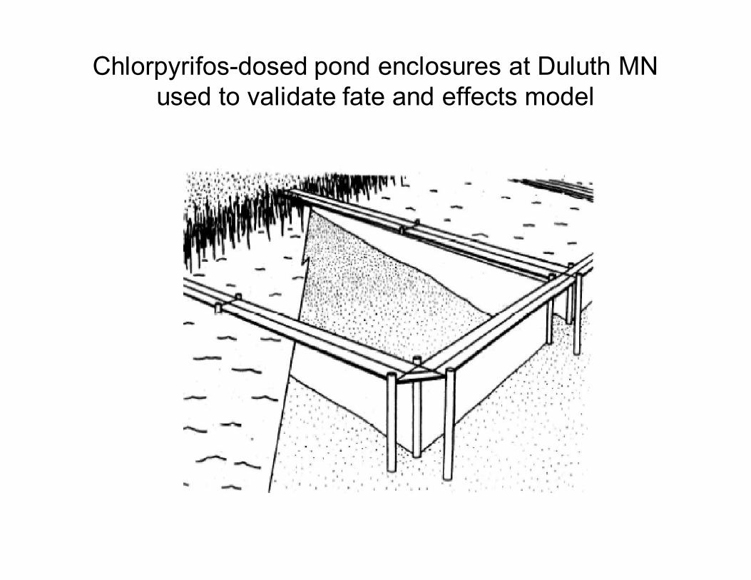
Chlorpyrifos-dosed pond enclosures at Duluth MNused to validate fate and effects model

T1Chironomid(ppb) (ug/kg wet)
T1Daphnia(ppb) (ug/kg wet)
T1Shiner(ppb) (ug/kg wet)
T1Diatoms(ppb) (ug/kg w et)
T1Stigeoclonium,(ppb) (ug/kg wet)
T1Blue-greens(ppb) (ug/kg w et)
T1Chara(ppb) (ug/kg wet)
T1 H2O (ug/L)
CHLORPYRIFOS 6 ug/L (PERTURBED)Run on 11-7-08 12:13 PM
8/26/19867/27/19866/27/1986
ug/k
g w
et
24300.0
21600.0
18900.0
16200.0
13500.0
10800.0
8100.0
5400.0
2700.0
0.0
ug/L
6.3
5.6
4.9
4.2
3.5
2.8
2.1
1.4
.7
.0
Model can trace how the toxicant is partitioned in the biota
Dissolved chlorpyrifos
Chlorpyrifos in shiners
Chlorpyrifos in Daphnia
Chlorpyrifos in phytoplankton

Lake Ontario Bioaccumulation
Observed and predicted lipid-normalized and freely dissolved BAFs for PCBs in Lake Ontario ecosystem components.
4
5
6
7
8
9
10
11
4 5 6 7 8 9
Lo
g B
AF
Log KOW
Phytoplankton
Observed
Predicted
4
5
6
7
8
9
10
11
4 5 6 7 8 9
Lo
g B
AF
Log KOW
Mysids
Observed
Predicted

Lake Ontario Bioaccumulation
Observed and predicted lipid-normalized and freely dissolved BAFs for PCBs in Lake Ontario ecosystem components.
4
5
6
7
8
9
10
11
4 5 6 7 8 9
Lo
g B
AF
Log KOW
Smelt
Observed
Predicted
4
5
6
7
8
9
10
11
4 5 6 7 8 9
Lo
g B
AF
Log KOW
Lake Trout
Observed
Predicted

Lake Ontario BAF model comparison
0.00
1.00
2.00
3.00
4.00
5.00
Pre
d/O
bs
AQUATOX
AQUATOX
GOBAS
THOMANNPerfect correlation

Perfluorinated Surfactants (PFAs)
• Originally developed as part of estuarine model
– Sorption modeled using empirical approach
– Animal Uptake/Depuration a function of chain length and PFA type (sulfonate/ carboxylate)
– Biotransformation can be modeled
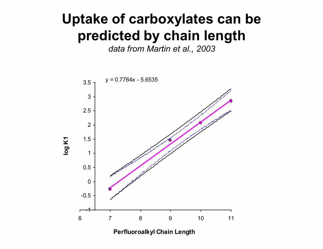
Uptake of carboxylates can be predicted by chain length
data from Martin et al., 2003
y = 0.7764x - 5.6535
-1
-0.5
0
0.5
1
1.5
2
2.5
3
3.5
6 7 8 9 10 11
Perfluoroalkyl Chain Length
log
K1

Depuration rate is also a function of chain length
data from Martin et al., 2003
0
0.02
0.04
0.06
0.08
0.1
0.12
0.14
5 7 9 11 13
Perfluoroalkyl Chain Length
K2
Obs Caboxylate
Pred Carboxylate
Obs Sulfonate
Pred Sulfonate

Estuarine version applied to Galveston Bay, Texas, to evaluate toxicants
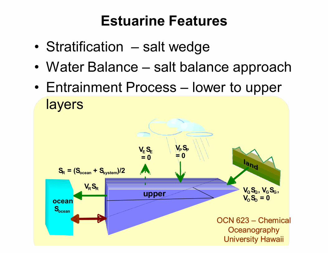
VPSP
= 0VESE
= 0
VQSQ, VGSG, VOSO = 0ocean
Socean
upper
SR = (Socean + Ssystem)/2
VRSR
Estuarine Features
• Stratification – salt wedge
• Water Balance – salt balance approach
• Entrainment Process – lower to upper layers
OCN 623 OCN 623 –– Chemical Chemical OceanographyOceanography
University Hawaii University Hawaii
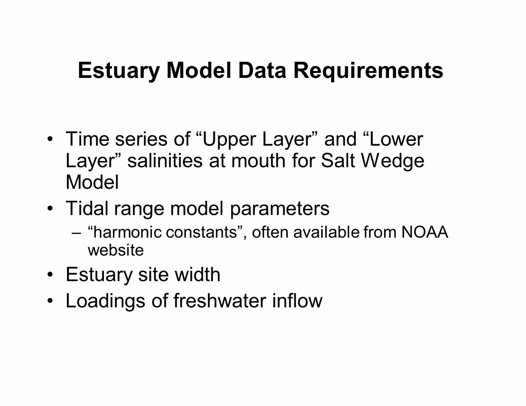
Estuary Model Data Requirements
• Time series of “Upper Layer” and “Lower Layer” salinities at mouth for Salt Wedge Model
• Tidal range model parameters– “harmonic constants”, often available from NOAA
website
• Estuary site width
• Loadings of freshwater inflow

Galveston Bay, Texas, compartments
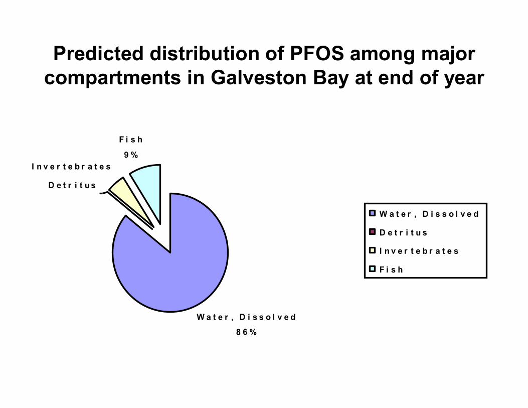
W a t e r , D i s s o l v e d
8 6 %
F i s h
9 %
D e t r i t u s
I n v e r t e b r a t e s
W a t e r , D i s s o l v e d
D e t r i t u s
I n v e r t e b r a t e s
F i s h
Predicted distribution of PFOS among major compartments in Galveston Bay at end of year

Validation: New Bedford Harbor MA, observed & predicted PCB values are comparable
Park et. al, 2008, Figure 7, data from Connolly, 1991Park et. al, 2008, Figure 7, data from Connolly, 1991

Modeling Toxicity of Chemicals
• Lethal and sublethal effects are represented
• Chronic and acute toxicity are both represented
• Effects based on total internal concentrations
• Uses the critical body residue approach (McCarty 1986, McCarty and Mackay 1993)
• Can also model external toxicity– Useful if uptake and depuration are very fast (as
with herbicides)
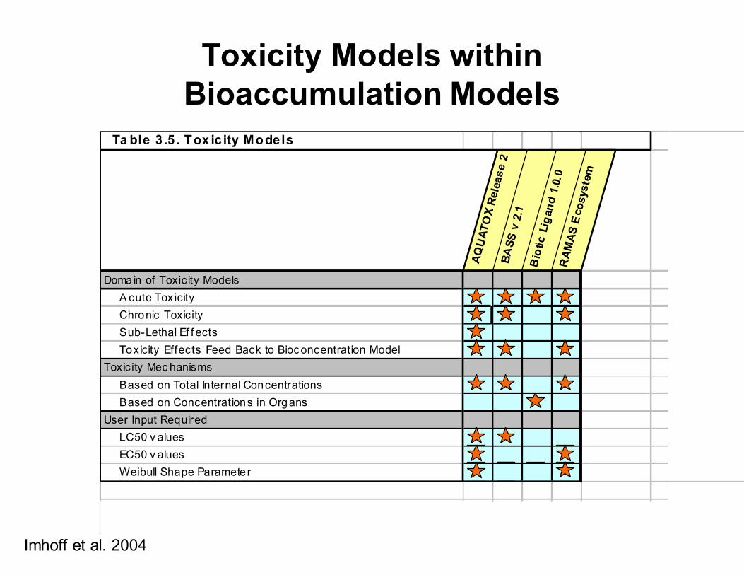
Toxicity Models within Bioaccumulation Models
Ta ble 3 .5 . Tox ic ity Models
AQ
UA
TO
X R
ele
as
e 2
BA
SS
v 2
.1
Bio
tic
Lig
an
d 1
.0.0
RA
MA
S E
co
syste
m
Domain of Toxicity Models
A cute Tox icity
Chronic Toxicity
Sub-Lethal Ef f ects
Toxicity Effects Feed Back to Bioconcentration Model
Toxicity Mec hanisms
Based on Total Internal Concentrations
Based on Concentrations in Organs
User Input Required
LC50 v alues
EC50 v alues
Weibull Shape Parameter
Imhoff et al. 2004

Steps Taken to Estimate Toxicity
• Enter LC50 and EC50 values– LC50 estimators are available for species
• Compute internal LC50
• Compute infinite LC50 (time-independent)
• Compute t-varying internal lethal concentration
• Compute cumulative mortality
• Compute biomass lost per day by disaggregating cumulative mortality
• Sublethal toxicity is related to lethal toxicity through an application factor
• Option has been added to use external concentration.

Disaggregation of Cumulative Mortality
0
0.1
0.2
0.3
0.4
0.5
0.6
0.7
0.8
0.9
1
0 2 4 6 8 10 12 14
days
Cu
mu
lati
ve
Mo
rta
lity
Resistant Fraction Killed
Nonresistant Fraction Killed
dt
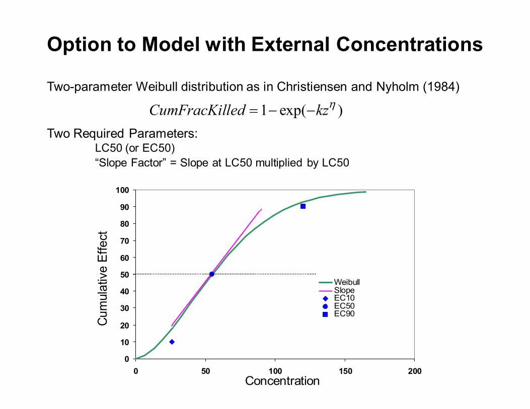
Option to Model with External Concentrations
Two-parameter Weibull distribution as in Christiensen and Nyholm (1984)
)exp(1 kzledCumFracKil
Two Required Parameters: LC50 (or EC50)
“Slope Factor” = Slope at LC50 multiplied by LC50
0
10
20
30
40
50
60
70
80
90
100
0 50 100 150 200
WeibullSlopeEC10EC50EC90
Cum
ula
tive E
ffect
Concentration
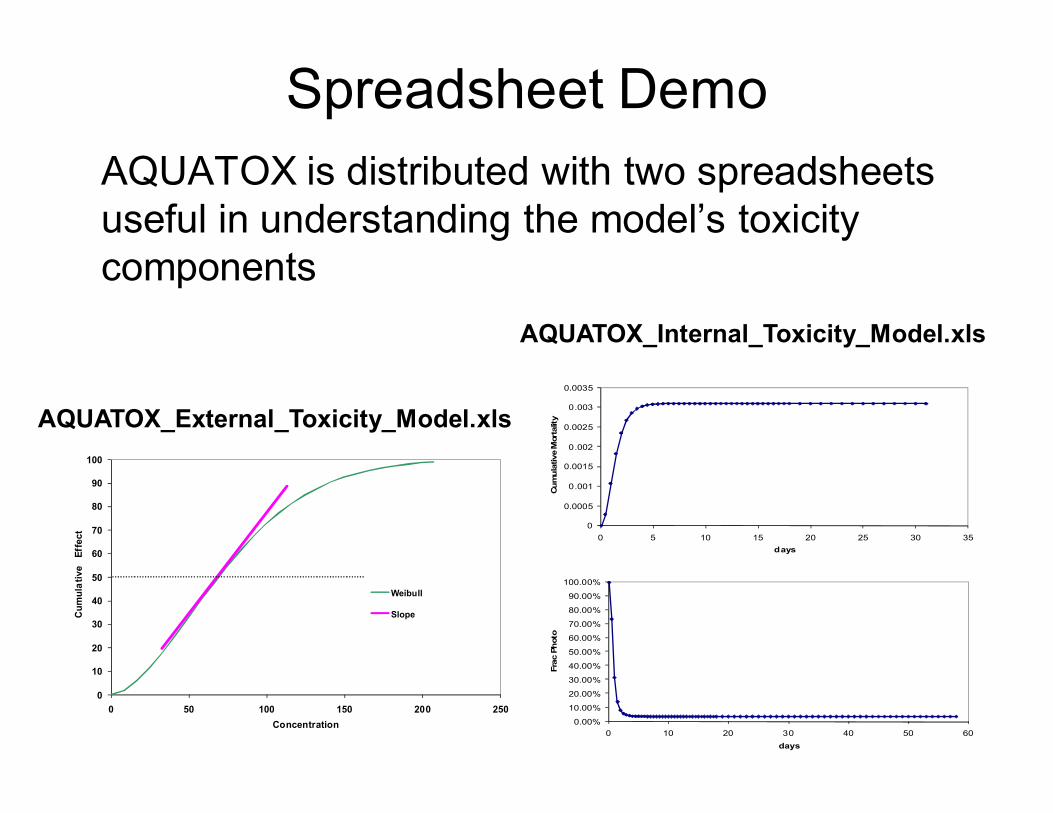
Spreadsheet Demo
AQUATOX is distributed with two spreadsheets useful in understanding the model’s toxicity components
0
10
20
30
40
50
60
70
80
90
100
0 50 100 150 200 250
Cu
mu
lati
ve
E
ffect
Concentration
Weibull
Slope
0
0.0005
0.001
0.0015
0.002
0.0025
0.003
0.0035
0 5 10 15 20 25 30 35
Cu
mu
lative M
ort
alit
ydays
0.00%
10.00%
20.00%
30.00%
40.00%
50.00%
60.00%
70.00%
80.00%
90.00%
100.00%
0 10 20 30 40 50 60
Fra
c P
hoto
days
AQUATOX_External_Toxicity_Model.xls
AQUATOX_Internal_Toxicity_Model.xls
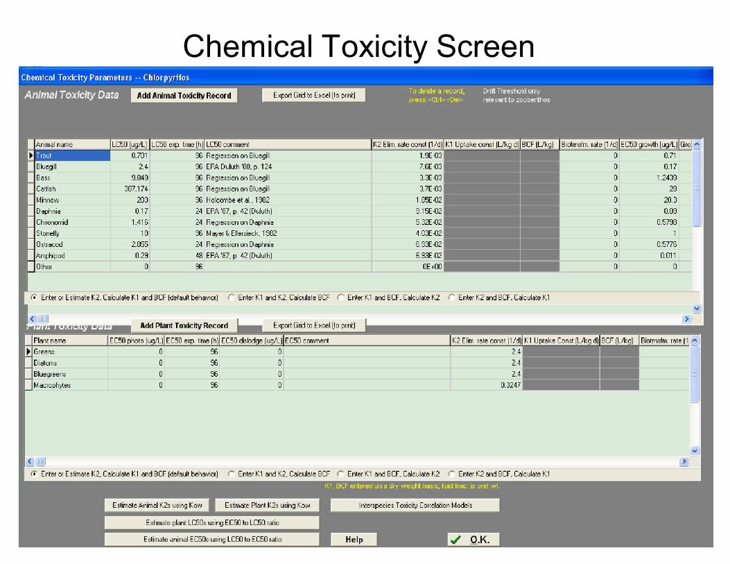
Chemical Toxicity Screen

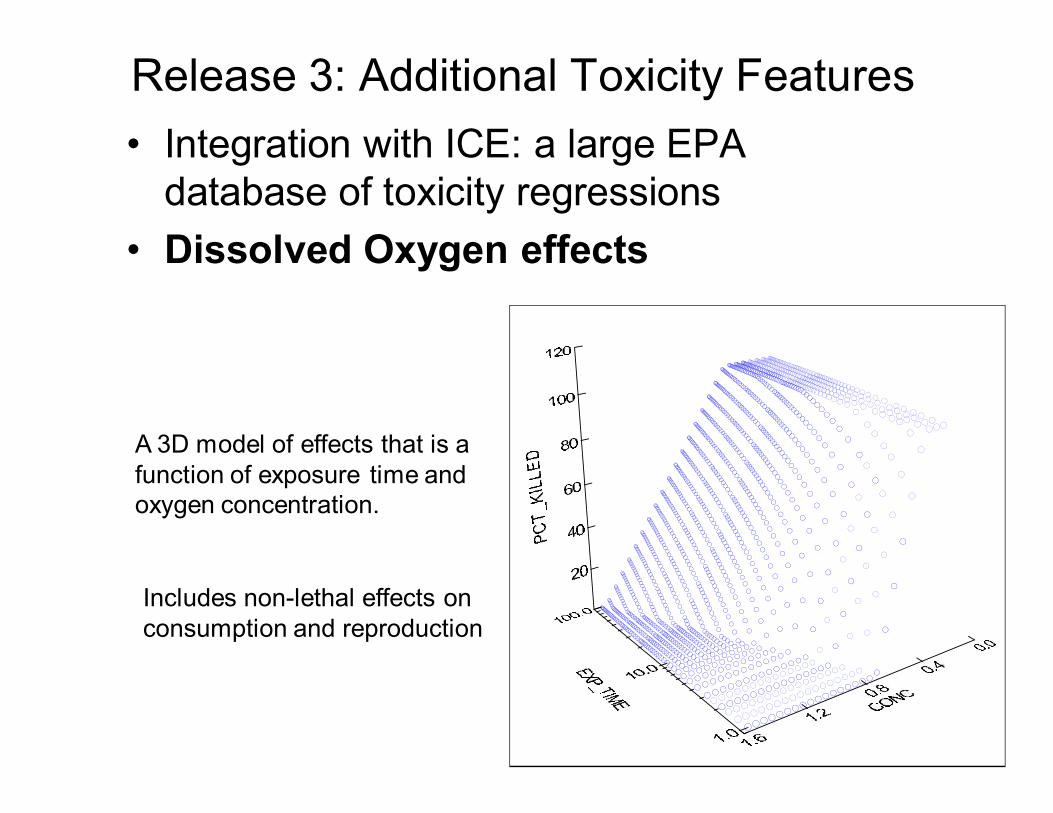
Release 3: Additional Toxicity Features
• Integration with ICE: a large EPA database of toxicity regressions
Release 3: Additional Toxicity Features
• Integration with ICE: a large EPA database of toxicity regressions
• Dissolved Oxygen effects
A 3D model of effects that is a function of exposure time and oxygen concentration.
Includes non-lethal effects on consumption and reproduction
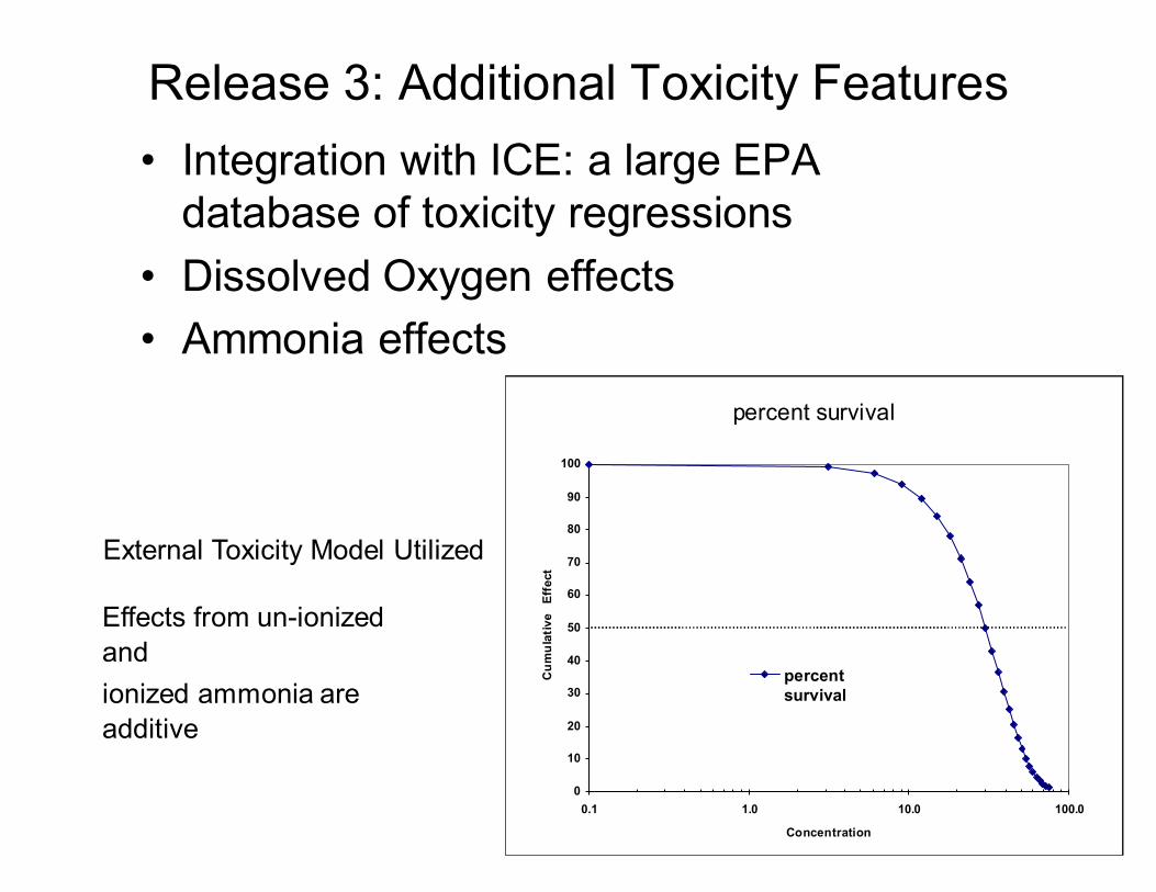
Release 3: Additional Toxicity Features
• Integration with ICE: a large EPA database of toxicity regressions
• Dissolved Oxygen effects
• Ammonia effects
percent survival
0
10
20
30
40
50
60
70
80
90
100
0.1 1.0 10.0 100.0
Concentration
Cu
mu
lati
ve
Eff
ect
percentsurvival
External Toxicity Model Utilized
Effects from un-ionized
and
ionized ammonia are
additive

Mussel NH3 Mort (Percent)
Mussel NH4+ Mort (Percent)
Mussel (g/m2 dry)
Cahaba River AL (CONTROL)Run on 10-29-08 4:53 PM
8/24/20022/23/20028/25/20012/24/2001
Perc
ent
1.1
1.0
0.9
0.8
0.7
0.6
0.5
0.4
0.3
0.2
0.1
0.0
g/m
2 d
ry
1.50
1.45
1.40
1.35
1.30
1.25
1.20
1.15
1.10
1.05
1.00Bluegill Low O2 Mort (Percent)
Bluegill NH3 Mort (Percent)
Bluegill NH4+ Mort (Percent)Bluegill Other Mort (Percent)
Bluegill Susp. Sed. Mort (Percent)
Bluegill (g/m2 dry)
Obs bluegill (g/m2 dry)
Cahaba River AL (CONTROL)Run on 10-29-08 4:53 PM
8/24/20022/23/20028/25/20012/24/20018/26/2000
Perc
ent
100
90
80
70
60
50
40
30
20
10
g/m
2 d
ry
0.27
0.24
0.21
0.18
0.15
0.12
0.09
0.06
0.03
0.00
Predicted ammonia toxicity in Cahaba River AL
1% mortality inmussels
100% mortalityIn bluegills

Returning to the Enclosure in Duluth MN . . .

Animals all decline at varying rates following a single initial dose of chlorpyrifos
Chironomid (g/m2 dry)
Green Sunfish, (g/m2 dry)
Shiner (g/m2 dry)
Green Sunfish2 (g/m2 dry)
Daphnia (mg/L dry)
CHLORPYRIFOS 6 ug/L (PERTURBED)Run on 11-7-08 11:36 AM
9/10/19868/26/19868/11/19867/27/19867/12/19866/27/1986
g/m
2 d
ry
0.36
0.32
0.28
0.24
0.20
0.16
0.12
0.08
0.04
0.00
mg/L d
ry
0.9
0.8
0.7
0.6
0.5
0.5
0.4
0.3
0.2
0.1
0.0
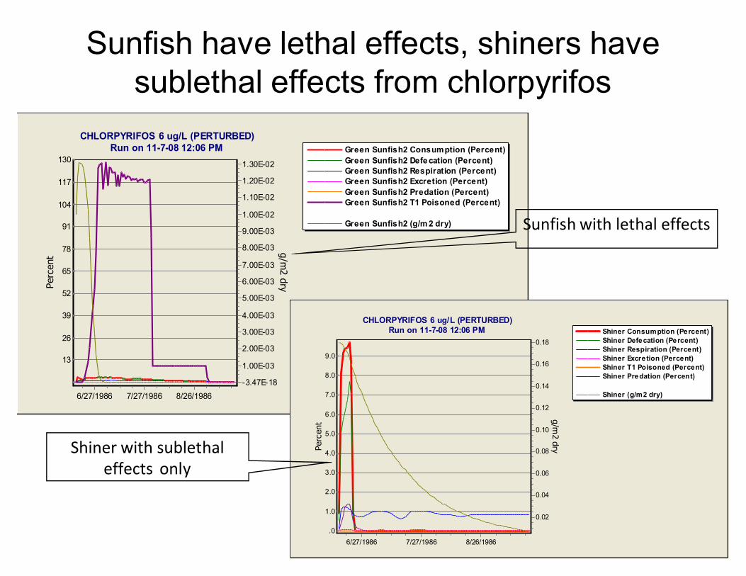
Sunfish have lethal effects, shiners have sublethal effects from chlorpyrifos
Green Sunfish2 Consumption (Percent)
Green Sunfish2 Defe cation (Percent)
Green Sunfish2 Respiration (Percent)
Green Sunfish2 Excretion (Percent)
Green Sunfish2 Predation (Percent)
Green Sunfish2 T1 Poisoned (Percent)
Green Sunfish2 (g/m 2 dry)
CHLORPYRIFOS 6 ug/L (PERTURBED)Run on 11-7-08 12:06 PM
8/26/19867/27/19866/27/1986
Perc
ent
130
117
104
91
78
65
52
39
26
13
g/m
2 d
ry
1.30E-02
1.20E-02
1.10E-02
1.00E-02
9.00E-03
8.00E-03
7.00E-03
6.00E-03
5.00E-03
4.00E-03
3.00E-03
2.00E-03
1.00E-03
-3.47E-18
Shiner Consumption (Percent)
Shiner Defecation (Percent)
Shiner Respiration (Percent)
Shiner Excretion (Percent)
Shiner T1 Poisoned (Percent)
Shiner Predation (Percent)
Shiner (g/m2 dry)
CHLORPYRIFOS 6 ug/L (PERTURBED)Run on 11-7-08 12:06 PM
8/26/19867/27/19866/27/1986
Perc
ent
9.0
8.0
7.0
6.0
5.0
4.0
3.0
2.0
1.0
.0
g/m
2 d
ry
0.18
0.16
0.14
0.12
0.10
0.08
0.06
0.04
0.02
Sunfish with lethal effects
Shiner with sublethal effects only
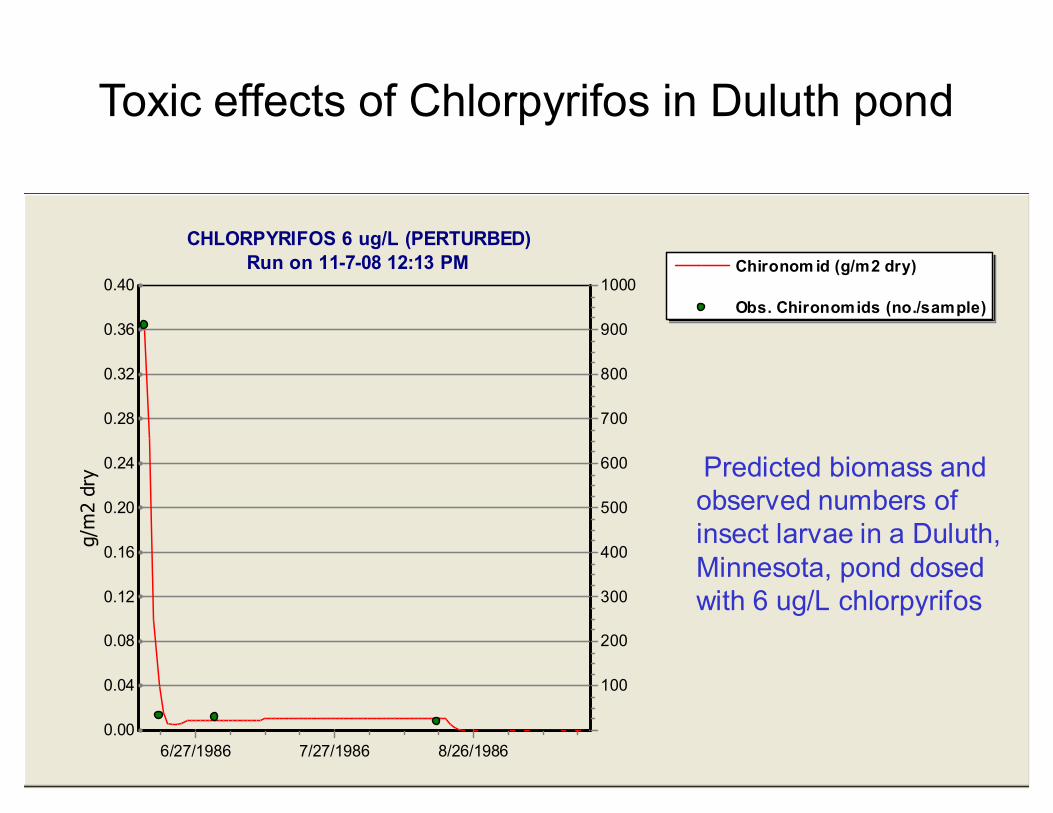
Chironom id (g/m2 dry)
Obs. Chironomids (no./sample)
CHLORPYRIFOS 6 ug/L (PERTURBED)Run on 11-7-08 12:13 PM
8/26/19867/27/19866/27/1986
g/m
2 d
ry
0.40
0.36
0.32
0.28
0.24
0.20
0.16
0.12
0.08
0.04
0.00
1000
900
800
700
600
500
400
300
200
100
Predicted biomass and observed numbers of insect larvae in a Duluth, Minnesota, pond dosed with 6 ug/L chlorpyrifos
Toxic effects of Chlorpyrifos in Duluth pond
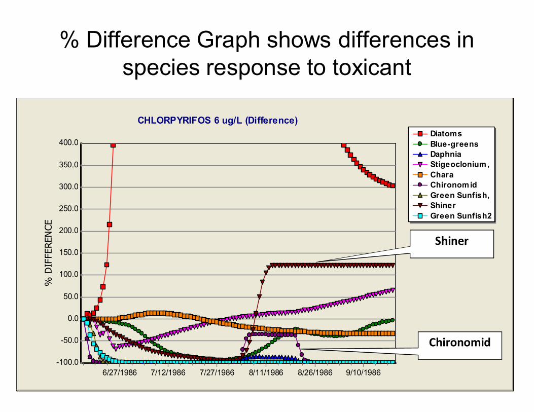
% Difference Graph shows differences in species response to toxicant
Diatoms
Blue-greens
Daphnia
Stigeoclonium,
Chara
Chironomid
Green Sunfish,
Shiner
Green Sunfish2
CHLORPYRIFOS 6 ug/L (Difference)
9/10/19868/26/19868/11/19867/27/19867/12/19866/27/1986
% D
IFFEREN
CE
400.0
350.0
300.0
250.0
200.0
150.0
100.0
50.0
0.0
-50.0
-100.0
Shiner
Chironomid

Steinhaus Indices show ecosystem impacts predicted by the model
n
kk
n
kk
n
kkk
aa
aaMin
S
1,2
1,1
1,2,1),(*2
Steinhaus Similarity Indices in Pond
0
0.2
0.4
0.6
0.8
1
1.2
6/16/
1986
6/23/
1986
6/30
/1986
7/7/
1986
7/14
/198
6
7/21
/198
6
7/28/
1986
8/4/1
986
8/11/
1986
8/18
/198
6
8/25/
1986
9/1/
1986
9/8/1
986
9/15/
1986
Plants
Invertebrates
Fish

Chlorpyrifos in Stream
Objective: analyze direct and indirect ecotoxicological effects with model
• Assessment of chlorpyrifos in a generic stream– small stream in corn belt
– exposure to constant level of Chlorpyrifos assessed (0.4 ug/L)
– optionally simulate with the initial condition of 0.4 ug/L as a one-time dose

Set exposure to a constant in Study SetupSet “Control Setup” to omit toxicants from “control” results
check box

Impacts of constant chlorpyrifos are dramatic: animals decline, algae increase (less herbivory)
Peri. Chlorophyll
ChironomidTubifex tubife
Mussel
Mayfly (Baetis
GastropodShiner
Yellow Perch
StonerollerWhite Sucker
Smallmouth Bas
Ohio Creek (Difference)
11/26/19979/27/19977/29/19975/30/19973/31/19971/30/1997
% D
IFFEREN
CE
400.0
350.0
300.0
250.0
200.0
150.0
100.0
50.0
0.0
-50.0
-100.0
periphyton
stoneroller
shinermayfly bass
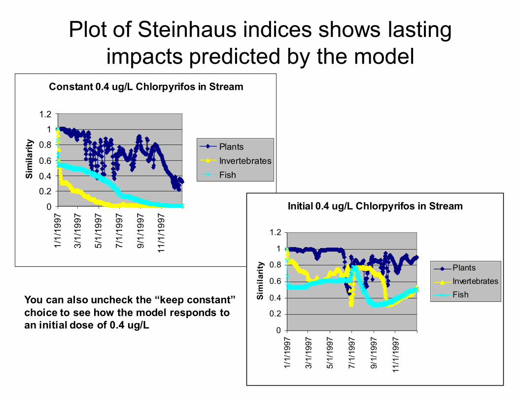
Constant 0.4 ug/L Chlorpyrifos in Stream
0
0.2
0.4
0.6
0.8
1
1.2
1/1
/19
97
3/1
/19
97
5/1
/19
97
7/1
/19
97
9/1
/19
97
11
/1/1
997
Sim
ila
rity Plants
Invertebrates
Fish
Plot of Steinhaus indices shows lasting impacts predicted by the model
Initial 0.4 ug/L Chlorpyrifos in Stream
0
0.2
0.4
0.6
0.8
1
1.2
1/1
/19
97
3/1
/19
97
5/1
/19
97
7/1
/19
97
9/1
/19
97
11
/1/1
99
7
Sim
ila
rity Plants
Invertebrates
FishYou can also uncheck the “keep constant”choice to see how the model responds to an initial dose of 0.4 ug/L

Farm Pond MO, Esfenvalerate
• Loadings from PRZM for adjacent cornfield
• Worst case scenario for runoff of pesticide predicted by PRZM
T1 H2O (ug/L)
FARM POND MO (PERTURBED)Run on 10-8-09 3:54 PM
4/11/19952/10/199512/12/199410/13/19948/14/19946/15/1994
ug/L
0.8
0.7
0.6
0.6
0.5
0.4
0.3
0.2
0.2
0.1
0.0
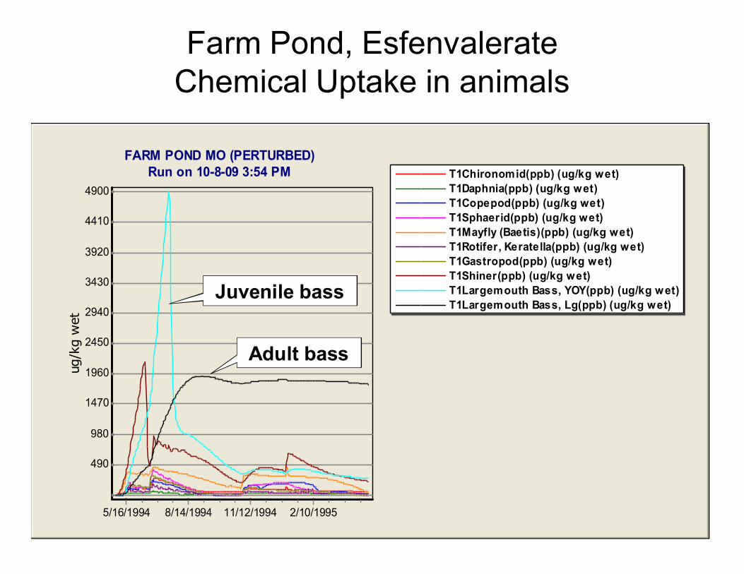
T1Chironomid(ppb) (ug/kg wet)
T1Daphnia(ppb) (ug/kg wet)
T1Copepod(ppb) (ug/kg wet)
T1Sphaerid(ppb) (ug/kg wet)
T1Mayfly (Baetis)(ppb) (ug/kg wet)
T1Rotifer, Keratella(ppb) (ug/kg wet)
T1Gastropod(ppb) (ug/kg wet)
T1Shiner(ppb) (ug/kg wet)
T1Largemouth Bass, YOY(ppb) (ug/kg wet)
T1Largemouth Bass, Lg(ppb) (ug/kg wet)
FARM POND MO (PERTURBED)Run on 10-8-09 3:54 PM
2/10/199511/12/19948/14/19945/16/1994
ug/k
g w
et
4900
4410
3920
3430
2940
2450
1960
1470
980
490
Farm Pond, Esfenvalerate Chemical Uptake in animals
Juvenile bass
Adult bass

Daphnia
Rotifer, Keratella
Mayfly (Baetis)
Gastropod
Shiner
Largemouth Bass, YOY
Largemouth Bass, Lg
Chironomid
FARM POND MO (Difference)
4/11/19952/10/199512/12/199410/13/19948/14/19946/15/1994
% D
IFFEREN
CE
100.0
80.0
60.0
40.0
20.0
0.0
-20.0
-40.0
-60.0
-80.0
-100.0
Farm Pond, EsfenvalerateDifference Graph
adult bass
rotifer
mayfly
snail

Fluridone (Sonar) used to eradicate Hydrilla in Clear Lake CA
• Six doses– 20 ppb dose
• What is impact on non-target organisms?
• What is recovery of
Clear Lake ecosystem?
• Impact on DO from death of large Hydrilla biomass?

T1 H2O (ug/L)
Hydrilla (g/m2 dry)
Largemouth Ba2 (g/m2 dry)
CLEAR LAKE, CA (PERTURBED) 7/8/2006 8:53:39 AM
1/14/19737/16/19721/16/19727/18/19711/17/19717/19/19701/18/1970
ug
/L
65
58
52
45
39
32
26
19
13
6
g/m
2 d
ry
10
9
8
7
6
5
4
3
2
1
Addition of Fluridone causes dramatic response of Clear Lake ecosystem
fluridone
Hydrilla
HydrillaCatfishLargemouth Ba2Bluegill
CLEAR LAKE, CA (Difference) 7/8/2006 8:58:13 AM
1/12/19737/14/19721/14/19727/16/19711/15/19717/17/19701/16/1970
% D
IFF
ER
EN
CE
400.0
350.0
300.0
250.0
200.0
150.0
100.0
50.0
0.0
-50.0
-100.0
bass

Indirect Effects Capturede.g. Impact on DO levels is negligible

Coralville Reservoir Iowa long-term contamination with dieldrin
• Run-of-river
• Flood control
• 90% of basin in
agriculture
– Nutrients
– Pesticides
– Sediment

Dieldrin bioaccumulates & declines over 20 yearswith fish mortality, but tolerant buffalofish, Tubifex prosper
T1Chironom id(ppb) (ug/kg wet)
T1Tubifex tubife(ppb) (ug/kg w et)
T1Daphnia(ppb) (ug/kg w et)
T1Predatory Zoop(ppb) (ug/kg w et)
T1Bluegill(ppb) (ug/kg w et)
T1Shad(ppb) (ug/kg wet)
T1Buffalofish22(ppb) (ug/kg w et)
T1Largem outh Ba2(ppb) (ug/kg w et)
T1Walleye(ppb) (ug/kg wet)
T1 H2O (ug/L)
CORALVILLE LAKE, IA (PERTURBED)
Run on 11-1-07 1:16 PM
12/12/197512/13/1971
ug/k
g w
et
1100
990
880
770
660
550
440
330
220
110
ug/L
0.036
0.032
0.028
0.024
0.020
0.016
0.012
0.008
0.004
0.000
Tubifex tubife
Bluegill
Shad
Buffalofish22
Largem outh Ba2
Walleye
CORALVILLE LAKE, IA (Difference) (Epilimnion Segment)
12/11/197712/12/197512/12/197312/13/197112/13/1969
% D
IFFEREN
CE
400.0
350.0
300.0
250.0
200.0
150.0
100.0
50.0
0.0
-50.0
-100.0
Shad, bluegill, walleye,bass die off
Walleye startto recover
Buffalofish & Tubifex
Dieldrin, dissolved

BluegillBuffalofish22Largemouth BasWalleye
Biomass Risk Graph
11/9/2008 9:13:08 AM
Percent Decline at Simulation End
1009080706050403020
Pe
rce
nt
Pro
ba
bilit
y
100.0
90.0
80.0
70.0
60.0
50.0
40.0
30.0
20.0
Probability of decline in biomass (end of 1st year) can be estimated based on uncertainty
Buffalofish tolerant
100% probability that juv.bass will decline 89%
Bluegill moresensitive
60% probability thatwalleye will decline 61%

Uncertainty and Sensitivity Analysis
• “Sensitivity” refers to the variation in output of a mathematical model with respect to changes in the values of the model inputs (Saltelli, 2001).
• Sensitivity analysis provides a ranking of the model input assumptions with respect to their relative contribution to model output variability or uncertainty (EPA, 1997).
• A comprehensive sensitivity analysis of AQUATOX has been performed for diverse sites.

Coralville Sensitivity Analysis Demo
Demonstration of inputs and outputs from Coralville analysis
Sensitivity of Tubifex tubife (g/m2 dry) to 20% change in tested parameters3/28/2008 3:31:16 PM
Tubifex tubife (g/m2 dry)
20191817161514131211
5.45% - Daphnia: Maximum Temperature (deg. C)
6.82% - Susp&Diss Detr: Multiply Loading by
12.6% - Daphnia: Temperature Response Slope
13.1% - Cyclotella nan: Maximum Temperature (deg. C)
16.3% - Daphnia: Max Consumption (g / g day)
16.5% - Cyclotella nan Min. Sat. Light (Ly/d)
19.7% - Daphnia: Optimal Temperature (deg. C)
23.1% - Water Vol: Multiply Loading by
40.8% - Cyclotella nan: Temp Response Slope
51.2% - Cyclotella nan: Optimal Temperature (deg. C)
62.4% - Cyclotella nan: Max Photosynthetic Rate (1/d)
66.6% - TSS: Multiply Loading by
83.2% - Water Vol: Mult. Inflow Load by
135% - Temp: Multiply Loading by

Uncertainty Analysis
• Uncertainty analyses describe sources of incertitude and variability
• There are many sources of uncertainty e.g.– parameter uncertainty
– model uncertainty due to necessary simplification of real-world processes
• Monte Carlo analysis is a statistical sampling technique that allows us to obtain a probabilistic approximation to the effects of parameter uncertainty
• AQUATOX Utilizes Monte Carlo analysis with efficient “Latin Hypercube Sampling” (greatly reduces required iterations)
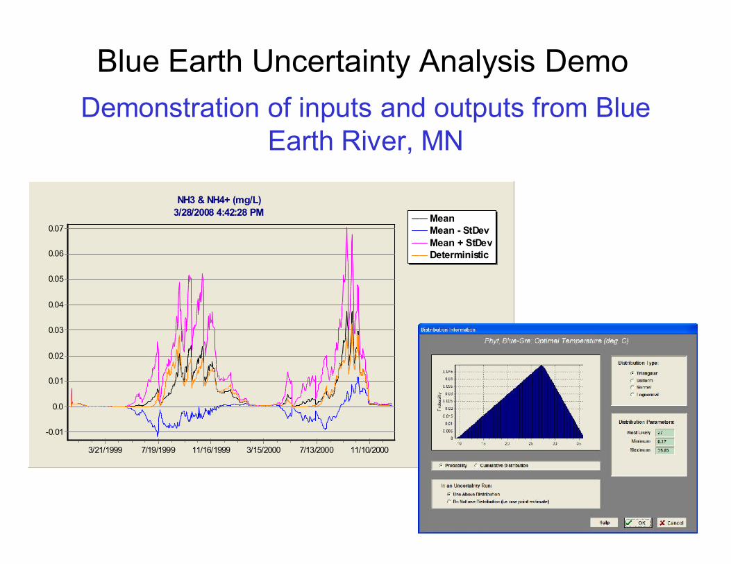
Blue Earth Uncertainty Analysis Demo
Demonstration of inputs and outputs from Blue Earth River, MN
MeanMean - StDev
Mean + StDevDeterministic
NH3 & NH4+ (mg/L)
3/28/2008 4:42:28 PM
11/10/20007/13/20003/15/200011/16/19997/19/19993/21/1999
0.07
0.06
0.05
0.04
0.03
0.02
0.01
0.0
-0.01

Sediment Effects Overview
• Suspended and bedded sediment effects
– Mortality
• Highly Sensitive
• Sensitive
• Intolerant
• Tolerant
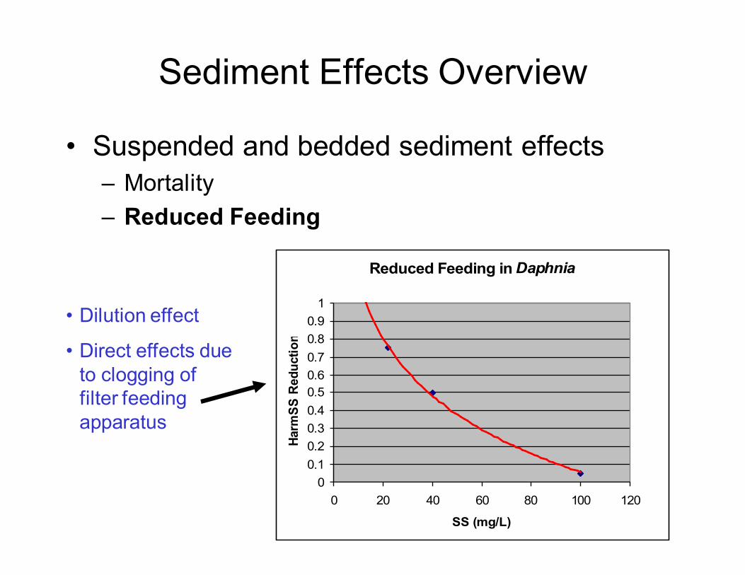
Sediment Effects Overview
• Suspended and bedded sediment effects
– Mortality
– Reduced Feeding
Reduced Feeding in Daphnia
0
0.1
0.2
0.3
0.4
0.5
0.6
0.7
0.8
0.9
1
0 20 40 60 80 100 120
SS (mg/L)
Harm
SS
Re
du
cti
on
• Dilution effect
• Direct effects due to clogging of filter feeding apparatus
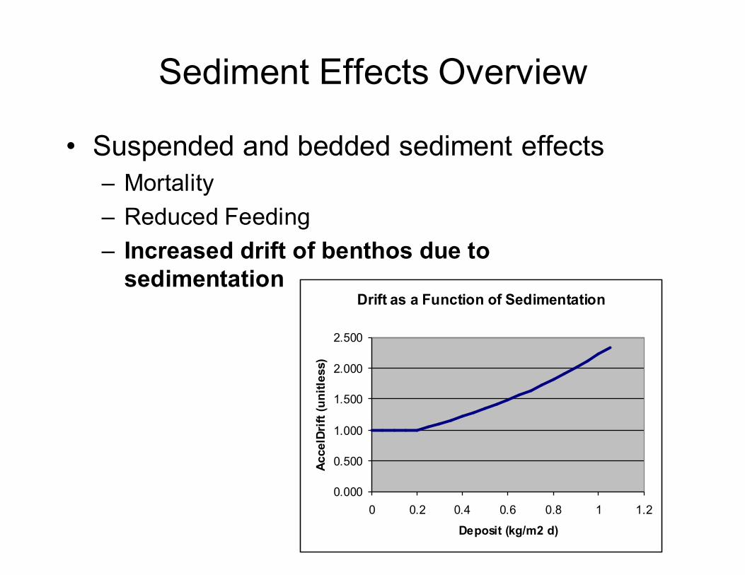
Sediment Effects Overview
• Suspended and bedded sediment effects
– Mortality
– Reduced Feeding
– Increased drift of benthos due to sedimentation
Drift as a Function of Sedimentation
0.000
0.500
1.000
1.500
2.000
2.500
0 0.2 0.4 0.6 0.8 1 1.2
Deposit (kg/m2 d)
AccelD
rift
(u
nit
less)
Sediment Effects Overview
• Suspended and bedded sediment effects
– Mortality
– Reduced Feeding
– Increased drifting of grazers due to sedimentation
– Deposition of fines and their effect on invertebrates and salmonid reproduction
• Percent Embeddedness calculated as a function of 60-day average TSS

Percent embeddedness is computed from 60-day deposition rate (a function of TSS)
Pct. Embeddedness (percent)
60-day avg. Inorg. Sed. (m g/L)
Blue Earth River MN (CONTROL)Run on 10-31-08 4:48 PM
8/26/20002/26/20008/28/19992/27/1999
perc
ent
37
33
30
26
22
19
15
11
7
4
mg/L
165.0
150.0
135.0
120.0
105.0
90.0
75.0
60.0
45.0
30.0

Mayflies, stoneflies, & caddisflies (EPT) are sensitive to embeddedness; chironomids & oligochaetes are not
Percent EPT (percent)
Percent Chironom id (percent)
Tubifex tubife (g/m2 dry)
Blue Earth River MN (CONTROL)Run on 10-31-08 4:48 PM
8/26/20002/26/20008/28/19992/27/1999
perc
ent
4.5
4.0
3.5
3.0
2.5
2.0
1.5
1.0
.5
.0
g/m
2 d
ry
6.0
5.4
4.8
4.2
3.6
3.0
2.4
1.8
1.2
.6
.0

Doubling TSS increases embeddedness in Cahaba River, AL
Pct. Embeddedness (percent)
Inorg. Deposition (kg/m2 d)
Cahaba River AL (CONTROL)Run on 10-31-08 4:58 PM
8/24/20022/23/20028/25/20012/24/2001
perc
ent
28.0
26.6
25.2
23.8
22.4
21.0
19.6
18.2
16.8
15.4
kg/m
2 d
1.0
0.9
0.8
0.7
0.6
0.5
0.4
0.3
0.2
0.1
0.0
Pct. Embeddedness (percent)
Inorg. Deposition (kg/m2 d)
Cahaba River AL (PERTURBED)Run on 10-31-08 6:02 PM
8/24/20022/23/20028/25/20012/24/2001
perc
ent
28.0
26.6
25.2
23.8
22.4
21.0
19.6
18.2
16.8
15.4
kg/m
2 d
1.0
0.9
0.8
0.7
0.6
0.5
0.4
0.3
0.2
0.1
0.0
control
X2 TSS

Doubling TSS loadings adversely impacts insect community in Cahaba River, AL
Percent EPT (percent)
Mayfly (Baetis (g/m2 dry)Stonefly (g/m2 dry)
Cahaba River AL (CONTROL)Run on 10-31-08 4:58 PM
8/24/20022/23/20028/25/20012/24/2001
perc
ent
1.2
1.1
1.0
0.9
0.8
0.7
0.6
0.5
0.4
0.3
0.2
0.1
g/m
2 d
ry
0.11
0.10
0.09
0.08
0.07
0.06
0.05
0.04
0.03
0.02
0.01
0.00 Percent EPT (percent)
Mayfly (Bae tis (g/m2 dry)Stonefly (g/m2 dry)
Cahaba River AL (PERTURBED)Run on 10-31-08 6:02 PM
8/24/20022/23/20028/25/20012/24/2001
perc
ent
1.2
1.1
1.0
0.9
0.8
0.7
0.6
0.5
0.4
0.3
0.2
0.1
g/m
2 d
ry
0.11
0.10
0.09
0.08
0.07
0.06
0.05
0.04
0.03
0.02
0.01
0.00
control
X2 TSS
stoneflies crash

Closure
• Topics not yet covered (time-permitting)
– Diel Oxygen
– Sand-Silt-Clay model
– Multi-layer sediment model
• Final Q&A

Please Keep in Touch!
• Applications help drive enhancements, example studies and data libraries
• Growing user community builds robustness and confidence
• Continued model and user support
– One-on-one technical support is available
– AQUATOX listserver
• Visit the AQUATOX web site
– http://water.epa.gov/scitech/datait/models/aquatox/index.cfm
– Citations of articles using or reviewing AQUATOX
– Data sources

Diel Oxygen, Light; Hourly time-step
Peri Low-Nut D (g/sq.m)
Peri High-Nut (g/sq.m)
Peri, Nitzschi (g/sq.m)
Cladophora (g/sq.m)
Peri, Green (g/sq.m)
Peri, Blue-Gre (g/sq.m)
Fontinalis (g/sq.m)
Oxygen (mg/L)
Rum R. 18 MN (PERTURBED) 7/7/2005 2:03:26 PM
(Epilimnion Segment)
10/1/20009/16/20009/1/20008/17/20008/2/2000
g/s
q.m 1.0
0.0
mg
/L
12.0
11.0
10.0
9.0
8.0
Monitoring data indicate that oxygen levels fluctuate daily
AQUATOX can now run with an hourly time-step including hourly light inputs. This results in a simulation of oxygenconcentrations on an hourly basis

Diel Oxygen, Hourly Time-step
Oxygen (mg/L)
Min. Oxygen (mg/L)
Max. Oxygen (mg/L)
Obs DO at Glenwood (m g/L)DO at GB, City of Boise (mg/L)
Obs DO Glenwood (mg/L)
Seg 3 (PERTURBED)Run on 09-2-07 4:58 PM
12/3/200511/26/200511/19/2005
mg/L
15.3
14.4
13.5
12.6
11.7
10.8
9.9
9.0
8.1
7.2

Modeling Inorganic Sediments(sand, silt, and clay)
• Stream simulations only
• Scour, deposition and transport of sediments
• River reach assumed short and well mixed
• Daily average flow regime determines shear stresses
• Feedback to biota through light limitation, sequestration of chemicals, and now direct sediment effects

Critical Shear Stress for Erosion and Deposition Key Parameters
Tau Erosion
Tau Deposition
Critica
l Shear
Str
ess
for
Site (
kg/m
2)
Net Deposition Net Erosion
(bed is stable)

To
x
g
/Lp
w
DOM in Water Col. mg/Lwc
To
x
g
/Lw
c
To
x
g
/Lp
w
Susp. Detr mg/L
To
x
g
/ Lw
c
Sed Detr mg/L
Wate
r Colu
mn
Laye
r 1Laye
r 2Laye
r n
Buried Detr g/m2
Buried Detr g/m2
To
x
g
/ Lw
c
To
x
g
/ m2
To
x
g
/ m2
Water Col. m3
To
x
g
/Lw
c
To
x
g / L
wc
Susp. Inorg.
Solids mg/Lwc
Inorganic Solids g/m2
To
x
g/ m
2
Pore Water m3/m2
DOM in Pore
Water mg/Lpw
Inorganic
Solids g/m2
To
x
g/ m
2
Inorganic
Solids g/m2
To
x
g/ m
2
To
x
g
/Lpw
DOM in Pore
Water mg/Lpw
To
x
g
/Lp
w
DOM in Pore
Water mg/Lpw
To
x
g
/Lp
w
Pore Water m3/m2
To
x
g
/Lp
w
Pore Water m3/m2
AQUATOX Multi-Layer Sediment Model based on the IPX module (Velleux et al. 2000)


