
Water Research 38 (2004) 1305–1317
ARTICLE IN PRESS
*Correspond
2559-5337.
E-mail addr
0043-1354/$ - se
doi:10.1016/j.w
Modelling particle size distribution dynamics in marine waters
Xiao-yan Li*, Jian-jun Zhang, Joseph H.W. Lee
Department of Civil Engineering, Environmental Engineering Research Centre, The University of Hong Kong,
Pokfulam Road, Hong Kong, China
Received 4 June 2003; received in revised form 31 October 2003; accepted 7 November 2003
Abstract
Numerical simulations were carried out to determine the particle size distribution (PSD) in marine waters by
accounting for particle influx, coagulation, sedimentation and breakage. Instead of the conventional rectilinear model
and Euclidean geometry, a curvilinear collision model and fractal scaling mathematics were used in the models. A
steady-state PSD can be achieved after a period of simulation regardless of the initial conditions. The cumulative PSD
in the steady state follows a power-law function, which has three linear regions after log–log transformation, with
different slopes corresponding to the three collision mechanisms, Brownian motion, fluid shear and differential
sedimentation. The PSD slope varies from �3.5 to �1.2 as a function of the size range and the fractal dimension of the
particles concerned. The environmental conditions do not significantly alter the PSD slope, although they may change
the position of the PSD and related particle concentrations. The simulation demonstrates a generality in the shape of
the steady-state PSD in the ocean, which is in agreement with many field observations. Breakage does not affect the size
distribution of small particles, while a strong shear may cause a notable change in the PSD for larger and fractal
particles only. The simplified approach of previous works using dimensional analysis still offers valuable
approximations for the PSD slopes, although the previous solutions do not always agree with the simulation results.
The variation in the PSD slope observed in field investigations can be reproduced numerically. It is argued that non-
steady-state conditions in natural waters could be the main reason for the deviation of PSD slopes. A change in the
nature of the particles, such as stickiness, and environmental variables, such as particle input and shear intensity, could
force the PSD to shift from one steady state to another. During such a transition, the PSD slope may vary to some
extent with the particle population dynamics.
r 2003 Elsevier Ltd. All rights reserved.
Keywords: Coagulation; Flocculation; Fractal; Marine water; Particle; Particle size distribution (PSD); Phytoplankton bloom
1. Introduction
Particulate materials in the ocean play an important
role in the transport of many substances, including
biogenic matter, trace metals and organic pollutants,
from surface waters to, eventually, the ocean floor.
Natural particles can vary widely in size from sub-
micron colloids to larger aggregates of a few millimetres,
such as marine snow. Field observations indicate that
the particle population in marine waters has a size
ing author. Tel.: +852-2859-2659; fax: +852-
ess: [email protected] (X.-Y. Li).
e front matter r 2003 Elsevier Ltd. All rights reserve
atres.2003.11.010
distribution that may be fitted by a power-law function,
i.e., NðlÞBl�b; where NðlÞ is the cumulative number
concentration of particles of size l or larger, and �b is
defined as the slope of the size distribution [1–7]. Despite
vast differences in particle properties and environmental
conditions in different waters, the size distribution
slopes are found to vary within a narrow range only,
which is mainly from �1.5 to �4.0, particularly for
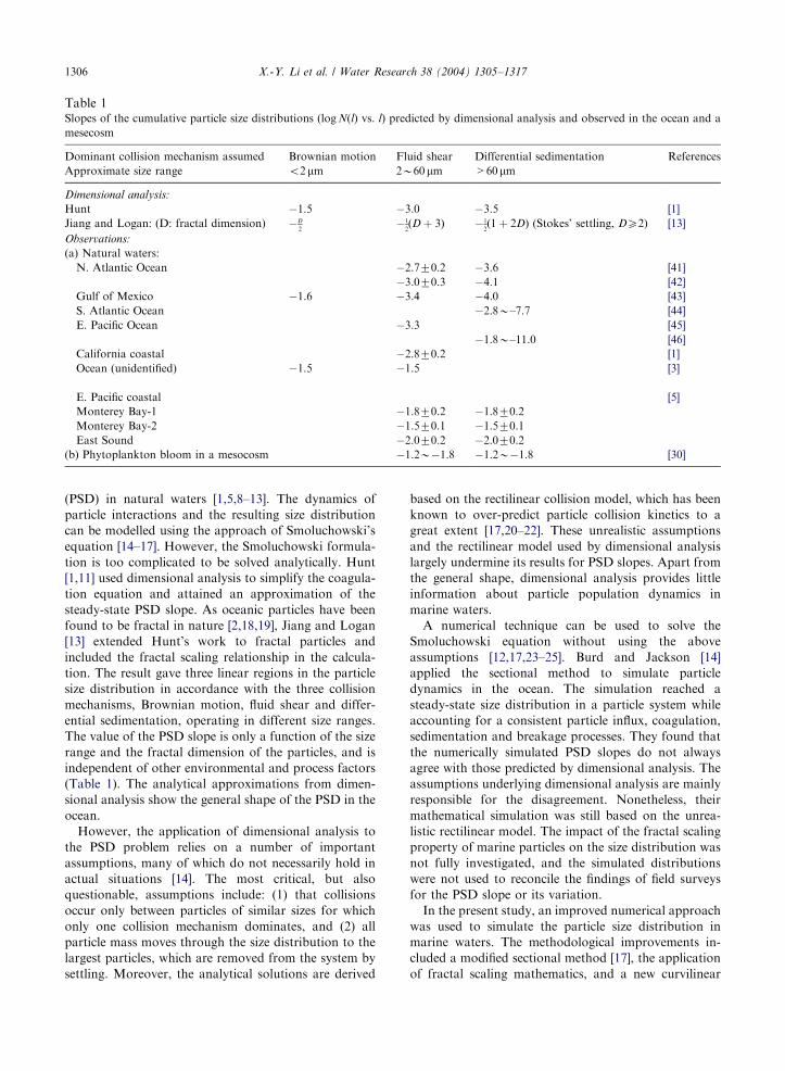
particles smaller than 100mm (Table 1). Field observa-
tions suggest a generality in the shape of the size
distribution of marine particles, which, however, re-
mains to be established theoretically.
Particle coagulation has been considered to play a
major role in determining the particle size distribution
d.
ARTICLE IN PRESS
Table 1Slopes of the cumulative particle size distributions (logN(l) vs. l) predicted by dimensional analysis and observed in the ocean and a
mesecosm
Dominant collision mechanism assumed Brownian motion Fluid shear Differential sedimentation References
Approximate size range o2 mm 2B60 mm >60mm
Dimensional analysis:
Hunt �1.5 �3.0 �3.5 [1]
Jiang and Logan: (D: fractal dimension) �D
2�1
2ðD þ 3Þ �1
2ð1þ 2DÞ (Stokes’ settling, DX2) [13]
Observations:
(a) Natural waters:
N. Atlantic Ocean �2.770.2 �3.6 [41]
�3.070.3 �4.1 [42]
Gulf of Mexico �1.6 �3.4 �4.0 [43]
S. Atlantic Ocean �2.8B–7.7 [44]
E. Pacific Ocean �3.3 [45]
�1.8B–11.0 [46]
California coastal �2.870.2 [1]
Ocean (unidentified) �1.5 �1.5 [3]
E. Pacific coastal [5]
Monterey Bay-1 �1.870.2 �1.870.2
Monterey Bay-2 �1.570.1 �1.570.1
East Sound �2.070.2 �2.070.2
(b) Phytoplankton bloom in a mesocosm �1.2B�1.8 �1.2B�1.8 [30]
X.-Y. Li et al. / Water Research 38 (2004) 1305–13171306
(PSD) in natural waters [1,5,8–13]. The dynamics of
particle interactions and the resulting size distribution
can be modelled using the approach of Smoluchowski’s
equation [14–17]. However, the Smoluchowski formula-
tion is too complicated to be solved analytically. Hunt
[1,11] used dimensional analysis to simplify the coagula-
tion equation and attained an approximation of the
steady-state PSD slope. As oceanic particles have been
found to be fractal in nature [2,18,19], Jiang and Logan
[13] extended Hunt’s work to fractal particles and
included the fractal scaling relationship in the calcula-
tion. The result gave three linear regions in the particle
size distribution in accordance with the three collision
mechanisms, Brownian motion, fluid shear and differ-
ential sedimentation, operating in different size ranges.
The value of the PSD slope is only a function of the size
range and the fractal dimension of the particles, and is
independent of other environmental and process factors
(Table 1). The analytical approximations from dimen-
sional analysis show the general shape of the PSD in the
ocean.
However, the application of dimensional analysis to
the PSD problem relies on a number of important
assumptions, many of which do not necessarily hold in
actual situations [14]. The most critical, but also
questionable, assumptions include: (1) that collisions
occur only between particles of similar sizes for which
only one collision mechanism dominates, and (2) all
particle mass moves through the size distribution to the
largest particles, which are removed from the system by
settling. Moreover, the analytical solutions are derived
based on the rectilinear collision model, which has been
known to over-predict particle collision kinetics to a
great extent [17,20–22]. These unrealistic assumptions
and the rectilinear model used by dimensional analysis
largely undermine its results for PSD slopes. Apart from
the general shape, dimensional analysis provides little
information about particle population dynamics in
marine waters.
A numerical technique can be used to solve the
Smoluchowski equation without using the above
assumptions [12,17,23–25]. Burd and Jackson [14]
applied the sectional method to simulate particle
dynamics in the ocean. The simulation reached a
steady-state size distribution in a particle system while
accounting for a consistent particle influx, coagulation,
sedimentation and breakage processes. They found that
the numerically simulated PSD slopes do not always
agree with those predicted by dimensional analysis. The
assumptions underlying dimensional analysis are mainly
responsible for the disagreement. Nonetheless, their
mathematical simulation was still based on the unrea-
listic rectilinear model. The impact of the fractal scaling
property of marine particles on the size distribution was
not fully investigated, and the simulated distributions
were not used to reconcile the findings of field surveys
for the PSD slope or its variation.
In the present study, an improved numerical approach
was used to simulate the particle size distribution in
marine waters. The methodological improvements in-
cluded a modified sectional method [17], the application
of fractal scaling mathematics, and a new curvilinear

ARTICLE IN PRESSX.-Y. Li et al. / Water Research 38 (2004) 1305–1317 1307
collision model developed by Han and Lawler [20]. The
simulation results were compared with the previous
dimensional analysis and field observations of the shape
of particle size distributions. The generality of marine
PSD was verified in terms of the slope values. In
addition, a simulation of the transition between the
status of different steady states and related particle
population dynamics helped to explain the variation in
the slope values observed in the field.
2. Theory and methods
2.1. Flocculation equation
The flocculation process in a system of heterodisperse
particles has been modelled by the change in particle size
distribution [14,23,24,26–28]. When simultaneous ac-
tions of particle influx, coagulation, sedimentation and
breakage are considered, the particle size distribution
dynamics can be described in the form of the Smo-
luchowski equation given below:
dnðmÞdt
¼ 12
Z m
0
abðm � m0;m0Þnðm � m0Þnðm0Þ dm0
� nðmÞZ
N
0
abðm;m0Þnðm0Þ dm0
� sðmÞnðmÞ þZ
N
m
gðm;m00Þsðm00Þnðm00Þ dm00
�uðmÞ
HnðmÞ þ fðmÞ; ð1Þ
where t is time, nðmÞ is the particle size density function
with respect to the particle size measured by mass, m;m0
is the mass of another particle, which is smaller than m
in the first term on the right-hand side of the equation, bis the collision frequency function describing the rate of
contacts between the particles indicated, a is the collisionefficiency defined as fraction of collisions that result in
particle attachment, sðmÞ is the break-up rate function,
gðm;m00Þ is the breakage distribution function defining
the mass fraction of fragments of size m breaking from a
larger aggregate of size m00;H is the depth of the water
column, uðmÞ is the settling velocity and fðmÞ is the
input rate of the particles concerned.
The sectional approximation has been employed to
find numerical solutions to Eq. (1). Following the
common approach of the sectional method
[12,16,17,23], the size sections are so generated that the
upper bound of a section is twice its lower bound in
terms of mass, e.g., mk ¼ 2mk�1 for section k: Within
each size section, it is assumed here that the particle
mass is distributed uniformly along the log-scale, which
gives a particle size density function of nðmÞ ¼Qk=ððln 2Þm2Þ; where Qk is the particle mass concentra-
tion in the kth section [17]. Subsequently, Eq. (1) can be
converted to
dQk
dt¼Qk�1
Xk�1
i¼1
1Bi;k�1;kQi þ Qk
Xk
i¼1
2Bi;k;kQi
� Qk
Xk
i¼1
3Bi;k;kQi � 4Bk;k;kQ2k � Qk
Xs
i¼kþ1
5Bk;i;kQi
� 1SkQk þXs
i¼kþ1
2Sk;iQi � UkQk þ qk; ð2Þ
where i signifies the section number and s is the last size
section. Eq. (2) is the governing equation for modelling
particle size dynamics in an open system, such as marine
waters. For any given section, such as section k; there isa total of nine cases of particle input, attachment,
breakage and sedimentation involved in the mass
movement. Table 2 illustrates the nine particle transport
and transformation processes that result in the gain and
loss of particle mass in the kth section.1Bi;k�1;k; 2Bi;k;k; 3Bi;k;k; 4Bk;k;k and 5Bk;i;k are the sec-
tional coagulation coefficients, 1Sk and 2Sk;i are the
sectional breakage coefficients, Uk is the sectional
settling velocity and qk is the sectional particle input
rate. The computation of these sectional coefficients is
also summarized in Table 2. Eq. (2) represents a finite
number of coupled ordinary differential equations for
the change in particle concentrations in all the size
sections. These differential equations can readily be
solved using the fourth-order Runge–Kutta method
with a constant time step of 1 s, as described elsewhere
[17,28].
2.2. Fractal aggregates
Although mass is used to track particle transport
between size sections, the rates of particle coagulation
and breakup depend more directly on the actual length
of the particles. Natural particles have been character-
ized as fractals with a highly porous and amorphous
structure [2,5,13,18,29]. For fractal particles, the length,
l; can be related to the mass by mBlD; or
l ¼ cm
rp
!1=D
; ð3Þ
where rp is the density of primary particles and c is an
empirical constant [13,30]. The settling velocity of a
fractal particle can be calculated using Stokes’ law, or
uðmÞ ¼gðrp � rlÞm
3pmrpl; ð4Þ
where g is the gravitational constant, rl is the density
and m is the viscosity of the liquid [31,32].

ARTIC
LEIN
PRES
STable 2Different particle transport cases and related sectional rate coefficients
Case Symbol Description Illustration Calculation f ðmx;myÞ ¼
ðabðmx;myÞÞ=ððln 2Þ2m2xm2
yÞ
1 Gain 1Bi;j;k Newly formed doublet moving into the kth section
ðmk�1oðmx þ myÞomkÞ; m0pmxpmk�1 and
mk�2pmyomk�1; ipk � 1; j ¼ k � 1:
R mi
mi�1
R mk�1
mk�1�mxðmx þ myÞf ðmx;myÞ dmx dmy
1
2
R mk�1
mk�2
R mk�1
mk�2ðmx þ myÞf ðmx;myÞ dmx dmy
2 Gain 2Bi;j;k Newly formed doublet in the kth section ðmk�1oðmx þmyÞomkÞ; m0pmxomk�1 and mk�1pmyomk; iok; j ¼ k:
R mi
mi�1
R mk�mx
mk�1mxf ðmx;myÞ dmx dmy
3 Loss 3Bi;j;k A particle being moved out of the kth section by
attachment to a smaller particle ðmkoðmx þmyÞÞ; m0pmxomk�1 and mk�1pmyomk; iok; j ¼ k:
R mi
mi�1
R mk�mx
mk�1myf ðmx;myÞ dmx dmy
4 Loss 4Bi;j;k A particle being moved out of the kth section by
attachment to a similarly sized particle; ðmkoðmx þmyÞÞ; mk�1pmxomk and mk�1pmyomk; i ¼ k; j ¼ k:
1
2
R mk
mk�1
R mk
mk�1ðmx þ myÞf ðmx;myÞ dmx dmy
5 Loss 5Bk;i;j A particle being moved out of the kth section by
attachment to a larger particle ðmkoðmx þmyÞÞ; mk�1pmxomk and mkpmy; i ¼ k; j > k
R mk
mk�1
R mj
mj�1myf ðmx;myÞ dmx dmy
6 Loss 1Sk Particles being moved out of the kth section by breakage,
mk�1omomk :
R mk
mk�1
sðmÞm ln2
dm
7 Gain 2Sk;i Particle fragments moving into the kth section by breakage
of larger particles, mk�1omomk and mi�1omzomi; koi:
R mk
mk�1
R mi
mi�1
gðm;mzÞsðmzÞmz ln2
dmz dm
8 Loss Uk Particles moving out of the kth section by sedimentation,
mk�1omomk :
R mk
mk�1
uðmÞH � m ln2
dm
9 Gain Qk Particles inputting into the kth section, mk�1omomk:R mk
mk�1fðmÞm dm
X.-Y
.L
iet
al.
/W
ater
Resea
rch3
8(
20
04
)1
30
5–
13
17
1308

ARTICLE IN PRESSX.-Y. Li et al. / Water Research 38 (2004) 1305–1317 1309
2.3. Coagulation models
The rectilinear collision model, which assumes that
particles move in straight lines until a collision occurs,
has the following formulations for the collision fre-
quency functions of the three collision mechanisms.
Brownian motion:
bBrði; jÞ ¼2kT
3m1
liþ
1
lj
� �ðli þ ljÞ: ð5aÞ
Fluid shear:
bShði; jÞ ¼G
6ðli þ ljÞ
3: ð5bÞ
Differential sedimentation:
bDSði; jÞ ¼p4ðli þ ljÞ
2 ui � uj
�� ��; ð5cÞ
where k is Boltzmann’s constant, T is the absolute
temperature, and G is the shear rate which is a
measurement of the turbulence intensity in water. The
total interparticle collision frequency function is the sum
of these three independent mechanisms, i.e.,
bði; jÞ ¼ bBrði; jÞ þ bShði; jÞ þ bDSði; jÞ: ð6Þ
The curvilinear collision model takes into account
hydrodynamic interactions and short-range forces be-
tween approaching particles, which results in reduced,
but more realistic, collision frequencies between im-
permeable particles [20,21,33,34]. According to Han and
Lawler [20], the curvilinear bcur can be related to the
well-defined rectilinear b by the reduction factors, i.e.,
bcurði; jÞ ¼ eBrbBrði; jÞ þ eShbShði; jÞ þ eDSbDSði; jÞ; ð7Þ
where eBr; eSh and eDS are the curvilinear reduction
factors for the collision mechanisms indicated. Based on
their numerical solutions, Han and Lawler [20] sug-
gested the following estimations for these factors:
eBr ¼ a þ blþ cl2 þ dl3; ð8aÞ
eSh ¼8
ð1þ lÞ310ðaþblþcl2þdl3Þ; ð8bÞ
eDS ¼ 10ðaþblþcl2þdl3Þ; ð8cÞ
where l is the size ratio (0olp1) between the two
colliding particles, and a2d are the intermediate
coefficients. Although the same letters are used, these
coefficients are completely different in each of the
equations given above. The values of a2d were given
by Han and Lawler [20] in discrete form in three tables
for the three collision mechanisms. To make their results
more available for use in mathematical simulations,
non-linear regressions were conducted in an earlier work
to transform the discrete data into 14 fitting formula-
tions [17]. The regression equations are used here to
compute the curvilinear reduction factors in Eqs. (8a)–
(8c), and hence obtain the curvilinear collision frequency
functions.
2.4. Breakage rate and breakage distribution functions
Particle breakage is brought about mainly by fluid
shear stress, and the fragility of a particle aggregate is
generally proportional to its size [27,35–37]. The break-
age rate coefficient has been written as a function of the
shear intensity, G; and the particle size in volume, V
[27,38,39], or sðV Þ ¼ EGbV1=3; where E and b are the
breakage rate constants. This equation can also be
converted to become a function of the shear rate and
particle mass, as given below:
sðmÞ ¼ E0Gbm1=D; ð9Þ
where E0 ¼ ðp=6Þ1=3ð1=rpÞ1=DcE: The pair E ¼
7:0� 1024 and b ¼ 1:6; which have been used in
previous studies [26,28], are adopted in the present
numerical simulation.
For the breakage of a particle aggregate, the
distribution of its fragments has been approximated by
binary, ternary and normal distribution functions
[26,38]). Binary and ternary unctions are simplified
formulations, while the normal distribution is consid-
ered to be a more realistic description. However, these
three distribution functions do not differ significantly
according to our previous study on the role of breakage
in the formation of particle size distribution [28]. Thus,
simple binary breakage is employed here as the fragment
distribution function. Binary breakage means the break-
up of an aggregate into two equal fragments, which has
the distribution form
gðm;00 mÞ ¼2 ðm ¼ m00=2Þ;
0 ðmam00=2Þ:
(ð10Þ
2.5. Modelling and simulation conditions
Numerical simulations were performed for PSD
dynamics in marine waters, which is an open particle
system with consistent particle fluxes into and out of the
mixed water column. Three scenarios were investigated,
with different combinations of collision models and
simulation conditions. For scenario A, the rectilinear
collision model and the assumptions described above for
dimensional analysis (DA assumptions) were used; for
scenario B, the curvilinear collision model was used
without the DA assumptions, i.e., collisions occur
between particles of all sizes, and particles of all sizes
can be removed from the system by sedimentation; for
scenario C, the curvilinear model was also used without
the DA assumptions, and the particle breakup process
was included. Fractal scaling properties were incorpo-
rated into the modelling simulations.

ARTICLE IN PRESS
1e-6
1e+12
1e+10
1e+8
1e+6
1e+4
1e+2
1e+0
1e-2
1e-4
Slope=-1.61
Slope=-3.01
Slope=-3.48
Size (cm)
1e-5 1e-4 1e-3 1e-2 1e-1 1e+0
N(l
) (#
cm
-3)
1e-6
1e+12
1e+10
1e+8
1e+6
1e+4
1e+2
1e+0
1e-2
1e-4
N(l
) (#
cm
-3)
Slope=-1.41
Slope=-2.72
Slope=-2.83
(a)
(b)
Fig. 1. Simulated cumulative particle size distributions based
on the rectilinear model and the DA assumptions for marine
particles with fractal dimensions of (a) D ¼ 3:0; and (b) D ¼2:5:
X.-Y. Li et al. / Water Research 38 (2004) 1305–13171310
The density of the primary particles was 1.2 g cm�3.
The initial particle concentration was
Q0 ¼ 5:0� 10�5 g cm�3 in a mono-dispersion. The size
of the primary particles was usually 0.1 mm, while an
input at 0.01 mm as well as a simultaneous input of three
primary particles at 0.1, 1.0 and 10.0 mm were also
tested. The normal conditions had a shear intensity of
G ¼ 0:5 s�1 and a particle input rate of
qin ¼ 5:0� 10�10 g cm�3 s�1. Both parameters were var-
ied, and the responses of the PSD in the system were
examined. It is generally agreed that an increase in the
particle collision efficiency would result in faster
coagulation and the formation of particle aggregates
with a lower fractal dimension [21,29,34,40]. Thus, three
combinations of the fractal dimension and collision
efficiency were used in the present simulation study:
(1) D ¼ 3:0 and a ¼ 0:1; (2) D ¼ 2:5 and a ¼ 0:3 and
(3) D ¼ 2:0 and a ¼ 0:5: In addition, a change in
the collision efficiency from a ¼ 0:01 to 1.0 was tested.
The whole size range with 48 contiguous size sections
was from 0.1mm to approximately 1 cm for non-fractal
particles, and this extended further for fractal particle
aggregates. Other coefficients and constants included
the depth of the mixing water layer H ¼ 5:0m,
temperature T ¼ 298K, liquid density rl ¼ 1:0 g cm�3,
viscosity m ¼ 8:9� 10�3 g s�1 cm�1, Boltzmann’s con-
stant k ¼ 1:38� 10�16 g cm2 s�2K�1 and the gravita-
tional constant g ¼ 981 cm s�2. The program was
written in the Compaq Fortran (formerly DIGITAL
Fortran) programming language, which includes For-
trans 95 and 90, and runs on a PC under Windows 98.
There were occasional negative values for particle
concentrations in the numerical simulations. However,
based on the sensitivity test for the computation time-
step, this problem disappeared when the time step was
shortened to 1 s.
3. Results and discussion
3.1. Simulations based on the rectilinear model and DA
assumptions
A dynamic steady state in particle size distribution
can be reached after a period of simulation, accounting
for particle influx, coagulation and sedimentation, and
regardless of the initial conditions. The simulations
based on the rectilinear collision model and the
assumptions used for dimensional analysis give three
linear regions with different slopes in a typical cumula-
tive particle size distribution after log–log transforma-
tion (Fig. 1a). As suggested by previous dimensional
analysis [1,11], different collision mechanisms appar-
ently dominate in different size ranges, resulting in
different PSD slopes. For small particles ranging from
0.1 to 2 mm, Brownian motion is believed to be the
dominant mechanism for particle collisions, which
produces a size distribution with a slope of �1.61. In
the size range approximately from 2 to 60 mm, where
fluid shear is considered to dominate, the PSD slope is
�3.01. For particles larger than 60mm, differential
sedimentation becomes dominant, which leads to a
PSD with a steeper slope of �3.48.
When fractal scaling is incorporated for particle
characterization, three linear regions with different
slopes can also be identified in the size distribution
(Fig. 1b). The major change with the inclusion of fractal
mathematics is that the PSD lines become flatter, i.e., the
slope decreases with the value of the fractal dimension.
For example, as D decreases from 3.0 to 2.5, the slope
changes from �1.61 to �1.41 for small particles in
the size range dominated by Brownian motion, from
�3.01 to �2.72 for particles in the range of shear
collisions, and from �3.48 to �2.83 for the size range of
differential sedimentation.

ARTICLE IN PRESS
N(l
) (#
cm
-3)
D=3.0D=2.5
1e-4
1e+12
1e+10
1e+8
1e+6
1e+4
1e+2
1e+0
1e-2
1e-61e-5 1e-4 1e-3 1e-2 1e-1 1e+0
Size (cm)
Fig. 2. Simulated cumulative particle size distributions based
on the rectilinear model without the DA assumptions for
particles with fractal dimensions of 3.0 and 2.5.
X.-Y. Li et al. / Water Research 38 (2004) 1305–1317 1311
The values of the simulated PSD slopes compare well
with those previously predicted by dimensional analysis
based on the same rectilinear model and assumptions
[1,13] (Table 3). In the size ranges dominated by fluid
shear and differential sedimentation, there is an excellent
agreement of the slope between the dimensional analysis
values and the simulation results. For small particles
dominated by Brownian motion, the simulated slopes
are slightly steeper than those determined by dimen-
sional analysis (Table 3). According to additional
simulations, the likely cause for the steeper slopes is
that the primary particles may not be small enough for
the narrow range from 0.1 to 2mm. If the size range is
expanded to a much smaller size of the primary
particles, e.g., 0.01 mm, then the simulated slopes become
�1.55 for particles with D ¼ 3:0; �1.30 for D ¼ 2:5; and�1.05 for D ¼ 2:0: These revised slopes are closer to the
dimensional analysis values (Table 3), while the slopes in
the size ranges of shear collisions and differential
sedimentation are hardly affected by a change in the
size of primary particles.
With the rectilinear collision model employed, DA
assumptions, particularly the one assuming that colli-
sions occur only between like-sized particles, have to be
used collectively for the PSD simulations. If the
assumptions were not applied, collisions would take
place between particles of all sizes rather than just
between those of similar sizes. The steady-state PSD
simulated is no longer a smooth line in the full size range
(Fig. 2), and only a short linear region where Brownian
motion dominates can be found. This modelling result
does not appear to be realistic, and is completely
different from the observations of PSD from many field
and laboratory studies (Table 1). The PSD curves
Table 3PSD slopes and particle concentrations predicted by dimensional ana
Dominant collision mechanism assumed Brownian motion Fluid
Approximate size range o2 mm 2B60
D ¼ 3:0; DA prediction �1.50 �3.00
Simulation
A �1.61 (�1.55) �3.01
B �1.60 �2.87
C �1.58 �2.70
D ¼ 2:5; DA prediction �1.25 �2.75
Simulation:
A �1.41 (�1.30) �2.72
B �1.38 �2.55
C �1.37 �2.53
D ¼ 2:0; DA prediction �1.00 �2.50
Simulation:
A �1.18 (�1.05) �2.42
B �1.17 �2.38
C �1.17 �2.39
Note: (A) Rectilinear model+DA assumptions, data in ( ) are for the
(without the DA assumptions); (C) Curvilinear model+breakage fun
simulated in Fig. 2 imply that both the rectilinear model
and the DA assumptions need to be applied together for
a reasonable simulation of the steady-state PSD in the
ocean.
3.2. Simulations based on the curvilinear model without
the DA assumptions
It has been well accepted that the curvilinear model is
more applicable than the rectilinear model to describe
the collision kinetics of the particles in which perme-
ability is not considered. In the following simulations,
the curvilinear model is used for particle dynamics
lysis (DA) and numerical simulations
shear Differential sedimentation Particle concentration
mm >60mm (� 104 g cm�3)
�3.50 —
(�3.03) �3.48 (�3.47) 2.16
— 2.35
— 2.85
�3.00 —
(�2.69) �2.83 (�2.79) 0.61
�2.75 0.81
�2.73 1.06
�2.50 —
(�2.54) �2.50 (�2.52) 0.29
�2.32 0.30
�2.13 1.25
input of the primary particles at 0.01mm; (B) Curvilinear model
ction (without the DA assumptions).

ARTICLE IN PRESSX.-Y. Li et al. / Water Research 38 (2004) 1305–13171312
without the assumptions made in the dimensional
analysis approach. As in the rectilinear results, there
are different linear regions with different slopes that can
be identified in the cumulative particle size distributions.
The three collision mechanisms apparently operate in
different size ranges, while the fractal dimension also
plays an important role in determining the PSD slope
(Fig. 3). Compared with the rectilinear cases, a
significant alteration in the distribution curve can be
found in the size range of larger particles. For particles
with a higher fractal dimension approaching 3.0, the
PSD becomes much steeper, with a slope of about �20
N(l
) (#
cm
-3)
N(l
) (#
cm
-3)
Size (cm)1e-5 1e-4 1e-3 1e-2 1e-1 1e+0
N(l
) (#
cm
-3)
1e-6
1e+12
1e+10
1e+8
1e+6
1e+4
1e+2
1e+0
1e-2
1e-4
Slope=-1.60
Slope=-2.87
1e+12
1e+10
1e+8
1e+6
1e+4
1e+2
1e+0
1e-2
1e-4
1e+12
1e+10
1e+8
1e+6
1e+4
1e+2
1e+0
1e-2
1e-4
Slope=-1.38
Slope=-2.55
Slope=-2.75
Slope=-1.17
Slope=-2.38
Slope=-2.32
1e-6
1e-6
(a)
(b)
(c)
Fig. 3. Simulated cumulative particle size distributions based
on the curvilinear model without the DA assumptions for
marine particles with fractal dimensions of (a) D ¼ 3:0; (b) D ¼2:5; and (c) D ¼ 2:0:
(Fig. 3a). As the fractal dimension value decreases, the
PSD slope in this portion becomes flatter (Fig. 3b). With
a fractal dimension of 2.0, the slope for the large
particles changes to �2.32 (Fig. 3c).
The simulation results obtained with the more
accurate curvilinear model without the unrealistic DA
assumptions validate the important generality for the
particle size distribution in marine waters. The environ-
mental conditions, such as the intensity of fluid shear,
the rate and size of particle input into the system, and
the nature of the particles, do not appear to affect the
general shape of the PSD curve. For example, for
particles with D ¼ 2:5; as the shear rate increases from
0.5 to 5 s�1, the position of the PSD curve is slightly
lower. However, the size distribution remains the same
shape, with virtually the same slopes, for the three linear
regions (Fig. 4a). As the particles become less sticky,
with a changing from 0.3 to 0.03, the particle
concentration increases and the position of the PSD
curve moves up considerably. However, the shape and
slopes of the distribution are hardly affected (Fig. 4a).
With an increase in the rate of particle influx from
5� 10�10 to 5� 10�8 g cm�3 s�1, particle population
increases for all sizes, but the PSD slopes remain almost
unchanged (Fig. 4b). If the same input of
5� 10�10 g cm�3 s�1 occurs equally in the three classes
of primary particles at 0.1, 1 and 10mm, the PSD result
is almost identical to the situation when there is only an
input of primary particles of 0.1 mm, except for a slight
decrease in the slope in the size range of small particles.
It is also worth noting that the PSD slopes predicted
by dimensional analysis with the rectilinear model
compare fairly well with those simulated using the
curvilinear model without additional assumptions,
particularly in the size range of small particles (Table
3). The rectilinear model is known as the simplest
description of collision kinetics that over-predicts
particle collisions [20,21,30,34]. As the particle system
becomes more heterogeneous, coagulation could be
largely accelerated with the rectilinear model [20,28].
On the other hand, however, the DA assumption about
collisions occurring only between particles of similar
sizes leads to an under-prediction of the coagulation
rate. In actuality, there are abundant particles over a
wide spectrum of sizes. Collisions occur between
particles of all sizes, and all of the three collision
mechanisms are involved. In the scheme for the sectional
method, for example, a primary particle has a chance of
becoming attached to any of the larger particles and
arriving in a larger size section, rather than coagulating
with other primary particles only. Therefore, the
opposite effects of the DA assumptions, which under-
estimate the collision frequencies, and the rectilinear
model, which overestimates the collision frequencies,
may largely offset each other and result in a rather
reasonable calculation of the coagulation rates.

ARTICLE IN PRESSN
(l)
(# c
m-3
)
ααα
=0.3, G=0.5 s-1
=0.3, G=5.0 s-1
=0.03, G=0.5 s-1
1e+12
1e+10
1e+8
1e+6
1e+4
1e+2
1e+0
1e-2
1e-4
1e-6
Size (cm)1e-5 1e-4 1e-3 1e-2 1e-1 1e+0
N(l
) (#
cm
-3)
qin=5x10⁻¹⁰ g cm-3 s-1
qin=5x10⁻¹⁰, 3 positions
qin=5x10⁻⁸ g cm-3 s-1
1e+12
1e+10
1e+8
1e+6
1e+4
1e+2
1e+0
1e-2
1e-4
1e-6
Slope=-1.37
Slope=-2.56
Slope=-2.52
Slope=-1.38
Slope=-2.56
Slope=-2.50
Slope=-1.39
Slope=-2.55
Slope=-2.65
Slope=-1.37
Slope=-2.58
Slope=-2.70
Change in α and G
Change in qin
(a)
(b)
Fig. 4. Effects of particle properties and process variables on
the particle size distribution when: (a) the collision efficiency
decreases from 0.3 to 0.03, and the shear intensity increases
from 0.5 to 5 s�1, and (b) the particle input pattern changes
from a single class of primary particles of 0.1mm to three
classes of primary particles of 0.1, 1, and 10mm, and the
influx of primary particles increases from 5� 10�10 to
5� 10�8 g cm�3 s�1. The simulations are based on the curvi-
linear model without the DA assumptions for particles of
D ¼ 2:5:
X.-Y. Li et al. / Water Research 38 (2004) 1305–1317 1313
Using the curvilinear model of Han and Lawler [20],
the magnitude of the curvilinear reductions given in
Eq. (7) increases dramatically as the difference between
the sizes of colliding particles increases. For example,
the reduction factor for shear coagulation could change
from 0.5 to 10�4 or below as the size ratio of two
particles decreases from 1 to 0.1. Thus, the curvilinear
model actually gives much more importance to collisions
between like-sized particles in the coagulation process,
although interactions between particles of all sizes are
taken into account. The mathematical treatment of the
curvilinear model actually created a situation that is to a
certain extent similar to the DA assumption of collisions
taking place only between similarly sized particles. As a
result, the simulations from the rectilinear scenario with
the DA assumptions and the curvilinear scenario with-
out the DA assumptions for the PSD slopes do not differ
extensively, although the positions of the PSD and
related particle populations from different simulation
scenarios are different from one another. In general, as
far as the shape of the PSD curve is concerned, the
analytical solutions from previous dimensional analysis
still offer valuable approximations for PSD slopes in
marine waters.
3.3. Effects of the breakage process
The effect of aggregate breakup on the steady-state
PSD increases with the degree of shear intensity and
decreases with the magnitude of the fractal dimension,
especially in the size range of large particles. For
particles of D ¼ 2:5; the PSD, with the inclusion of the
breakage function at G=0.5 s�1, is nearly the same
as that without accounting for the breakup process
(Fig. 5a). As the shear rate increases to 5 s�1, the size
distribution of small particles for which Brownian
motion and shear collisions are dominant is still not
seriously affected by particle breakage. The size dis-
tribution of large particles, however, is altered. There are
fewer particles larger than 600mm left in the PSD,
apparently due to aggregate breakage, and the distribu-
tion curve becomes steeper as a result. The fragments of
the broken aggregates accumulate in the intermediate
size range from 60 to 600mm, in which the PSD becomes
flatter and the slope changes to �2.50 from the original
�2.75 without breakage being considered.
For more fractal particles with D ¼ 2:0; particle
breakage by fluid shear also shows no significant effect
on the size distribution of small particles (Table 3).
However, the PSD of large particles is further modified.
With an increase in the shear intensity from 0.5 to 5 s�1,
particles larger than 2000 mm decrease in concentration
and their distribution changes from an approximately
straight line to a descending curve. There is a further
accumulation of particles in the intermediate size range
from 100 to 2000 mm. Large fractal aggregates are
broken up by a higher degree of fluid turbulence. More
fragments fall into the intermediate size range, resulting
in a rather flat slope of �1.63 (Fig. 5b).
Unlike coagulation, which transforms small particles
into larger aggregates, breakage turns large particles
into smaller ones. Since the settling velocity decreases
with the size of the particle, breakage keeps the
particulate material in suspension in the water column
for a longer time. Larger and more fractal particle
aggregates are more vulnerable to breakup by the shear
of fluid turbulence than smaller and non-fractal particles
[27,28]. Breakage impedes the continuous formation of
larger particles and prevents the trend of particle size

ARTICLE IN PRESS
Fig. 6. Particle mass transport fluxes into and out of a size
section brought about by the nine transport cases indicated in
Eq. (2) and Table 2 for the selected size sections under the
simulation conditions of (a) D ¼ 2:5 and G ¼ 5:0 s�1 and (b)
D ¼ 2:0 and G ¼ 0:5 s�1. The simulations are based on the
curvilinear model without the DA assumptions for the size
distributions in the steady state with a constant particle influx
of 5� 10�10 g cm�3 s�1.
N(l
) (#
cm
-3)
G=0.5 s-1
G=5.0 s-1
G=0.5 s-1, no breakageSlope=-1.37
Slope=-2.53
Slope=-2.73
Slope=-1.38
Slope=-2.55
Slope=-2.50
Size (cm)1e-5 1e-4 1e-3 1e-2 1e-1 1e+0
N(l
) (#
cm
-3)
G=0.5 s-1
G=5.0 s-1
G=0.5 s-1, no breakageSlope=-1.17
Slope=-2.38
Slope=-2.13
Slope=-1.18
Slope=-2.39Slope=-1.63
1e+12
1e+10
1e+8
1e+6
1e+4
1e+2
1e+0
1e-2
1e-4
1e-6
1e+12
1e+10
1e+8
1e+6
1e+4
1e+2
1e+0
1e-2
1e-4
1e-6
(G=0.5)
(G=5.0)
(G=0.5)
(G=5.0)
(a)
(b)
Fig. 5. Effects of particle breakage on the size distributions of
particles with fractal dimensions of (a) D ¼ 2:5 and (b) D ¼ 2:0at shear intensities of 0.5 and 5 s�1, in comparison to no
breakage cases. The simulations are based on the curvilinear
model without the DA assumptions.
X.-Y. Li et al. / Water Research 38 (2004) 1305–13171314
growth. As a result, particles accumulate within a certain
size range. This finding agrees well with the simulation
results of Burd and Jackson [14]. The degree of particle
accumulation depends on the balance between the two
processes of coagulation and breakage. In general,
however, given the low intensity of fluid shear in the
ocean, the present simulation does not suggest an
important role for breakage in the formation of marine
PSD. Only at a higher degree of fluid turbulence could
the impact of breakage become important to the size
distribution of large particles that usually are highly
fractal in nature [5,18,19].
As depicted by the governing equation (2), all particle
transport and transformation processes, including coa-
gulation, breakup, sedimentation and influx, influence
the PSD dynamics. For additional examination of the
numerical simulation, the particle mass fluxes brought
about by the nine individual transport cases given in
Table 2 are plotted in Fig. 6 for a number of selected size
sections. These transport flux terms that cause either
gain or loss of particle mass take place all the time and
contribute to various extents to the mass concentration
of particles in a section. However, the sum of mass gain
terms is always well balanced by the sum of mass loss
terms for any PSD section in its steady state (Fig. 6).
Thus, a stable PSD can be maintained in the system with
constant concentrations in all size sections.
3.4. Implications of PSD dynamics
Many field observations have shown a power-law size
distribution of particles in the ocean (Table 1). The slope
appears to vary only within a relatively narrow range

ARTICLE IN PRESS
N(l
) (#
cm
-3)
Steady state 1TransitionSteady state 2
Size (cm)1e-5 1e-4 1e-3 1e-2 1e-1 1e+0
N(l
) (#
cm
-3)
Steady state 1TransitionSteady state 2
1e+12
1e+10
1e+8
1e+6
1e+4
1e+2
1e+0
1e-2
1e-4
Change in α
Change in qin
qin=5x10⁻¹⁰ g cm-3 s-1
qin=5x10⁻⁸ g cm-3 s-1
α=0.01
1e-6
1e+12
1e+10
1e+8
1e+6
1e+4
1e+2
1e+0
1e-2
1e-4
1e-6
α=1.0
(b)
(a)
Fig. 7. Transitions of particle size distributions between
different steady states as (a) the particle influx rate increases
from 5� 10�10 to 5� 10�8 g cm�3 s�1 and (b) the collision
efficiency increases from 0.01 to 1.0. The simulations are based
on the curvilinear model without the DA assumptions for
particles of D ¼ 2:5: Shear breakage at G ¼ 0:5 s�1 is included.
X.-Y. Li et al. / Water Research 38 (2004) 1305–1317 1315
mainly from �1.5 to �4.0, despite the differences in
particle properties and the water environment. The
present simulations demonstrated that the PSD slope is
mainly a function of the size range and fractal dimension
of the particles. The shape of the PSD is generally not
regulated by the nature of the particles, the rate and
pattern of particle input, or other physical and chemical
factors. With the demonstrated generality of PSD for
marine particles, and particularly for particles which are
not much larger than 100 mm, the degree of variation in
the slope observed in the field becomes an issue that has
not been addressed. It is argued that non-steady-state
conditions in natural waters could be the main reason
for the deviation in PSD slopes.
Due to frequent changes in the natural conditions,
such as rain, wind, current and fluid shear intensity, as
well as changes in the input rate and the characteristics
of the particles, the size distribution in the ocean may
not stay in a consistent steady state. The PSD may
frequently be transformed from one steady state to
another by changes in the environmental variables. As
the PSD moves in position, its slope also varies from
time to time. For example, as the particle influx rate
increases from 5� 10�10 to 5� 10�8 g cm�3 s�1, the
original PSD steady state will not be maintained, and
the particle system will approach a new steady state.
After 40,000 s of simulation, a new steady state is
reached with a higher particle concentration. Although
the new PSD slope in a different size range is almost
unchanged, its position is higher than the previous one
(Fig. 7a). During the transition from the previous steady
state to the new steady state, the concentration of small
particles initially increases with the higher rate of
particle input. The concentration then increases gradu-
ally through the size distribution from the size sections
of small particles to the sections of larger particles until
the new steady state is reached. During this transition
phase, the PSD slope increases in the early phase and
then decreases, instead of remaining at the same value.
In addition, the nature of the particles, especially
phytoplankton and other biological particles, often
changes with time. For example, during an algal bloom,
the cells could become stickier toward the end of the
bloom [8,47,48]. Such a change in the property of the
particles would result in a higher collision efficiency and
thus faster aggregation. According to the simulation, as
a increases from 0.01 to 1.0, the mass concentration of
particles in the system decreases considerably when the
new steady state is reached. The position of the size
distribution changes, although the slopes in different size
ranges are almost unaffected (Fig. 7b). A higher
collision efficiency enhances particle flocculation, which
forces small particles into larger size sections that can
readily be removed from the water by sedimentation.
The amount of small particles decreases continuously,
while the amount of large particles first increases with
coagulation and then decreases through sedimentation.
Therefore, the transition of the PSD from one steady
state to another in natural waters may often result in
shifting of the slope within a certain range, as observed
in the field (Table 1).
The slope is the single most important parameter for
characterizing the shape of the particle size distribution.
With the generality in the steady-state PSD demon-
strated by the present simulation, the variation in the
actual slope provides a useful insight into particle
dynamics in marine waters. A higher value of the slope
(a steeper slope) may be related to the rapid input of new
particles of specific sizes, such as a phytoplankton
bloom, additional surface runoff, or wastewater dis-
charge. A lower value of the slope (a flatter slope) may
indicate the importance of particle coagulation in the
system [5,9,49]. In previous field studies in the spring in

ARTICLE IN PRESSX.-Y. Li et al. / Water Research 38 (2004) 1305–13171316
eastern Pacific coastal waters, one in East Sound, WA,
and the other in Monterey Bay, CA, USA, the PSD
slopes observed in the two different sites were not
consistent with each other. A steeper size distribution
with an average slope of around �2.0 was determined
for the samples in East Sound, where a phytoplankton
(Phaeocystis pouchetii) bloom was found in its early
stages [5]. The later development of the bloom was
unclear owing to the limited period of the field survey. In
Monterey Bay, the measurement showed a flatter PSD
with an average slope of around �1.5. A relatively low
concentration of small particles was observed, together
with a large number of diatom flocs, including marine
snow-sized flocs [5]. In this water, coagulation could be
an important means of transforming small particles into
larger aggregates following a likely spring bloom. The
change in the PSD slope driven by coagulation was
further demonstrated by a diatom bloom generated in a
laboratory mesocosm further [2,30]. After 7 days of
inoculation, flocculation of the diatom cells in the tank
became increasingly important, forcing the slope to
change from �1.77 to �1.20. These field and laboratory
observations are in good agreement with the findings of
the present simulation for PSD-related particle popula-
tion dynamics.
4. Conclusions
Particle influx and interactions are essential in
determining the general shape of the particle size
distribution in the ocean. Based on the fractal-curvi-
linear coagulation model, the particle size distribution
dynamics in marine waters can be simulated by
accounting for particle input, coagulation, sedimenta-
tion and breakage. A steady-state PSD can be estab-
lished after a period of simulation regardless of the
initial conditions. There are three linear regions in the
cumulative PSD after log–log transformation with
different slopes corresponding to the collision mechan-
isms of Brownian motion, fluid shear and differential
sedimentation. The PSD slope varies from �3.5 to �1.2
as a function of the size range and the fractal dimension
of the particles concerned. The simulation results agree
well with many field observations in the ocean in terms
of the generality in the shape of the steady-state PSD.
The environmental conditions, such as the intensity of
fluid shear, the rate and size of particle influx into the
water, and the particle properties, such as the type and
collision efficiency of the particles, do not seriously
affect the PSD slope, although they may change the PSD
position and related particle concentrations. Breakage
has virtually no effect on the size distribution of small
particles, while a strong shear may cause a considerable
change in the PSD for larger and fractal particles. The
simplified dimensional analysis approach developed by
Hunt [1] and Jiang and Logan [13] still offers helpful
approximations for the PSD slopes, although the
previous solutions are not always consistent with the
simulation results. A certain degree of variation in the
PSD slope that has been observed in the field also can be
mathematically demonstrated. It is suggested that,
owing to the complex nature of particles and water
environments, the size distribution could be altered by
inconsistent particle input or non-steady-state coagula-
tion. The PSD slope would vary with time during the
transition stage of the size distribution. An increase in
the slope value may be caused by a greater input of
particles that have yet coagulated, while a decrease in
the slope may suggest a well-flocculated particle system.
Therefore, the PSD modelling has important implica-
tions for better descriptions of the interactions and
transport of particulate matter, including biomass and
organic pollutants, in the ocean.
Acknowledgements
This research was supported by grants HKU7327/98E
and HKU2/98C from the Research Grants Council of
the Hong Kong SAR Government, China.
References
[1] Hunt JR. Prediction of oceanic particle size distributions
from coagulation and sedimentation mechanisms. Adv
Chem Ser 1980;189:243–57.
[2] Jackson GA, Logan BE, Alldredge AL, Dam HG.
Combining particle size spectra from a mesocosm experi-
ment measured using photographic and aperture impe-
dance (Coulter and Elzone) techniques. Deep-Sea Res
1995;42:139–57.
[3] Jonasz M, Fournier G. Approximation of the size
distribution of marine particles by a sum of log-normal
functions. Limnol Oceanogr 1996;41:744–54.
[4] Lambert CE, Jehanno C, Silverberg N, Brun-Cottan JC,
Chesselet R. Log-normal distributions of suspended
particles in the open ocean. J Mar Res 1981;39:77–89.
[5] Li XY, Passow U, Logan BE. Fractal dimension of small
(15–200mm) particles in Eastern Pacific coastal waters.
Deep-Sea Res 1998;45:115–31.
[6] McCave IN. Size spectra and aggregation of suspended
particles in the deep ocean. Deep-Sea Res 1984;31:329–52.
[7] Sheldon RW, Prakash A, Sutcliff WH. The size distribu-
tion of particles in the ocean. Limnol Oceanogr 1972;
17:327–40.
[8] Alldredge AL, Passow U, Logan BE. The abundance and
significance of a class of large, transparent organic
particles in the ocean. Deep-Sea Res 1993;40:1131–40.
[9] Gardner DG, Walsh ID. Distribution of macroaggregates
and fine-grained particles across a continental margin and
their potential role in fluxes. Deep-Sea Res 1990;37:
401–11.

ARTICLE IN PRESSX.-Y. Li et al. / Water Research 38 (2004) 1305–1317 1317
[10] Hill PS. Reconciling aggregation theory with observed
vertical fluxes following phytoplankton blooms. J. Geo-
phys Res 1992;97(C2):2295–308.
[11] Hunt JR. Self-similar particle-size distributions during
coagulation: theory and experimental verification. J Fluid
Mech 1982;122:169–85.
[12] Jackson GA, Lochmann SE. Modeling coagulation of
algae in marine ecosystems. In: Buffle J, van Leeuwen HP,
editors. Environmental particles 2. Boca Raton, FL, USA:
Lewis; 1993. p. 387–414.
[13] Jiang Q, Logan BE. Fractal dimensions of aggregates
determined from steady-state size distributions. Environ
Sci Technol 1991;25:2031–8.
[14] Burd AB, Jackson GA. Modeling steady-state particle size
spectra. Environ Sci Technol 2002;36:323–7.
[15] Jackson GA. A model of the formation of marine algal
flocs by physical coagulation processes. Deep-Sea Res
1990;37:1197–211.
[16] Jackson GA. Using fractal scaling and two-dimensional
particles size spectra to calculate coagulation rates for
heterogeneous systems. J Colloid Interface Sci 1998;202:
20–9.
[17] Li XY, Zhang JJ. Numerical simulation and experimental
verification of particle coagulation dynamics for a pulsed
input. J Colloid Interface Sci 2003;262:149–61.
[18] Kilps JR, Logan BE, Alldredge AL. Fractal dimensions of
marine snow aggregates determined from image analysis of
in situ photographs. Deep-Sea Res 1994;41:1159–69.
[19] Logan BE, Wilkinson DB. Fractal geometry of marine
snow and other biological aggregates. Limnol Oceanogr
1990;35:130–6.
[20] Han MY, Lawler DF. The (relative) insignificance of G in
flocculation. J AWWA 1992;84(10):79–91.
[21] Li XY, Logan BE. Collision frequencies between fractal
aggregates and small particles in turbulently sheared fluid.
Environ Sci Technol 1997;31:1237–42.
[22] Veerapaneni S, Wiesner MR. Hydrodynamics of fractal
aggregates with radially varying permeability. J Colloid
Interface Sci 1996;177:45–57.
[23] Gelbard FY, Tambour Y, Seinfeld JH. Sectional repre-
sentations for simulating aerosol dynamics. J Colloid
Interface Sci 1980;76:541–56.
[24] Hounslow MJ, Ryall RL, Marshall VR. A discretized
population balance for nucleation, growth and aggrega-
tion. AIChE J 1988;34:1821–32.
[25] Thomas DN, Judd SJ, Fawcett N. Flocculation modelling:
a review. Water Res 1999;33:1579–92.
[26] Flesch JC, Spicer PT, Pratsinis SE. Laminar and turbulent
shear-induced flocculation of fractal aggregates. AIChE J
1999;45:1114–24.
[27] Spicer PT, Pratsinis SE. Coagulation and fragmentation:
universal steady-state particle-size distribution. AIChE J
1996;42:1612–20.
[28] Zhang JJ, Li XY. Modeling particle size distribution
dynamics in a flocculation system. AIChE J 2003;
49(7):1870–82.
[29] Meakin P. Fractal aggregates. Adv Colloid Interface Sci
1988;28:249–331.
[30] Li XY, Logan BE. Size distribution and fractal properties
of particles during a simulated phytoplankton bloom in
mesocosm. Deep-Sea Res 1995;42:125–38.
[31] Johnson CP, Li XY, Logan BE. Settling velocities of
fractal aggregates. Environ Sci Technol 1996;30:1911–8.
[32] Li XY, Yuan Y. Collision frequencies of microbial
aggregates with small particles by differential sedimenta-
tion. Environ Sci Technol 2002;36:387–93.
[33] Adler PM. Heterocoagulation in shear flow. J Colloid
Interface Sci 1981;83:106–15.
[34] O’Melia CR, Tiller CL. Physicochemical aggregation and
deposition in aquatic environments. In: Buffle J, van
Leeuwen HP, editors. Environmental particles 2. Boca
Raton, FL, USA: Lewis; 1993. p. 252–86.
[35] Pandya JD, Spielman. Floc breakage in agitated suspen-
sions: theory and data processing strategy. J Colloid
Interface Sci 1982;90:517–26.
[36] Potanin AA. On the mechanism of aggregation in the shear
flow of suspension. J Colloid Interface Sci 1991;145:140–57.
[37] Yeung AKC, Pelton R. Micromechanics: a new approach
to studying the strength and break-up of flocs. J Colloid
Interface Sci 1996;184:579–85.
[38] Chen W, Fisher RR, Berg JC. Simulation of particle size
distribution in an aggregation-breakup process. Chem Eng
Sci 1990;45:3003–6.
[39] Serra T, Casamitjana X. Effect of the shear and volume
fraction on the aggregation and breakup of particles.
AIChE J 1998;44:1724–30.
[40] Jiang Q, Logan BE. Fractal dimensions of aggregates from
shear devices. J AWWA 1996;88(2):100–13.
[41] McCave IN. Vertical flux of particles in ocean. Deep-Sea
Res 1975;22:491–502.
[42] Lerman A, Carder KL, Betzer PR. Elimination of fine
suspensoids in oceanic water column. Earth Planet Sci Lett
1977;37:61–70.
[43] Harris JE. Characterization of suspended matter in the
Gulf of Mexico-II: particle size analysis of suspended
matter from deep water. Deep-Sea Res 1977;24:1055–61.
[44] Bishop JKB. The chemistry, biology, and vertical flux of
particulate matter from the upper 400m of the Cape Basin
in the southeast Atlantic Ocean. Deep-Sea Res 1978;
25:1121–61.
[45] Baker ET, Feely RA, Takahashi K. Chemical composi-
tion, size distribution and particle morphology of sus-
pended particulate matter at DOMES site A, B, and C:
relationships with local sediment composition. In: Bischoff
JL, Piper DZ, editors. Marine geology and oceanography
of the Pacific Manganese Nodule Province. New York:
Plenum Press; 1979. p. 163–201.
[46] Bishop JKB, Collier RW, Ketten DR, Edmond JM. The
chemistry, biology, and vertical flux of particulate matter
from the upper 1500m of the Panama Basin. Deep-Sea Res
1980;27:615–40.
[47] Ki^rboe T, Olesen M. Phytoplankton aggregation forma-
tion-observations of patterns and mechanisms of cell
sticking and the significance of exopolymeric material.
J Plankton Res 1993;15:993–1018.
[48] Engel A. The role of transparent exopolymer particles
(TEP) in the increase in apparent particle stickiness (a)during the decline of a diatom bloom. J Plankton Res
2000;22:485–97.
[49] Jackson GA. Comparing observed changes in particle size
spectra with those predicted using coagulation theory.
Deep-Sea Res 1995;42:159–84.


