arX

iv:g

r-qc

/050

7004

v1 1

Jul

200

5

Multi-block simulations in general relativity: high order discretizations, numerical

stability, and applications

Luis Lehner1, Oscar Reula2, and Manuel Tiglio1,3,4

1 Department of Physics and Astronomy, Louisiana State University, Baton Rouge, LA 70803-40012 FaMAF, Universidad Nacional de Cordoba, Ciudad Universitaria, 5000 Cordoba, Argentina

3 Center for Computation and Technology, 302 Johnston Hall,Louisiana State University, Baton Rouge, LA 70803-4001

4 Center for Radiophysics and Space Research, Cornell University, Ithaca, NY 14853

The need to smoothly cover a computational domain of interest generically requires the adoption ofseveral grids. To solve the problem of interest under this grid-structure one must ensure the suitabletransfer of information among the different grids involved. In this work we discuss a technique thatallows one to construct finite difference schemes of arbitrary high order which are guaranteed tosatisfy linear numerical and strict stability. The technique relies on the use of difference operatorssatisfying summation by parts and penalty techniques to transfer information between the grids.This allows the derivation of semidiscrete energy estimates for problems admitting such estimatesat the continuum. We analyze several aspects of this technique when used in conjuction with highorder schemes and illustrate its use in one, two and three dimensional numerical relativity modelproblems with non-trivial topologies, including truly spherical black hole excision.

I. INTRODUCTION

Many systems of interest have a non-trivial natural topology that a single cubical computational domain cannotaccommodate in a smooth manner. Examples of these topologies in three-dimensional settings are S2×R (or a subsetof it), encountered when dealing with spacetimes with smooth outer boundary and inner boundaries where requiredto excise singularities, and S2 × S1 or S3 topologies, commonly found in cosmological problems.The need to treat these scenarios naturally leads one to consider multiple coordinate patches in order to cover

the region of integration. These, in turn, translate into having to adopt multiple grids at the implementation level.Each one of these represents a region of discrete space, a patch, which might come equipped with a discrete Cartesiancoordinate system or discrete charts; that is, invertible maps from discrete space to regions of Z3 (i.e. the integerslabeling coordinate grid points in each direction).Covering a spacetime by charts is commonly done at the continuum level when considering the differential geometry

of the spacetime (see for instance [1]). These charts are usually thought of as defining a map of a portion of thespacetime into a subset of R3, and the combination of charts (which usually overlap in some regions) covers the wholespacetime. Points belonging to an overlapping region are considered as belonging to any of the involved charts. Herea well defined coordinate transformation between the charts is naturally defined by the combination of the maps andtheir inverse in between the spacetime and the charts.At the discrete level one can in principle adopt an analog of the above construction. However, it is often the

case that in the overlapping region a grid point in one of the charts does not have a corresponding one in theother. Consequently, the coordinate transformation is not defined. This presents a problem at the practical levelas communication between patches must take place. This issue is commonly solved in two different ways: (I) Byintroducing further points via interpolation where needed, (II) By considering patches that only abut, i.e. do notoverlap.In the first case – commonly referred to as overlapping-grids approach – non-existent points in a given grid within the

overlapping region are defined where needed by appropriate interpolations. Although this can be done in a straight-forward manner with a relatively simple multiple-grid structure, the drawback of this approach is the introductionof a new ingredient – the interpolation – which does not have a counterpart at the continuum. This complicatesthe assessment of stability of even simple evolution problems as the details of the interpolation itself are intertwinedwith any attempt in this direction in an involved manner. As a consequence, there exist few stability proofs for suchevolution schemes and have so far been restricted to one-dimensional settings. Notwithstanding this point a number ofimplementations in Numerical Relativity, where the possible truncation-error driven inconsistencies at the interfacesare dealt with by introducing a certain amount of dissipation or filtering, make use of this approach with good results(see for instance, [2, 3, 4, 5]).In the second case – commonly referred to as multi-block approach – grids are defined in a way such that there is

no overlap and only grid points at boundaries are common to different grids. This requirement translates into havingto define the multiple grids with greater care than in the previous option. This extra effort, however, has as onepay off that schemes preserving important continuum properties can be constructed. In particular, this allows the

2

construction of stability analyses which are similar to those of a single grid. More explicitly, following Abarbanel,Carpenter, Nordstrom, and Gottlieb [6, 7, 8] one can construct schemes of arbitrary high order for which semi-discreteenergy estimates are straightforward to derive in a general way. The availability of stability results for this secondapproach makes it a very attractive option in involved problems –like those typically found when evolving Einsteinequations– where schemes eliminating spurious sources of instabilities provide a strong starting point for a stableimplementation of the problem.In this paper we discuss and analyze the use of this multi-block approach in the context of Numerical Relativity. At

the core of the technique to treat outer and patch interfaces is the addition of suitable penalty terms to the evolutionequations [6, 7, 8]. In the case of hyperbolic systems these terms penalize the possible mismatches between thedifferent values the characteristic fields take at the interface between several patches.Not only does this method provide a consistent way to communicate information between the different patches but,

more importantly, does so in a way which allows for the derivation of energy estimates at the semi-discrete level.Consequently, numerical stability can be ensured for a large set of problems. These estimates can be obtained withdifference operators of any accuracy order, provided they satisfy the summation by parts (SBP) property and thepenalty terms are constructed appropriately.In this work we discuss this technique in a context relevant to numerical relativity, analyze its properties and

illustrate it in specific examples. In particular we show results for the case of the S2 ×R topology used in black holeexcision techniques.This work is organized as follows. Section II includes a description of the numerical analysis needed to attain

stability in the presence of multiple grids and summarize how the penalty method of Refs. [6, 7, 8] allows forachieving this goal.In Section III we study some aspects of Strand’s [9] high order operators satisfying SBP with respect to diagonal

norms, when combined with the penalty technique. We find that in some cases, typically used operators that minimizethe bandwidth have a very large spectral radius, with corresponding limitations in the Courant-Friedrich-Levy (CFL)factor when used in evolution equations. We therefore construct operators that minimize the spectral radius instead.Additionally, we examine the behavior of the convergence rate and the propagation behavior that different modeshave when employing different higher order operators.In Section IV we present and analyze different tests relevant to numerical relativity employing derivative operators

of different order of accuracy and the penalty technique to deal with multiple grids. These tests cover from linearizedEinstein equations (in effectively one-dimensional scenarios) to propagation of three-dimensional fields in curvedbackgrounds.We defer to appendices the discussion of several issues. Appendix A presents details of the higher derivative

operators and diagonal norms which we employ in this work. Appendix B discusses our construction of high orderdissipative operators which are negative definite with respect to the corresponding SBP scalar product. Last, AppendixC lists some useful properties that finite difference derivative operator satisfy, which help in our construction ofdissipative operators.

II. INTERFACE TREATMENT FOR SYMMETRIC HYPERBOLIC PROBLEMS IN MULTIPLE

BLOCKS

As mentioned, we are interested in setting up a computational domain which consists of several grids which just abut.This domain provides the basic arena on which symmetric hyperbolic systems are to be numerically implemented.The basic strategy is to discretize the equations at each individual grid or block, treating boundary points in a suitableway. Boundary points at each grid either represent true boundary ones from a global perspective or lie at the interfacebetween grids. In the latter case, since these points are common to more than one grid the solution at them can beregarded as multi-valued. As we show below, this issue can be dealt with consistently and stably, ensuring that anypossible mismatch converges to zero with resolution.At the core of the technique is the appropriate communication of these possibly different values of the solution

at the interfaces. Intuitively, since we are dealing with symmetric hyperbolic systems, a natural approach wouldbe to communicate the characteristic variables from one domain to the other one. However, this is not known tobe numerically stable. There exists nonetheless a technique based on this strategy which does guarantee numericalstability [6, 7, 8]. This relies in adding penalty terms to the evolution equations of characteristic fields which penalize:a) in the interface case the mismatch between the different values each characteristic field takes at the interface ofseveral grids; b) in the outer boundary case the difference between each incoming characteristic field and the boundaryconditions one wishes to impose to it.These penalty terms are constructed so as to guarantee the stability of the whole composite grid if it can be

guaranteed at each individual grid through the energy method. To this end, the use of schemes with difference

3

operators satisfying SBP are employed. Hence, on each single grid there exists a family of natural semidiscreteenergies, defined by both a symmetrizer of the continuum equations and a discrete scalar product with respect towhich SBP holds [36]. One can then define an energy for the whole domain by simply adding the different energies ofeach grid. The use of operators satisfying SBP allows one to get an energy estimate, up to outer boundary and interfaceterms left after SBP. The penalties allow to control their contribution, thus obtaining an estimate for the global grid.This is achieved if the contribution to the time derivative of the energy due to the interface and outer boundary terms(in the latter case when, say, homogenous maximally dissipative outer boundary conditions are imposed) left afterSBP is non-positive. When these terms are exactly zero the penalty treatment of Refs. [6, 7, 8] is, in a precise sense,“energy non-dissipative”. On the other hand, if these terms are negative the scheme is numerically stable but at fixedresolution a damping of the energy (with respect to the growth one would obtain in the absence of an interface) intime arises. This damping is proportional to either the mismatch of a given characteristic variable at each interfaceor its failure to satisfy an outer boundary condition. As we describe below, these interface and boundary terms leftafter SBP are controlled precisely by the mentioned penalties, each of which depends on: the possible mismatch; thecharacteristic speeds, the corresponding SBP scalar product at the interface, the resolution at each intervening grid,

and a free parameter which regulates the strength of the penalties.Next, we explicitly describe how this penalty technique allows one to derive semidiscrete energy estimates. We

first discuss in detail the one-dimensional example of an advection equation on a domain with a single interface. Themore general case of systems of equations in several dimensions follows essentially the same principles, applying the1d treatment to each characteristic field. We illustrate this by discussing a general constant-coefficient system in agiven two-dimensional setting. From this, the generalization to the three-dimensional general case is straightforward,and we therefore only highlight its salient features.

A. A one-dimensional example

Consider a computational domain represented by a discrete grid consisting of points i = imin . . . imax and gridspacingh covering x ∈ [a, b]. A 1d difference operator D on such a domain is said to satisfy SBP with respect to a positivedefinite scalar product (defined by its coefficients σij)

〈u, v〉 = h∑

i,j

uivjσij , (1)

if the property

〈u,Dv〉+ 〈v,Du〉 = (uv) |baholds for all gridfunctions u, v. The scalar product/norm is said to be diagonal if σij = σiiδi,j [37]. One advantage of1d difference operators satisfying SBP wrt diagonal norms is that SBP is guaranteed to hold in several dimensionsif the 1d operator is used on each direction (which is not known to hold in the non-diagonal case in general) [10].Even in 1d, in the variable coefficients and non-diagonal case the commutator between D and the principal partmight not be bounded for all resolutions (something that is generically [38] needed for an energy estimate to hold)[11]. Another advantage is that the operators are, for a given order in the interior, simpler in their expressions. Thedisadvantage is that their order at and close to boundaries is half that one in the interior, while in the non-diagonalcase the operators loose only one order with respect to the interior [9, 12]. Throughout this paper we will mostlyrestrict our treatment to the use of diagonal norms.

As an example of how to impose interface or outer boundary conditions through penalty terms, we concentratenext on the advection equation for u propagating with speed Λ,

u = Λ∂xu . (2)

1. A domain with an interface

Consider the interval (−∞,∞) with appropriate fall-off conditions at infinity. We consider two grids: a left onecovering (−∞, 0], and a right one covering [0,∞). We refer to the gridfunction u on each grid by ul and ur (cor-responding to the left and right grids, respectively). Both of these gridfunctions have a point defined at the x = 0interface and they need not coincide there, except at the initial time. Therefore, the numerical solution will in principlebe multivalued at x = 0, though, as we shall see, the penalty technique is designed to keep this difference small.

4

The problem is discretized using on the right and left grids, respectively, with gridspacings hl, hr –not necessarilyequal– and difference operators Dl, Dr satisfying SBP with respect to scalar products given by the weights σl, σr at

their individual grids. That is, these scalar products are defined through

〈ul, vl〉 = hl0

∑

i,j=−∞

σliju

liv

lj , 〈ur, vr〉 = hr

∞∑

i,j=0

σliju

ri v

rj

The semidiscrete equations are written as

uli = ΛDlul

i +δi,0S

l

hlσl00

(ur0 − ul

0) , (3)

uri = ΛDrur

i +δi,0S

r

hrσr00

(ul0 − ur

0) . (4)

Notice in the above equations the second term on each right hand side, which constitutes the penalty added to theproblem. They are defined by the possible mismatch, the grid-spacing, the inner product employed and the freeparameters {Sl, Sr}, which will be determined by requiring an energy estimate to hold.We define a natural energy for the whole domain, which is the sum of the energies for each grid (for this simple

example with a trivial symmetrizer),

E := 〈ul, ul〉+ 〈ur, ur〉 .

Taking a time derivative of this energy, using the semidiscrete equations (3,4) and the SBP property one gets

Et = (Λ − 2Sl)(ul0)

2 + (−Λ− 2Sr)(ur0)

2 + 2(Sl + Sr)ul0u

r0 . (5)

In order to get an energy estimate the above interface term (i.e., the right-hand side of Eq. (5)) must be non-positivefor all ul

0, ur0. It is straightforward to check that this is equivalent to the three following conditions holding:

Λ − 2Sl ≤ 0 (6)

−Λ− 2Sr ≤ 0 (7)

(Λ + Sr − Sl)2 ≤ 0 (8)

From there, it is clear that we need Λ + Sr − Sl = 0. And with this condition the other two become Sl + Sr ≥ 0.There are three possibilities:

• Positive Λ: we can take

Sl = Λ+ δ, Sr = δ, with δ ≥ −Λ

2(9)

The time derivative of the energy with this choice becomes

Et = −(ul0 − ur

0)2(Λ + 2δ) ≤ 0

• Negative Λ: similarly, we can take

Sr = −Λ+ δ, Sl = δ, with δ ≥ Λ

2(10)

The corresponding time derivative of the energy with this choice becomes

Et = (ul0 − ur

0)2(Λ − 2δ) ≤ 0

• Vanishing Λ: this can be seen as the limiting case of any of the above two, and we can take

Sl = Sr = δ, with δ ≥ 0 . (11)

Hence,

Et = −(ul0 − ur

0)22δ ≤ 0

5

The coefficients Sl and Sr need not be equal, but the following symmetry is important, under the change Λ → −Λwe should have Sl → Sr and vice-versa, since it transforms incoming modes to outgoing ones. This is clearly satisfiedby the choice above.

Summarizing, there is a freedom in the penalty factors of Eqs.(3,4), encoded in the parameter δ, which has to satisfyδ ≥ −|Λ|/2. If δ = −|Λ/2| there is no interface term in the estimate (that is, exact energy conservation in the abovemodel), while if If δ > −|Λ/2| there is a negative definite interface term in the estimate (which represents a dampingin the energy proportional to the mismatch).As we will see below, one proceeds similarly in the more general case of systems of equations in several dimensions.

The penalty terms are applied to the evolution equation of each characteristic mode, with factors given by Eqs.(9,10,11)(where Λ in the general case is the corresponding characteristic speed).

2. A domain with an outer boundary

The penalty method also allows to treat outer boundaries in a similar way. As an example, consider again theadvective equation Eq.(2), but now on the domain (−∞, 0], with gridpoints i = −∞ . . . 0. Assume Λ > 0; boundaryconditions therefore need to be given at x = 0; say u(x = 0, t) = g. The semidiscrete equations are written as

ui = ΛDui +δi,0T

hσ00(g − u0) . (12)

(13)

Defining the energy to be

E = 〈u, u〉,

its time derivative is

E = (Λ− 2T )u20 + 2gu0T , (14)

≤ (Λ− T )u20 + Tg2 . (15)

As in the interface case with positive speed [c.f. Eq.(9)], we can therefore take T = Λ+ δ. For the homogeneous case,g = 0, the equality (14) holds and we have

E = (Λ− 2T )u20 ,

indicating that for δ ≥ −Λ/2 the energy will not increase. For the non-homogeneous case (g 6= 0) the inequality (15)yields

E ≤ Λg2 + δ(g2 − u20) ;

Note that for δ = 0 one trivially recovers the continuum estimate. For other values of δ the consistency with thecontinuum estimate follows from the observation that u0 converges to g to the s + 1-th order if the SBP derivativeoperator has accuracy s at the boundary point [13]. This implies that both the numerical implementation and thecorresponding energy estimate are consistent with those defined at the continuum level.At this point we find it important to remark the following. Notice that just having an energy inequality is not

enough, as one further needs to ensure consistency of the discrete equations with respect to the continuum ones. Inthe case of the penalty approach this not straightforward as the penalty term diverges when the grid size decreasesunless u converges to g sufficiently fast (as mentioned above, u does converge to g fast enough if u is an incomingmode). In fact, the penalty term can be viewed at the continuum as approximating the original equation and boundaryconditions through the introduction of a suitable delta function at the boundary. The argument of the delta functionmust be consistent with the underlying problem. For instance, if one were to put a penalty term on a boundary wherethe mode is outgoing –and thus the value of the function there is determined by the evolution itself– the inconsistencywould manifest itself through a lack of convergence. In the above example this would be the case if we take Λ < 0but insist in putting a penalty term at x = 0. Note that in such situation the energy inequality would still hold ifT ≥ Λ/2. This would imply that the numerical solution is still bounded in the L2 norm, but no more than that;indeed, numerical experiments show that a high frequency solution traveling in the incoming direction (that is, withvelocity opposite to that one at the continuum, see Section III C), whose amplitude depends on the size of the penaltyterm, is generated. Naturally, if T < Λ/2 the energy inequality is violated and the solution blows up exponentiallywith a rate increasing with the highest frequency that can be accommodated by the grid being employed.

6

B. The two-dimensional case

Consider now the system of equations

u = Aµ∂µu = Ax∂xu+Ay∂yu ,

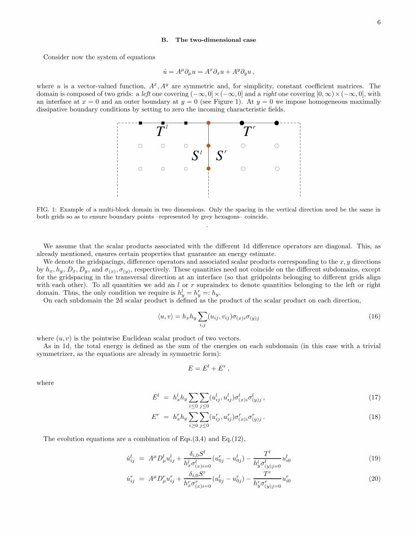
where u is a vector-valued function, Ax, Ay are symmetric and, for simplicity, constant coefficient matrices. Thedomain is composed of two grids: a left one covering (−∞, 0]× (−∞, 0] and a right one covering [0,∞)× (−∞, 0], withan interface at x = 0 and an outer boundary at y = 0 (see Figure 1). At y = 0 we impose homogeneous maximallydissipative boundary conditions by setting to zero the incoming characteristic fields.

FIG. 1: Example of a multi-block domain in two dimensions. Only the spacing in the vertical direction need be the same inboth grids so as to ensure boundary points –represented by grey hexagons– coincide.

.

We assume that the scalar products associated with the different 1d difference operators are diagonal. This, asalready mentioned, ensures certain properties that guarantee an energy estimate.We denote the gridspacings, difference operators and associated scalar products corresponding to the x, y directions

by hx, hy, Dx, Dy, and σ(x), σ(y), respectively. These quantities need not coincide on the different subdomains, exceptfor the gridspacing in the transversal direction at an interface (so that gridpoints belonging to different grids alignwith each other). To all quantities we add an l or r supraindex to denote quantities belonging to the left or rightdomain. Thus, the only condition we require is hl

y = hry =: hy.

On each subdomain the 2d scalar product is defined as the product of the scalar product on each direction,

〈u, v〉 = hxhy

∑

i,j

(uij , vij)σ(x)iσ(y)j (16)

where (u, v) is the pointwise Euclidean scalar product of two vectors.As in 1d, the total energy is defined as the sum of the energies on each subdomain (in this case with a trivial

symmetrizer, as the equations are already in symmetric form):

E = El + Er ,

where

El = hlxhy

∑

i≤0

∑

j≤0

(ulij , u

lij)σ

l(x)iσ

l(y)j , (17)

Er = hrxhy

∑

i≥0

∑

j≤0

(urij , u

rij)σ

r(x)iσ

r(y)j . (18)

The evolution equations are a combination of Eqs.(3,4) and Eq.(12),

ulij = AµDl

µulij +

δi,0Sl

hlxσ

l(x)i=0

(ur0j − ul

0j)−T l

hlyσ

l(y)j=0

uli0 (19)

urij = AµDr

µurij +

δi,0Sr

hrxσ

r(x)i=0

(ul0j − ur

0j)−T r

hryσ

r(y)j=0

uri0 (20)

7

In the above expressions, Sl, Sr, T l, T r are operators (as opposed to scalars), since we are dealing with a system ofequations. The first two correspond to penalty terms added to handle grid interfaces while the latter two for imposingouter boundary conditions. The goal of these operators is to transform to characteristic variables and apply to theevolution equation of each characteristic mode suitable penalty terms, as in Eqs.(3,4,12).Taking a time derivative of the energies defined in Eq.(17,18), using the evolution equations (19,20), and employing

the SBP property along each direction, one gets

El = hy

∑

j≤0

σl(y)j

[

(ul0,j , (A

x − 2Sl)ul0,j) + 2(ul

0,j, Slur

0,j)]

+ hlx

∑

i≤0

σl(x)i(u

li,0, (A

y − 2T l)uli,0) (21)

Er = hy

∑

j≤0

σr(y)j

[

(ur0,j , (−Ax − 2Sr)ur

0,j) + 2(ur0,j, S

rul0,j)

]

+ hrx

∑

i≥0

σr(x)i(u

ri,0, (A

y − 2T r)uri,0) (22)

where we have assumed that S and T are hermitian matrices.In order to control the interface terms in El + Er we can take

Sl =1

σl(y)j

[

(Λ+a + δ+a )P

a+ + δ−a P

a− + δ0P0

]

,

Sr =1

σr(y)j

[

(−Λ−a + δ−a )P

a− + δ+a P

a+ + δ0P0

]

;

where a sum over the index a is assumed, and {P a+, P

a−, P0} are projectors to the sub-spaces of eigenvectors of Ax

with eigenvalues {Λ+a ,Λ

−a ,Λ

0} respectively. With this choice El + Er becomes

El + Er = hy

∑

j≤0

[

(Λ−a − 2δ−a )||ua,l

− − ua,r− ||2 − (Λ+

a + 2δ+a )||ua,l+ − ua,r

+ ||2 − 2δ0||ul0 − ur

0||2]

(23)

+ hlx

∑

i≤0

σl(x)i(u

li,0, (A

y − 2P l)uli,0) + hr

x

∑

i≥0

σr(x)i(u

ri,0, (A

y − 2P r)uri,0) . (24)

Clearly, in order to obtain an estimate, the following conditions must be satisfied,

Λ−a − 2δ−a ≤ 0, Λ+

a + 2δ+a ≥ 0, δ0 ≥ 0 ;

which is analogous to the one-dimensional case, Eqs.(9,10,11). Similarly, the outer boundary terms in El + Er (i.e.the sums over i) can be controlled on each domain separately. We need

ur(Ay − 2T r)ur ≤ 0 ,

ul(Ay − 2T l)ul ≤ 0 .

We can therefore take, as in the one-dimensional case,

P r = P l = (Λ+a + δ+a )P

+a ,

where now P a+ are projectors to the spaces of eigenvectors of Ay of eigenvalues Λ+

a . With these choices the finalexpression for the time derivative of the energy is

El + Er = hy

∑

j≤0

[

(Λ−a − 2δ−a )||ua,l

− − ua,r− ||2 − (Λ+

a + 2δ+a )||ua,l+ − ua,r

+ ||2 − 2δ0||ul0 − ur

0||2]

(25)

+ hlx

∑

i≥0

σl(x)i(−Λ−

a − 2δ−a )||ua,l− ||2 + hr

x

∑

i≥0

σr(x)i(−Λ−

a − 2δ−a )||ua,r− ||2 (26)

and, again, the possible ranges for the different δ’s are as in the 1d case, Eqs.(9,10,11).Notice that nothing special has to be done at a corner, as each direction is treated and controlled independently.

8

C. The general case

The general case follows the same rules. Namely, we must add penalty terms on the characteristic modes corre-sponding to each of the boundary matrices separately and accordingly.For example, what to do at the vertices of three patches meeting in the cubed-sphere case discussed later in this

paper? As we will see, there we have three meshes with coordinates (at a constant radius) (a1, b1), (a2, b2), and(a3, b3) arranged in a clockwise distribution according to the indices, and intersecting at a point. In that case, thecontribution to the energy (without the penalty terms added to the evolution equations) is proportional to

(u10N , (Aa1

+Ab1)u10N ) + (u2

00, (Aa2

+Ab2)u200) + (u3

0N , (Aa3

+Ab3)u30N )

Since the interfaces are aligned to the grids we know that the normals coincide on both sides, therefore we have:

Aa1

= Aa3

Ab1 = Ab2 Ab3 = Aa2

So we include penalty terms on each side, including the end-points of the grids in each direction, (which constitutevertices and edges). Note that the characteristic modes at these points are computed with the normal with respectto the side that contains this direction. Consequently, points at edges/vertices of a (topologically) cubical grid willhave two/three penalty terms.

III. HIGH ORDER DIFFERENCE OPERATORS WITH DIAGONAL NORMS

In this section we analyze some aspects of Strand’s 1d difference operators satisfying SBP with respect to diagonalmetrics, when used in conjuction with the penalty technique to construct high order schemes for handling domainswith interfaces.In particular, we discuss operators with accuracy of order two, four, six and eight at interior points. The requirement

that these operators satisfy the SBP property with respect to diagonal norms implies that their respective accuracyorder at and close to boundaries is one, two, three and four, respectively. We will therefore refer to these operators asD2−1, D4−2, D6−3, and D8−4. Some of these operators are not unique, as the accuracy order and SBP requirementsstill leave in some cases additional freedom in their construction. Indeed, while the first two operators (D2−1, D4−2)are unique, the D6−3 one comprises a mono-parametric family, and D8−4 a three-parametric one. This freedom canbe exploited for several purposes. For instance, to minimize the operator’s bandwidth or its spectral radius. Whilethe former produces operators which are more compact, the latter can have a significant impact on the CFL limitwhen dealing with evolution equations. Indeed, for the D8−4 case, minimizing its bandwidth leads to a considerablylarger spectral radius (though this does not happen in the D6−3 case) which, in turns, requires one to employ a rathersmall CFL factor for the fully discrete scheme to be stable.To analyze this in each case, we numerically solve and discuss the eigenvalues of the amplification matrix of the

advection equation with speed one, ut = u′, under periodic boundary conditions. The periodicity is imposed throughan interface with penalty terms and hence the scheme does depend on the penalty parameter δ and so will the discreteeigenvalues obtained. As discussed in Section II, in the case in which δ = −1/2, SBP holds across the interface,and the energy for this model is strictly conserved. In other words, the amplification matrix is anti-symmetric andthe eigenvalues are purely imaginary (see Section II). On the other hand, if δ > −1/2 there is a negative definiteinterface term left after SBP, and a negative real component in the eigenvalues must appear in the spectrum of theamplification matrix (see Section II).We additionally discuss the global convergence factor for these operators, and recall a feature associated with the

mode with highest possible group speed at a given number of gridpoints. Namely, that it travels in the “wrong”direction, and that the absolute value of its speed increases considerably with the order of the operator.Appendix A lists, for completeness, some typos in Ref. [9] in some of the coefficients for these high order operators.

A. Spectrum

In the following we discuss the range of discrete eigenvalues obtained for the different derivative operators and theirdependence on δ. We pay particular attention on the impact different values of δ and the chosen derivative operatorhave on the CFL limit.

9

1. Second order in the interior, first order at boundaries (D2−1 scheme)

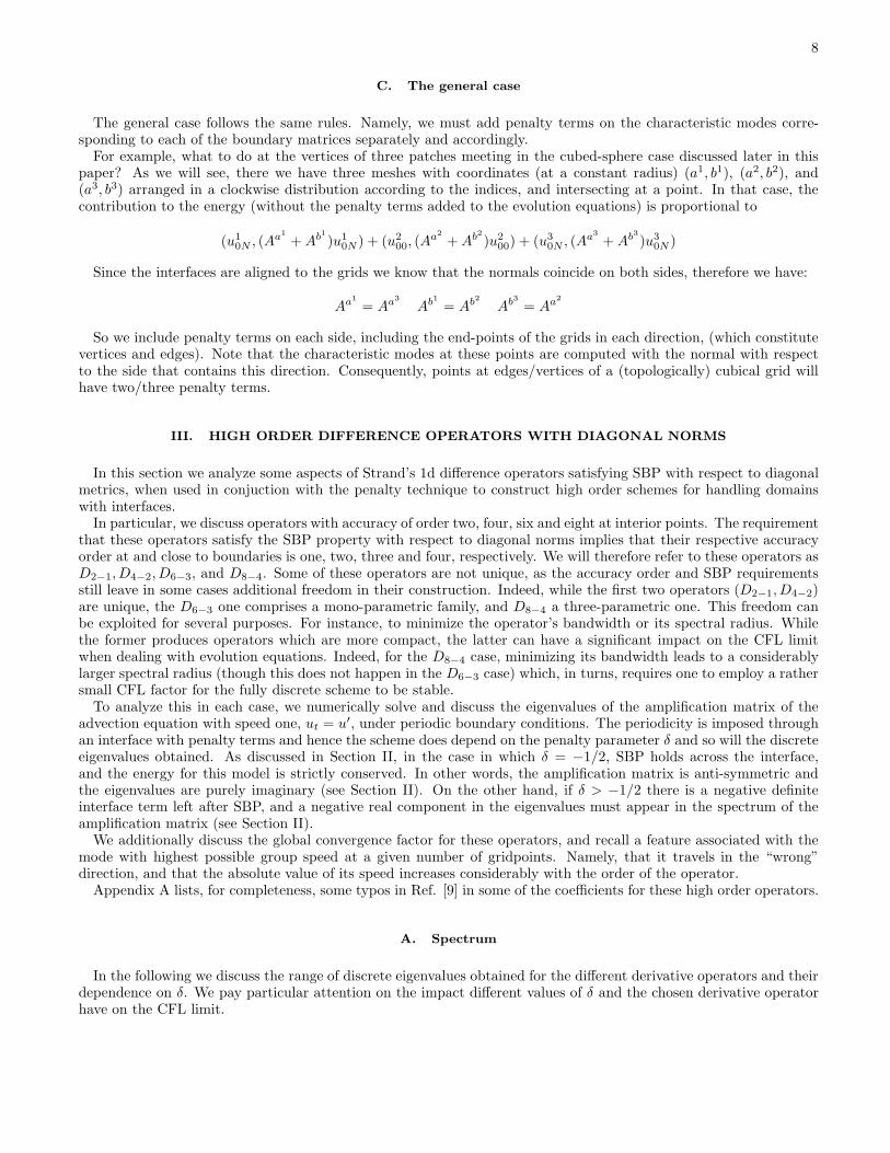
Figure 2 shows the eigenvalues obtained using 20, 60, 100 gridpoints and penalty term δ = −1/2 (that is, the purelyimaginary spectrum case, see Section II) for the D2−1 case. The maximum and minimum values are, approximately,±1.414, and they seem to be related to the operator near the boundary, as their absolute value does not seem toincrease with the number of points (instead, the region between the maximum and minimum is filled out). As discussedbelow, in the higher order cases the maximum eigenvalues also seem to be related to the operator near the boundary.

–1

–0.5

0

0.5

1

–1e–10 –5e–11 0 5e–11 1e–10

–1

–0.5

0

0.5

1

–1e–10 –5e–11 0 5e–11 1e–10

–1

–0.5

0

0.5

1

–1e–10 –5e–11 0 5e–11 1e–10

FIG. 2: Numerically obtained eigenvalues (in the complex plane) corresponding to the D2−1 operator for δ = −1/2 (purelyimaginary case). From left to right the plots illustrate the results obtained with a grid containing 20, 60, 100 points respectively.It is clear from the figures that these correspond, indeed, to a purely imaginary case.

Figure 3, in turn, shows the eigenvalues computed with 100 points and δ = 0, 1/10, 1/2. A negative real partappears, as it should (based on the energy calculation), and the maximum in the imaginary axis slightly decreases(to approximately 0.999, not varying much among these three values). However, the maximum absolute value in thenegative real axis grows quite fast with δ. For example, for δ = 1/10 such maximum already dominates over themaximum in the imaginary axis. The higher order operators analyzed below behave similarly.

2. Fourth order in the interior, second order at and close to boundaries (D4−2 scheme)

Figure 4 shows the equivalent of Figure 2, but now for the D4−2 case. The maximum is slightly larger than thecorresponding one for the D2−1 case: approximately 1.936.Figure 5, in turn, shows the equivalent of Figure 3 for the current case. As before, a negative real part appears and

the maximum in the imaginary axis slightly decreases (in this case to roughly 1.371, not changing much among thesethree values of δ).

3. Sixth order in the interior, third order at and close to boundaries, minimum bandwidth case (D6−3 scheme)

Figure 6 illustrates the equivalent of Figures (2,4) for the D6−3 case. The maximum is roughly 2.129, slightly largerthan those of the previous two cases. The behavior for larger values of δ is similar to that one found in the previoustwo cases, as seen in Figure 7. The maximum in the imaginary axis again decreases slightly compared to the δ = −1/2case (to roughly 1.585) and does not change much among these three values of δ.

10

–1

–0.5

0

0.5

1

–1 –0.5 0 0.5 1

–1

–0.5

0

0.5

1

–4 –2 0 2 4

–1

–0.5

0

0.5

1

–4 –2 0 2 4

FIG. 3: Eigenvalues corresponding to the D2−1 operator, obtained with a grid containing 100 points. From left to right theplots illustrate the behavior for δ = 0, 1/10, 1/2 respectively. As δ becomes larger, a larger (in magnitude) negative eigenvalueon the real axis is observed (notice the left-most diamond at y ≃ −1.6,−3.5 on the middle and right plots, respectively).

–2

–1

0

1

2

–1e–10 –5e–11 0 5e–11 1e–10

–2

–1

0

1

2

–1e–10 –5e–11 0 5e–11 1e–10

–2

–1

0

1

2

–1e–10 –5e–11 0 5e–11 1e–10

FIG. 4: Numerically obtained eigenvalues corresponding to the D4−2 operator for δ = −1/2 (purely imaginary case). Fromleft to right the plots illustrate the results obtained with a grid containing 20, 60, 100 points respectively. It is clear from thefigures that these correspond, as in Fig.2, to a purely imaginary case.

4. Eight order in the interior, fourth order at and close to boundaries (D8−4 scheme)

The D8−4 operator has three free parameters, denoted as x1, x2, x3 both in Ref.[9] and here. As mentioned, theseparameters can be freely chosen to satisfy a given criteria. For instance, they can be fixed so as to minimize the widthof the derivative operator or yield as small a spectral radius as possible. As we discuss next, these options can yieldoperators with significantly different stability requirements as dictated by the CFL condition.Minimum bandwidth operator. The minimum bandwidth case corresponds to the choice (see [9])

x1 =1714837

4354560, x2 = − 1022551

30481920, x3 =

6445687

8709120. (27)

Figure 6 shows for this minimum D8−4 bandwidth case the eigenvalues for 20, 60, 100 points, for δ = −1/2 (purely

11

–1

–0.5

0

0.5

1

–1 –0.5 0 0.5 1

–1

–0.5

0

0.5

1

–4 –2 0 2 4

–1

–0.5

0

0.5

1

–4 –2 0 2 4

FIG. 5: Eigenvalues corresponding to the D4−2 operator, obtained with a grid containing 100 points. From left to right theplots illustrate the behavior for δ = 0, 1/10, 1/2 respectively. As δ becomes larger, a larger (in magnitude) negative eigenvalueon the real axis is observed (notice the left-most diamond at y ≃ −2.5,−5 on the middle and right plots, respectively).

–2

–1

0

1

2

–1e–10 –5e–11 0 5e–11 1e–10

–2

–1

0

1

2

–1e–10 –5e–11 0 5e–11 1e–10

–2

–1

0

1

2

–1e–10 –5e–11 0 5e–11 1e–10

FIG. 6: Numerically obtained eigenvalues corresponding to the minimum bandwidth D6−3 operator for δ = −1/2 (purelyimaginary case). From left to right the plots illustrate the results obtained with a grid containing 20, 60, 100 points respectively.As in Figs.(2,4), these correspond to a purely imaginary case.

imaginary case). While for the previous operators we have seen that the maximum eigenvalue increases slightly withthe order of the operator, in this case the increase is quite large: the maximum is roughly 16.04. This translates intoa CFL limit for this operator being almost an order of magnitude smaller than the limits for the previous operators.Additionally, variation of δ does not significantly affect this behavior, as shown in Figure 9. That figure shows theeigenvalues computed with 100 points, and δ = 0, 1/10, 1/2. The qualitative behavior when increasing δ is similar tothat one of the previous cases. A negative real part appears in the spectrum, and the maximum in the imaginaryaxis slightly decreases, to roughly 16.02, not varying much among these three illustrative values of δ. Such a largespectral radius for this operator motivates the search for another one, with a more convenient radius at the expenseof not having the minimum possible bandwidth.Optimized operator. We here construct an “optimized D8−4 operator” (which we shall use from here on in the

D8−4 case) in the sense that it has a spectral radius considerably smaller than that one defined by Eq.(27). More

12

–1.5

–1

–0.5

0

0.5

1

1.5

–1 –0.5 0 0.5 1

–1.5

–1

–0.5

0

0.5

1

1.5

–6 –4 –2 0 2 4 6

–1.5

–1

–0.5

0

0.5

1

1.5

–6 –4 –2 0 2 4 6

FIG. 7: Eigenvalues corresponding to the D6−3 operator obtained with a grid containing 100 points. From left to right theplots illustrate the behavior for δ = 0, 1/10, 1/2 respectively. As δ becomes larger, a larger (in magnitude) negative eigenvalueon the real axis is observed (notice the left-most diamond at y ≃ −2.5,−6 on the middle and right plots, respectively).

–15

–10

–5

0

5

10

15

–1e–10 –5e–11 0 5e–11 1e–10

–15

–10

–5

0

5

10

15

–1e–10 –5e–11 0 5e–11 1e–10

–15

–10

–5

0

5

10

15

–1e–10 –5e–11 0 5e–11 1e–10

FIG. 8: Numerically obtained eigenvalues corresponding to the minimum bandwidth D8−4 operator for δ = −1/2 (purelyimaginary case). From left to right the plots illustrate the results obtained with a grid containing 20, 60, 100 points, respectively.Although purely imaginary, the maximum (absolute) value in the vertical axis is approximately 16.

precisely, through a numerical search in the three-parameter space we have found that the following values

x1 = 0.541, x2 = −0.0675, x3 = 0.748 , (28)

yield an operator whose maximum absolute eigenvalue in the purely imaginary case (δ = −1/2) is

λmax = 2.242 . (29)

This maximum eigenvalue appears to be quite sensitive on these parameters. For example, truncating the abovevalues to two significant digits,

x1 = 0.54, x2 = −0.067, x3 = 0.75 ,

13

–15

–10

–5

0

5

10

15

–1 –0.5 0 0.5 1

–15

–10

–5

0

5

10

15

–8 –6 –4 –2 0 2 4 6 8

–15

–10

–5

0

5

10

15

–8 –6 –4 –2 0 2 4 6 8

FIG. 9: Eigenvalues for the minimum bandwidth D8−4 operator with δ = 0, 1/10, 1/2 (from left to right) and 100 points. Valuesof δ larger than −1/2 introduce a negative real part in the spectrum but they have little effect on the maximum absolute value,which remains at approximately 16.

gives λmax = 2.698 and truncating even more, to just one digit,

x1 = 0.5, x2 = −0.07, x3 = 0.7 ,

gives the large value λmax = 71.76. On the other hand, refining in the parameter search the values in Eq.(28) in onemore digit did not change the maximum of Eq.(29) in its four digits here shown. The eigenvalues for δ = −1/2 forthis optimized D8−4 operator, given by the parameters of Eq.(28), are shown in Figure 10, while Figure 11 shows

–2

–1

0

1

2

–1e–10 –5e–11 0 5e–11 1e–10

x

–2

–1

0

1

2

–1e–10 –5e–11 0 5e–11 1e–10

x

–2

–1

0

1

2

–1e–10 –5e–11 0 5e–11 1e–10

x

FIG. 10: Eigenvalues for the optimized D8−4 operator with δ = −1/2 (purely imaginary case), and 20, 60, 100 points (from leftto right). Clearly, this modified operator has a much smaller spectral radius, compared to the minimum bandwidth one.

them for δ = 0, 1/10, 1/2 and 100 points. As before, a negative real component appears and the maximum in theimaginary axis decreases (to around 1.754).While completing this work we became aware of similar work by Svard, Mattson and Nordstrom [14], who construct

an optimized operator with different parameters by minimizing the spectral radius of the derivative itself (rather thanthat of the amplification matrix of a toy problem with an interface, as in our case), obtaining x1 = 0.649, x2 =

14

–1.5

–1

–0.5

0

0.5

1

1.5

–1 –0.5 0 0.5 1

–1.5

–1

–0.5

0

0.5

1

1.5

–6 –4 –2 0 2 4 6

–1.5

–1

–0.5

0

0.5

1

1.5

–6 –4 –2 0 2 4 6

FIG. 11: Eigenvalues for the optimized D8−4 operator, with 100 points and δ = 0, 1/10, 1/2 (from left to right).

−0.104, x3 = 0.755. When using these parameters in our toy problem with an interface, the resulting spectral radius(for twenty gridpoints) is λmax = 2.241259, while for the parameters we chose [cf. Eq.(28)] is λmax = 2.241612 [15].

B. Global convergence rate

In general, the global (say, in an L2 norm) convergence factor for these operators will be dominated by the lowerorder at and close to boundaries. However, it is sometimes found that roundoff values for the error in such a globalnorm are reached before this happens, and the convergence factor is different from the one expected from the boundaryterms. The precise value is found to actually depend on the function being differentiated and whether one reachesround-off level. To illustrate the expected behavior in a generic case, we consider the function sin(10x) + cos(10x) inthe domain x ∈ [0, 2π]. Figure 12 shows the error (with respect to the exact solution) when computing the discretederivative versus the number of gridpoints, for the difference operators D2−1, D4−2, D6−3, and D8−4. The errors inthe L2 norm are shown until roundoff values are reached (further increasing the number of gridpoints causes the errorto grow with the number of points involved). Figure 13, in turn, shows the obtained convergence factors.

C. Group Speed

We now turn our attention to the group speed that different discrete modes have when the above consideredoperators are used. To simplify the discussion, we actually restrict ourselves to the periodic case, which lends itselffor a clean analytical calculation. In this case the operators of order two, four, six and eight satisfying SBP are thestandard, centered ones (D0, D+, D− denote the standard centered second order, and forward and backward firstorder operators, respectively):

D(2) = D0 (30)

D(4) = D0(I − h2/6D+D−) (31)

D(6) = D0(I − h2/6D+D− + h4/30D2+D

2−) (32)

D(8) = D0(I − h2/6D+D− + h4/30D2+D

2− − h6/140D3

+D3−) (33)

(34)

In discrete Fourier space, the eigenvalues for these operators are, respectively,

λ2 = sin(ζ)/ζ , (35)

λ4 = sin(ζ)/ζ(1 + 2 sin(ζ/2)/3) , (36)

15

2 3 4 5 6 7log10(Npts)

-20

-15

-10

-5

0

Err

ors

D2-1

D4-2

D6-3

D8-4

Errors with respect to u=sin(10 x) + cos(10 x)

FIG. 12: L2 norms of the errors obtained when taking the discrete derivative of sin(10x) + cos(10x) and comparing it with theanalytical answer, using D2−1, D4−2, D6−3, D8−4 operators, versus the number of gridpoints.

2 3 4 5 6 7log10(Npts)

0

1

2

3

4

5

Con

verg

ence

fact

or

D2-1D4-2D6-3D8-4

Convergence factor with respect to u=sin(10 x) + cos(10 x)

FIG. 13: Convergence factors for the curves of Figure 12. As in this case, the convergence in general will be dictated by thelower order the derivative operators have at and close to the boundaries. Note that the lines corresponding to the differentoperators terminate at sequentially fewer points. This is due to the corresponding errors reaching round-off levels, after whichthe convergence factor calculation ceases to have a sensible meaning.

λ6 = sin(ζ)/ζ(1 + 2 sin(ζ/2)/3 + 8 sin4(ζ/2)/15) , (37)

λ8 = sin(ζ)/ζ(1 + 2 sin(ζ/2)/3 + 8 sin4(ζ/2)/15 + 64 sin6(ζ/2)/140) . (38)

where ζ = ωh, and ω is the associated wave number.The highest possible frequency is ω = N/2 (with N the number of gridpoints). For that frequency, ζ = π and the

above eigenvalues are all zero. Therefore the mode with highest possible frequency for a given number of points does

16

not propagate. Furthermore, if one examines the group speed,

vg =d(λω)

dω, (39)

one finds that at ζ = π this speed is

v2g = −1 , (40)

v4g = −5/3 ≈ −1.6 , (41)

v6g = −33/15 ≈ −2.2 , (42)

v8g = −341/135 ≈ −2.6 . (43)

Thus, for higher (than two) order operators the velocity of this mode is higher than the continuum one (which is 1).But, more importantly, in all cases the speed has the opposite sign. Of course, this effect goes away with resolution,since the highest possible frequency moves to larger values as resolution is increased. But, still, is an effect to be takeninto account. For instance, if noise is produced at an interface, it propagates backwards, and with higher speed. Eventhough this effect is typically very small, it might be noticeable in highly accurate simulations, or in simulations inwhich the solution itself decays to very small values (see Section IVC2). This could also be a source of difficultiesin the presence of black holes –or for this matter any system where some propagation speed changes sign– since theevent horizon traps these high frequency modes in a very narrow region and then releases them as low frequency ones.We have observed this in some highly resolved one dimensional simulations, and explains an observed convergencedrop which goes away when numerical dissipation is turned on.

IV. TESTS

In this section we illustrate the behavior of the aforementioned penalty technique, together with the choice ofdifferent derivative operators. We present tests in one, two and three dimensions. In particular, we implementthe linearized Einstein equations (off a ‘gauge-wave’ spacetime [16, 17]) and propagation of scalar fields in blackhole backgrounds. The former is cast in a way which yields a one-dimensional symmetric hyperbolic system withcoefficients depending both in space and time while the latter provides an hyperbolic system of equations with spacevarying coefficients and sets a conforming grid for spherical black hole excision.Throughout this paper we employ a fourth order accurate Runge–Kutta time integrator. In a number of tests aimed

at examining the behavior of high order operators we adopt a sufficiently small time step ∆t so that the time integratordoes not play a role. Thus, we either choose a suitably small CFL factor or we scale the time step quadratically withthe gridspacing h.

A. One dimensional simulations: linearizations around a gauge wave

As a first test we evolve Einstein’s equations in one dimension, linearized around a background given by

ds2 = eA sin(π(x−t))(−dt2 + dx2) + dy2 + dz2. (44)

This background describes flat spacetime with a sinusoidal coordinate dependence, of amplitude A, along the xdirection. One of the interesting features of this testbed is that while a linear problem, the coefficients in theequations to solve are not only space but also time dependent.The non-trivial variables for this metric are

gxx = eA sin(π(x−t)) , (45)

Kxx =A

2π cos (π (x− t)) eA/2 sin(π(x−t)) , (46)

α = eA/2 sin(π(x−t)) , (47)

βi = 0 . (48)

We evolve the linearized Einstein equations using the symmetric hyperbolic formulation presented in Ref. [18] with adynamical lapse given by the homogeneous time-harmonic condition (defined by requiring �t = 0). The formulation is

17

cast in first order form by introducing the variables Ax := ∂xα/α and dxxx := ∂xgxx. The equations determining thedynamics of the (first order) perturbations, which we assume to depend solely on (t, x), are obtained by consideringlinear deviations of a background metric given by Eq. (44). That is, we consider

gxx = gxx + δgxx,

Kxx = Kxx + δKxx,

dxxx = dxxx + δdxxx,

α = α+ δα,

Ax = Ax + δAx ;

replace these expressions in Einstein’s equations and retain only first order terms. The resulting equations are(henceforth dropping the δ notation)

α = −Aπ cos(φ)α−Kxx +Aπ

2αcos(φ)gxx , (49)

Ax = − 1

α∂xKxx +

Aπ

2αcos(φ)Kxx ,

−Aπ2

2α2

(

A cos(φ)2 + sin(φ))

gxx

+Aπ

2α2cos(φ)dxxx

−Aπ

2cos(φ)Ax +

Aπ2

2αsin(φ)α , (50)

gxx = −Aαπ cos(φ)α − 2αKxx , (51)

Kxx = −α∂xAx − Aαπ

2cos(φ)Ax

−Aπ2

4

(

−2 sin(φ) +A cos(φ)2)

α

−Aπ cos(φ)Kxx

+Aπ

4αcos(φ)dxxx , (52)

dxxx = Aαπ2(

sin(φ) −A cos(φ)2)

α

−Aαπ cos(φ)Kxx −Aα2π cos(φ)Ax

−2α∂xKxx , (53)

where we have defined φ := π(x − t). This system is symmetric hyperbolic and the symmetrizer used to define theenergy can be chosen so that the characteristic speeds which play a role in the energy estimate are 0 and ±1.We consider here a periodic initial boundary value problem on the domain x ∈ [−1/2, 3/2], where periodic boundary

conditions at x = −1/2, 3/2 are implemented through an interface with penalty terms, as described in Section II.The system must satisfy two non-trivial constraint equations, corresponding to the definition of the variables dxxx

and Ax (the linearized physical constraints are automatically satisfied by the considered ansatz). When linearized,these constraints are

0 = Cx = −∂xgxx + dxxx , (54)

0 = CA = Ax − 1

α

(

∂xα− Aπ

2cos(φ)α

)

. (55)

In the first series of simulations we adopt a CFL factor λ = 10−3[39] and consider relatively short evolutionscorresponding to four crossing times. The D8−4 derivative is used, and dissipation is added through the dissipativeoperator constructed from −σh7D4

+D4−, suitably modified at boundaries as explained in Appendix B so as to make

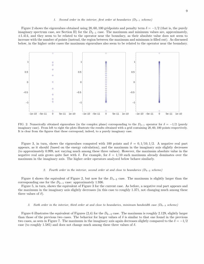
it non-positive definite with respect to the appropriate scalar product. Thus, the use of this dissipative operator doesdecrease the order of the spatial discretization by one. The dissipation parameter used is σ = 5 × 10−4. Figure 14exemplifies the behavior observed in the convergence of the field Kxx (the other fields behave similarly). As timeprogresses the convergence order obtained oscillates in a way that is consistent with the accuracy obtained at interiorand boundary points.

18

0 2 4 6 8time

0

2

4

6

8

Con

verg

ence

fact

or

41-81-16181-161-321321-641-1281

FIG. 14: Evolutions of 1d linearized Einstein’s equations in a periodic domain, with periodicity enforced through an interfacewith penalty terms. Shown is the convergence factor for Kxx when using the D8−4 derivative, CFL factor λ = 10−3, anddissipation σ = 5 × 10−4. While the convergence factors obtained with 41 to 321 points oscillate between the expected orderat the boundary and that one at the interior, the ones calculated with 321 to 1281 points are not meaningful when the pulseis located at interior points as round-off level is reached.

Next, we adopt as a starting value for the CFL factor defined at the coarsest grip to be λ = 0.2 but in subsequentgrids (refined by a factor of 2) we adopt λ = 0.2/2n with (n = 1..3). Figure 15 illustrates the behavior observed;again, as time progresses the convergence order obtained oscillates in between the order of accuracy of interior andboundary points, with the additional effect of accuracy loss due to the accumulation of error as time progresses.

0 20 40 60 80 100time

4

4.5

5

5.5

6

6.5

7

Con

verg

ence

fact

or

41-81-16181-161-321

FIG. 15: Same as previous figure, but with a decreasing CFL factor given by λ = 0.2/2n with (n = 1..3).

.

Finally, we compare the above results with those obtained in the “truly periodic case”, ie. when periodicity is usedexplicitly to employ the same derivative operator at all points. We again consider cases where a sufficiently smallCFL factor (= 10−3) is used or the time-step is scaled quadratically. Figures 16 illustrates the observed convergencerate for the field gxx. As above, dissipation is added through a seventh order dissipative operator (but now withno modification at boundaries needed) with same dissipative parameter: σ = 5 × 10−4. While the errors remainabove round-off level the observed convergence rate is consistent with the expected one of seven, as the orders of the

19

derivative and dissipative operators employed are eight and seven respectively. Certainly, dissipation of higher ordercould have been introduced by simply employing the KO style operator h9(D−D+)

5, but we have adopted this one tomore directly compare with the case with interface boundaries. For the highest resolutions the errors reach round-offlevel and the obtained convergence factors yield non-sensible values.

0 2 4 6 8time

0

2

4

6

8

Con

verg

ence

fact

or

40-80-16080-160-320160-320-640320-640-1280640-1280-25601280-2560-5120

Convergence factor (D8)Gauge wave, periodic boundary conditions, λ=0.001

0 20 40 60 80 100time

2

3

4

5

6

7

Con

verg

ence

fact

or

21-41-8141-81-16181-161-321

Convergence factors (D8)Gauge wave, periodic boundary conditions, quadratic λ

FIG. 16: This figure shows evolutions similar to those of Figs.14, 15, with the only difference that periodicity is here enforcedexplicitly. The convergence factors for the metric component gxx are shown.

.

As an illustration of what is observed with other derivatives, we briefly discuss some simulations using the D6−3

operator and a fixed CFL factor (given, as before, by λ = 10−3). Analogously as to was done above, dissipation ishere added by extending –as discussed in Appendix B– the operator σh6D3

−D3+ at and near boundaries in order to

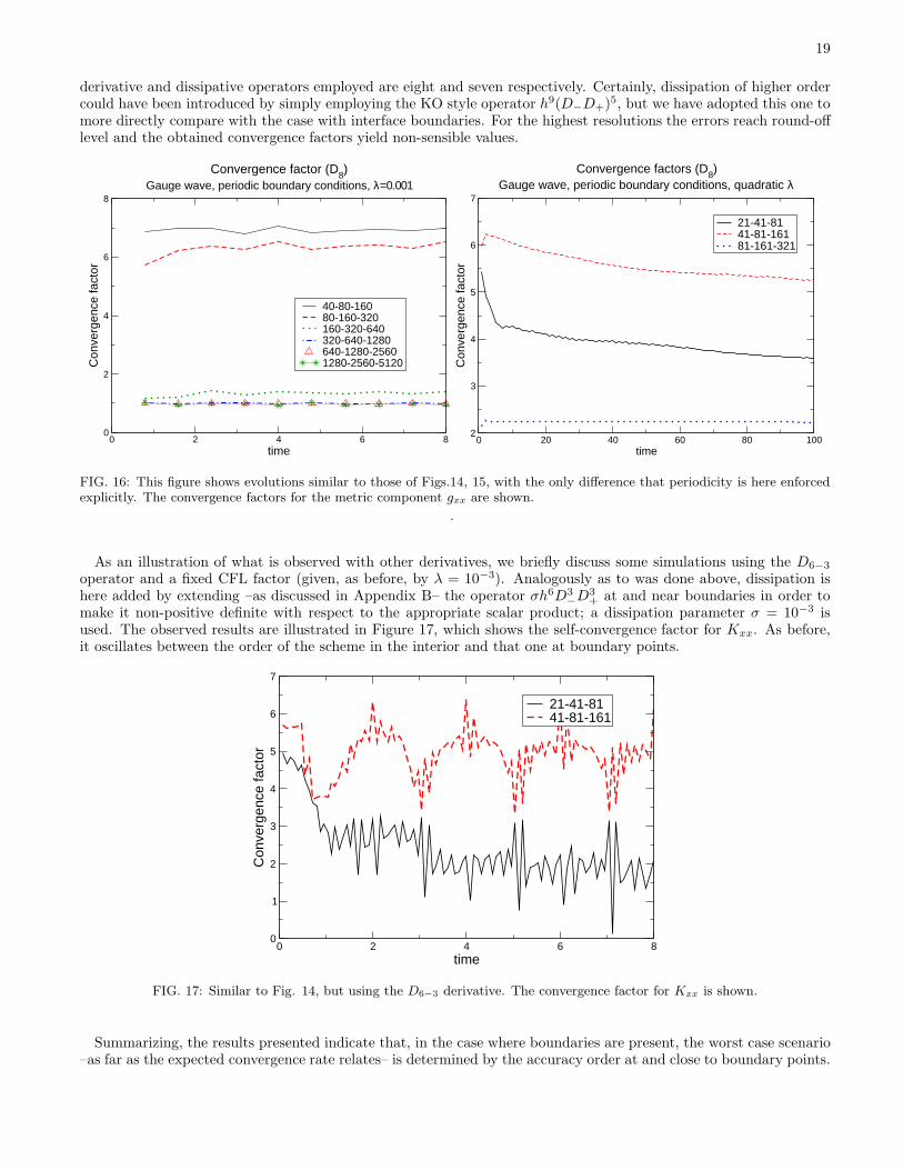
make it non-positive definite with respect to the appropriate scalar product; a dissipation parameter σ = 10−3 isused. The observed results are illustrated in Figure 17, which shows the self-convergence factor for Kxx. As before,it oscillates between the order of the scheme in the interior and that one at boundary points.

0 2 4 6 8time

0

1

2

3

4

5

6

7

Con

verg

ence

fact

or

21-41-8141-81-161

FIG. 17: Similar to Fig. 14, but using the D6−3 derivative. The convergence factor for Kxx is shown.

Summarizing, the results presented indicate that, in the case where boundaries are present, the worst case scenario–as far as the expected convergence rate relates– is determined by the accuracy order at and close to boundary points.

20

Two and three-dimensional simulations. Problem set-up

In this section we solve the wave equation for a scalar field φ propagating on a fixed background,

∇a∇aφ = 0 ,

where ∇ is the covariant derivative associated with the metric of the background. We will consider two backgrounds:a 2d one consisting of the unit sphere with its standard metric and a 3d one consisting of a rotating Kerr black holebackground.We start by describing in more detail the equations solved and the multiple coordinate system used, and then

present the actual results of the simulations.

A strictly stable scheme for the wave equation in a time-independent, curved spacetime

The wave equation in a time-independent background can be written, using any coordinates in which the metric ismanifestly time independent as,

φ = αΠ (56)

Π = βiα−1Di(αΠ) + h−1/2Di(h1/2βiΠ+ αh1/2Hijdj) (57)

di = Di(απ) (58)

where Hij := hij −α−2βiβj , hij is the inverse of the three-metric, h = det(hij), α is the lapse and βi the shift vector.The advantage of writing the equations in this way is that one can show that if D is any difference operator satisfyingSBP, this form of the equations guarantees that the semidiscrete version of the physical energy is a non-increasingfunction of time. When the killing field is timelike this means that there is a norm in which the solution is bounded forall times, thus suppressing artificial fast growing-modes without the need of artificial dissipation (see [19] for details).We now look at the characteristic variables and characteristic speeds with respect to a “coordinate” observer. That

is, the eigenfields and eigenvalues of the symbol Aini, where Ai denotes the principal part of the evolution equationsand ni the normal to the boundary [40]. The characteristic variables with non-zero speeds

λ± = (±α+ βknk)(hijninj)

1/2

[where nk = nk(hijninj)

−1/2] are

v± = λ±Π+ αHij nidj ;

while the zero speed modes are

v0i = di − nidj nj .

Cubed-sphere coordinates.

The topology of the computational domain in our 2d simulations is S2, the unit sphere, while in our 3d ones it isS2 ×R+. Since it is not possible to cover the sphere with a single system of coordinates which is regular everywhere,we employ multiple patches to cover it. A convenient set of patches is defined by the cubed sphere coordinates, definedas follows (for a related definition see for instance [20]).

Each patch uses coordinates a, b, c, where c =√

x2 + y2 + z2, the standard radial coordinate, is the same for thesix patches (x, y, z are standard Cartesian coordinates). The other two coordinates, a, b are defined as

• Patch 0 (neighborhood of x = 1): a = z/x, b = y/x

• Patch 1 (neighborhood of y = 1): a = z/y, b = −x/y

• Patch 2 (neighborhood of x = −1): a = −z/x, b = y/x

• Patch 3 (neighborhood of y = −1): a = −z/y, b = −x/y

• Patch 4 (neighborhood of z = 1): a = −x/z, b = y/z

21

• Patch 5 (neighborhood of z = −1): a = −x/z, b = −y/z

Similarly, the inverse transformation is:

• Patch 0: x = c/D, y = cb/D, z = ac/D.

• Patch 1: x = −bc/D, y = c/D, z = ac/D

• Patch 2: x = −c/D, y = −cb/D, z = ac/D.

• Patch 3: x = bc/D, y = −c/D, z = ac/D

• Patch 4: x = −ac/D, y = cb/D, z = c/D

• Patch 5: x = ac/D, y = cb/D, z = −c/D

with D :=√1 + a2 + b2. This provides a relatively simple multi-block structure for S2 which can be exploited to

implement the penalty technique in a straightforward manner. Each patch is discretized with a uniform grid in thecoordinates a and b, and the requirement of boundary points coinciding in neighboring grids is indeed satisfied. Figure18 shows this gridstructure, for 20× 20 points on each patch.

–1

0

1

x

–1 –0.5 0 0.5 1

y

–0.5

0

0.5

1

z

FIG. 18: Cubed-sphere coordinates for S2.

.

B. 2d Simulations

We now discuss simulations of the wave equation on the unit sphere in cubed-sphere coordinates, written in strictlystable first order form [Eqs.(56,57,58)]. The metric used, therefore, is flat spacetime projected to the r = 1 slice,which in local coordinates is

ds2 = −dt2 +D−4[

(1 + b2) da2 + (1 + a2) db2 − 2 a b da db]

,

where D :=√

(1 + a2 + b2).Figure 19 shows simulations using the D4−2 derivative and its associated dissipative operator constructed in Ap-

pendix B, which we call KO6, using n × n points on each of the six patches, where n = 41, 81, 161, 321. The initialdata for Π corresponds to a pure l = 2,m = 1 spherical harmonic. The CFL factor used is λ = 0.125 and for each setof runs two values of dissipation are used: σ = 10−2 and σ = 10−3. As can be seen from the Figure, the self conver-gence factor obtained with these resolutions is above the lower value (two) expected from the order at the interfaces.The reason for the lower order at the interfaces not dominating is likely due to the fact that the initial data is aneigenmode of the Laplacian operator, and the solution at the continuum is just an oscillation in time of this initial

22

data, without propagation across the interfaces. Indeed, the oscillations in the convergence factors in Fig.19 appearwhen the numerical solution goes through zero, and the frequency at which this happens coincides approximatelywith the expected frequency at the continuum for this mode.The same initial data is now evolved with the D6−3 derivative and KO8 dissipation (again, see Appendix B) and

the results are shown in Figure 20. As before, λ = 0.125 and n = 41, 81, 161, 321 points are used, but the values ofdissipation shown are now σ = 0 (i.e., no dissipation) and σ = 10−3. At the same resolutions there is a small differencein the obtained convergence factors, depending on the value of σ, but with both values of this parameter the orderof convergence is higher than the lower one expected from the time integrator if this one dominated. Figure 20 alsopresents a comparison made with a smaller CFL factor: λ = 0.0125, keeping the dissipation at σ = 10−3. One moreresolution is used (641 points) to look for differences between the solutions obtained with the two CFL factors, butthey do not appear. This seems to suggest that at least in this case, and for these resolutions, it is not necessary touse too small a CFL factor in order to avoid the time integrator’s lowest order to dominate over the higher spatialdiscretization (see Fig.23 for another instance where this happens). It is also worth pointing out that the differencebetween the two highest resolutions is not quite at roundoff level, but it is rather small (of the order of 10−9 if scaledby the amplitude of the initial data), as shown in Figure 21. That figure shows the L2 norm of the differences betweenthe solution at different resolutions, for the simulations of Fig. 20 with λ = 0.0125 and σ = 10−3.

0 1 2 3 4time

2

2.5

3

3.5

4

4.5

541-81-161, σ=10

-3, λ=0.125

81-161-321, σ=10-3

, λ =0.125

41-81-161, σ=10-2

, λ=0.125

81-161-321, σ=10-2

, λ=0.125

2D Convergence Factor D4-2/KO6 l=2,m=1 initial data

FIG. 19: Evolutions of the wave equation on the unit sphere, using cubed-sphere coordinates and a pure l = 2,m = 1 sphericalharmonic as initial data. Shown is the convergence factor when the D4−2 derivative and the KO6 dissipation operators areused.

.

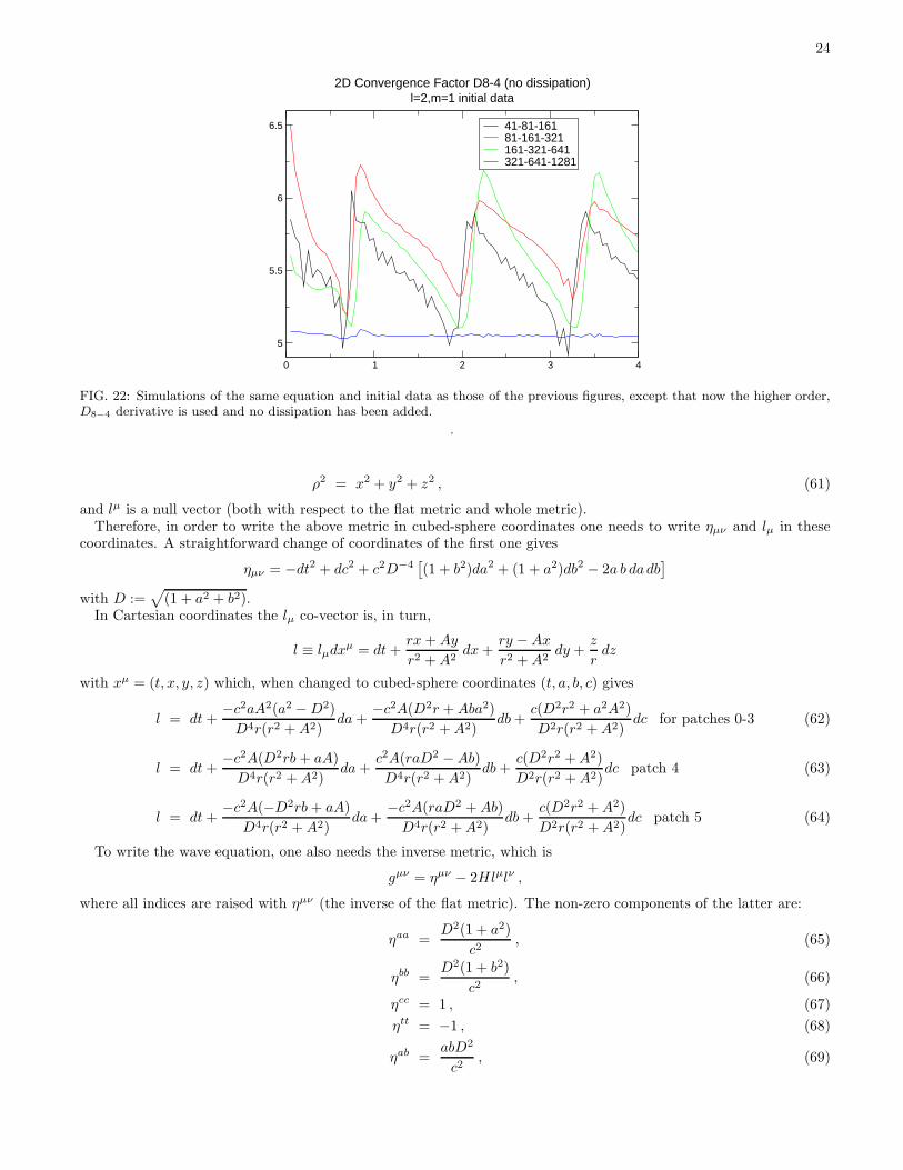
Finally, Figure 22 shows evolutions of the same initial data, with the D8−4 derivative, and no dissipation. The CFLfactor is decreased when resolution is increased, much as in Section IVA, so that the order of the time integrationdoes not dominate over the higher one of the spatial discretization. That is, for the resolutions shown we usedλ = 0.25, 0.125, 0.0625, 0.03125, 0.015625. The convergence factor obtained is also higher than that one expected fromthe lower order at the interfaces (presumably for the same reason as before, the initial data adopted) and higher thanthat one of the time integration.

C. Three dimensional simulations

In this application we consider fields propagating on a Kerr black hole background, as governed by equations(56,57,58), with the background metric written in Kerr-Schild form and cubed-sphere coordinates used for the an-gular directions. Homogeneous maximally dissipative boundary conditions are used at the outer boundary, whileno condition is needed at the inner one if it is appropriately placed inside the black hole so that it constitutes apurely-outflow surface.

23

0 1 2 3 4time

2

3

4

5

6

7

8

9

10

11

12

41-81-161, σ=10-3

81-161-321, σ=10-3

41-81-161, σ=081-161-321, σ=0

2D Convergence Factor D6-3/KO8 l=2,m=1 initial data, cfl=0.125

0 1 2 3 4time

2

3

4

5

6

7

8

9

10

11

12

41-81-161, λ=0.12581-161-321, λ=0.125161-321-641, λ=0.12541-81-161, λ=0.012581-161-321, λ=0.0125161-321-641, λ=0.0125

2D Convergence Factor D6-3/KO8 l=2,m=1 initial data, σ=10

-3

FIG. 20: Same evolution equation and initial data as those used in Figure 19, except that now the D6−3 derivative and KO8dissipation are used.

.

0 1 2 3 4time

-10

-8

-6

-4

-2

0

Log

of th

e L 2 n

orm

Norm of Π with 641 pointsDifference between 161 and 81 pointsDifference between 321 and 81 pointsDifference between 641 and 321 points

Difference in Π at different resolutions, D6-3/KO8l=2,m=1 initial data, λ=0.125, σ=10

-3

FIG. 21: L2 norms of the differences between the solution at different resolutions, for the simulations of Figure 20 withλ = 0.0125 and σ = 10−3.

.

The Kerr-Schild metric in cubed-sphere coordinates

The Kerr metric in Kerr-Schild form is

ds2 = ηµν + 2Hlµlνdxµdxν

where ηµν is the flat metric [with signature (−,+,+,+)],

H =mr

r2 +A2 cos2 θ, (59)

r2 =1

2(ρ2 −A2) +

√

1

4(ρ2 −A2)2 +A2z2 , (60)

24

0 1 2 3 4

5

5.5

6

6.5 41-81-16181-161-321161-321-641321-641-1281

2D Convergence Factor D8-4 (no dissipation)l=2,m=1 initial data

FIG. 22: Simulations of the same equation and initial data as those of the previous figures, except that now the higher order,D8−4 derivative is used and no dissipation has been added.

.

ρ2 = x2 + y2 + z2 , (61)

and lµ is a null vector (both with respect to the flat metric and whole metric).Therefore, in order to write the above metric in cubed-sphere coordinates one needs to write ηµν and lµ in these

coordinates. A straightforward change of coordinates of the first one gives

ηµν = −dt2 + dc2 + c2D−4[

(1 + b2)da2 + (1 + a2)db2 − 2a b dadb]

with D :=√

(1 + a2 + b2).In Cartesian coordinates the lµ co-vector is, in turn,

l ≡ lµdxµ = dt+

rx +Ay

r2 +A2dx+

ry −Ax

r2 +A2dy +

z

rdz

with xµ = (t, x, y, z) which, when changed to cubed-sphere coordinates (t, a, b, c) gives

l = dt+−c2aA2(a2 −D2)

D4r(r2 +A2)da+

−c2A(D2r +Aba2)

D4r(r2 +A2)db+

c(D2r2 + a2A2)

D2r(r2 +A2)dc for patches 0-3 (62)

l = dt+−c2A(D2rb + aA)

D4r(r2 +A2)da+

c2A(raD2 −Ab)

D4r(r2 +A2)db+

c(D2r2 +A2)

D2r(r2 +A2)dc patch 4 (63)

l = dt+−c2A(−D2rb+ aA)

D4r(r2 +A2)da+

−c2A(raD2 +Ab)

D4r(r2 +A2)db +

c(D2r2 +A2)

D2r(r2 +A2)dc patch 5 (64)

To write the wave equation, one also needs the inverse metric, which is

gµν = ηµν − 2Hlµlν ,

where all indices are raised with ηµν (the inverse of the flat metric). The non-zero components of the latter are:

ηaa =D2(1 + a2)

c2, (65)

ηbb =D2(1 + b2)

c2, (66)

ηcc = 1 , (67)

ηtt = −1 , (68)

ηab =abD2

c2, (69)

25

and the vector lµ in the cubed-sphere coordinates is,

lµ =

[

−1,−aA(rb −A)

r(r2 +A2),A(a2 −D2)

r2 +A2,c(D2r2 + a2A2)

D2r(r2 +A2)

]µ

patches 0 to 3 (70)

lµ =

[

−1,−A(rb+ aA)

r(r2 +A2),A(ar − bA)

r(r2 +A2),c(D2r2 +A2)

D2r(r2 +A2)

]µ

for patch 4 (71)

lµ =

[

−1,A(rb − aA)

r(r2 +A2),−A(ar + bA)

r(r2 +A2),c(D2r2 +A2)

D2r(r2 +A2)

]µ

for patch 5 (72)

(73)

1. Convergence tests

Figure 23 shows the differences, in the L2 norm, between the numerical solutions at consecutive resolutions, usingthe D8−4 scheme, with no dissipation. The number of points in the angular directions is kept fixed to 16× 16 pointson each of the six patches, and the number of radial points ranges from 101 to 6401. The background is defined by anon-spinning black hole, and the inner and outer boundaries are at 1.9M and 11.9M , respectively. Non-trivial initialdata is given only to Π, in the form of a spherically symmetric Gaussian multipole:

Π(0, ~x) = A exp (r − r0)2/σ2

0 , (74)

with r0 = 5M,σ = M,A = 1. The resulting convergence factors, the normalized differences ||uN − u2N ||/||uN ||and the non-normalized ones, ||uN − u2N ||, are shown. The use of multiple patches not only allows for non-trivialgeometries, but additionally one is able to define coordinates in a way such that resolution is adapted to the problemof interest. For example, in the geometry being considered, S2 × R, one employs a number of points in the angulardirection limited by the expected multipoles of interest and concentrates resources to increase the number of pointsin the radial direction. As an example, the relative differences between the solution at different resolutions shownin Figure 23 reaches values close to roundoff, with modest computational resources. Even though the solution hereevolved is spherically symmetric at the continuum, as discussed below the number of points used on each of the sixpatches that cover the sphere can reasonably resolve an l = 2 multipole. Next, Figure 24 shows similar plots, butkeeping the number of radial points fixed (to 101), using Na × Na points on each of the six patches in the sphere,with Na = 21, 41, 81.

2. Tail runs

To illustrate the behavior of the described techniques in 3d simulations we examine the propagation of scalar fields ona Kerr black hole background. The numerical undertaking of such problem has been previously treated using pseudo-spectral methods [21], which for smooth solutions allows the construction of very efficient schemes. As explained next,the combination of multi-block evolutions with high order schemes also lets one to treat the problem quite efficiently.A detailed study of this problem will be presented elsewhere [22]; we here concentrate on two representative examplesof what is achievable.In the first case we examine the behavior of the scalar field propagating on a background defined by a black hole

with mass M = 1 and spin parameter a = 0.5. Non trivial initial data is given only to Π, with a radial profile givenby a Gaussian pulse as in Eq.(74) and angular dependence given by a pure l = 2 multipole. The inner and outerboundaries are placed at r = 1.8M and r = 1001.8M respectively. We adopt a grid composed by six cubed-spherepatches, each of which is discretized with 20× 20 points in the angular directions and 10001 points in the radial one.This translates into a relatively inexpensive calculation.We adopt the D8−4 derivative operator, add no artificial dissipation and choose a CFL factor λ = 0.25. The salient

features of the solution’s behavior observed are summarized in figure 25 which shows the the time derivative of thescalar field, as a function of time, at a point in the equatorial plane, on the even horizon. At earlier stages, the familiarquasi-normal ringing is observed. Next the late-time behavior of the field reveals the expected tail-behavior as a fitin the interval t ∈ [350M, 750M ] gives a decay for Π of t−4.07, which agrees quite well the expected decay of t−4.This can be understood in terms of the generation of an l = 0 mode in the solution due to the spin of the black hole[21, 23]. Finally, noise can be observed appearing at t ≈ 800M due to the outer boundary. This noise, however, is notrelated to physical information propagating to the outer boundary and coming back (for this one would have to waittill t ≈ 2, 000M) but, rather, is related to spurious modes with high group velocities traveling in the wrong direction,

26

0 5 10 15 20time [M]

10-16

10-12

10-8

10-4

Con

secu

tive

diffe

renc

esNr=101,201 (λ=0.25)Nr=201,401 (λ=0.25)Nr=401,801 (λ=0.25)Nr=801,1601 (λ=0.25)Nr=1601,3201 (λ=0.25)Nr=3201,6401 (λ=0.25)Nr=101,201 (λ=0.025)Nr=201,401 (λ=0.025)Nr=401,801 (λ=0.025)Nr=801,1601 (λ=0.025)

Difference in Π at different resolutions, D8-4 (no dissipation)3D simulations, l=0 initial data

0 5 10 15 20time [M]

10-15

10-12

10-9

10-6

10-3

Nor

mal

ized

con

secu

tive

diffe

renc

es

Nr=101,201Nr=201,401Nr=401,801Nr=801,1601Nr=1601,3201Nr=3201,6401

Difference in Π at different radial resolutions, D8-43D simulations, l=0 initial data, λ=0.25, σ=0

0 2 4 6 8 10time [M]

3

3.5

4

4.5

5

5.5

6

Con

verg

ence

fact

or

101-201-401201-401-801401-801-1601801-1601-32011601-3201-6401

Radial convergence

FIG. 23: Convergence test in the radial direction, with CFL factors λ = 0.25, 0.025. Notice that no appreciable difference isfound between λ = 0.25 and a smaller value and even with λ = 0.25 the convergence factor is not dominated by the timeintegrator.

as described in Section III. As discussed there, for an eighth order centered derivative the speed of this spurious modeis around −2.6, which roughly matches with this noise appearing at t ≈ 800M . We have checked that this boundaryeffect does go away with resolution, by introducing some amount of dissipation or by pushing the outer boundaryfarther out. Notice that while the first two options allow one to observe the tail behavior for much longer, eventuallyphysical information would travel back from the outer boundary and “cavity” effects which affect the decay wouldtake place. Indeed, the behavior would no longer be determined by a power law tail but by an exponential decay [24].Figure 26 shows a similar run, in this case however the black is not spinning. A fit to the solution in the tail regime

gives a decay for φ of t−6.96, which again matches quite well the expected decay of t−7 [25].

V. FINAL COMMENTS

As illustrated in this work, the combination of the penalty technique together with those guaranteeing a stable singlegrid implementation for hyperbolic systems provides a way to achieve stable implementations of multi-block schemesof arbitrary high order. A similar penalty technique for multi-block evolutions is also being pursued in conjuctionwith pseudo-spectral methods [26].The flexibility provided by multiple grids can be exploited to address a number of issues currently faced in simula-

tions of Einstein’s equations, among these

• The desire for a conforming inner boundary. This plays a central role in ensuring a consistent implementation

27

0 2 4 6 8 10time [M]

10-12

10-11

10-10

10-9

10-8

10-7

10-6

Con

secu

tive

diffe

renc

es

21-4141-8181-161

Difference in Π at different angular resolutions, D8-43D simulations, l=0 initial data, λ=0.25, σ=0

0 2 4 6 8 10time [M]

3.9

3.95

4

4.05

Con

verg

ence

fact

or

21-41-8141-81-161

Angular convergence

FIG. 24: Convergence test in the angular direction, with a CFL factor λ = 1/4

.

0 200 400 600 800 1000time [M]

10-16

10-12

10-8

10-4

100

|Π|

Tail Run (a=0.5,l=2)

2.40 2.65 2.90log10(time [M])

10-13

10-11

10-8

Π

FIG. 25: Behavior of the time derivative of the scalar field for a pure multipole l = 2 initial data, on a Kerr background,with a = 0.5. Inner and outer boundaries are at 1.8M and 1, 001.8M , respectively and the six-patches grid is covered by20×20×10, 001 points on each patch. The D8−4 derivative is used, with no artificial dissipation. The noise at t ≈ 800M is dueto the mode with group speed −2.6 discussed in Section III hitting the outer boundary and reaching the observer at the blackhole horizon. This noise goes away by either pushing the outer boundary, increasing resolution and/or adding dissipation. Theaverage slope for Π in the interval t ∈ [350M, 750M ] gives a decay for Π of t−4.07, in good agreement with the expected decayof t−4. The inset shows a zoom in at the tail behavior.

of the excision technique together with a saving in the computational cost of the implementation.

• The need for a smooth outer boundary. This removes the presence of corners and edges which have proveddifficult to dealt with even at the analytical level [27, 28]. Furthermore, a smooth S2 outer boundary simplifiestremendously the search for an efficient matching strategy to an outside formulation aimed to cover a muchlarger region of the spacetime with a formalism better suited to the asymptotic region (see, for example, [29]and [30, 31, 32]).

• The use of a grid that is better adapted to the description of wave phenomena as they propagate in the regionfar from the sources.

28

0 200 400 600time [M]

10-16

10-12

10-8

10-4

100

| φ|

Tail run (a=0,l=2)

2.4 2.6 2.8log10(time [M])

10-13

10-11

10-8

| φ|

FIG. 26: A simulation with the same parameters as those of Fig. 25, but with a non-spinning black hole. The average slopefor Φ in tail regime gives a decay of t−6.96, again in good agreement with the expected decay of t−7.

VI. ACKNOWLEDGMENTS

This research was supported in part by the NSF under Grants No PHY0244335, PHY0244699, PHY0326311,INT0204937, and PHY0505761 to Louisiana State University, No. PHY0354631 and PHY0312072 to Cornell Uni-versity, No PHY9907949 to the University of California as Santa Barbara; the Horace Hearne Jr. Institute forTheoretical Physics; CONICET and SECYT-UNC. This research employed the resources of the Center for Compu-tation and Technology at Louisiana State University, which is supported by funding from the Louisiana legislature’sInformation Technology Initiative. L. L. was partially supported by the Alfred P. Sloan Foundation.We thank Mark Carpenter, Peter Diener, Nils Dorband, Ian Hawke, Larry Kidder, Ken Mattsson, Jorge Pullin,

Olivier Sarbach, Erik Schnetter, Magnus Svard, Saul Teukolsky, Jonathan Thornburg, and Burkhard Zink for helpfuldiscussions, suggestions and/or comments on the manuscript.The authors thank Louisiana State University and the Horace Hearne Jr. Institute for Theoretical Physics, the

Universidad Nacional de Cordoba and FaMAF, and the University of California at Santa Barbara for hospitality atdifferent stages of this work.

APPENDIX A: COEFFICIENTS FOR HIGH ORDER OPERATORS WITH DIAGONAL METRICS

For completeness we point out here some misprints in Ref.[9] in some of the expressions for the diagonal metriccases.

• D2−1: No typos.

• D4−2: It says α2 = −1/2, but it should be α2 = −1/12. The expressions for q2i are also missing; they shouldbe the following:

q20 =8

86= q21 = −59

86= q23 = −q21 , q24 = −q20

• D6−3: No typos in the scalar product or coefficients for the derivative, neither in the general case nor in theminimum bandwidth one.

• D8−4: The operator that has the minimum bandwidth is correct, but the three-parametric one has a typo inone of the coefficients (the scalar product is correct): it says

q06 = 49(−1244160x1 + 18661400x3 − 13322233)/17977668

29

when it should say

q06 = 49(−1244160x1 + 18662400x3 − 13322233)/17977668

APPENDIX B: DISSIPATION FOR HIGH ORDER DIFFERENCE OPERATORS WITH DIAGONAL

NORMS

The addition of artificial dissipation typically involves considering a dissipative operator Qd which is non-positivewith respect to the scalar product with respect to which SBP holds, i.e.,

< u,Qdu >≤ 0 ∀u . (B1)

We start the construction of such operators satisfying this property by defining them as

Qd = (−1)m−1σhn(D+D−)m (B2)

on gridpoints lying within the range [r, s] contained in the interval in which the weight used in the scalar product isone. That is, the interval in which the difference operator is one of the centered ones of Eqs.(30,31,32,33); for example,if the gridpoints range from 0 to N , then (r, s) must satisfy

r ≥ 1, s ≤ N − 1 for D2−1 ; (B3)

r ≥ 4, s ≤ N − 4 for D4−2 ; (B4)

r ≥ 6, s ≤ N − 6 for D6−3 ; (B5)

r ≥ 8, s ≤ N − 8 for D8−4 . (B6)

As we will see later, in some cases our construction of dissipative operators imposes stricter constraints on the rangeof allowed values for r, s for each derivative.If n = 2m − 1, the operator (B2) is the standard Kreiss–Oliger dissipation (KO) [33], which is negative definite

in the absence of boundaries (when the weight in the scalar product is identically one). The choice n = 2m − 1ensures that the added dissipation has the same ‘scale’ as the principal part (that is, length−1) and that the resultingamplification factor is independent of resolution.For each of the derivatives D2−1, D4−2, D6−3, D8−4, we seek to extend Qd in Eq.(B2) so that the resulting operator

is negative definite with respect to the corresponding SBP scalar product. As mentioned above, we denote the pointsin which Qd is given by Eq.(B2) as i = r . . . s.The identities of Appendix C are used in the calculations needed for the construction of the operators be-

low. These identities let one express the norm of the dissipation in the interior, which is proportional to(−1)n−1(u, (D+D−)

nu)[r,s], as

(−1)n−1(u, (D+D−)nu)[r,s] = non-positive definite terms +

r−1∑

0

ui(. . .) +

N∑

s+1

ui(. . .) . (B7)

Once this is done, the norm of the whole dissipative operator can be written as

(u,Qdu)[0,N ] = non-positive definite terms +

r−1∑

0

ui[(. . .)i + hσiQdui] +

N∑

s+1

ui[(. . .)i + hσiQdui] (B8)

and it is straightforward to make it non-positive definite. For example, by choosing

Qdui = − (. . .)iσih

, (B9)

which is how we proceed below. Notice however this is not the only way to proceed. For instance, one could try tomake the two sums of Eq.(B8) cancel (as opposed to requiring the terms cancel at each gridpoint).A more general approach for constructing dissipative operators that are negative definite with respect to the

appropriate (SBP) scalar product has been recently presented by Mattson, Svard and Nordstrom [34].

30

1. Fourth derivative dissipation, and KO type for D2−1

In this case the interior operator is

Qd = −σhn(D+D−)2 .

One can then split the norm of the dissipative operator over the whole grid into terms involving the left and rightranges [0, r], [s,N ] (of the yet undefined operator) and the interior terms:

(u,Qdu)[0,N ]Σ = h

r−1∑

0

σiuiQdui + h

N∑

s+1

σiuiQdui − σhn(u, (D+D−)2)[r,s]

where σi are the scalar product weights. Using the identities of Appendix C One can see that

(u,Qdu)[0,N ]Σ = −σhn||D+D−u||2[r−1,s+1] + h

r−3∑

0

σiuiQdui + h

N∑

s+3

σiuiQdui

+hur−2

(

σr−2Qd + σhn−2D2+

)

ur−2 + hur−1

[

σr−1Qd − σhn−2(2D+D− −D2+])

ur−1

+hus+2

(

σs+2Qd + σhn−2D2−

)

us+2 + hus+1

[

σs+1Qd − σhn−2(2D+D− −D2−)

]

us+1

There are several options now to control the contribution of these terms, the simplest one is

Qdur−2 = −σhn−2

σr−2D2

+ur−2

Qdur−1 =σhn−2

σr−1(2D+D− −D2

+)ur−1

Qdus+1 =σhn−2

σs+1(2D+D− −D2

−)us+1

Qdus+2 = − 2σ

σs+2hn−2D2

−us+2

and Qd = 0 everywhere else, which implies r ≥ 2, s ≤ N − 2. Notice that, as anticipated, this is a further constrainton the possible range of r, s [c.f. Eq.(B3)]. The operator constructed not only satisfies the non-positivity requirement,but also transforms according to D− → −D+ under the symmetry i− → N − i (as it should).Preferred choice:

A KO type dissipation for D2−1, which we call KO4 (because it involves fourth derivatives in the interior) corre-sponds to

n = 3 .

With this choice the order of the scheme is one in at least two points (while in the absence of dissipation would be oforder one in just one point). In general, the best option for r, s is

r = 2, s = N − 2 ,

as in that case the dissipation operator is non-trivial everywhere (while choosing r > 2, s < N − 2 would imply thatthe dissipation is zero at –and even possibly close to– the boundaries). With this choice for r, s the order of thescheme is one at the last two boundary points.

2. Sixth derivative dissipation, and KO type for D4−2

We now proceed to construct a higher derivative dissipative operator. As before, we adopt at the interior pointsthe standard dissipation operator,

Qd = σhnD3+D

3−

Then, defining v = D+D−u and employing the identities of Appendix C one obtains

31

(u,Qdu)[0,N ]Σ = −σhn||D−v||2[r−1,s+2] + h

r−1∑

0

σiuiQdui + h

N∑

s+1

σiuiQdui

+ur−3h(

−σhn−3D+vr−2 + σr−3Qdur−3

)

+ur−2h(

σhn−3(−hD2+ + 2D+)vr−2 + σr−2Qdur−2

)

+ur−1h[

σhn−3(

h(2D+D− −D2+)vr−1 −D+vr−2

)

+ σr−1Qdur−1

]

+

+us+1h[

σhn−3(

h(2D+D− −D2−)vs+1 +D−vs+2

)

+ σs+1Qdus+1

]

+us+2h(

σhn−3(−hD2− − 2D−)vs+2 + σs+2Qdus+2

)

+us+3h(

σhn−3D−vs+2 + σs+3Qdus+3

)

.

Here again one has several options, the simplest one is:

Qdur−3 =σhn−3

σr−3D+vr−2

Qdur−2 =σhn−2

σr−2(hD2

+ − 2D+)vr−2

Qdur−1 = −σhn−2

σr−1

[

h(2D+D− −D2+)vr−1 −D+vr−2

]

Qdus+1 = −σhn−2

σs+1

[

h(2D+D− −D2−)vs+1 +D−vs+2

]

Qdus+2 =σhn−2

σs+2(hD2

− + 2D−)vs+2

Qdus+3 = −σhn−3

σs+3D−vs+3

and Qd = 0 everywhere else. Notice that, as in the D2−1 case, Qd transforms under the symmetry i → N − i Qd asit should. Notice, however, that since we are modifying the dissipative operator in three points near the boundary,no further constraint occurs in the allowed range for r, s [c.f. Eq.(B4)], unlike the D2−1 case.

Preferred choice:

A KO type dissipation for D4−2, which we call KO6 corresponds to

n = 5

In general, the best choice for r, s is

r = 4, s = N − 4 ,

as in that case the dissipation does not reduce the order of the overall scheme [41]. However, a drawback of oursimplified method for constructing dissipative operators (which cannot be remedied by adopting different values forr, s) is that in this case the dissipation is zero at the last gridpoint.

3. Eighth derivative dissipation, and KO type for D6−3

As usual, we start with

Qd = −σhnD4+D

4− i = r . . . s (B10)

32

Then, using the identities of appendix C the norm of the dissipative operator results

(u,Qdu)[0,N ]Σ = h

r−1∑

0

σiuiQdui + h

N∑

s+1

σiuiQdui − σhn(u, (D+D−)4u)[r,s]

= −σhn||D3−D+u||2[r,s+2]

+ur−1

[

−σhn−3(

h2(2D+D− −D2+)wr−1 − hD+wr−2 +D+αr−2

)

+ σr−1hQdur−1

]

+ur−2

[

−σhn−3(

(−h2D2+ + 2hD+)wr−2 − 3D+αr−2

)

+ σr−2hQdur−2

]

+ur−3

[

−σhn−3(−hD+wr−2 + 3D+αr−2) + σr−3hQdur−3

]

+ur−4

(

σhn−3D+αr−2 + σr−4hQdur−4

)

+ us+4

(

σhn−3D+αs+2 + σs+4hQdus+4

)

+us+3

[

−σhn−3(hD−ws+2 + 3D+αs+2) + σs+3hQdus+3

]

+us+2

[

−σhn−3(

−(h2D2− + 2hD−)ws+2 − 3D+αs+2

)

+ σs+2hQdus+2

]

+us+1

[

−σhn−3(

h2(2D+D− −D2−)ws+1 + hD−ws+2 +D+αs+2

)

+ σs+1hQdus+1

]

where w = (D+D−)4u, α = D−D+D−u. The simplest choice is given by setting to zero all these coefficients, which,

when expanding w and α gives

Qdur−1 =σhn−4

σr−1

[

h2(2D+D− −D2+)(D+D−)

4ur−1 − hD+(D+D−)4ur−2 + (D+D−)

2ur−2

]

(B11)

Qdur−2 =σhn−4

σr−2

[

(−h2D2+ + 2hD+)(D+D−)

4 − 3(D+D−)2]

ur−2 (B12)

Qdur−3 =σhn−4

σr−3

[

−hD+(D+D−)4 + 3(D+D−)

2]

ur−2 (B13)

Qdur−4 = −σhn−4

σr−4(D+D−)

2ur−2 (B14)

Qdus+4 = −σhn−4

σs+4(D+D−)

2us+2 (B15)

Qdus+3 =σhn−4

σs+3

[

hD−(D+D−)4 + 3(D+D−)

2]

us+2 (B16)

Qdus+2 =σhn−4

σs+2

[

−(h2D2− + 2hD−)(D+D−)

4 − 3(D+D−)2]

us+2 (B17)

aQdus+1 =σhn−4

σs+1

[

h2(2D+D− −D2−)(D+D−)

4us+1 + hD−(D+D−)4us+2 + (D+D−)

2us+2

]

(B18)

and Qd = 0 everywhere else.Preferred choice:

If we want a KO-type dissipation for the D6−3 derivative, which we call KO8, we have to choose

n = 7 .

There are six points near each boundary where the difference operator has order three, while the above dissipationhas four points where that happens. Therefore, the order of the whole scheme is not spoiled if

r = 6, s = N − 6

33

As in the D4−2 case, the drawback of our construction is that the dissipation is zero near boundaries; in this case atthe last two points.

4. Dissipation for D8−4

In this case we have not been able to write an interior KO dissipation which does not spoil the eighth order accuracyof the derivative (that is, one as in Eq.(B2), with m = 5) in the form of Eq.(B8). Therefore our simplified approachdoes not work in this case. However, since the expressions of the previous subsections are valid for a general scalarproduct, we can use, for example, expressions (B10) and (B11-B18) with the weights corresponding to the D8−4

derivative, and

n = 7, r = 8, s = N − 8

This results in a KO dissipation of the KO8 type which is zero at the last four points, with the drawback that theorder of the scheme is reduced to seven at the interior points, and three near boundaries (as opposed to eight andfour, respectively, in the derivative itself).

APPENDIX C: USEFUL PROPERTIES IN THE CONSTRUCTION OF DISSIPATIVE OPERATORS

It is straightforward to show that with respect to the scalar product and norm

(u, v)[r,s] ≡s

∑

j=r

ujvjhx,(

‖u‖[r,s])2

= (u, u)[r,s]

the following properties hold:

(u,D+v)[r,s] = −(D−u, v)

[r+1,s+1] + ujvj |s+1r (C1)

(u,D−v)[r,s] = −(D+u, v)[r−1,s−1] + ujvj |sr−1 (C2)

(u,D0v)[r,s] = −(D0u, v)[r,s] +

1

2(ujvj+1 + uj+1vj)|sr−1 (C3)

The proofs for the first and third identity can be found in Ref. [35], and the second one is trivially obtained from thefirst.The following equalities are also straightforward to check, though obtaining them becomes increasingly more cum-

bersome as more derivatives are involved.

(u,D+D−v)[r,s] = −(D−u,D−v)

[r+1,s+1] + (ujD−vj)s+1r

= −(D−u,D−v)[r,s+1] − ur−1D+ur−1 + us+1D−us+1

(u, (D+D−)2v)[r,s] = (D+D−u,D+D−v)

[r−1,s+1] +

us+1

h

(

2D+D− −D2−

)

vs+1 −us+2

hD2

−vs+2 +ur−1

h

(

2D+D− −D2+

)

vr−1 −ur−2

hD2

+vr−2

(u, (D+D−)3v)[r,s] = −(D−p,D−w)[r−1,s+2]

+ur−1

h

(

(2D+D− −D2+)wr−1 −

1

hD+wr−2

)

+ur−2

h

(

−D2+ +

2

hD+

)

wr−2 −ur−3

h2D+wr−2

us+1

h

(

(2D+D− −D2−)ws+1 +

1

hD−ws+2

)

+us+2

h

(

−D2− − 2

hD−

)

ws+2 +us+3

h2D−ws+2

(u, (D+D−)4v)[r,s] = (D−q,D−α)[r,s+2]

34

+ur−1

h

(

(2D+D− −D2+)wr−1 −

1

hD+wr−2 +

1

h2D+αr−2

)

+ur−2

h

(

(−D2+ +

2

hD+)wr−2 −

3

h2D+αr−2

)

+ur−3

h2

(

−D+wr−2 +3

hD+αr−2

)

−ur−4

h3D+αr−2

−us+4

h3D+αs+2

+us+3

h2

(

D−ws+2 +3

hD+αs+2

)

+us+2

h

(

−(D2− +

2

hD−)ws+2 −

3

h2D+αs+2

)

+us+1

h

(

(2D+D− −D2−)ws+1 +

1

hD−ws+2 +

1

h2D+αs+2

)

where w = D+D−v, p = D+D−u,q = D2−D+u, α = D2

−D+v, and σi denotes the value of the scalar product atgridpoint i.

[1] R. Wald, “General Relativity”. Univ. of Chicago Press (1984).[2] R. Gomez, L. Lehner, P. Papadopoulos and J. Winicour, Class. Quant. Grav. 14, 977 (1997).[3] L. Kidder, M. Scheel, and S. Teukolsky, Phys. Rev. D 64, 064017 (2001).[4] J. Thornburg, Class. Quant. Grav. 21, 3665 (2004); in The Ninth Marcel Grossman Meeting: On Recent Developments in

Theoretical and Experimental General Relativity, Gravitation, and Relativistic Field Theories, edited by V. G. Gurzadyan,R. T. Jantzen, and R. Ruffini (World Scientific, Singapore), pp. 1743-1744, arXiv:gr-qc/0012012.

[5] G. Calabrese and D. Neilsen, Phys. Rev. D 69, 044020 (2004).[6] M. Carpenter, D. Gottlieb and S. Abarbanel, J. Comput. Phys. 111 (1994)[7] M. Carpenter, J. Nordstrom, and D. Gottlieb, J. Comput. Phys. 148, 2, 341 (1999).[8] J. Nordstrom and M. Carpenter, J. Comput. Phys. 173 (2001)[9] B. Strand, J. Comp. Phys. 110, 47 (1994).

[10] P. Olsson, Math. Comp. 64, 1035 (1995); 64 S23 (1995); 64, 1473 (1995).[11] M. Svard, ”On coordinate transformations for summation-by-parts operators”, Journal of Scientific Computing, to appear

(2005).[12] H. O. Kreiss and G. Scherer. Finite element and finite difference methods for hyperbolic partial differential equations,

in Mathematical Aspects of Finite Elements in Partial Differential Equations, Academica Press (1974); H. O. Kreiss andG. Scherer, “On the existence of energy estimates for difference approximations for hyperbolic systems. Technical report,Dept. of Scientific Computing, Uppsala University (1977).

[13] We thank Olivier Sarbach for clarifying discussions on this point.[14] M. Svard, K. Mattsson, and J. Nordstrom, “Steady State Computations Using Summation by Parts Operators”, Journal

of Scientific Computing, to appear (2005).[15] P. Diener, private communication.[16] G. Calabrese, J. Pullin, O. Sarbach and M. Tiglio, Phys. Rev. D 66, 064011 (2002)[17] M. Alcubierre et al., Class. Quant. Grav. 21, 589 (2004).[18] O. Sarbach and M. Tiglio, Phys. Rev. D 70, 104018 (2004).[19] L. Lehner, D. Neilsen, O. Reula, and M. Tiglio, Class. Quant. Grav. 21, 5819 (2004).[20] C. Ronchi, R. Iacono, and P. S. Paolucci, J. Comp. Phys. 124, 93 (1996).[21] M. Scheel, A. Erickcek, L. Burko, L. Kidder, H. Pfeiffer, and S. Teukolsky, Phys. Rev. D 69, 104006 (2004).[22] N. Dorband et al. in preparation.[23] L. Burko and G. Khanna, Phys. Rev D 67, 081502 (2003).[24] E. W. Allen, E. Buckmiller, L. M. Burko and R. H. Price, Phys. Rev. D 70, 044038 (2004).[25] R. Price, Phys. Rev. D 5, 2419 (1972).[26] L. Kidder, H. Pfeiffer, M. Scheel, private communication.

35

[27] G. Calabrese, J. Pullin, O. Reula, O. Sarbach, and M. Tiglio, Commun. Math. Phys. 240, 377 (2003).[28] G. Calabrese, Ph. D. thesis, 2003 (unpublished).[29] J. Winicour, “Characteristic Evolution and Matching”, Living Rev. Relativity 3 (2001), URL:

http://relativity.livingreviews.org/Articles/lrr-2001-3.[30] A. Abrahams et al., Phys. Rev. Lett. 80, 1812 (1998).[31] M. Rupright, A. Abrahams and L. Rezzolla, Phys. Rev. D 58, 044005 (1998).[32] L. Rezzolla, A. Abrahams, R. Matzner, M. Rupright, S. Shapiro, Phys. Rev. D 59, 064001 (1999).[33] H. Kreiss and J. Oliger, GARP Publication Series 10, World Meteorological Organization, Geneva (1973).[34] K. Mattsson, M. Svard, and J. Nordstrom, Journal of Scientific Computing 21, 57 (2004).[35] B. Gustafsson, H. Kreiss, and J. Oliger “Time dependent problems and difference methods”, John Wiley and Sons, 1995.[36] Symmetrizers are not unique, already at the continuum level. In the case in which there is a preferred one there is, similarly,

a single, preferred semidiscrete energy on each grid. This is the case, for example, when one can derive a sharp energyestimate at the continuum, which gives rise to the construction of a strictly stable scheme, see [19] for a detailed discussionin the context of Numerical Relativity.

[37] Here δi,j is the Kronecker delta (δi,j = 1 if i = j and zero otherwise)[38] That is, unless the scheme can be written in strictly stable form.[39] We do not claim that this is the largest possible CFL factor for which the errors due to time integration are negligible

compared to the spatial ones, though. Actually, as discussed later, in some cases one can use larger CFL factors.[40] If the boundary is aligned with the coordinates lines, as is indeed the case here, ni would be either (1, 0, 0), (0, 1, 0), or

(0, 0, 1).[41] Since the D4−2 operator already has four points close to each boundary where its order is two, while the above dissipative

operator has only three points where that happens.