
ASEN 5335 Aerospace Environments -- Geomagnetism 1
Geomagnetism
Dipole Magnetic Field
Geomagnetic Coordinates
B-L Coordinate system
L-Shells
Paleomagnetism
External Current Systems
Sq and L
Disturbance Variations
Kp, Ap, Dst
ASEN 5335 Aerospace Environments -- Geomagnetism 2
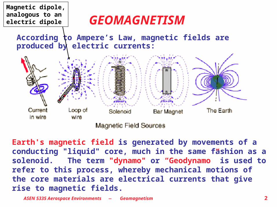
GEOMAGNETISM According to Ampere’s Law, magnetic fields are produced by electric currents:
Earth's magnetic field is generated by movements of a conducting "liquid" core, much in the same fashion as a solenoid. The term "dynamo" or “Geodynamo” is used to refer to this process, whereby mechanical motions of the core materials are electrical currents that give rise to magnetic fields.
Magnetic dipole,analogous to anelectric dipole

ASEN 5335 Aerospace Environments -- Geomagnetism 3
The core motions are induced and controlled by convection and rotation (Coriolis force). However, the relative importance of the various possible driving forces for the convection remains unknown:
• heating by decay of radioactive elements
• latent heat release as the core solidifies
• loss of gravitational energy as metals solidify and migrate inward and lighter materials migrate to outer reaches of the liquid core.
Venus does not have a significant magnetic field although its coreiron content is thought to be similar to that of the Earth.
Venus's rotation period of 243 Earth days is just too slow to produce the dynamo effect.
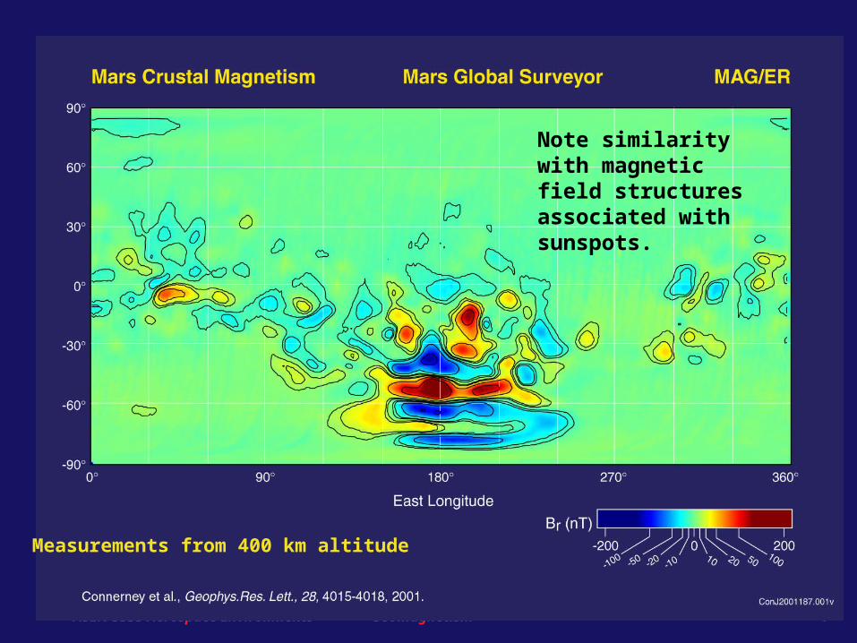
Mars may once have had a dynamo field, but now its most prominentmagnetic characteristic centers around the magnetic anomalies inIts Southern Hemisphere (see following slides).
ASEN 5335 Aerospace Environments -- Geomagnetism 4
Measurements from 400 km altitude
Note similarity with magnetic field structures associated with sunspots.

ASEN 5335 Aerospace Environments -- Geomagnetism 5
• The main dipole field of the earth is thought to arise from a
single main two-dimensional circulation.
• Anomalies of lesser geographical extent (surface anomalies) are field irregularities caused by deposits of ferromagnetic materials in the crust. [The largest is the Kursk anomaly, 400 km south of Moscow].
• Non-dipole regional anomalies (deviations from the main field) are thought to arise from various eddy motions in the outer layer of the liquid core (below the mantle).

ASEN 5335 Aerospace Environments -- Geomagnetism 6
URANUSAxis tilted about 59 degrees and offset from center of planet by 30% of its radius, placing magnetic poles nearer the equator.
NEPTUNEField highly tilted: 47 degrees from rotational axis and offset at least 0.55 radius from physical center of planet.

ASEN 5335 Aerospace Environments -- Geomagnetism 7
The magnetic field at the surface of the earth is determined mostly by internal currents with some smaller contribution due
to external currents flowing in the ionosphere and magnetosphere
In the current-free zone
Therefore
Combined with another Maxwell equation:
Yields
Laplace’s Equation
€
∇× v
B = 1μ
o
J=0
€
vB =−
v ∇V
€
v∇ ⋅
vB =0
€
∇2V =0
ASEN 5335 Aerospace Environments -- Geomagnetism 8
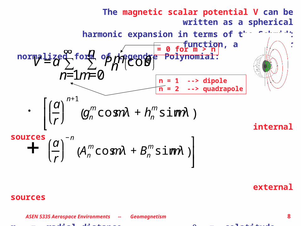
The magnetic scalar potential V can be written as a spherical
harmonic expansion in terms of the Schmidt function, a particular
normalized form of Legendre Polynomial:
internal sources
external sources
r = radial distance = colatitude = east longitudea = radius of earth (geographic polar coordinates)
€
× ar ⎛ ⎝
⎞ ⎠
n+1
gnm cosmλ + hn
m sin mλ( ) ⎡
⎣ ⎢ ⎢
€
+ ar ⎛ ⎝
⎞ ⎠
− n
Anm cosmλ + Bn
m sin mλ( ) ⎤
⎦ ⎥ ⎥
€
V =a Pnmm=0
n∑
n=1
∞∑ cosθ ⎛
⎝ ⎞ ⎠
n = 1 --> dipolen = 2 --> quadrapole
= 0 for m > n

ASEN 5335 Aerospace Environments -- Geomagnetism 9
“magnetic elements”
(H, D, Z)(F, I, D)(X, Y, Z)
Standard Components and Conventions Relating to the Terrestrial Magnetic Field
ASEN 5335 Aerospace Environments -- Geomagnetism 10
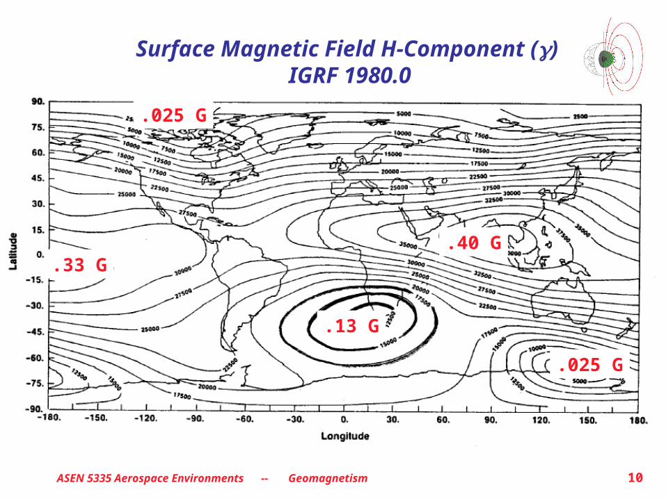
Surface Magnetic Field H-Component () IGRF 1980.0
.13 G
.33 G
.025 G
.40 G
.025 G
ASEN 5335 Aerospace Environments -- Geomagnetism 11
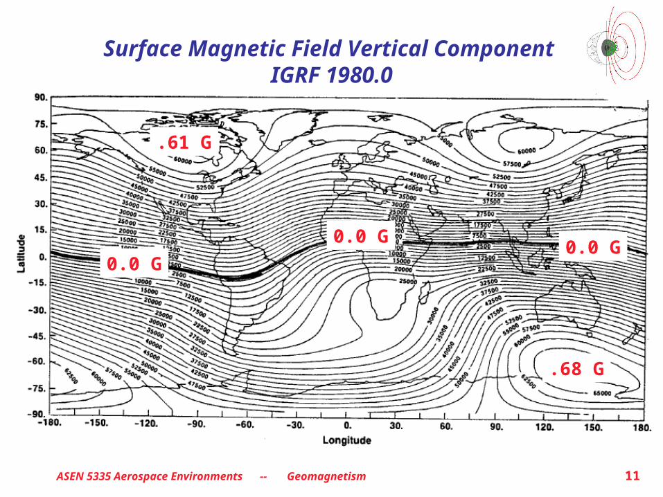
Surface Magnetic Field Vertical Component IGRF 1980.0
0.0 G
0.0 G0.0 G
.61 G
.68 G
ASEN 5335 Aerospace Environments -- Geomagnetism 12
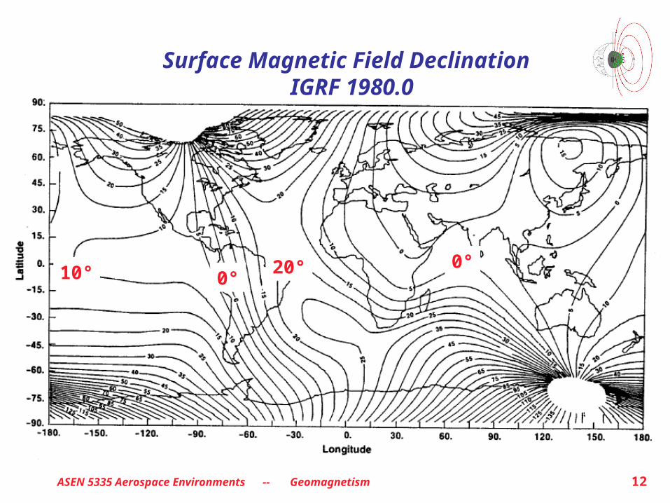
Surface Magnetic Field Declination IGRF 1980.0
10° 20°0°
0°
ASEN 5335 Aerospace Environments -- Geomagnetism 13
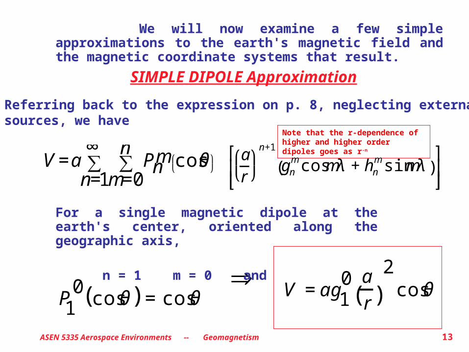
We will now examine a few simple approximations to the earth's magnetic field and the magnetic coordinate systems that result.
€
⇒
€
V = ag10 a
r( )2
cosθ
Note that the r-dependence of higher and higher order dipoles goes as r-n
€
P10
cosθ( ) = cosθ
For a single magnetic dipole at the earth's center, oriented along the geographic axis,
n = 1 m = 0 and
€
V =a Pnmm=0
n∑
n=1
∞∑ cosθ ⎛
⎝ ⎞ ⎠
€
ar ⎛ ⎝
⎞ ⎠
n+1
gnm cos mλ + hn
m sin mλ( ) ⎡
⎣ ⎢ ⎢
⎤
⎦ ⎥ ⎥
Referring back to the expression on p. 8, neglecting externalsources, we have
SIMPLE DIPOLE Approximation
ASEN 5335 Aerospace Environments -- Geomagnetism 14
€
V = ag10 a
r( )2
cosθ
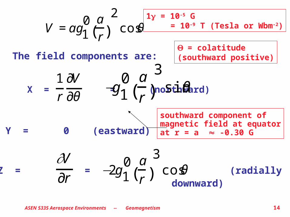
= colatitude(southward positive)
southward component ofmagnetic field at equatorat r = a -0.30 G
1 = 10-5 G = 10-9 T (Tesla or Wbm-2)
€
∂V∂r
€
−2g10 a
r( )3
cosθZ = = (radiallydownward)
Y = 0 (eastward)
The field components are:
X = = (northward)
€
1
r
∂V
∂θ
€
−g10 a
r( )3
sinθ

ASEN 5335 Aerospace Environments -- Geomagnetism 15
A "dip angle", I , is also defined:
=
€
tanI
€
Z
X2 +Y 2= 2cot θ
€
I = tan−1
2 cotθ[ ]
I is positive for downward pointing field
(simple dipole field)
€
X2 +Y 2 +Z 2
€
g10 a
r( )3
1+ 3cos2θ( )1/2
Total field magnitude:
=

ASEN 5335 Aerospace Environments -- Geomagnetism 16
As the next best approximation, let n = 1 , m = 1
We find that
and
where = longitude (positive eastward).
€
P11
cosθ( ) = sinθ
€
V = aa
r( )2
g10 cosθ + g1
1 cosλ + h11sin λ( )sinθ{ }
TILTED DIPOLE Approximation

ASEN 5335 Aerospace Environments -- Geomagnetism 17
Physically, the two additional terms could be generated by two additional orthogonal dipoles placed at the center of theearth but with their axes in the plane of the equator.
Their effect is to incline the total dipole term to the geographic pole by an amount
In other words, the potential function could be produced by a single dipole inclined at an angle to the geographic pole and with an equatorial field strength
This "tilted dipole" is tipped 11.5° towards 70°W longitude and has an equatorial field strength of .312G.
€
= tan−1 g1
1( )
2+ h1
1( )
2
g10( )
2
⎡
⎣
⎢ ⎢ ⎢
⎤
⎦
⎥ ⎥ ⎥
1/2
€
g10
( )2
+ g11
( )2
+ h11
( )2 ⎡
⎣ ⎢ ⎤ ⎦ ⎥
1/2

ASEN 5335 Aerospace Environments -- Geomagnetism 18
It is often more convenient to order data, formulate models, etc., in a magnetic coordinate system. We will now re-write the tilted dipole in that coordinate system rather than the geographic coordinate system.
DIPOLECOORDINATE SYSTEM
Dipole Equator
Dipole latitude Φ
Dipole Axis
(79 , 70 )N W
(79 , 70 )S E
Rotation axis
€
sin Φ = sinϕ sinϕo + cosϕ cosϕo cos λ −λo( )
€
sin Λ =cosϕ sin λ −λo( )
cos Φ= geographic latitude
= geographic longitude = 79°N, 290°E
€
ϕ
€
€
ϕo,λo

ASEN 5335 Aerospace Environments -- Geomagnetism 19
It is often more convenient to order data, formulate models, etc., in a magnetic coordinate system. We will now re-write the tilted dipole in that coordinate system rather than the geographic coordinate system.
DIPOLECOORDINATE SYSTEM
Dipole Equator
Dipole latitude Φ
Dipole Axis
(79 , 70 )N W
(79 , 70 )S E
Rotation axis
€
sin Φ = sinϕ sinϕo + cosϕ cosϕo cos λ −λo( )
€
sin Λ =cosϕ sin λ −λo( )
cos Φ= geographic latitude
= geographic longitude = 79°N, 290°E
€
ϕ
€
€
ϕo,λo

ASEN 5335 Aerospace Environments -- Geomagnetism 20
The above formulation representing dipole coordinates (sometimes called geomagnetic coordinates) is now more or less the same as that for the simple dipole.
Therefore,
in our previous notation = "dipole moment"
= 8.05 ± .02 1025 G-cm3
€
V = −M sin Φ
r2
€
M = g1oa
3
Dipole longitude is reckoned from the American half of the great circle which passes through (both) the geomagnetic and geographic poles; that is, the zero-degree magnetic meridian closely coincides with the 291°E geographic longitude meridian.
€
Φ
€
€
ΛWe will now write several relations in terms of dipole latitude , (instead of geographic colatitude, ) and dipole longitude .

ASEN 5335 Aerospace Environments -- Geomagnetism 21
From the above expression we can derive the following:
€
H =1
r
∂V
∂Φ= −
M cos Φ
r3
€
Z =∂V
∂r=
2M sin Φ
r3
€
tanI =Z
H= −2tanΦ
€
B = H 2 +Z 2 =M
r3 1+3sin2 Φ( )1/2
These look very much like the simple dipole approximation in geographic coordinates.
ASEN 5335 Aerospace Environments -- Geomagnetism 22
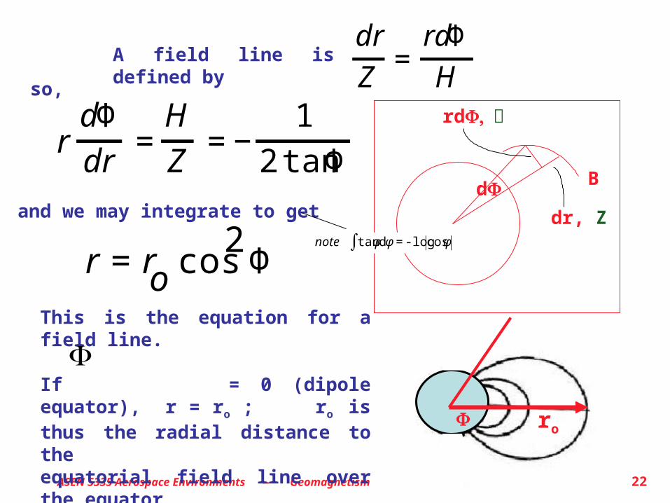
This is the equation for a field line.
If = 0 (dipole equator), r = ro ; ro is thus the radial distance to the equatorial field line over the equator, and its greatest distance from earth.
€
Φ Φ ro
A field line is defined by
€
dr
Z=
rdΦ
H
B
rdΦ
dr, Z
dΦ
€
rdΦ
dr=
H
Z= −
1
2 tanΦ
so,
€
r = ro cos2
Φ
and we may integrate to get
€
note tanφdφ = -logcosφ∫
ASEN 5335 Aerospace Environments -- Geomagnetism 23
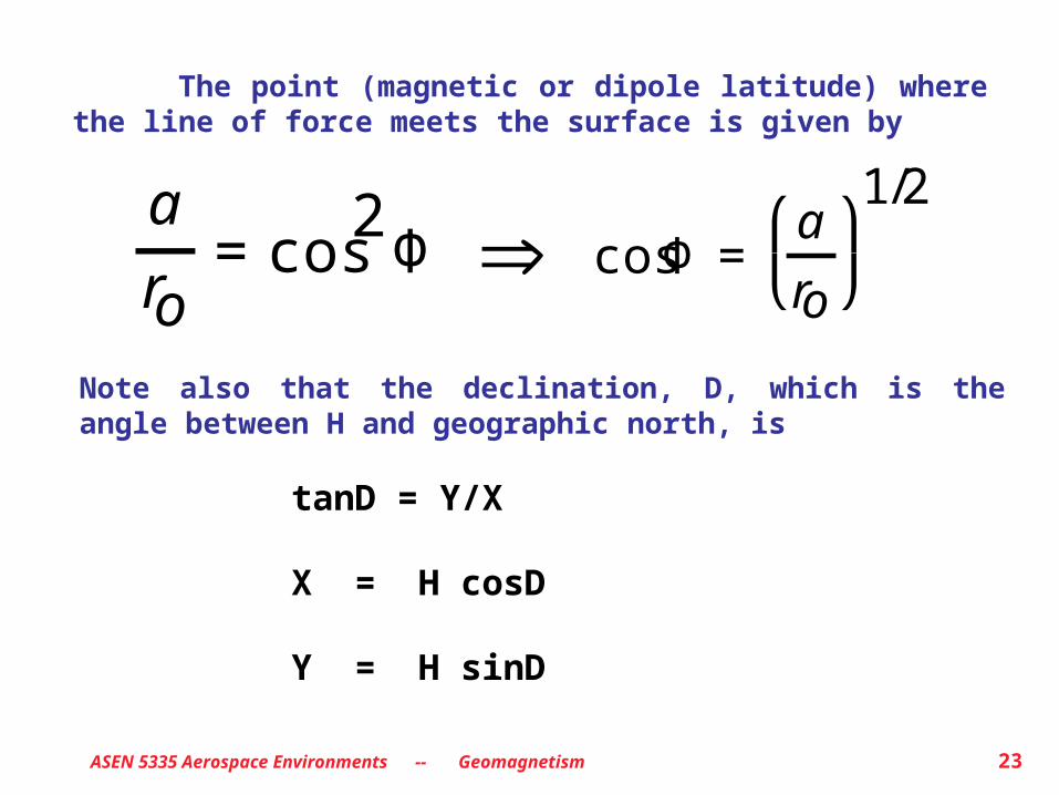
The point (magnetic or dipole latitude) where the line of force meets the surface is given by
€
a
ro= cos
2Φ
€
⇒
€
cosΦ =a
ro
⎛ ⎝
⎞ ⎠
1/2
Note also that the declination, D, which is the angle between H and geographic north, is
tanD = Y/X
X = H cosD
Y = H sinD

ASEN 5335 Aerospace Environments -- Geomagnetism 24
The B-L Coordinate System "L-shells"
Let us take our previous equation for a dipolar field line
and re-cast it so the radius of the earth (a) is the unit of distance.
€
r = ro cos2
Φ
€
R = Ro cos2
Φwhere R and Ro are now measured in earth radii.
Then R = r/a and
€
cosΦ = Ro−1/2
The latitude where the field line intersects the earth's surface (R = 1) is given by

ASEN 5335 Aerospace Environments -- Geomagnetism 25
• Now we will discuss an analogous L-parameter (or L-shell) nomenclature for non-dipole field lines, often used for radiation belt and magnetospheric studies.
• We will understand its origin better when we study radiation belts; basically, the L-shell is the surface traced out by the guiding center of a trapped particle as it drifts in longitude about the earth while oscillating between mirror points.
• For a dipole field the L-value is the distance, in earth radii, of a particular field line from the center of the earth (L = Ro on the previous page), and the L-shell is the "shell" traced out by rotating the corresponding field line around the earth.
• Curves of constant B and constant L are shown in the figure on the next page. Note that on this scale, the L-values correspond very nearly to dipole field lines.

ASEN 5335 Aerospace Environments -- Geomagnetism 26
The B-L Coordinate System:Curves of Constant B and L
The curves shown here are the intersection of a magnetic meridianplane with surfaces of constant B and constant L (The difference betweenthe actual field and a dipole field cannot be seen in a figure of this scale).
ASEN 5335 Aerospace Environments -- Geomagnetism 27
By analogy with our previous formula for calculating the dipole latitude of intersection of a field line with the earth's surface, we can determine an invariant latitude in terms of L-value:
where Λ = invariant latitude
€
cosΛ = L−1/2
Here L is the actual L-value (i.e., not that associated with a dipole field).
Along most field lines L is constant to within about 1% and thus it usefully serves to identify field lines even though they may not be strictly dipolar.


