
ASSESSING THE POTENTIAL OF RAINWATER HARVESTING SYSTEM
AT THE MIDDLE EAST TECHNICAL UNIVERSITY – NORTHERN CYPRUS
CAMPUS
RAYAAN HARB
AUGUST 2015

ASSESSING THE POTENTIAL OF RAINWATER HARVESTING SYSTEM AT THE
MIDDLE EAST TECHNICAL UNIVERSITY – NORTHERN CYPRUS CAMPUS
SUSTAINABLE ENVIRONMENT AND ENERGY SYSTEMS
MIDDLE EAST TECHNICAL UNIVERSITY,
NORTHERN CYPRUS CAMPUS
BY
RAYAAN HARB
IN PARTIAL FULFILLMENT OF THE REQUIREMENTS
FOR
THE DEGREE OF MASTER OF SCIENCE
IN
SUSTAINABLE ENVIRONMENT AND ENERGY SYSTEMS PROGRAM
AUGUST 2015

Approval of the Board of Graduate Programs
_______________________
Prof. Dr. M. Tanju MEHMETOĞLU
Chairperson
I certify that this thesis satisfies all the requirements as a thesis for the degree of Master
of Science
_______________________
Assoc. Prof. Dr. Ali MUHTAROĞLU
Program Coordinator
This is to certify that we have read this thesis and that in our opinion it is fully adequate,
in scope and quality, as a thesis for the degree of Master of Science.
_______________________
Assist. Prof. Dr. Bertuğ AKINTUĞ
Supervisor
Examining Committee Members (First name belongs to the chairperson of the jury and
the second name belongs to supervisor)
Assoc. Prof. Dr. Oğuz SOLYALI, Business Administration,
Jury Chair METU-NCC ________________
Assist. Prof. Dr. Bertuğ AKINTUĞ, Civil Engineering,
Jury Member METU-NCC ________________
Assist. Prof. Dr. İbrahim BAY, Civil Engineering,
Jury Member European University of Lefke ________________

iii
ETHICAL DECLARATION
I hereby declare that all information in this document has been obtained and
presented in accordance with academic rules and ethical conduct. I also declare that,
as required by these rules and conduct, I have fully cited and referenced all material
and results that are not original to this work.
Name, Last Name: Rayaan Harb
Signature:

iv
ABSTRACT
ASSESSING THE POTENTIAL OF RAINWATER HARVESTING SYSTEM
AT THE MIDDLE EAST TECHNICAL UNIVERSITY – NORTHERN
CYPRUS CAMPUS
Harb, Rayaan
M.Sc., Sustainable Environment and Energy Systems
Supervisor: Assist. Prof. Dr. Bertuğ Akıntuğ
August 2015, 142 pages
Rainwater harvesting system (RWHS), where runoff from roofs and
impervious areas is collected and utilized, is a prominent solution to deal with
water scarcity by conserving available water resources and the energy needed to
deliver water to the water supply system. The impact of climate change on water
resources can also be reduced by rainwater harvesting. RWH is becoming an
important part of the sustainable water management around the world. The Eastern
Mediterranean countries with semi-arid climate obtain low precipitation and high
temperature. Therefore, applying RWHS will be very beneficial in these areas to
provide non-potable uses such as irrigation and household use. This study
investigates the potential of RWH in the METU-NCC. Two approaches for runoff
calculation were compared, the traditional Soil Conservation Service (SCS)
method and the Storm Water Management Model (SWMM) using monthly and
hourly rainfall data from 1978 to 2009. A RWHS was proposed to assess the
potential of rainwater harvesting. The reservoir locations of the system were
chosen with their relative irrigation areas and their volumes were calculated after
computing the irrigation consumption of the campus. The study was not aimed at
optimizing the system rather the system serves the purpose to show if there is a
potential in RWH. The tank volumes were found to be 2300 m3, 3500 m3 and 1100
m3 with efficiencies of 37.8%, 41.3% and 90.5% respectively and 41.2% of the
campus irrigation was met. According to the findings, there is potential for
collecting rainwater for irrigation purposes on the campus.
Keywords: Rainwater Harvesting System, Reservoir Volume, Rainfall, Northern
Cyprus

v
ÖZ
ORTA DOĞU TEKNİK ÜNİVERSİTESİ - KUZEY KIBRIS KAMPUSU’NDA
YAĞMURSUYU TOPLAMA SİSTEMİ POTANSİYELİNİN İNCELENMESİ
Harb, Rayaan
Master, Sürdürülebilir Çevre ve Enerji Sistemleri
Tez Yöneticisi: Yrd. Doç. Dr. Bertuğ Akıntuğ
Ağustos 2015, 142 sayfa
Çatılardan ve geçirimsiz yüzeylerden akışa geçen yağmur suyunun toplanarak
kullanılmasını sağlayan yağmursuyu toplama sistemleri, su kıtlığıyla mücadele
kapsamında mevcut su kaynaklarının korunacak olmasından ve ayrıca içme suyu sağlayan
sistemler için gerekli enerjin azaltılacak olmasından dolayı etkin çözüm sağlamaktadır.
Yağmursuyu toplama sistemleri iklim değişikliğinin su kaynakları üzerindeki etkisinin
azaltılmasına da katkı sağlamaktadır. Yağmursuyu toplama sistemleri dünya genelinde
sürdürülebilir su yönetiminin önemli bir parçası olmaktadır. Yarı kurak iklime sahip Doğu
Akdeniz ülkelerinde düşük yağışlar ve yüksek sıcaklıklar gözlenmektedir. Bu bölgelerde
yağmur suyu toplama sistemlerinin uygulanmaya başlamasıyla depolanan su, kullanım ve
sulama suyu ihtiyacına katkıda bulunacaktır. Bu çalışmada ODTÜ-KKK’de yağmursuyu
toplama sistemi kurmak için yeterli potansiyel olup olmadığı araştırılmıştır. Yüzey
akışının hesaplanmasında 1978-2009 yıllarına ait aylık ve günlük yağış değerleri
kullanılarak geleneksel Amerikan Toprak Muhafaza Kurumunun yöntemi ve Yağmursuyu
Yönetimi Modeli (Storm Water Management Model – SWMM ) yazılımı kullanılmıştır.
Yağmursuyu toplama depolarının konumu mevcut yağmursuyu drenaj hatlarına ve her bir
depodan hangi yeşil alanın sulanacağına bakılarak karar verilmiştir. Bu çalışma
kapsamında en uygun sistem ve depo hacmini bulmak için herhangi bir optimizasyon
çalışması yapılmamıştır. Sadece böyle bir sistemin kurulması için yeterli potansiyel olup
olmadığına bakılmıştır. Yapılan çalışma sonucunda kamusa yapılması önerilen 2300 m3,
3500 m3 ve 1100 m3 hacimlerdeki depoların verimlilik oranları sırasıyla %37.8, %41.3 ve
%90.5 olarak elde edilmiştir. Bu çalışmadan elde edilen sonuçlara göre sulama amaçlı
kullanım için kampusa yağmursuyu toplama sisteminin kurulması için yeterli potansiyel
olduğu ortaya çıkmıştır.
Anahtar Kelimeler: Yağmursuyu Toplama Sistemi; Depo Hacmi; Yağış; Kuzey Kıbrıs.

vi
To My Beloved Parents,

vii
ACKNOWLEDGEMENTS
This thesis saw the light with the kind support and help of many individuals. I
would like to extend my sincere thanks to all of them.
Foremost, I would like to express my sincere gratitude to my advisor Assist. Prof.
Dr. Bertuğ Akıntuğ for the support in my Master’s study and research. I would like to
thank my thesis committee Assoc. Prof. Dr. Oğuz Solyalı and Assist. Prof. Dr. İbrahim
Bay for their insightful comments and remarks. In addition, I would like to thank Assoc.
Prof. Dr. Emre Alp for his help and time in answering my questions related to my thesis.
Furthermore, I would like to express my gratitude towards my family, Douraid,
Iman, Lama and Yazan Harb for their unconditional encouragement, patience, motivation
and support throughout my life. Moreover, I would like to thank Eng. Hisham Farook and
Eng. Douraid Harb for their support and guidance that helped me in all the time of research
and writing of this paper.
In addition, I would like to thank all my colleagues and friends for their support
especially Furkan Ercan, Jibran Shahzad, Moslem Yousefzadeh, Azhar Ali Khan, Samer
Al Gharabli, Mohammad Faraj, Riyadh El Alami and Tareq Rabaia for the stimulating
discussions, the sleepless nights we were working together before deadlines, and for all
the fun we have had in the last three years.
Finally, I would like to thank Eng. Huveyda Esen for her time in showing me
around the campus to see the drainage system and the wells in Guzelyurt, as well as Mrs.
Başak Piskobulu for her support and help in finishing this paper.

viii
TABLE OF CONTENTS
ABSTRACT……………………………………………………………………......... iv
ÖZ……………………………………………………………………….……..…….. v
ACKNOWLEDGEMENTS…………………………………….………...………… vii
TABLE OF CONTENTS………………………………………...…………..……. viii
LIST OF FIGURES……………………………….……………...………………….. x
LIST OF TABLES…………………………………………..……………..…......... xii
LIST OF SYMBOLS AND ABBREVIATIONS………………………………..... xiii
CHAPTER I: INTRODUCTION……………………………………….…...…..…... 1
1.1 Statement of the Problem………….…………………...…………………... 1
1.2 Objective of the Study………………….………………………...……….... 2
1.3 Organization of the thesis……………….………………………………….. 2
CHAPTER II: LITERATURE REVIEW…………….……………………………… 3
2.1 Rainwater Harvesting Systems………………….……………...…………... 3
2.2 Studies about Rainwater Harvesting Systems……….…………………..….. 5
2.3 Rainfall Runoff Methods…………………....………….…………………… 15
2.4 Water Storage Tanks………………………….……………...………...…… 20
2.4.1 Dry Period Demand Method………………….……………..……...…. 27
2.4.2 Simple Method……………………………………….…………...….... 27
2.4.3 Simple Tabular Method……………………………………..……...….. 27
2.4.4 Graphical Method……………………………………….…….….……. 28
CHAPTER III: DESCRIPTION OF STUDY AREA………………………………... 29
3.1 Overview of the Case Study……..……………………....…………………..…. 29

ix
3.2 Description of the Site………………………..……….………...……….….... 31
3.3 Soil Characteristics……………………………….…………..…..........…….. 36
CHAPTER IV: DATA AND METHODOLOGY……….............................................. 38
4.1 Precipitation Data……………………………………………...………….….. 38
4.2 Catchment Area……………..………………………………....……...….…... 40
4.3 Traditional SCS Method.…………………………………...…….…….…….. 42
4.4 SWMM Model…………………………………………...………….…….….. 44
4.5 Irrigation Demand……………………………………...…………….….……. 51
4.6 Location of Reservoirs……………………………...…………………..…….. 54
4.7 Tank Size Calculation Method…………………...……………………..…….. 59
CHAPTER V: CALCULATIONS, RESULTS AND DISCUSSION……………….… 61
5.1 Catchment Area…………………………………………...……….…….….… 61
5.2 Catchment Runoff…………………..…………………….………………..…. 61
5.2.1 Traditional SCS Results……...…………………………………….……. 62
5.2.2 SWMM Model Results……………………...………………………….... 63
5.2.3 Sensitivity Analysis………………………………...……………….....… 66
5.3 Irrigation Requirements……...…………………………………………….…. 71
5.4 Water Tank Sizing Results………..…………………………………….……. 73
CHAPTER VI: CONCLUSION…………………..…………………………………... 81
REFERENCES………………………………………………………..…………...….. 83
APPENDIX A………………………………………………………………………… 89
APPENDIX B………………………………………………………………………… 93
APPENDIX C………………………………………………………………………… 140

x
LIST OF FIGURES
Figure 2.1. Pressure at the bottom of a tank……………………………………………. 20
Figure 2.2. Pressure distribution and 3-D representation on a vertical wall………...…. 21
Figure 2.3. Amount of reinforcement against tank capacity……………………...……. 21
Figure 2.4. Amount of concrete against tank capacity...……………………………….. 22
Figure 2.5. Amount of formwork against tank capacity…………………...…………... 22
Figure 2.6. Tensile stress in the rectangular concrete tank…………………………...... 23
Figure 2.7. Tensile stress in the cylindrical configuration……………………………... 23
Figure 3.1. Map of Cyprus……………………………………………………….…...... 28
Figure 3.2. Top view of METU-NCC………………………………………………….. 31
Figure 3.3. The different surfaces present on campus …………..………………...…… 33
Figure 3.4. Plan of METU-NCC ……………………………………….…………...…. 35
Figure 3.5. HWSD viewer window………...…………………………………………... 36
Figure 3.6. Map of Cyprus in the HWSD viewer……………………………...……….. 36
Figure 4.1. Average monthly rainfall from Guzelyurt station….....……………………. 38
Figure 4.2. Annual rainfall versus water year from the Guzelyurt station………..……. 38
Figure 4.3. The percent distribution of daily rainfall in Guzelyurt………………….…. 39
Figure 4.4. Plan of METU-NCC with different sub-catchments colored..…...………... 41
Figure 4.5. The SWMM runoff/routing flow in a sub-catchment…………..……...…... 46
Figure 4.6. The sub-catchment editor and infiltration editor windows in SWMM…….. 47
Figure 4.7. The junction, conduit and outfall editor windows on SWMM respectively.. 49
Figure 4.8. The rain gage and time series editor and the rainfall data format…….……. 49
Figure 4.9. The appearance of the SWMM model…………………….……………...... 50
Figure 4.10. The simulation dates options window…………………………...………... 50
Figure 4.11. The three groups of vegetation on campus……………………………….. 51
Figure 4.12. The AutoCAD map showing the vegetation on the campus……………… 53
Figure 4.13. The map with reservoir locations and irrigation areas on campus………... 55
Figure 4.14. The area that Reservoir 1 irrigates……………………………………...… 56
Figure 4.15. The area that Reservoir 2 irrigates……………………………………...… 57
Figure 5.1. The effect of change in soil drying time on runoff in sub-catchment 1……. 67
xi
Figure 5.2. The effect of change in soil drying time on runoff in sub-catchment 2…..... 68
Figure 5.3. The effect of change in soil drying time on runoff in sub-catchment 3…..... 68
Figure 5.4. The effect of change in soil drying time on runoff in sub-catchment 4…..... 69
Figure 5.5. The effect of change in soil drying time on runoff in sub-catchment 5…..... 69
Figure 5.6. The effect of change in soil drying time on runoff in sub-catchment 6…..... 70
Figure 5.7. The effect of change in soil drying time on runoff in sub-catchment 7…..... 70
Figure 5.8. The effect of change in soil drying time on runoff in all sub-catchment during
the peak monthly rainfall…………………………………………………….................. 71
Figure 5.9. The annual and average water tank volume of Reservoir 1........................... 74
Figure 5.10. The annual and average water tank volume of Reservoir 2…………......... 76
Figure 5.11. The annual and average water tank volume of Reservoir 3………….…… 76
Figure 5.12. The storage system with a first flush tank and a sedimentation tank…...… 78
Figure 5.13. Modular Tank System…………………………………………...………... 80

xii
LIST OF TABLES
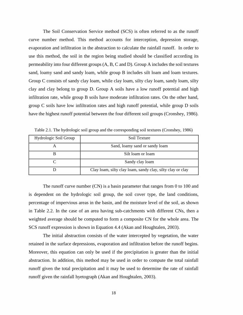
Table 2.1. The hydrologic soil group and the corresponding soil textures…………….. 18
Table 2.2. Runoff Curve Numbers for urban land uses ……………………....……...... 19
Table 2.3. The pros and cons of above-ground versus underground water tanks…..….. 25
Table 2.4. The advantages and disadvantages of different storage tank materials…...... 26
Table 3.1. Soil data from the HWSD viewer of the location specified on the map…..... 37
Table 4.1. The crop type along with the irrigation requirements on each type ………... 52
Table 4.2. The reservoirs, the sub-catchments supplying their runoff and the
corresponding irrigation areas.………………..........................................................…... 54
Table 5.1. Areas (m2) of every surface in each sub-catchment………………..……….. 61
Table 5.2. The data used in the spreadsheet SCS method………………….…………... 62
Table 5.3. Spreadsheet monthly runoff volume (m3) from each sub-catchment…....….. 63
Table 5.4. The input data in the SWMM model for all the sub-catchments………...…. 64
Table 5.5. Daily rainfall data (mm) of days 1 to 10 in each month of 1978 ….......….... 64
Table 5.6. Hourly rainfall (mm) data for the first ten days of January 1978……...…… 65
Table 5.7. SWMM monthly runoff volume (m3) from each sub-catchment…...……… 66
Table 5.8. The areas occupied of each crop type in the seven sub-catchments…...…… 72
Table 5.9. The monthly water consumption (m3) of each sub-catchment……………... 72
Table 5.10. The monthly water consumption (m3) of the three irrigation areas…...…... 73
Table 5.11. Reservoir volumes and corresponding percent demand met…………….... 74
Table 5.12. The water balance during 1986-1987 to find the volume of Reservoir 1…. 75
Table 5.13. Annual water demand and annual saving………………………………….. 77

xiii
LIST OF SYMBOLS AND ABBREVIATIONS
𝐴𝑖 Area of each surface in a sub-catchment
𝐴𝑇 Total area of sub-catchment
AHP Analytical Hierarchy Process
CAS Chinese Academy of Sciences
CCC Culture and Convention Center
𝐶𝑁 Curve Number
𝐶𝑁𝑁 Normalized Curve Number
𝐶𝑆 Cumulative Surplus
𝐷 Water demand
𝐷𝑀 Demand Met
𝐸 Water saving efficiency
EPA Environmental Protection Agency
𝑓 Actual rate of infiltration
𝑓𝑝 Infiltration capacity
FAO Food and Agriculture Organization of the United Nations
HWSD Harmonized World Soil Database
𝑖 Rate of precipitation
𝐼𝑎 Initial abstraction
IIASA International Institute for Applied Systems Analysis
IT Information Technology
ISRIC International Soil Reference and Information Centre
JRC Joint Centre of the European Commission
METU-NCC Middle East Technical University- Northern Cyprus Campus
𝑃 Precipitation
𝑅 Rainfall runoff
RWHS Rainwater Harvesting System
𝑆𝐷 Soil moisture deficit at time of runoff

xiv
𝑆𝐶 Storage Capacity
SCS Soil Conservation Service
SP Spillage
𝑉 Volume of rainwater
𝑊𝑆 Water Storage

1
CHAPTER I
INTRODUCTION
1.1 Statement of the Problem
Cyprus is the third largest island in the Mediterranean Sea with an area of 9,251
km², the island experiences hot and dry summers while winters are mild (T.C. Başbakanlık
Yayınları, 2000). The island witnesses a problem of water scarcity mainly due to low
annual precipitation and unfavorable distribution of annual rainfall. Moreover,
groundwater is being depleted and the quality of groundwater has reduced due to over-
pumping of the aquifers leading to the entry of saltwater (Priscoli and Wolf, 2009).
Therefore, an approach of supplying water from Turkey was adopted (Priscoli and Wolf,
2009). An approach to collect and utilize the rainwater that is discarded by urban drainage
systems can provide an annual supply of water to sustain the irrigation demands in a
specific area. The hydraulic system that applies this approach is called rainwater
harvesting system (RWHS). Conventionally, urban rainwater management considered
rainwater runoff as a waste to be guided away in a controlled manner. Collection of rainfall
runoff grants an adequate supply of water for ample uses whether outdoor or indoor.
Moreover, rainwater harvesting system reduces effects of urbanization such as flooding,
erosion and pollution problems. This leads to the statement that rainwater is a resource
that can be stored and used.
Rainwater harvesting is not a new concept, it was applied as early as 4500 B.C. by
the inhabitants of southern Mesopotamia (present day Iraq) and by other inhabitants of
different regions in the Middle East. The Romans later developed the primitive rainwater
harvesting systems into more sophisticated systems in order to irrigate their lands
(Sivanappan, 2006). Moreover, rainwater harvesting systems were also employed in
ancient Persia, where large underground cisterns were deployed to store the surface
runoff; remains of these cisterns are still visible (Pazwash, 2011). There are ample
objectives of rainwater harvesting systems that include directing storm water runoff to
natural depressions or reservoirs. Moreover, this water can be used for irrigation,
supplying household water, supplying drinking water and injecting this water into the
ground to replenish groundwater supply (Pazwash, 2011). Furthermore, in-situ rainwater

2
harvesting systems may reduce the carbon footprint of water collection and the
distribution cycle, as well as reducing the cost of water transportation (Zuberi et al., 2013).
1.2 Objective of the study
The main objective of this study is to assess the potential of rainwater harvesting
on the campus of the Middle East Technical University - Northern Cyprus (METU-NCC)
and to propose a rainwater harvesting system that can provide water for irrigation.
Moreover, this system should easily be integrated with the existing system. Although this
study focuses on the METU-NCC, the findings of this work may be implemented in
different locations of Cyprus as well as countries with similar climate as Cyprus.
1.3 Organization of the thesis
The study commences with an introduction including a statement of the problem,
objectives and purpose as well as the methods used in the study. The second chapter
comprises of the background literature. Then, the third chapter describes the site of
METU-NCC; the area, existing water consumption and the systems used to supply non-
potable water. In the fourth chapter, the methodology of the study, and data used to
calculate the monthly rainwater runoff and the water tank calculations will be presented.
The fifth chapter discusses the results of the runoff and the water tank volumes as well as
the location of the tanks and the integration of the rainwater harvesting system with the
existing system. Finally, the paper is concluded including the future modifications to the
rainwater harvesting system and the future research possibilities are addressed.

3
CHAPTER II
LITERATURE REVIEW
2.1 Rainwater harvesting systems
Rainwater harvesting is defined as collecting from catchment areas such as roofs
or other urban structures to meet demand for domestic, industry, agriculture, and
environmental purposes when water sources are becoming scarce or low quality
(Aladenola and Adeboye, 2009; Hamid and Nordin, 2011; Worm and Hattum, 2006). This
process has been used by ancient civilizations for agricultural irrigation and as a source of
drinking water and this allowed those civilizations to flourish in semi-arid regions.
Nowadays, RWHS are being used in water-limited locations, such as western U.S. regions
and in some African countries in order to provide potable water, household water as well
as for irrigation (Ling and Benham, 2014). Moreover, RWH is used as a method of urban
flood control through redirecting the rainwater away from regions of low water drainage.
Collecting and using rainwater may decrease the use of municipal and
groundwater. Since the rainwater collected from roofs is relatively cleaner than the
rainwater collected from other impermeable surfaces such as roads, roofs are the largest
impervious surface in residential areas to be used as catchment areas and allow the harvest
of water that would otherwise enter into the storm-water drainage system. This may reduce
storm-water runoff and the necessity for downstream storm-water management and
treatment. Rainwater is clean as it falls, but the surface that this water is collected from
contains the contaminants, therefore necessary treatment and filtration is needed before
storing this water. Harvested rainwater is used mainly for irrigation and toilet flushing
(Ling and Benham, 2014).
According to Hamid and Nordin (2011), there are six components of any RWHS:
I. Catchment area
II. Gutters and downspouts
III. Filtration system
IV. Storage system
V. Delivery system
VI. Treatment system

4
The quantity of rainwater that can be collected from a surface such as a roof is
dependent on its size and texture. Moreover, the material of the catchment surface will
affect the rainwater quality through the contaminants that might be present on the surface
(Ling and Benham, 2014).
The gutters and downspouts will lead the rainwater from the catchment surfaces
to the storage system. The purpose of the filtration system is to prevent the flow of debris
from the surfaces to the pipes of the storage system. This can be done by installing screens
that can accumulate the debris and may be cleaned manually. The size and material of the
debris will dictate the size of the screens. Moreover, leaf guards can be installed to prevent
the entry of leaves to the pipes. An important part of the filtration system is the first “flush”
removal. The first flush of rainwater will contain material that has collected on the
catchment surface since the last rainfall event, which may include dust, pollen, leaves,
insects, bird feces, and other residues (Ling and Benham, 2014). It is recommended to
divert from 0.2 mm to 2 mm of the runoff as first flush depending on the quality of water
(Doyle, 2008).
The storage system is usually the largest investment aspect of the rainwater
harvesting system. Therefore it requires careful analysis to provide the optimal storage
capacity and structural durability at the lowest possible cost. Storage reservoirs are in two
categories: surface and sub-surface storage tanks (Worm and Hattum, 2006). The water
reservoir may be constructed from many different materials that include fiberglass,
polypropylene, concrete or metal. Cisterns should be made to inhibit algal growth and
they should be screened to prevent mosquito breeding. Furthermore, they should be
cleaned regularly to ensure the cleanliness of the stored water (Ling and Benham, 2014).
In the systems intended for non-potable uses such as irrigation and toilet flushing,
screens and first flush diverters are sufficient for treatment thereby reducing the cost of
the system. On the other hand, potable use of the collected rainwater will require treatment
and disinfection to remove contaminants and toxins in order to meet drinking water
standards (Ling and Benham, 2014).

5
2.2 Studies about Rainwater Harvesting Systems
In a study conducted by Zuberi et al. (2013), the theoretical potential of rainfall at
METU-NCC was studied to supply water for toilet flushing in the dormitories. It was
found that a RWHS installed to collect rainwater from the roof areas of the three
dormitories present would be sufficient for the flushing consumption of the second
dormitory. 2831 m3 of water can be collected annually with a reliability of 93%. This study
showed that there is an opportunity for water scarce areas to utilize their limited resources
in an efficient way.
A study was conducted by Dwivedi et al. (2013) to estimate the rooftop harvesting
potential of the buildings as well as the planning and designing of the RWHS, the delivery
system, and the groundwater recharge system. This study is performed for the Dhule town
in India and a 50 mm/hr rainfall intensity was assumed for the modelling of this system.
Moreover, the cost of different components of the system was studied and an annual
equivalent capital cost was estimated. The unit cost of water appeared to be high in
comparison to the market price, however, the environmental benefits of the groundwater
recharging with good quality water validates such projects.
Hamid and Nordin (2011) selected a male residential college in Malaysia to
perform their case study in order to determine the reliability of rainwater harvesting
system installation. Malaysia receives about 3000 mm of rainfall annually. Moreover, this
study illustrates that 90% reliability may be achieved based on the rainfall data and roof
catchment area of the college and it was estimated that the system would save RM 10460
(3275.40 USD) annually on the water bill.
In another research conducted for Abeokuta, Nigeria, by Aladenola and Adeboye
(2009) showed that rainwater harvesting systems can satisfy the monthly water
consumption for toilet flushing and laundry except for the months from November till
February. Abeokuta has a mean annual rainfall of 1156 mm. Moreover, provided there is
sufficient rainfall, the excess rainwater stored during September and October is adequate
to supply water during the dry months.
Furumai et al. (2008) conducted a study to explain the trend of promotion of
rainwater storage and harvesting in Japan with an estimated average annual total
precipitation of 640 billion m3, after evapotranspiration leaving a potential of 410 billion

6
m3 of water to be utilized for industry, household and agriculture. Moreover, this paper
further emphasizes that there are different uses of this water. A new type of rainwater use,
which is water supply to heated road surface, is highlighted. This was introduced to
diminish the urban heat-island phenomena. Moreover, this paper introduces research on
detailed land-cover classification of rooftops using satellite image and GIS data, this is
beneficial for advanced urban runoff simulation and for estimation of potential of
rainwater storage and harvesting facilities.
In a research conducted by Jothiprakash and Sath (2009) different RWH
techniques were evaluated to identify the most appropriate method for a large-scale
industrial area in Maharashtra, India, to satisfy its daily water demand. The industry is
located in an area that receives an average annual rainfall of 2983 mm. Moreover, the
volume of water to be stored was determined through mass balance method, Ripple
diagram method, analytical method and sequent peak algorithm method. Then Analytical
Hierarchy Process (AHP) was used to determine the most appropriate type of RWH
technique and the required number of RWH structures. The results showed that AHP can
be a useful tool to evaluate RWH methods and structures.
The Department of Water in Perth, Australia, conducted a study to evaluate the
potential use of storm water in Perth. The storm water discharge was estimated as rainfall
over the percentage of impervious surface that drains to the environment. The study
indicated that a significant volume of water is generated in the region and could be
harvested as a potable or non-potable water supply. The water can be pumped to infiltrate
or injected into the superficial aquifer for storage (Department of Water, 2008).
In a study performed in Tehran, Iran by Mehrabadi and Motevalli (2012) on the
operation of rooftop rainwater harvesting systems to reduce urban flood, have found that
by collecting the rainfall runoff from residential rooftops, urban flood control can be
attained. Tehran has an average annual rainfall of 238.9 mm, and by modelling different
tank volumes to collect rooftop runoff, it was found that with increasing tank size and
subsequently the volume of collected water, the urban flood frequency decreased.
Tobin et al. (2013) performed a study on the assessment of rainwater harvesting
systems in the rural area of Edo State in Nigeria. They collected data using quantitative
data collection methods such as a survey questionnaire, checklist and bacteriological

7
assessment of water quality. The data was analyzed using the statistical package for social
sciences and the results showed that the rooftop rainwater harvesting was used by over
80% of the households. The stored water was mainly utilized for personal hygiene
purposes. The water samples tested showed an unacceptable levels of coliforms and E.
coli bacteria.
Nafisah and Matsushita (2009) conducted a comparative study on the metropolis
rainwater harvesting practices Sumida-Ku in Tokyo, Japan and Selangor, Malaysia. The
paper states that the rainwater harvesting systems in Tokyo are well developed and this
technique has started few decades ago, while in Malaysia they are behind in implementing
the rainwater harvesting systems. The paper discusses and compares the policy and
planning, design and social issues attributed to the rainwater harvesting systems in Japan
and Malaysia. Moreover, the aspects implemented in Japan that Malaysia should work on
to improve and adopt are shown.
A research conducted by Grady and Younos (2008) analyzed the water and energy
conservation of rainwater harvesting system on a single family house. They have analyzed
and compared the efficiency of two water systems, a local groundwater and rainwater
harvesting systems. This residence is located in Montgomery County, Virginia in the
United States. The rainwater harvesting system collects water from the rooftop runoff and
stores this water in an underground storage tank. The rainwater is utilized for outdoor and
indoor purposes as well as for potable use. The rainwater harvesting system exhibited a
supply of 84% of the water consumption of the household with an average annual rainfall
of 987.6 mm. Moreover, the study showed that for this case the groundwater system was
more efficient and cost-effective but both systems were more cost-effective and energy
effective than extending a public water line to the residence.
A field study performed by Strand (2013) to show how rainwater harvesting
systems in the urban areas of Colombo, Sri Lanka, can act as a solution for sustainable
water management issue and that this system might lead to economic and environmental
advances. The aim of this study was to find solutions to improve the water management
in Sri Lanka. Moreover, the annual rainfall in Sri Lanka is between 2500 to 5800 mm in
the south west region of the island and about 1250 mm in the other regions of the island.
The rain often comes in short heavy bursts causing floods. Furthermore, the result of the

8
field study showed that the economic and environmental benefits associated with
rainwater harvesting systems are possible sustainable solutions to the water issues on the
island. In addition, this study opts to illustrate the areas where the rainwater harvesting
systems have the best potential with the highest impact.
A report prepared by the Maryland Department of the Environment provides a
summary on the development and calibration of a watershed model for the Patapsco/Back
River Watershed using the SWMM software. This report includes sections on the
watershed properties, model structure, development and calibration. The report discusses
the watershed from the hydrological and water quality perspectives. Two precipitation
gauges were used and the simulation was performed from 1/1/1992 to 9/31/2001 and
results showed the infiltration rate and runoffs in the basin as well as pollutant transport
such as heavy metals in the watershed (Maryland Department of the Environment, 2002).
Nnaji and Mama (2014) conducted a study to assess the potential for rainwater
harvesting in Nigeria to focus on flood mitigation and domestic water supply. This work
was done by using 26 locations in the major ecological zones of Nigeria and classifying
residential buildings into different classes with different amounts of water consumption.
A water balance approach was utilized for each class to evaluate the fraction of water
demand that can be satisfied by the rainwater and so defining the minimum water storage
capacity to be used. Results illustrated that for the reliability of system was over 80 % for
the rainforest and guinea savanna zone. Monthly precipitation data between 17 and 30
years were used for each location and the average coefficient of variation of this was
calculated and the results showed that the rainwater harvesting potential was a power
function of rainfall coefficient of variation.
Zura, a village in India has scarce water resources that are under threat due to
droughts, increasing ground water salinity and groundwater over-exploitation. A study
was conducted as an attempt to assess the potential of rainwater harvesting in this village
with an average annual rainfall of 332 mm. The results found in this research is that a
decentralized management strategy of the rainwater is greatly needed in order to make the
people self-dependent in obtaining their drinking water requirements (Tripathi and
Pandey, 2005).

9
Another study in Kanai, Mali, was performed to determine the rate of water
consumption and current water sources in order to estimate the volume of rainwater that
can be collected using questionnaires administered to households. Questions related to the
socio-economic state of households, source of water, methods of rainwater harvesting and
purpose of use of the water were asked in the questionnaires. A survey suggested that
more than half of the households depend on sources that are susceptible to drought while
only 3 % of them utilize rainwater. The study area has an average annual rainfall of 1064
mm and the amount could not satisfy the water consumption if the present techniques are
not improved by increasing the involvement of the villagers (Lekwot et al., 2012).
Ward et al. (2010) evaluated the design of two different rainwater harvesting
systems using an advanced continuous simulation model. The systems illustrated between
36% and 46% of the WC demand. Moreover, the simple tank design methods resulted in
larger tank sizes compared to the simulation model. This has led to an over-sizing in the
tanks installed. The catchment size, a parameter neglected in the simple method, was
found to be important in tank sizing. Furthermore, a cost analysis was conducted and it
was found that the rainwater harvesting systems are more feasible in large commercial
buildings compared to smaller domestic systems.
Rahman et al. (2012) investigated the water savings potential of rainwater tanks
installed in 10 houses in different locations in Sydney, Australia. Three different tank sizes
were studied, 2 kL, 3 kL and 5 kL, using a water balance simulation model. The analysis
was conducted on a daily time scale and the water saving, reliability and cost feasibility
were observed. The findings of the study showed that the average annual water saving
was correlated with the average annual rainfall, while the benefit cost ratios for the
rainwater tanks were less than 1.00 without government support. The study noted that the
5 kL tank was a better option than the 2 kL and 3 kL tanks. The rainwater tanks should be
supply water to the toilet, laundry and outdoor irrigation to attain the best financial
outcome for the users. The results of this study propose that government authorities should
maintain or increase the financial support for rainwater tanks.
Since the water balance of RWHS is dominated by the stochastic nature of
precipitation. Unami et al. (2015) developed a mathematical model containing stochastic
differential equations, with model parameters that can be recognized from observed data

10
to explain the dynamics of RWHS for irrigation. Stochastic control problems were
expressed and then solved to find the optimal irrigation approaches during the dry season.
The same procedure may be inversely applied to design the system dimensions. The model
parameters were identified with the observed data in an experimental micro RWHS in
Japan and in the semi-arid savanna in Ghana. Finally, a real life RWHS that will be
employed in the Jordan Rift Valley was discussed.
Imteaz et al. (2012) developed a simple spreadsheet based daily water balance
model to assess the performance and design of rainwater tanks. Daily rainfall data, roof
catchment area, rainfall loss factor, available storage volume, tank overflow and water
demand were used in the analysis. Moreover, this model was used to design the optimum
size of domestic rainwater reservoir in southwest Nigeria for the dry months. Two demand
situations were evaluated, the first was toilet flushing only and the second was toilet
flushing and laundry use. The results of this study were compared with results from earlier
studies, which used monthly average rainfall data. It was found that the analysis using
monthly average rainfall data over-estimates the rainwater tank volume. This study
showed 100% reliability with a tank volume of 7 m3 during low demand, however, during
higher demand a larger tank volume of 10 m3 was required to obtain 100% reliability.
Furthermore, the large quantities of water was lost as overflow, with a tank size of 10 m3,
therefore, the collected rainwater could be used for other purposes if large tanks were to
be installed.
Imteaz et al. (2011) conducted a study on the evaluation and design of rainwater
tank for large roof areas in Melbourne, Australia, using daily rainfall data representing
three different climatic scenarios dry, average and wet years. The average annual rainfall
in Melbourne is 650 mm. A spreadsheet-based daily water balance model was developed
considering the daily rainfall data, the roof areas, the rainfall loss factor, the available
storage volume, the tank overflow and the irrigation demand. Two underground rainwater
tanks were considered, 185 m3 and 110 m3. Using the model, the reliability of each tank
under different climatic regimes was examined. The results showed that both the tanks
were reliable in wet and average years but less effective during the dry years. A payback
period analysis showed that the total construction cost of the tanks can be recovered within
15 to 21 years taking into account the tank size, climatic conditions and future water price.

11
Moreover, a correlation between the water price increase rates and payback periods was
developed. The study emphasizes the importance of optimization and cost analysis for
large rainwater tanks in order to maximize the benefits.
Al-Ansari et al. (2012) conducted a study on the Sinjar area of northwest Iraq, with
an average annual rainfall of 320 mm, by applying RWH modeling methods for
agricultural purposes. Linear Programming optimization and Watershed Modeling
System methods were used to increase the irrigated area. The methods employed
demonstrated to be effective for solving large-scale water demand issues with multiple
parameters. Two scenarios were studied, the first scenario was that each reservoir operated
as an individual unit while, the second was that all reservoirs in the basin operated as one
system. The two scenarios illustrated positive results but the second scenario provided
better results than the first.
The utilization of non-dimensional parameters was proposed in a study conducted
by Palla et al. (2011) in order to investigate the optimum performance of RWHS. A model
was applied to evaluate the inflow, outflow and change in storage volume of a RWHS
using a daily mass balance equation; the water-saving efficiency, over-flow ratio and
detention time were determined and utilized to measure the system performance over a
long-term simulation period. Different scenarios were examined to test the system
performance, three precipitation regimes, three levels of water demand and ten storage
capacity levels. The demand fraction and the storage fraction were the two non-
dimensional parameters used to investigate the optimum sizing of the RWHS. The demand
fraction was found to affect the water-saving efficiency and the overflow ratio, while the
storage fraction affects the detention time which influences the water quality degradation
in the system. A sensitivity analysis was conducted to examine the effect of the length of
the time series climate records on the reliability of the selected performance indices. The
results showed that 30 years of daily rainfall records are adequate for assessment of the
system performance.
Since there is a great variation in average annual rainfall between the east and west
of Greater Melbourne, ranging from 1050 mm in the east and 450 mm in the east, then
there is a difference in rainwater tank size to satisfy similar demands and to provide the
same supply reliability. Khastagir and Jayasuriya (2010) presented a novel procedure and

12
a correlation for the optimal sizing of rainwater tanks taking into account the annual
rainfall, the demand for rainwater, the catchment area and the supply reliability. The
developed dimensionless curve reflects these variables and sets the path for developing a
web-based interactive tool for choosing the optimum rainwater tank size.
Basinger et al. (2010) assessed the reliability of using harvested rainwater as a
means of flushing toilets, irrigating gardens, and topping off air-conditioner in residential
buildings in New York City by utilizing a new RWHS reliability model. The model can
be is not case specific since it is based on a non-parametric rainfall generation method
using a bootstrapped Markov chain. The RWHS reliability is determined for user-
specified catchment area and tank volume ranges using precipitation generated using the
stochastic procedure. The reliability with which backyard gardens and air conditioning
units are supplied with rainwater exceeded 80% and 90%, respectively, while toilet
flushing demand can be met with a 7–40% reliability. When the reliability curves
developed were utilized to size RWHS to flush the low flow toilets, it was found that the
rooftop runoff to the sewer system was reduced by about 28% over an average rainfall
year, and the potable water demand was decreased by about 53%.
Abdulla and Al-Shareef (2009) evaluated the potential for potable water savings
by using rainwater in residential areas of the twelve Jordanian districts and proposed
methods to improve both quality and quantity of harvested rainwater. The rainfall varies
from 600 mm to less than 200 mm annually over the twelve districts. The results showed
that a maximum of 15.5 Mm3/y of rainwater can be collected from the roofs of residential
buildings assuming that all surfaces are utilized and all the rainfall on the surfaces is
collected. The estimated collected rainwater is equivalent to 5.6% of the total domestic
water supply of the year 2005. The potential for RWH varies between the districts, ranging
from 0.023×10⁶ m3 to 6.45×10⁶ m3, while the estimated potential for potable water
savings, ranged from 0.27% to 19.7%. Samples of harvested rainwater from residential
roofs were analyzed; the measure of inorganic compounds matched the World Health
Organization standards for drinking water, while fecal coliform, an important
bacteriological parameter, exceeded the limits for drinking water.

13
Ghisi (2009) analyzed the effect of rainfall, roof area, number of residents, potable
water demand and rainwater demand on rainwater tank sizing. Computer simulation was
used for the analysis, considering daily rainfall data for three cities in the state of São
Paulo, Brazil. The roof areas considered were 50, 100, 200 and 400 m2, the potable water
demands were 50, 100, 150, 200, 250 and 300 L per capita per day, while the rainwater
demands were taken as a percentage of the potable water demand and the number of
residents was considered to be two or four. The results showed a broad variation of
rainwater tank sizes for each city and for each parameter. Hence, the conclusion of the
study is that rainwater tank sizing for houses must be performed for each specific situation,
taking into account the local rainfall, roof area, potable water demand, rainwater demand
and number of residents.
Santos and Taveira-Pinto (2013) carried out a study to describe and analyze six
different calculation methods for rainwater tank sizing. In order to apply these methods,
two cases of RWHS were utilized, a dwelling and a public building. The results indicated
that the methods based on the maximum rainwater demand and 100% efficiency
conditions lead to an over-estimation of the rainwater storage tanks, thus need long
payback periods. Moreover, daily simulation at 80% efficiency was the most suitable
condition to size the RWHS, since it led to the best ratio of economic savings/installation
cost. Furthermore, the Rippl method and the 80% efficiency condition lead to similar tank
volumes.
Campisano and Modica (2012) presented a dimensionless methodology for the
optimal design of domestic RWHS. The procedure was based on the results of daily water
balance simulations conducted for 17 rainfall gauging stations in Sicily, Italy. The average
annual rainfall is 720 mm concentrated in the months from October to March in Sicily. A
novel dimensionless parameter to illustrate the intra-annual rainfall patterns was
introduced and regional regressive models were developed to estimate the water savings
and overflows from the RWHS. A cost-based method and the obtained regressive models
were used to evaluate the optimal domestic RWH tank size. The results showed that the
economic feasibility of large tanks decreases as rainfall decreases.

14
In another study Tam et al. (2010) investigated the cost effectiveness of RWHS in
Australian residential areas. Seven cities are studied Gold Coast, Brisbane, Melbourne,
Sydney, Adelaide, Perth and Canberra. The cost of installation and operation of the RWHS
and the cost of alternative water sources, such as constructing additional dams and
desalination plants were compared. The results indicated that using RWHS is an economic
option for households in Gold Coast, Brisbane, and Sydney. Moreover, suitable tank sizes
for various household areas were proposed.
Bocanerga-Martinez et al. (2014) proposed an optimization-based approach for
designing domestic RWHS. The model considers the installation of RWH devices, pipes
and reservoirs for the optimal collection, storage and distribution of the harvested
rainwater. In addition, the model functions to satisfy the domestic water demands taking
into consideration the reduction of the total annual cost of utilizing fresh water, the capital
costs for the catchment areas, storages and pumps, and the cost of pumping, maintenance
and treatment. This model was applied in Morelia, Mexico, under various scenarios. The
results indicate the possibility to meet a high percentage of the water demands while
reducing the cost of employing the system in the long-run.
In a study conducted by Sample and Liu (2014) decentralized RWHS for different
land uses and locations in Virginia, USA were evaluated for water supply and runoff
collection, using the Rainwater Analysis and Simulation Program (RASP) model. RASP
simulates the RWHS using storage volume, roof area, irrigated area, and indoor non-
potable demand as input data. A lifecycle cost-benefit model of the RWHS was developed.
Near-optimal solutions were found for each case and location using a nonlinear
metaheuristic algorithm. On the other hand, positive net benefits were not attained in any
of the cases or locations. The net benefits were found to be sensitive to water and
wastewater charges.
Villarreal and Dixon (2005) provided possibilities for applying a RWHS in
Ringdansen, Sweden. Four scenarios were analyzed for using rainwater in a dual water
supply system to supplement potable water. A computer model was generated to quantify
the water saving potential of the RWHS. The performance of the RWHS was defined by
the water saving efficiency. Rainwater tank sizes were computed according to the analysis.
Assuming that all the roof area at Ringdansen is utilized and the rainwater is used only for

15
WC flushing, a 40 m3 tank would be appropriate, saving more than 60% of the main water
supply. Moreover, if a combination of WC flushing and laundry use is to be supplied with
rainwater, a 40 m3 tank would save about 30% of the water demand. On the other hand,
an 80 m3 rainwater tank with a catchment area of 20,000 m2 would supply about 60% of
the irrigation demand of the central area in each residential block during the summer
months.
2.3 Rainfall Runoff Methods
The rainfall runoff is required to be calculated in order to design the suitable
rainwater harvesting system. There are ample methods to compute the runoff. When rain
falls on a certain area, some of the water is intercepted by vegetation, some will infiltrate
the soil and some will evaporate before reaching the ground. The remaining amount of
water will flow on the surface as runoff. Those losses in rainwater quantity that do not
appear as runoff are called abstractions. Abstractions comprise of interception, surface
depression storage (puddles), evaporation, transpiration (loss of water from plants) and
infiltration. Unless there are prominent vegetation areas, evaporation and transpiration are
considered to be negligible in design-storm conditions in urban regions. Rainfall runoff in
urban areas is caused by the rainfall excess or effective rainfall. The rainfall excess is
calculated by subtracting the abstraction from the total rainfall. Moreover, the rate of
rainfall excess is the depth of runoff per unit time. Hence, the total volume of rainfall
excess is the total volume of runoff (Akan and Houghtalen, 2003).
In urban areas, interception and infiltration are assumed to be the main forms of
abstraction. Interception storage is defined as the amount of rainwater which is intercepted
by the vegetation before reaching the ground, however, this water later evaporates into the
atmosphere. This occurs at the start of rainfall events and after the maximum holding
capacity of the plants is reached this form of abstraction does not affect the runoff. The
amount of interception depends on the type and density of the vegetation and the amount
of precipitation (Akan and Houghtalen, 2003). Furthermore, it is suggested that losses in
the form of interception may be significant for long-term models but may be assumed
negligible in heavy rainfalls during individual rainfall events (Viessman et al., 1989).

16
Infiltration refers to the entry of the rainwater through the ground surface filling
the pores of the soil. This process accounts for most of the abstraction that occurs in a
rainfall event. Infiltration is affected by the surface and sub-surface conditions, where
surface characteristics affect the availability of water and the sub-surface characteristics
influence the water infiltration. The maximum rate of water infiltration is the infiltration
capacity. If the rate of rainfall is lower than the infiltration capacity then the rate of
infiltration is equal to the rate of the rainfall (Akan and Houghtalen, 2003).
𝑓 = 𝑖 if 𝑓𝑝 > 𝑖 (2.1)
𝑓 = 𝑓𝑝 if 𝑓𝑝 < 𝑖 (2.2)
where, 𝑓𝑝 is the infiltration capacity; 𝑓 is the actual rate of infiltration; 𝑖 is the rate of
precipitation.
Depression storage is the amount of rainwater trapped in puddles on the surface
and is prevented to flow with the runoff. The fate of this water is evaporation on
impervious layers while on pervious layers the water will infiltrate until the soil reaches
saturation then it will evaporate into the atmosphere. It is complex to model the depression
storage, however, depression storage is negligible compared to other forms of abstraction,
and therefore it may be neglected (Akan and Houghtalen, 2003). The following methods
are the general techniques used in the engineering practices to calculate the abstractions
of rainwater in order to compute the rainfall runoff. These methods differ in parameters
needed to be collected to calculate the runoff.
The Ф-index model is the simplest method to calculate rainfall runoff. The
infiltration capacity is assumed to be a constant index Ф that is projected using measured
rainfall-runoff data. This method is a simple estimation of the losses due to infiltration.
The amount of precipitation lower than the value of the Ф-index is loss due to infiltration
and the amount of precipitation above the value of the Ф-index is rainfall runoff (Akan
and Houghtalen, 2003).

17
The Green and Ampt model is an algebraic method to compute infiltration. The
parameters used in this model are physical and can be computed from the soil texture and
land use. In order to further comprehend this model, assume a rain event on a pervious
surface, and this surface has a uniform degree of saturation at the beginning of the rain
event. The degree of saturation ranges from 0 which means dry to 1.0 which is fully
saturated. Furthermore, as the rain infiltrates the surface, the degree of saturation
increases, but the increase of saturation will be the greatest near the ground surface and
will decrease with depth. The model claims that two different zones separated by a wetting
front exist in the sub-surface. The zone closer to the ground surface is called the saturated
zone while the dry zone is below the wetting front and it has unlimited depth and the
saturation of the dry zone is the same as the initial saturation level. The saturated zone
will increase in depth as more water infiltrates the soil. In dry soil or below the wetting
front, the infiltration capacity is higher than in moist soil, but this capacity will diminish
as the rainwater infiltrates the soil (Akan and Houghtalen, 2003).
The Horton method is an exponential decay function based on experimental data,
expressing the infiltration capacity in terms of the initial and final infiltration capacity,
rainfall time and an exponential decay constant. By fitting the equation to measured
infiltration data one will be able to determine the initial and final infiltration capacity and
the exponential decay constant (Akan and Houghtalen, 2003).
Horton method has a drawback, because the infiltration capacity only depends on
time and the infiltrated water is not considered. If the rate of rainfall is smaller than the
infiltration capacity between time 0 and t then the Horton method will cause an
underestimation of the infiltration capacity. Therefore, Akan (1992) manipulated the
Horton method equation to express the infiltration capacity as a function of the water
infiltrated and this method was named the Modified Horton method (Akan and
Houghtalen, 2003).
On the other hand, the Holtan method is based on the idea that the infiltration
capacity is proportional to the soil’s available water holding capacity. As the water
infiltrates the soil this holding capacity decreases and so the infiltration capacity decreases
accordingly. This method was developed for agricultural areas but it may be used for
wooded areas and areas covered by grass in urban regions.
18
The Soil Conservation Service method (SCS) is often referred to as the runoff
curve number method. This method accounts for interception, depression storage,
evaporation and infiltration in the abstraction to calculate the rainfall runoff. In order to
use this method, the soil in the region being studied should be classified according its
permeability into four different groups (A, B, C and D). Group A includes the soil textures
sand, loamy sand and sandy loam, while group B includes silt loam and loam textures.
Group C consists of sandy clay loam, while clay loam, silty clay loam, sandy loam, silty
clay and clay belong to group D. Group A soils have a low runoff potential and high
infiltration rate, while group B soils have moderate infiltration rates. On the other hand,
group C soils have low infiltration rates and high runoff potential, while group D soils
have the highest runoff potential between the four different soil groups (Cronshey, 1986).
Table 2.1. The hydrologic soil group and the corresponding soil textures (Cronshey, 1986)
Hydrologic Soil Group Soil Texture
A Sand, loamy sand or sandy loam
B Silt loam or loam
C Sandy clay loam
D Clay loam, silty clay loam, sandy clay, silty clay or clay
The runoff curve number (CN) is a basin parameter that ranges from 0 to 100 and
is dependent on the hydrologic soil group, the soil cover type, the land conditions,
percentage of impervious areas in the basin, and the moisture level of the soil, as shown
in Table 2.2. In the case of an area having sub-catchments with different CNs, then a
weighted average should be computed to form a composite CN for the whole area. The
SCS runoff expression is shown in Equation 4.4 (Akan and Houghtalen, 2003).
The initial abstraction consists of the water intercepted by vegetation, the water
retained in the surface depressions, evaporation and infiltration before the runoff begins.
Moreover, this equation can only be used if the precipitation is greater than the initial
abstraction. In addition, this method may be used in order to compute the total rainfall
runoff given the total precipitation and it may be used to determine the rate of rainfall
runoff given the rainfall hyetograph (Akan and Houghtalen, 2003).

19
Table 2.2. Runoff Curve Numbers for urban land uses (Cronshey, 1986).
Cover description
Curve numbers for
hydrologic soil
group
Cover type and hydrologic condition
Average
percent
impervious
area
A B C D
Fully developed urban areas (vegetation established)
Open space (lawns, parks, golf courses, cemeteries,
etc.)
Poor condition (grass cover < 50%) 68 79 86 89
Fair condition (grass cover 50% to 75%) 49 69 79 84
Good condition (grass cover >75%) 39 61 74 80
Impervious areas
Paved parking lots, roofs, driveways, etc. (excluding
right-of-way) 98 98 98 98
Streets and roads
Paved; curbs and storm sewers (excluding right-of-way) 98 98 98 98
Paved; open ditches (including right-of-way) 83 89 92 93
Gravel (including right-of-way) 76 85 89 91
Dirt (including right-of-way) 72 82 87 89
Western desert urban areas
Natural desert landscaping (pervious areas only) 63 77 85 88
Artificial desert landscaping (impervious weed barrier,
desert shrub with 1 to 2 inch sand or gravel mulch and
basin borders)
96 96 96 96
Urban districts
Commercial and business 85 89 92 94 95
Industrial 72 81 88 91 93
Residential districts by average lot size
1/8 acre or less (town houses) 65 77 85 90 92
1/4 acre 38 61 75 83 87
1/3 acre 30 57 72 81 86
1/2 acre 25 54 70 80 85
1 acre 20 51 98 79 84
2 acres 12 46 65 77 82

20
2.4 Water Storage Tanks
Storage tanks come in different materials and specifications. They may be placed
above the ground level or underground, depending on the size and material of the tanks
and the purpose of use of the water. Polyethylene, fiber glass and the modular system are
ordered from the manufacturer and assembled on site, while concrete tanks are constructed
on site. When designing water tanks, the hydrostatic pressure should be studied in order
to construct a durable tank. Hydrostatic pressure force is a force exerted by a fluid on a
solid surface in contact with the fluid. This force is normal to the solid force (Som and
Biswas, 2004). The pressure due to the fluid is directly proportional to the depth of fluid,
hence at the surface the pressure is zero while at the bottom it is expressed in Equation
2.3. Moreover, Figure 2.1 illustrates the previous statement (Young et al., 2011).
𝑃 = 𝛾ℎ (2.3)
where, 𝑃 is the pressure; 𝛾 is the specific weight of the fluid; ℎ is the height of the tank
Figure 2.1. Pressure at the bottom of a tank (Young et al., 2011).
Applying this concept on the vertical walls of the tank leads to the principle of the pressure
prism. The applied force to the interior surface of the tank increases with depth. Moreover,
the resultant force acts on the centroid, which is ℎ/3 over the base, as shown in Figure 2.2
(Young et al., 2011).
𝐹𝑅 = 𝑃 ∗ 𝐴 (2.4)
where, 𝐹𝑅 is the resultant force; 𝑃 is the pressure; 𝐴 is the area in contact with the fluid

21
Figure 2.2. Pressure distribution and 3-D representation on a vertical wall respectively (Young et
al., 2011).
When discussing water tank design, Ajagbe et al. (2012) deduced that with the
increase of tank volume, the amount of material used for the structure increases. In
addition, the quantity of material was verified at different volumes (10, 30, 90, 140 and
170 m3) of the rectangular and cylindrical water tanks and it was found that the quantity
of material used for the rectangular water tank is more than the cylindrical water tank with
the same volumes. The material studied, consists of steel reinforcement, concrete, and
formwork, all of these materials were found to be used more in the rectangular water tank
design than the cylindrical water tank, as presented in Figure 2.3, 2.4, and 2.5 respectively
(Ajagbe et al., 2012).
Figure 2.3. Amount of reinforcement against tank capacity (Ajagbe et al., 2012).

22
Figure 2.4. Amount of concrete against tank capacity (Ajagbe et al., 2012).
Figure 2.5. Amount of formwork against tank capacity (Ajagbe et al., 2012).
In another study performed Xiao et al. (2014) a rectangular concrete tank and a
cylindrical concrete tank were modelled to assess the tensile stress on the walls of the
different design of tanks. The tanks were constructed from the same concrete with equal
volumes and the walls had the same thickness. The maximum tensile stress on the walls
in the rectangular design was found to be 8 MPa, as shown in Figure 2.6, while the

23
maximum tensile stress on the walls in the cylindrical design was found to be negligible
when the tank is full of water as shown in Figure 2.7. The tensile stress in the rectangular
tank was concentrated on the corner between the wall and the bottom of the tank.
Therefore, the cylindrical tank can withstand higher hydraulic pressure than the
rectangular tank leading to less deformation will occur in the cylindrical tank.
Figure 2.6. Tensile stress in the rectangular concrete tank (Xiao et al., 2014).
Figure 2.7. Tensile stress in the cylindrical configuration (Xiao et al., 2014)

24
Whether to place the tanks above-ground or underground is also another issue.
This issue is mainly related to the size of tanks to be installed and the space available on
the site (UNEP and CEHI, 2009). Moreover, each case has its own advantages and
disadvantages shown in the Table 2.3. The two cases are suitable with different tank
materials and sizes (UNEP and CEHI, 2009). Above-ground storage tanks must be UV
and impact resistant, as well as opaque to prevent algal growth and they should be
screened to prevent mosquito breeding (Hoffmann et al., 2012). On the other hand,
underground storage tanks should be constructed to withstand certain loads, as well as
having a manhole to facilitate cleaning, inspection and maintenance (Hoffmann et al.,
2012). Moreover, if the RWHS is connected to a backup water supply, then it should have
a back-flow prevention device in order to keep the rainwater separated from the regular
supply (Hoffmann et al., 2012).

25
Dis
ad
va
nta
ges
For
rela
tivel
y s
mal
l st
ora
ge
req
uir
emen
ts,
is r
elat
ivel
y
more
expen
siv
e.
Wat
er e
xtr
acti
on
is
mo
re p
rob
lem
atic
, re
qu
irin
g a
pum
p.
Lea
ks
or
fail
ure
s ar
e dif
ficu
lt t
o d
etec
t; p
ose
ris
k t
o
buil
din
g f
ound
atio
n f
ailu
re i
f co
nst
ruct
ed o
n a
slo
pe.
Poss
ible
conta
min
atio
n o
f th
e ta
nk
fro
m g
rou
nd
wat
er
intr
usi
on o
r fl
oo
dw
ater
s.
Poss
ibil
ity o
f u
nd
etec
ted
str
uct
ura
l d
amag
e b
y t
ree
roo
ts;
allo
ws
for
entr
y o
f co
nta
min
ants
or
ver
min
.
Req
uir
es s
pac
e fo
r in
stal
lati
on
, p
arti
cula
rly
if
larg
e st
ora
ge
volu
me
is n
eed
ed;
case
for
com
mer
cial
an
d i
nd
ust
rial
use
s.
Mas
onry
work
s ex
po
sed
to
det
erio
rati
on
fro
m w
eath
erin
g.
Fai
lure
of
elev
ated
su
pp
ort
str
uct
ure
s ca
n b
e dan
ger
ou
s.
Req
uir
es t
he
con
stru
ctio
n o
f a
soli
d f
ou
nd
atio
n w
hic
h m
ay
be
cost
ly.
Ad
van
tages
Su
rro
un
din
g g
rou
nd l
ends
stru
ctura
l su
pport
allo
win
g l
ow
er w
all
thic
knes
s an
d l
ow
er i
nst
alla
tion
cost
s.
Can
form
par
t o
f th
e buil
din
g f
oundat
ion
.
Un
ob
trusi
ve
– r
equir
e li
ttle
or
no s
pac
e ab
ove
gro
un
d;
use
ful
wher
e la
rge
volu
me
stora
ge
is
req
uir
ed.
All
ow
s fo
r ea
sy i
nsp
ecti
on f
or
crac
ks
(mas
onry
stru
cture
s) o
r le
akag
e.
Ch
eap
er t
o i
nst
all
and m
ainta
in;
par
ticu
larl
y t
he
case
for
smal
l v
olu
me
house
hold
su
pply
nee
ds.
Wat
er e
xtr
acti
on
can
be
done
by g
ravit
y w
ith
extr
acti
on b
y t
ap;
allo
ws
for
easy
dra
inin
g i
f nee
ded
.
Tan
k(s
) ca
n b
e ra
ised
above
gro
und t
o i
ncr
ease
wat
er
pre
ssu
re.
Un
der
-
gro
un
d
Ab
ove-
gro
un
d
Tab
le 2
.3. T
he
pro
s an
d c
on
s of
above-
gro
und v
ersu
s under
gro
und w
ater
tan
ks
(UN
EP
an
d C
EH
I, 2
00
9).

26
Sto
ne o
r Co
ncrete B
lock
Ca
st in P
lace C
on
crete
Ferro
-Co
ncrete
Mo
du
lar S
tora
ge
Po
lyeth
ylen
e
Ta
nk
Ma
terial
Durab
le and im
moveab
le; keep
s water
cool in
sum
mer m
onth
s.
Durab
le, imm
oveab
le, versatile; su
itable
for ab
ove o
r belo
w g
round in
stallation;
neu
tralizes acid rain
.
Durab
le, imm
oveab
le, versatile; su
itable
for ab
ove o
r belo
w g
round in
stallation;
neu
tralizes acid rain
.
Can
modify
to to
pograp
hy; can
alter
footp
rint an
d create v
arious sh
apes to
fit
site; relatively
inex
pen
sive.
Com
mercially
availab
le, alterable,
moveab
le, afford
able; av
ailable in
wid
e
rang
e of sizes; can
install ab
ove o
r belo
w
gro
und; little m
ainten
ance; b
road
applicatio
n.
Ad
van
tages
Difficu
lt to m
aintain
; exp
ensiv
e to b
uild
.
Poten
tial to crack
and
leak; p
erman
ent;
will n
eed to
pro
vid
e adeq
uate p
latform
and
desig
n fo
r placem
ent in
clay so
ils.
Poten
tial to crack
and
leak; ex
pen
sive.
Long
evity
may
be less th
an o
ther
materials; h
igher risk
of p
un
cturin
g o
f
watertig
ht m
embran
e du
ring
con
structio
n.
Can
be U
V-d
egrad
able; m
ust b
e pain
ted o
r
tinted
for ab
ove-g
rou
nd
installatio
n;
pressu
re-pro
of fo
r belo
w-g
rou
nd
installatio
n.
Disa
dv
an
tag
es
Tab
le 2.4
. Th
e advan
tages an
d d
isadvan
tages o
f differen
t storag
e tank m
aterials (Hoffm
ann et al., 2
01
2).

27
When constructing a RWHS, tank-sizing is an important step, in order to achieve
optimal effectiveness of the storage tank (SOPAC, 2004). There are four methods mainly
used to compute the minimum storage capacity. A rule-of-thumb is that 20% more than the
computed storage capacity should be added to ensure air space above the stored water and
dead storage at the bottom of the tank (SOPAC, 2004). There are ample methods of
calculating the size of the water storage tanks depending on the intended use of the water
and the period of time the water is to be stored in order to satisfy the demand.
2.4.1 Dry Period Demand Method
In this approach, the longest average period without rainfall for the specific
geographic area is estimated; it is called the dry season. Then the average monthly demand
is multiplied by the period in months of the dry season and the resulting volume is the
minimum storage capacity. The tanks sized using this method are mainly aimed at
supplying water for household use (SOPAC, 2004).
2.4.2 Simple Method
In the simple method, the average annual water consumption is found and the dry
season is expressed in days and found as a ratio of the whole year (365 days). The ratio is
multiplied by the annual consumption to find the minimum storage capacity of water. This
method is mainly utilized for the calculation of water reservoirs aimed at supplying water
for household use such as toilet flushing and washing (UNEP and CEHI, 2009).
2.4.3 Simple Tabular Method
This method is utilized in the tank sizing based on precipitation and water
consumption variability over the course of a year. The tanks sized using the simple tabular
method are mainly aimed for household use or irrigation purposes. There are four steps
(UNEP and CEHI, 2009):
1. Obtain the monthly rainfall data of a year.
2. Estimate the volume of monthly runoff and volume of water harvested.
3. Obtain the monthly volume of water consumption of a year

28
4. Use the monthly volume of water harvested and consumed to calculate the
minimum storage required. This data is assembled in a tabular form and changes to
the cumulative volume harvested and stored, the cumulative consumption and the
total amount stored in one month. The difference between the highest volume stored
and the amount left in the tank at the end of the year is the minimum storage volume.
2.4.4 Graphical Method
The fourth method states that the monthly rainfall runoff and the monthly water
consumption should be represented graphically. For more accurate assessment, daily or
weekly rainfall data is required. This method is employed to compute the tank size for
household or irrigation purposes. There are three main steps (Worm and Hattum, 2006):
1. Plot a bar graph for the mean monthly runoff and add a line for the average monthly
water consumption.
2. Plot a graph of the cumulative monthly runoff and add a line showing the
cumulative monthly water use.
3. In a month, the greatest difference between the cumulative monthly runoff and
water use is the minimum storage capacity.
Moreover, the reliability of the system should be computed to figure out if the
system is worth constructing or not. This is done by finding the Water Saving Efficiency,
“𝐸”, which is a percentage measure of water conserved in relation to total demand. It is
calculated by dividing the total volume of rainwater stored by the total demand. The water
saving efficiency is expressed as follows (Ward et al., 2011),
𝐸 = (𝑉
𝐷) ∗ 100 (2.5)
where, 𝐸 is the water saving efficiency; 𝑉 is the rainwater stored; 𝐷 is the water demand.

29
CHAPTER III
DESCRIPTION OF STUDY AREA
3.1 Overview of the Case Study
METU-NCC is located on the west of Northern Cyprus about 50 km west of
Lefkosa (Nicosia) and 6 km north of Guzelyurt (Morphou), as shown in Figure 3.1. The
campus is built on an area of 339 hectares and holds about 2500 people from students and
staff (METU-NCC, 2014). Since every year the population living on campus is increasing,
the energy and water consumption is also increasing accordingly.
At the moment, the university pumps water, for potable and non-potable use
(cooking, toilets, washing and irrigation), from three wells in Guzelyurt and stores this
water in a concrete reservoir with a capacity of 4000 m3 near the EBI dormitory building.
These wells are owned by the university and so the cost of pumping is the main cost for
providing water for the campus. Water on Cyprus is a very precious commodity and water
scarcity is a vital problem here (Maden, 2014). This has led to development constraints in
North Cyprus as about 90% of the water supplies go to irrigation. As water is being pumped
from wells above the safe yield capacity of the aquifer, seawater along the coast enters and
contaminates the aquifer (Maden, 2014). Ergil (2000) identifies this problem in the
Guzelyurt aquifer and Maden (2014) states that the saltwater intrusion in the Guzelyurt
Basin has caused the quality of water to deteriorate. Maden (2014) states that over-pumping
has forced the groundwater table to sink which resulted in saltwater intrusion (Maden,
2014). Moreover, there are other factors polluting the groundwater, such as, contamination
by industries, pollution due to ore beds and discharging wastes into reception basins of
water resources and into the sea. Therefore, groundwater is damaged in terms of quantity
and quality (Maden, 2014). The decrease in groundwater pumping is expected to have a
positive effect along with the project of transferring water from Turkey (Maden, 2014).
Therefore, a system such as the rainwater harvesting will provide an additional source of
water that may be used safely for irrigation and decrease the pressure on the aquifer in
Guzelyurt.

30
The water consumption data acquired from the University administration showed
that water used for irrigation was 99,066 m3 in the year 2013 and the water consumption
from the buildings had a total of 55475 m3 during the months from January to June in 2013.
This shows that a large amount of water is being pumped to the campus for irrigation in
comparison to water utilized for household use. Rainwater harvesting will provide an
adequate amount of water without the need for treatment and by that reducing the pressure
caused by the campus on the groundwater in Guzelyurt.
A system that will store the rainwater and utilize it later should be connected to the
rainwater drainage system. An operational drainage system exists on campus and so only
connections between the drainage system and a storage system are needed.
Figure 3.1. Map of Cyprus (Doeleman, 2007).
METU-NCC

31
Figure 3.2. Top view of METU-NCC (Google Earth, 2014)
3.2 Description of the Site
There are two entrances for the campus, the A1 Entrance is located to the south of
the campus at the bottom of the hill and the second entrance is located to the east of the
campus; the town of Kalkanli is a walking distance from this gate. Moving along the road
from the A1 Entrance, there are three Academic Blocks and the Preparatory School
building situated to the left of the road. North of this complex, the Culture and Convention
Center (CCC) and the Engineering Laboratories are located. The Administration building
and IT building are directly east of the CCC, and going north of the Administration
building, the Library is located. Going south from the Information Technology (IT)
building one will find the Cafeteria building and further south the shopping area is located.
On campus there are four dormitory complexes, Dorm 1 complex is located to the east of
the shopping area buildings, while Dorm 2 complex is located to the south of the shopping
area buildings, on the other hand, Dorm 3 complex is to the east of the Dorm 2 complex
and to the south of the Dorm 1 complex. East of the Dorm 1 complex the Health Center is
located. Directly south of the Health Center and east of the Dorm 3 complex the artificial
turf football field is located. Going east from the Health Center one can find the Sports
Center along with outdoor basketball and tennis courts consisting of rubber grounds, an

32
outdoor swimming pool and a beach volleyball field surrounded by a running track. The
staff residences are located in the area east of the IT building, north of the Dorm 1 complex
and the Health Center and extending to the north of the Sports Center complex. Along the
road east of the staff residences towards the east entrance of the campus the Guest House
will be to the left of the road while the Science and Technology Center will be to the right
below the road, in addition, the EBI dormitory is located to the east of the Guest House.
Before reaching the east entrance from the EBI dormitory the water reservoir is located to
the left of the road. Figure 3.2 and 3.4 show the top view and the plan of the campus where
the structures and topography of the campus can be seen. There are many different surfaces
on the campus which are presented in Figure 3.3. Since each surface has a different runoff
coefficient that will be used to calculate the volume of rainfall runoff, those surfaces should
be distinguished. Asphalt, rooftops and granite have the lowest absorption coefficient while
sand has the greatest. The surfaces are characterized into eight groups as follows:
1. Asphalt
2. Rooftops
3. Granite
4. Interlocking tiles (parking lots and pavement)
5. Planted vegetation and Grass areas
6. Natural Environment
7. Rubber (basketball, tennis courts and running track)
8. Artificial compacted sand (Children’s playground sand pit, sand volleyball)

33
A.
B.
D.
C.

34
E.
F.
Fig
ure 3
.3. T
he d
ifferent su
rfaces presen
t on cam
pus. A
. Artificial san
d area. B
. Roofto
p, in
terlock
ing tiles, asp
halt, an
d g
rass areas. C.
Gran
ite D. N
atural E
nviro
nm
ent E
. Ru
bber area. F
. Roofto
p an
d in
terlock
ing tiles. G
. Roofto
p an
d g
rass areas (ME
TU
NC
C, 2
01
4).
G.

35
Fig
ure
3.4
. P
lan o
f M
ET
U-N
CC

36
3.3 Soil Characteristics
The Harmonized World Soil Database Viewer (HWSD) version 1.2 was used
to find the general soil characteristics of this region of Cyprus. This software is
adopted by the Food and Agriculture Organization of the United Nations (FAO), the
Chinese Academy of Sciences (CAS), the International Institute for Applied Systems
Analysis (IIASA), the International Soil Reference and Information Centre (ISRIC)
and the Joint Centre of the European Commission (JRC). When the HWSD software
is opened the window shown in Figure 3.5 is seen.
Figure 3.5. HWSD viewer window
Figure 3.6. Map of Cyprus in the HWSD viewer.
4
METU-NCC

37
The program is equipped by a coordinate system; moreover, the coordinates
of the university campus are determined using Google Earth. They were found to be
35.25 N, 33.03 E and the same location is chosen on the HWSD viewer software as
in Figure 3.6 and the soil characteristics are displayed. The dominant soil group was
found to be Calcisols with 50% loam and 50% clay to be the most prominent soil
textures. Therefore, the dominant soil texture is clay loam and hence this satisfies the
Hydrologic Soil Group D. Table 3.1 shows the soil characteristics information
obtained from HWSD viewer.
Table 3.1. Soil data from the HWSD viewer of the location specified on the map.
Cover Dominant
Soil
Associated
Soil
Associated
Soil
Associated
Soil
Soil Mapping Unit 6683
Dominant Soil Group CL -
Calcisols
Share in Soil Mapping Unit
(%) 40 40 10 10
Soil Unit Name (FAO74) Calcic
Cambisols
Calcic
Cambisols
Chromic
Luvisols
Vertic
Cambisols
Topsoil Texture Medium Fine Medium Fine
Reference Soil Depth (cm) 100 100 100 100
Drainage class (0-0.5% slope) Imperfectly Imperfectly Moderately
Well
Moderately
Well
AWC (mm) 50 50 150 150
Topsoil Sand Fraction (%) 38 19 47 21
Topsoil Silt Fraction (%) 41 33 29 28
Topsoil Clay Fraction (%) 21 48 24 51
Topsoil USDA Texture
Classification loam clay (light) loam clay (light)
Topsoil Reference Bulk
Density (kg/dm3) 1.4 1.24 1.39 1.23
Topsoil Bulk Density (kg/dm3) 1.42 1.3 1.54 1.43
Topsoil Gravel Content (%) 10 8 9 5
Subsoil Sand Fraction (%) 36 23 39 18
Subsoil Silt Fraction (%) 41 34 27 28
Subsoil Clay Fraction (%) 23 43 34 54
Subsoil USDA Texture
Classification loam clay (light) clay loam clay (light)
Subsoil Reference Bulk
Density (kg/dm3) 1.38 1.26 1.33 1.22
Subsoil Bulk Density
(kg/dm3) 1.46 1.34 1.52 1.46
Subsoil Gravel Content (%) 10 6 8 5

38
CHAPTER IV
DATA AND METHODOLOGY
4.1 Precipitation Data
The daily precipitation data for Guzelyurt from 1978 to 2009 was obtained
from the Meteorological Department of Northern Cyprus. The monthly and annual
rainfall are obtained from the daily rainfall. As seen in Figure 4.1 the average monthly
rainfall from 1978-2009 is the highest during the months of February, December and
January while the lowest rainfall is witnessed during the months July, September,
June and August. On the other hand, the maximum annual rainfall of 494 mm
occurred during the water year 2002-2003 while the lowest annual rainfall of 132 mm
occurred during the water year 2007-2008 as shown in Figure 4.2.
Figure 4.1. Average monthly rainfall from Guzelyurt station.
Figure 4.2. Annual rainfall versus water year from the Guzelyurt station.
0
10
20
30
40
50
60
Jan Feb Mar Apr May Jun Jul Aug Sep Oct Nov Dec
Ave
rage
Mo
nth
ly R
ain
fall
(mm
)
Months
0.0
100.0
200.0
300.0
400.0
500.0
600.0
19
78
-19
79
19
79
-19
80
19
80
-19
81
19
81
-19
82
19
82
-19
83
19
83
-19
84
19
84
-19
85
19
85
-19
86
19
86
-19
87
19
87
-19
88
19
88
-19
89
19
89
-19
90
19
90
-19
91
19
91
-19
92
19
92
-19
93
19
93
-19
94
19
94
-19
95
19
95
-19
96
19
96
-19
97
19
97
-19
98
19
98
-19
99
19
99
-20
00
20
00
-20
01
20
01
-20
02
20
02
-20
03
20
03
-20
04
20
04
-20
05
20
05
-20
06
20
06
-20
07
20
07
-20
08
20
08
-20
09
An
nu
al R
ain
fall
(mm
)
Water Year
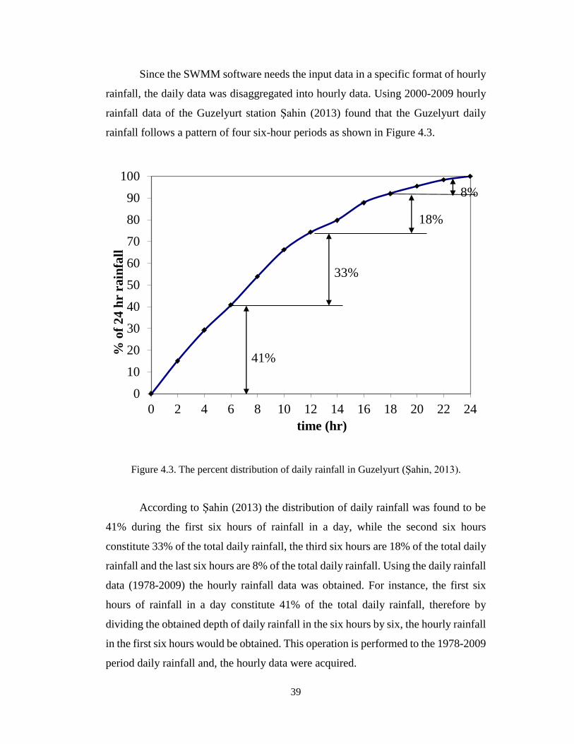
39
Since the SWMM software needs the input data in a specific format of hourly
rainfall, the daily data was disaggregated into hourly data. Using 2000-2009 hourly
rainfall data of the Guzelyurt station Şahin (2013) found that the Guzelyurt daily
rainfall follows a pattern of four six-hour periods as shown in Figure 4.3.
Figure 4.3. The percent distribution of daily rainfall in Guzelyurt (Şahin, 2013).
According to Şahin (2013) the distribution of daily rainfall was found to be
41% during the first six hours of rainfall in a day, while the second six hours
constitute 33% of the total daily rainfall, the third six hours are 18% of the total daily
rainfall and the last six hours are 8% of the total daily rainfall. Using the daily rainfall
data (1978-2009) the hourly rainfall data was obtained. For instance, the first six
hours of rainfall in a day constitute 41% of the total daily rainfall, therefore by
dividing the obtained depth of daily rainfall in the six hours by six, the hourly rainfall
in the first six hours would be obtained. This operation is performed to the 1978-2009
period daily rainfall and, the hourly data were acquired.
0
10
20
30
40
50
60
70
80
90
100
0 2 4 6 8 10 12 14 16 18 20 22 24
% o
f 2
4 h
r ra
infa
ll
time (hr)
8%
41%
33%
18%

40
4.2 Catchment Area
In order to compute the amount of runoff that will be obtained on campus, the
catchment characteristics of the campus should be studied. The existing rainwater
drainage system is built to collect the rainwater from the campus from seven areas.
Using the elevation differences and the suspected movement of rainwater runoff into
the drainage system towards the existing discharge outlets, those seven sub-
catchments were drawn. Each sub-catchment contains a separate discharge outlet and
specific surface characteristics. Computing the areas in each sub-catchment was
performed with the aid of a plan of the campus showing the route of the drainage
system, as well as, the software AutoCAD 2011 to outline the areas of the sub-
catchments and Google Earth to view the different surfaces. Moreover, the area of
the different surfaces was found in order to estimate the runoff. The sub-catchments
can be seen in Figure 4.4.
The seven sub-catchments are as follows:
1. 2nd Lodgment Complex. (Yellow)
2. A-Types Lodgments, B-Types Lodgments, Guest House, EBI Dormitory and
section of the CD-Types Lodgments. (Green)
3. 1st Lodgment Complex, IT Building, Administration Building and section of
the Culture and Convention Center. (Blue)
4. Engineering Laboratories, T-Block, Culture and Convention Center and
section of the School of Foreign Languages Building. (Red)
5. Cafeteria Building, Market Area Buildings (Çarşı), 1st Dormitory, Health
Center Building, S-Block, R-Block, School of Foreign Languages Building
and section of the CD-Types Lodgments. (Purple)
6. Swimming Pool, Sports Complex Building, 2nd Dormitory and 3rd Dormitory.
(Orange)
7. Library (Pink)

41
Sub
-cat
chm
ent
1
Sub
-cat
chm
ent
2
Sub
-cat
chm
ent
3
Sub
-cat
chm
ent
4
Sub
-cat
chm
ent
5
Sub
-cat
chm
ent
6
Sub
-cat
chm
ent
7
Fig
ure
4.4
. P
lan o
f M
ET
U-N
CC
wit
h d
iffe
rent
sub
-cat
chm
ents
colo
red
.

42
4.3 Traditional SCS Method
From the methods discussed previously, one of the runoff methods should be
chosen according to the available parameters and the suitability of the method.
Moreover, the other methods require data that is not available or parameters that need
long experimental work to be determined before applying the method. Since the Soil
Conservation Service (SCS) method includes all types of abstractions in the runoff
calculation and the parameters needed to compute the runoff are available, it is the
most suitable method for this case.
The curve number (CN) of the surface is dependent on the hydrologic soil
group in the study area which is classified according to Table 2.1, the CN of the
surfaces present in sub-catchments can be established using Table 2.2. The
hydrologic soil group of the soil present in the campus region is closest to soil group
D. The description in Table 2.1 defines the type of surface present in the region of
study. Moreover, looking at Table 2.2 one can deduce that the CN of impervious
areas with soil group D is 98 while grass areas with up to 75% grass cover is 84 and
areas with more than 75% grass cover is 80. On the other hand, the CN of open areas
with less than 50% grass cover such as natural forest areas on campus is 89. The
greater the CN, the more the runoff produced by the surface, in other words, the
impervious areas have the greatest runoff potential.
After the CN of each surface is determined, a normalized CN of the sub-
catchment as a whole should be determined by multiplying each specific area with
its corresponding CN, summing the result and dividing that by the total area of the
sub-catchment.
𝐶𝑁𝑁 = ∑ (𝐴𝑖∗𝐶𝑁𝑖
𝐴𝑇)𝑛
𝑖=1 (4.1)
where, 𝐶𝑁𝑁 is the normalized CN of a sub-catchment; 𝐴𝑖 is the area of each surface
in a sub-catchment (m2); 𝐶𝑁𝑖 is the CN of each surface in the sub-catchment; 𝐴𝑇 is
the total area of the sub-catchment (m2); n is the total number of surfaces in the sub-
catchment.

43
After finding “𝐶𝑁𝑁”, the soil moisture deficit is needed to found using the Equation
4.2 (Akan and Houghtalen, 2003),
𝑆𝐷 =25400−254𝐶𝑁𝑁
𝐶𝑁𝑁 (4.2)
where, 𝑆𝐷 is the soil moisture deficit at the time of runoff (mm); 𝐶𝑁𝑁 is the
normalized runoff curve number.
The initial abstraction consisting of the water intercepted by vegetation,
retained in the surface depressions, evaporated or infiltrated before the runoff begins
is calculated by Equation 4.3. Moreover, this equation can only be used if the
precipitation is greater than the initial abstraction (Akan and Houghtalen, 2003),
𝐼𝑎 = 0.2𝑆𝐷 (4.3)
where, 𝐼𝑎 is the initial abstraction (mm); 𝑆𝐷 is the soil moisture deficit at the time of
runoff (mm).
Finally all after those parameters are computed the SCS runoff expression
shown in Equation 4.4 can be employed to compute the runoff (Akan and
Houghtalen, 2003).
𝑅 =(𝑃−𝐼𝑎)2
(𝑃−𝐼𝑎)+𝑆𝐷 (4.4)
where, 𝑅 is the rainfall runoff (mm); 𝑃 is the precipitation (mm); 𝐼𝑎 is the initial
abstraction (mm); 𝑆𝐷 is the soil moisture deficit at the time of runoff (mm).
After the runoff is calculated, the volume of the runoff from each sub-
catchment is computed using Equation 4.5.
𝑉 = 𝑅 ∗ 𝐴𝑇 (4.5)
where, 𝑉 is the volume of runoff (m3); 𝑅 is the rainfall runoff (m); 𝐴𝑇 is the area of
the sub-catchment (m2).

44
4.4 SWMM Model
The Environmental Protection Agency (EPA) developed the Storm Water
Management Model (SWMM), which is a software that is capable of presenting a
dynamic rainfall-runoff simulation model for single storm event simulation or
continuous simulation of runoff quantity and quality from mainly urban sub-
catchment areas (Rossman, 2010). SWMM generates runoff and pollutant
concentrations by operating on a group of sub-catchment areas that receive
precipitation. There is a routing section in SWMM capable of simulating the transport
of this runoff through pipes, channels, storage or treatment devices, pumps and
regulators (Rossman, 2010). Moreover, SWMM is able to track the quantity and
quality of runoff produced in each sub-catchment, the flow rate, the flow depth in
each pipe and channel during a simulation period. SWMM is widely used for
planning, analysis and design of storm-water runoff, sewers and other drainage
systems in urban areas.
SWMM 5.1 provides an integrated environment for controlling study area
input data as well as running hydrologic, hydraulic and water quality simulations.
Furthermore, SWMM allows to view the results in many different formats. SWMM
accounts for various hydrologic processes that contribute to runoff in urban areas,
such as, time- fluctuating rainfall, evaporation, snow accumulation and melting and
infiltration (Rossman, 2010). Dividing the study area into smaller sub-catchment
zones, each exhibiting different characteristics will lead to spatial variability in these
processes. Moreover, this software possesses a collection of hydraulic modeling
options that may be utilized to route runoff and external inflows through the transport
systems. In addition, SWMM can also estimate the accumulation of pollutant loads
related to the runoff. SWMM has ample applications which include designing and
sizing of drainage system components for flood control, sizing of detention facilities
and their accessories for flood control and water quality protection, flood mapping of
natural channel systems and evaluating the effect of inflow and infiltration on sewer
overflows (Rossman, 2010).

45
This software works by creating a conceptual drainage system where water
and pollutants flow through different environmental sections. SWMM has
characterized these sections into various objects in the following form (Rossman,
2010):
The Atmosphere, where the precipitation input data is inserted using the falls
Rain Gage object.
The Land Surface, where the different components and parameters of the
basin area is inserted in the Sub-catchment object. It receives precipitation
from the Atmospheric section and outflow is simulated in the form of
infiltration and surface runoff.
The Groundwater section receives the infiltration output from the previous
section and transfers a part of it to the Transport section. The Aquifer object
is used to model this compartment.
The Transport subdivision, contains a network of transport elements such as
channels, pipes, pumps, and regulators, as well as, storage and treatment units
that carry water to outfalls. The input of this section may come from surface
runoff, groundwater interflow, or from user-defined hydrographs. The Node
and Link objects are used to model the components of this section.
Infiltration of rainfall in a sub-catchment into the unsaturated top soil zone
can be modelled using three different methods (Rossman, 2010):
Horton infiltration
Green-Ampt infiltration
SCS Curve Number infiltration
Moreover, in order to model snow melting or accumulation, the Snow Pack
object should be used, while modelling pollutant accumulation and wash-off the Land
Uses should be managed. Some other important input parameters that are used in the
Sub-catchment object include the appointed rain gage, the outlet node, the land uses,
the imperviousness layer fraction, the sub-catchment slope, the width of overland
flow, the Manning's n for both the pervious and impervious areas and the depression
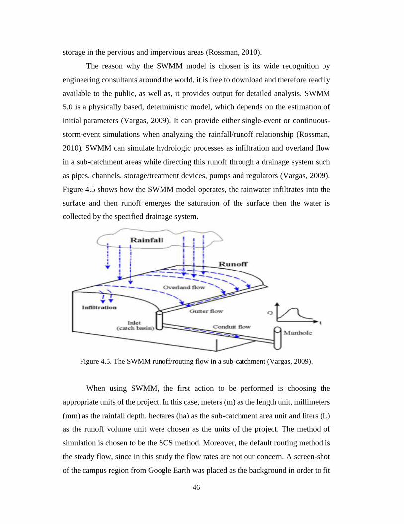
46
storage in the pervious and impervious areas (Rossman, 2010).
The reason why the SWMM model is chosen is its wide recognition by
engineering consultants around the world, it is free to download and therefore readily
available to the public, as well as, it provides output for detailed analysis. SWMM
5.0 is a physically based, deterministic model, which depends on the estimation of
initial parameters (Vargas, 2009). It can provide either single-event or continuous-
storm-event simulations when analyzing the rainfall/runoff relationship (Rossman,
2010). SWMM can simulate hydrologic processes as infiltration and overland flow
in a sub-catchment areas while directing this runoff through a drainage system such
as pipes, channels, storage/treatment devices, pumps and regulators (Vargas, 2009).
Figure 4.5 shows how the SWMM model operates, the rainwater infiltrates into the
surface and then runoff emerges the saturation of the surface then the water is
collected by the specified drainage system.
Figure 4.5. The SWMM runoff/routing flow in a sub-catchment (Vargas, 2009).
When using SWMM, the first action to be performed is choosing the
appropriate units of the project. In this case, meters (m) as the length unit, millimeters
(mm) as the rainfall depth, hectares (ha) as the sub-catchment area unit and liters (L)
as the runoff volume unit were chosen as the units of the project. The method of
simulation is chosen to be the SCS method. Moreover, the default routing method is
the steady flow, since in this study the flow rates are not our concern. A screen-shot
of the campus region from Google Earth was placed as the background in order to fit
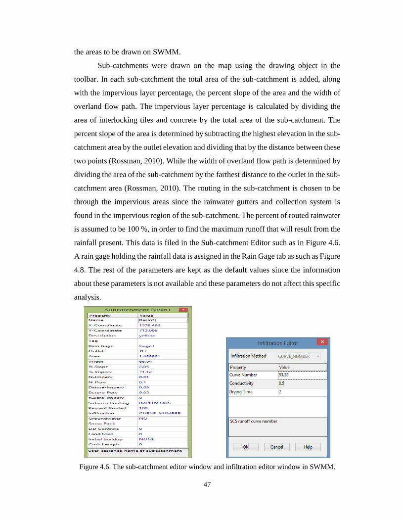
47
the areas to be drawn on SWMM.
Sub-catchments were drawn on the map using the drawing object in the
toolbar. In each sub-catchment the total area of the sub-catchment is added, along
with the impervious layer percentage, the percent slope of the area and the width of
overland flow path. The impervious layer percentage is calculated by dividing the
area of interlocking tiles and concrete by the total area of the sub-catchment. The
percent slope of the area is determined by subtracting the highest elevation in the sub-
catchment area by the outlet elevation and dividing that by the distance between these
two points (Rossman, 2010). While the width of overland flow path is determined by
dividing the area of the sub-catchment by the farthest distance to the outlet in the sub-
catchment area (Rossman, 2010). The routing in the sub-catchment is chosen to be
through the impervious areas since the rainwater gutters and collection system is
found in the impervious region of the sub-catchment. The percent of routed rainwater
is assumed to be 100 %, in order to find the maximum runoff that will result from the
rainfall present. This data is filed in the Sub-catchment Editor such as in Figure 4.6.
A rain gage holding the rainfall data is assigned in the Rain Gage tab as such as Figure
4.8. The rest of the parameters are kept as the default values since the information
about these parameters is not available and these parameters do not affect this specific
analysis.
Figure 4.6. The sub-catchment editor window and infiltration editor window in SWMM.

48
In the Infiltration Editor window the normalized CN is entered, as well as the
soil drying time which has a range from 2 to 14 days. The hydraulic conductivity is
not considered and its value is ignored in this method. The previous is done for each
sub-catchment.
Moreover, an outfall for each sub-catchment is added on the map, from the
Node object under the Hydraulic tab, corresponding to the outlet present in reality. In
addition, a junction is created between each sub-catchment and its respective outfall,
this is done to keep space for the combination of the outlets of different sub-
catchments. The tag or name of each junction is added in the Outlet tab in the sub-
catchment editor of the respective sub-catchment as shown in Figure 4.6. The
junction is connected to the outfall by a conduit or pipe and this added from the Link
tab. When adding the junction and outfall one must make sure that the elevation of
the outfall is lower than that of the junction which is in turn lower than that of the
lowest point in the sub-catchment, in order for the rainwater to flow in the direction
of the outfall. The exact elevations are not necessary since we are not concerned with
the flow rates, the only concern in this study is the volume of outflow. Figure 4.7
shows the junction, conduit and outfall editor windows.
Furthermore, a legend showing the different areas of the sub-catchments can
be added from the Map tab on the left on the window. The next step is to add the
rainfall data, the rain gage tab is used to add the data. The hourly rainfall data is added
in a specific format either in the table present in the Time Series tab or uploaded as
an external file in the same window. The model finally should appear as Figure 4.9.
Before simulating the data, the dates to be simulated should be chosen, in other
words, the start and end of the desired simulation dates should be selected from the
Dates tab under the Options tab; Figure 4.10 shows the simulation dates window.

49
Figure 4.7. The junction, conduit and outfall editor windows on SWMM respectively.
Figure 4.8. The rain gage and time series editor and the rainfall data format.

50
Figure 4.9. The appearance of the SWMM model.
Figure 4.10. The simulation dates options window.

51
4.5 Irrigation Demand
After the runoff volumes of the sub-catchments are computed, the tank
volumes and locations along with the rainwater harvesting system as a whole can be
discussed. The first step is to determine the consumption of water in the sub-
catchments and decide how to distribute the water tanks in order to meet the irrigation
demand in the seven sub-catchments. The vegetation on campus which needs
irrigation was divided into three groups, as ground cover, trees and bushes, and lawn
area. Figure 4.11 shows the three groups of vegetation. The amount of water supplied
to each group of vegetation and the map, shown in Figure 4.12, showing all the
vegetation on the campus was provided by the Directorate of Administrative Affairs
at the METU-NCC in Table 4.1. In order to find the water consumed in each sub-
catchment, the areas of each vegetation group in each sub-catchment are calculated
using the map.
A. B.
C.
Figure 4.11. The three groups of vegetation on campus.
A. Ground cover. B. Trees and bushes. C. Lawn area.

52
Table 4.1. The crop type along with the irrigation requirements.
Crop Type Months of
Irrigation
Duration
(months)
Irrigation
Period
(day/week)
Required
Water per
m2
(L/day)
Total
Water per
m2
(L/month)
Ground
Cover Jan-Dec 12 2 0.87 6.96
Trees and
Bushes Jan-Dec 12 1 20 80
Lawn
Area May-Oct 6 6 12 288
Lawn
Area Nov-Apr 6 5 10 200
Fruit
Trees Mar-Oct 8 3 1.88 22.6

53
Fig
ure
4.1
2. T
he
Auto
CA
D m
ap s
how
ing t
he
veg
etat
ion o
n t
he
cam
pu
s.

54
4.6 Location of Reservoirs
Deciding the location and the number of water reservoirs, as well as the areas
to be irrigated by those reservoirs will be the last step before calculating the volumes
of the water tanks. Since the collection of water is occurring at the lowest elevations
of the campus then pumping is a necessity. Since constructing seven water tanks will
be costly, combining the runoff from different sub-catchments and storing it in the
same reservoir may be a better option keeping in consideration the areas to be
irrigated. Many alternatives may be proposed, one option that will be discussed and
assessed for the reliability is as shown in Figure 4.10. This option will be discussed
to show that the system has the potential to operate and produce adequate results. The
runoff of Sub-catchments 1, 2 and 7 can be combined in one tank and stored in
Position 1 on the map, while the runoff from sub-catchments 3 and 4 can be combined
into Position 2 and the runoff from Sub-catchments 5 and 6 can be stored in Position
3 as shown on the map.
Using this combination of reservoirs the areas to be irrigated will be Sub-
catchments 1, 2, 6 and the top part of Sub-catchment 5 from the reservoir at Position
1, while the reservoir at Position 2 will be used to irrigate Sub-catchments 3, 4, 7 and
the lower part of Sub-catchment 5, on the other hand, the reservoir at Position 3 will
irrigate the tree fruits at the bottom of the campus, outlined in green in Figure 4.13
and presented in Table 4.2. The blue spots on the map stand for small plastic tanks
that act as temporary storage before the water is used by the irrigation system.
Table 4.2. The reservoirs, the sub-catchments supplying their runoff and the corresponding
irrigation areas.
Reservoir Runoff from Sub-catchments Sub-catchments to be irrigated
Reservoir 1 Sub-catchments 1, 2 and 7 Sub-catchments 1, 2, 6 and top part of 5
Reservoir 2 Sub-catchments 3, 4 Sub-catchments 3, 4, 7 and lower part of 5
Reservoir 3 Sub-catchments 5, 6 Fruit trees

55
Figu
re 4
.13
. Th
e m
ap w
ith
res
erv
oir
loca
tio
ns
and
irri
gati
on
are
as o
n c
amp
us.

56
Fig
ure 4
.14. T
he area th
at Reserv
oir 1
irrigates.
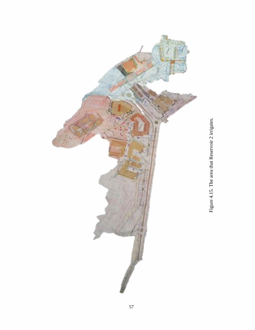
57
Fig
ure
4.1
5. T
he
area
that
Res
ervoir
2 i
rrig
ates
.

58
4.6 Tank Size Calculation Method
Accordingly, the monthly water consumption for each sub-catchment can be
computed and will be used to calculate the reservoir volumes. In order to perform such a
task a water balance approach should be adopted, showing the water demand met from the
excess precipitation. The water balance approach is similar to the Simple Tabular Method
described in Chapter II (page 21). Two types of balances will be adopted the annual
balance and the monthly balance. The annual balance will include the carryover of the
excess stored water from one year to the next as well as from one month to the next. While
the monthly balance will not have any carryover from the previous month or year. The
monthly runoff is computed from the monthly simulations of SWMM. The tank volume
will be computed using the method given in Nnaji and Mama (2014). In this method the
Storage Capacity (SC), is calculated by subtracting the cumulative surplus at the end of
the year from the maximum cumulative surplus. The Cumulative Surplus (CS) is computed
using Equation 4.6, moreover, if the inflow and the water stored from the previous month
is less than the demand then a deficit occurs and a value of zero is assigned (Nnaji and
Mama, 2014). When calculating the volumes of the tanks in each year, water years will be
considered not the regular year will be studied, for instance 1978-1979 will start at
September 1978 and end at August 1979.
𝐶𝑆𝑖 = {0, (𝑖𝑓 𝐶𝑆𝑖−1 + 𝑅𝑖 − 𝐷𝑖 ≤ 0) 𝑒𝑙𝑠𝑒
𝐶𝑆𝑖−1 + 𝑅𝑖 − 𝐷𝑖 (4.6)
where 𝐶𝑆𝑖 is the cumulative surplus of the current month; 𝐶𝑆𝑖−1 is the cumulative surplus
of the previous month (m3); 𝑅𝑖 is the runoff of the current month (m3); 𝐷𝑖 is the demand
of the current month (m3).
Equation 4.7 illustrates how to compute the water in storage, if the inflow and the
water in storage from the previous month is less than the demand then there will be no
water to store. If the same expression is greater than or equal to the storage capacity then
the value of the water in the storage is the storage capacity, which is the maximum value
for the water in storage, otherwise the difference between the sum of the inflow and the

59
water storage of the previous month and the demand is the water storage of the current
month (Nnaji and Mama, 2014).
𝑊𝑆𝑖 = {
0, (𝑖𝑓 𝑅𝑖 + 𝑊𝑆𝑖−1 − 𝐷𝑖 < 0) 𝑒𝑙𝑠𝑒
𝑆𝐶, (𝑖𝑓 𝑅𝑖 + 𝑊𝑆𝑖−1 − 𝐷𝑖 ≥ 𝑆𝐶) 𝑒𝑙𝑠𝑒𝑅𝑖 + 𝑊𝑆𝑖−1 − 𝐷𝑖
(4.7)
where 𝑊𝑆𝑖 is the water in storage of the current month; 𝑊𝑆𝑖−1 is the water in storage of
the previous month; 𝑆𝐶 is the storage capacity.
In this study the aim is not to maximize the storage but to investigate if the water
demand can be satisfied through the rainfall, therefore, excess water during a month may
be spilled. Equation 4.8 shows how the spillage of the annual balance may be computed.
There will be no spillage if the water in storage of the current month is less than the storage
capacity else the spillage is the difference between the water storage of the current month
and the storage capacity (Nnaji and Mama, 2014).
𝑆𝑃1𝑖 = {0, (𝑖𝑓 𝑅𝑖 + 𝑊𝑆𝑖−1 − 𝐷𝑖 < 𝑆𝐶) 𝑒𝑙𝑠𝑒
𝑅𝑖 + 𝑊𝑆𝑖−1 − 𝐷𝑖 − 𝑆𝐶 (4.8)
where 𝑆𝑃1𝑖 is the water in storage of the current month in the annual balance.
To compute the demand met for each month in the annual balance Equation 4.9 is
used. If the water in storage of the current month is greater than or equal to zero then the
demand met is the demand of the current month otherwise the demand met is the sum of
the inflow of the current month and the water in storage of the previous month (Nnaji and
Mama, 2014).
𝐷𝑀1𝑖 = {𝐷𝑖, (𝑖𝑓 𝑅𝑖 + 𝑊𝑆𝑖−1 − 𝐷𝑖 ≥ 0) 𝑒𝑙𝑠𝑒
𝑅𝑖 + 𝑊𝑆𝑖−1 (4.9)
where 𝐷𝑀1𝑖 is the demand met of the current month in the annual balance.

60
Moreover, in turn the monthly rainfall was assessed to identify the sufficiency to
satisfy the monthly demand without utilizing water from the previous month. If the
difference between the inflow and demand in one month is greater than zero then the
demand met is equal to the demand of that month, otherwise the demand met is the inflow
of the current month. When the demand in a month is met, the remaining surplus is spilled,
otherwise there will be no spill (Nnaji and Mama, 2014). Equation 4.10 and 4.11 show the
demand met and spillage expressions respectively in the monthly balance approach.
𝐷𝑀2𝑖 = {𝐷𝑖, (𝑖𝑓 𝑅𝑖 − 𝐷𝑖 > 0) 𝑒𝑙𝑠𝑒
𝑅𝑖 (4.10)
where 𝐷𝑀2𝑖 is the demand met of the current month in the monthly balance.
𝑆𝑃2𝑖 = {𝑅𝑖 − 𝐷𝑀𝑖, (𝑖𝑓 𝑅𝑖 − 𝐷𝑀𝑖 > 0) 𝑒𝑙𝑠𝑒
0 (4.11)
where 𝑆𝑃2𝑖 is the spillage of the current month in the monthly balance.

61
CHAPTER V
CALCULATIONS, RESULTS AND DISCUSSION
5.1 Catchment Area
Using Figure 4.4 and Google Earth, the areas of each surface in the seven sub-
catchments were determined as shown in Table 5.1. It can be inferred that the artificial
compacted sand surface is only found in sub-catchments 3 and 6, and that the rubber
surface is only present in sub-catchment 6 while sub-catchments 4 and 5 are the only sub-
catchments that contain natural environment areas. Since gutters are not found in some
areas of the campus, not all the area is covered by the rainwater drainage system. The total
campus area that rainwater will be collected from is 346,971 m2.
Table 5.1. Areas (m2) of every surface in each sub-catchment
Sub-
catchment
Interlocking
Tiles and
Concrete
Area
Grass
Area
Artificial
sand Area
Rubber
Area
Natural
Environment
Area
Total
Area
1 10589 4299 0 20 0 14888
2 28834 15857 0 0 0 44691
3 21376 12604 589 0 0 34569
4 31646 9685 0 0 7029 48360
5 72100 20232 0 0 32130 124462
6 40397 25631 1311 5690 0 73029
7 5732 1239 0 0 0 6971
Total 210675 89547 1900 5690 39159 346971
5.2 Catchment Runoff
After the areas of the surfaces on campus are determined the parameters needed in
the runoff calculation need to be computed. For the traditional SCS method parameters
such as 𝑆𝐷, 𝐼𝑎 and 𝐶𝑁𝑁 are required in the runoff calculation. On the other hand, in the
SWMM model parameters such as the percent of impervious layer, percent slope and the
width of overflow need to be determined before applying the model.

62
5.2.1 Traditional SCS Results
When applying this method the CN of each surface is determined from Table 2.2
according to soil group D. 𝐶𝑁𝑁 is determined from Equation 4.1, while 𝑆𝐷 is computed
from Equation 4.2 and 𝐼𝑎 is computed from Equation 4.3. The data is placed into a table
similar to Table 5.2, to calculate the monthly runoff produced by each sub-catchment.
Table 5.2. The data used in the spreadsheet SCS method.
Sub-Catchment
Surface Type
1 2 3 4 5 6 7
Interlocking Tiles
and Concrete Area
(m2)
10589 28834 21376 31646 72100 40397 5732
CN 98 98 98 98 98 98 98
Grass Area (m2) 4299 15857 12604 9685 20232 25631 1239
CN 82 82 82 82 82 82 82
Artificial sand Area
(m2) 0 0 589 0 0 1311 0
CN 88 88 88 88 88 88 88
Rubber Area (m2) 0 0 0 0 0 5690 0
CN 98 98 98 98 98 98 98
Natural
Environment Area
(m2)
0 0 0 7029 32130 0 0
CN 89 89 89 89 89 89 89
Total Area (m2) 14888 44691 34569 48360 124462 73029 6971
CNN 93.38 92.32 92.00 93.49 93.08 92.20 95.16
SD (mm) 18.00 21.12 23.38 17.69 18.90 22.82 12.93
Ia (mm) 3.60 4.22 4.68 3.54 3.78 4.56 2.59
After the individual monthly precipitation values are plugged into the spreadsheet
from 1978 to 2009, the monthly runoff volumes of each sub-catchment will be obtained
by using Equation 4.4. The results showed that the 5th sub-catchment will obtain the largest
runoff volume while the 7th sub-catchment will have the least runoff volume, this is mainly

63
due to the difference in the areas of the sub-catchments, although the 7th sub-catchment
has the highest percent of impervious layer. Table 5.3 shows the results of runoff in 1978
according to the traditional SCS method.
Table 5.3. Spreadsheet monthly runoff volume (m3) from each sub-catchment.
1978 Jan Feb Mar Apr May Jun Jul Aug Sep Oct Nov Dec
Rainfall 104.7 27.5 56.2 25.3 0.0 0.0 0.0 0.0 0.0 29.0 8.0 91.1
Sub-
catchment 1 1277.6 202.9 583.4 176.5 0.0 0.0 0.0 0.0 0.0 221.3 12.9 1080.4
Sub-
catchment 2 3710.4 545.4 1651.7 470.4 0.0 0.0 0.0 0.0 0.0 597.7 25.6 3123.2
Sub-
catchment 3 2802.6 389.7 1225.1 334.1 0.0 0.0 0.0 0.0 0.0 428.7 14.3 2351.4
Sub-
catchment 4 4163.9 666.6 1906.2 580.4 0.0 0.0 0.0 0.0 0.0 726.5 43.4 3522.6
Sub-
catchment 5 10579.9 1643.3 4795.7 1426.2 0.0 0.0 0.0 0.0 0.0 1794.5 95.9 8934.7
Sub-
catchment 6 5955.6 839.6 2615.2 720.9 0.0 0.0 0.0 0.0 0.0 922.8 32.8 5000.9
Sub-
catchment 7 631.8 114.3 301.1 100.9 0.0 0.0 0.0 0.0 0.0 123.6 11.1 538.4
5.2.2 SWMM Model Results
In order to apply the SWMM software to compute the runoff the percent
impervious layer, width of overflow and the percent slope are calculated and the results of
these calculations are shown in Table 5.4. These parameters are placed in the input of the
SWMM software in the sub-catchment characteristics. Since the SWMM model requires
hourly rainfall, the daily rainfall data was converted to hourly rainfall using Figure 4.3.
Some of the hourly rainfall are presented in Table 5.6 and are calculated from the daily
rainfall in Table 5.5. Table 5.7 shows the SWMM monthly runoff in 1978.

64
Table 5.4. The input data in the SWMM model for all the sub-catchments.
Sub-Catchment 1 2 3 4 5 6 7
Total Area (ha) 1.4888 4.4691 3.4569 4.836 12.4462 7.3029 0.6971
CNN 93.38 92.32 92.00 93.49 93.08 92.20 95.16
Interlocking
Tiles and
Concrete Area
(ha)
1.0589 2.8834 2.1376 3.1646 7.2100 4.0397 0.5732
Percent of
Impervious
Layer (%)
71.12 64.52 63.54 65.44 57.93 64.90 82.22
Length from
outlet to
farthest point
(m)
225.44 845.14 446.22 282.39 1340.32 847.90 139.31
Width of
overflow(m) 66.04 52.88 77.47 171.25 92.86 86.13 50.04
Highest
Elevation (m) 142.5 143.9 139.6 132 140.1 142 135.9
Lowest
Elevation (m) 137.4 133.3 131.1 118.2 92 115.2 132.4
Distance
between highest
and lowest
points (m)
248.7 775.1 518.3 219.2 1286.4 770.5 150
Percent slope
(%) 2.05 1.37 1.64 6.30 3.74 3.48 2.33
Drying time
(days) 8 8 8 8 8 8 8
Table 5.5. Daily rainfall data (mm) of days 1 to 10 in each month of 1978
Day Jan Feb Mar Apr May Jun Jul Aug Sep Oct Nov Dec
1 0.0 0.0 0.0 0.0 0.0 0.0 0.0 0.0 0.0 0.0 0.0 0.0
2 1.3 0.0 0.0 0.0 0.0 0.0 0.0 0.0 0.0 0.0 0.0 0.0
3 28.7 2.8 0.0 0.0 0.0 0.0 0.0 0.0 0.0 0.0 0.0 0.0
4 2.1 1.3 0.0 0.0 0.0 0.0 0.0 0.0 0.0 0.0 0.0 21.5
5 0.0 0.0 0.0 0.0 0.0 0.0 0.0 0.0 0.0 0.0 0.0 0.0
6 0.0 0.0 0.8 0.0 0.0 0.0 0.0 0.0 0.0 0.0 5.5 21.5
7 0.0 2.2 0.0 0.0 0.0 0.0 0.0 0.0 0.0 0.0 2.5 4.2
8 2.2 1.2 0.0 0.0 0.0 0.0 0.0 0.0 0.0 0.0 0.0 1.9
9 0.8 0.6 0.0 0.0 0.0 0.0 0.0 0.0 0.0 0.0 0.0 0.0
10 23.1 0.5 0.0 0.0 0.0 0.0 0.0 0.0 0.0 0.0 0.0 9.6
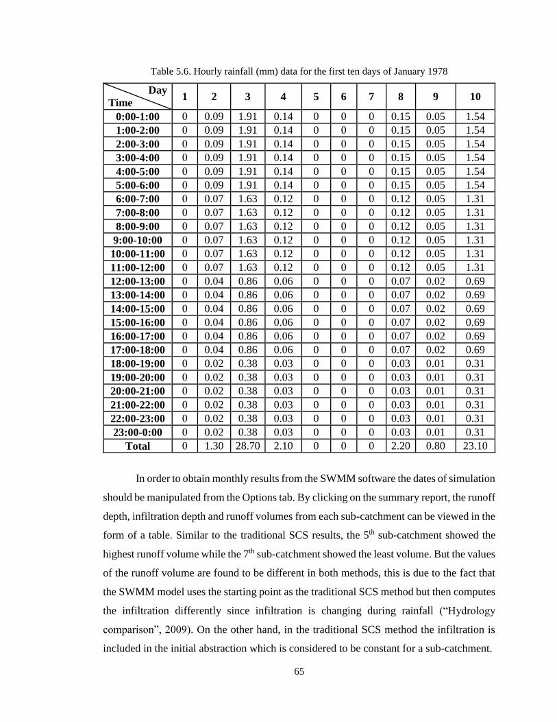
65
Table 5.6. Hourly rainfall (mm) data for the first ten days of January 1978
Day
Time 1 2 3 4 5 6 7 8 9 10
0:00-1:00 0 0.09 1.91 0.14 0 0 0 0.15 0.05 1.54
1:00-2:00 0 0.09 1.91 0.14 0 0 0 0.15 0.05 1.54
2:00-3:00 0 0.09 1.91 0.14 0 0 0 0.15 0.05 1.54
3:00-4:00 0 0.09 1.91 0.14 0 0 0 0.15 0.05 1.54
4:00-5:00 0 0.09 1.91 0.14 0 0 0 0.15 0.05 1.54
5:00-6:00 0 0.09 1.91 0.14 0 0 0 0.15 0.05 1.54
6:00-7:00 0 0.07 1.63 0.12 0 0 0 0.12 0.05 1.31
7:00-8:00 0 0.07 1.63 0.12 0 0 0 0.12 0.05 1.31
8:00-9:00 0 0.07 1.63 0.12 0 0 0 0.12 0.05 1.31
9:00-10:00 0 0.07 1.63 0.12 0 0 0 0.12 0.05 1.31
10:00-11:00 0 0.07 1.63 0.12 0 0 0 0.12 0.05 1.31
11:00-12:00 0 0.07 1.63 0.12 0 0 0 0.12 0.05 1.31
12:00-13:00 0 0.04 0.86 0.06 0 0 0 0.07 0.02 0.69
13:00-14:00 0 0.04 0.86 0.06 0 0 0 0.07 0.02 0.69
14:00-15:00 0 0.04 0.86 0.06 0 0 0 0.07 0.02 0.69
15:00-16:00 0 0.04 0.86 0.06 0 0 0 0.07 0.02 0.69
16:00-17:00 0 0.04 0.86 0.06 0 0 0 0.07 0.02 0.69
17:00-18:00 0 0.04 0.86 0.06 0 0 0 0.07 0.02 0.69
18:00-19:00 0 0.02 0.38 0.03 0 0 0 0.03 0.01 0.31
19:00-20:00 0 0.02 0.38 0.03 0 0 0 0.03 0.01 0.31
20:00-21:00 0 0.02 0.38 0.03 0 0 0 0.03 0.01 0.31
21:00-22:00 0 0.02 0.38 0.03 0 0 0 0.03 0.01 0.31
22:00-23:00 0 0.02 0.38 0.03 0 0 0 0.03 0.01 0.31
23:00-0:00 0 0.02 0.38 0.03 0 0 0 0.03 0.01 0.31
Total 0 1.30 28.70 2.10 0 0 0 2.20 0.80 23.10
In order to obtain monthly results from the SWMM software the dates of simulation
should be manipulated from the Options tab. By clicking on the summary report, the runoff
depth, infiltration depth and runoff volumes from each sub-catchment can be viewed in the
form of a table. Similar to the traditional SCS results, the 5th sub-catchment showed the
highest runoff volume while the 7th sub-catchment showed the least volume. But the values
of the runoff volume are found to be different in both methods, this is due to the fact that
the SWMM model uses the starting point as the traditional SCS method but then computes
the infiltration differently since infiltration is changing during rainfall (“Hydrology
comparison”, 2009). On the other hand, in the traditional SCS method the infiltration is
included in the initial abstraction which is considered to be constant for a sub-catchment.

66
Table 5.7. SWMM monthly runoff volume (m3) from each sub-catchment.
1978 Jan Feb Mar Apr May Jun Jul Aug Sep Oct Nov Dec
Rainfall 104.7 27.5 56.2 25.3 0.0 0.0 0.0 0.0 0.0 29.0 8.0 91.1
Sub-
catchment 1 1402 330 716 330 0 0 0 0 0 362 95 1213
Sub-
catchment 2 4023 916 2028 944 0 0 0 0 0 1002 265 3473
Sub-
catchment 3 3031 682 1523 711 0 0 0 0 0 761 197 2615
Sub-
catchment 4 4465 1021 2252 1045 0 0 0 0 0 1137 294 3853
Sub-
catchment 5 11053 2426 5476 2570 0 0 0 0 0 2673 699 9515
Sub-
catchment 6 6464 1463 3254 1518 0 0 0 0 0 1606 423 5581
Sub-
catchment 7 696 172 363 165 0 0 0 0 0 185 50 604
5.2.3 Sensitivity Analysis
The difference between the two approaches is that the SWMM model uses CN to
compute the infiltration as a starting point and then SWMM utilizes the runoff
methodology to simulate the surface runoff hydrograph as stated by Lewis A. Rossman,
the author of the SWMM user manual (Rossman, 2009). Some parameters included in the
SWMM model but not in the spreadsheet SCS are the percent of impervious layer,
depression storage, the pervious roughness coefficient and the soil drying time. The exact
value of the soil drying time parameter can be determined through experimental analysis
and the information regarding this parameter is not available, therefore a sensitivity
analysis is performed to assess the effect of this parameter on the runoff. The range of this
parameter on SWMM is between 2 days and 14 days.
The sensitivity analysis was performed on the two years with the highest annual
precipitation which were 1988 and 1994 with 470.1 mm and 484.8 mm respectively. The
monthly runoff was found for different values of the saturated soil drying time. The
saturated soil drying time ranges from 2 days to 14 days with a median of 8 days. Figures
5.1 to 5.7 show the sensitivity of each sub-catchment to changing the saturated soil drying
time. In Figures 5.1 to 5.7 the curves of April to October appear as one curve since during
these months there is no or little rainfall so the change in the runoff due to the change in
the saturated soil drying time is negligible. Moreover, the highest monthly rainfall through
all the data such as 2003 February, 2010 January and 1986 November, with 159 mm, 154.7

67
mm and 131.2 mm respectively, were analyzed individually with respect to changing
saturated soil drying time. In this analysis a major effect is indicated when the parameter
was varied and the runoff change is greater than ± 5%, as shown in Figure 5.8. Both
sensitivity tests illustrated the runoff is not sensitive to the change in soil saturated drying
time. The main reason for the runoff not being sensitive to the change in the soil saturated
drying time is that the sub-catchment areas are mainly consisting of impervious layers as
seen from Table 5.4 the percent of impervious layer range from 57.9% to 71.1%, therefore,
there is little effect on the runoff from the soil surface.
Figure 5.1. The effect of change in saturated soil drying time on runoff in sub-catchment 1.
-3.5
-3
-2.5
-2
-1.5
-1
-0.5
0
0.5
1
1.5
2
0 2 4 6 8 10 12 14 16
Per
cen
t ch
ange
of
sub
-cat
chm
ent
run
off
Saturated soil drying time period (days)
Sub-catchment 1
Jan
Feb
Mar
Apr
May
Jun
Jul
Aug
Sep
Oct
Nov
Dec
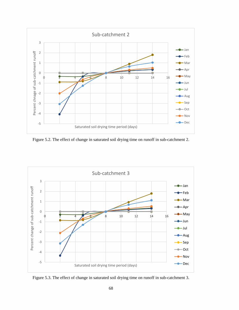
68
Figure 5.2. The effect of change in saturated soil drying time on runoff in sub-catchment 2.
Figure 5.3. The effect of change in saturated soil drying time on runoff in sub-catchment 3.
-5
-4
-3
-2
-1
0
1
2
3
0 2 4 6 8 10 12 14 16
Per
cen
t ch
nag
e o
f su
b-c
atch
men
t ru
no
ff
Saturated soil drying time period (days)
Sub-catchment 2
Jan
Feb
Mar
Apr
May
Jun
Jul
Aug
Sep
Oct
Nov
Dec
-5
-4
-3
-2
-1
0
1
2
3
0 2 4 6 8 10 12 14 16
Per
cen
t ch
ange
of
sub
-cat
chm
ent
run
off
Saturated soil drying time period (days)
Sub-catchment 3
Jan
Feb
Mar
Apr
May
Jun
Jul
Aug
Sep
Oct
Nov
Dec

69
Figure 5.4. The effect of change in saturated soil drying time on runoff in sub-catchment 4.
Figure 5.5. The effect of change in saturated soil drying time on runoff in sub-catchment 5.
-4
-3
-2
-1
0
1
2
3
0 2 4 6 8 10 12 14 16
Per
cen
t ch
ange
of
sub
-cat
chm
ent
run
off
Saturated soil drying time period (days)
Sub-catchment 4
Jan
Feb
Mar
Apr
May
Jun
Jul
Aug
Sep
Oct
Nov
Dec
-5
-4
-3
-2
-1
0
1
2
3
0 2 4 6 8 10 12 14 16
Per
cen
t ch
ange
of
sub
-cat
chm
ent
run
off
Saturated soil drying time period (days)
Sub-catchment 5
Jan
Feb
Mar
Apr
May
Jun
Jul
Aug
Sep
Oct
Nov
Dec

70
Figure 5.6. The effect of change in saturated soil drying time on runoff in sub-catchment 6.
Figure 5.7. The effect of change in saturated soil drying time on runoff in sub-catchment 7.
-5
-4
-3
-2
-1
0
1
2
3
0 2 4 6 8 10 12 14 16
Per
cen
t ch
ange
of
sub
-cat
chm
ent
run
off
Saturated soil drying time period (days)
Sub-catchment 6
Jan
Feb
Mar
Apr
May
Jun
Jul
Aug
Sep
Oct
Nov
Dec
-1.5
-1
-0.5
0
0.5
1
1.5
0 2 4 6 8 10 12 14 16
Per
cen
t ch
ange
of
sub
-cat
chm
ent
run
off
Saturated soil drying time period (days)
Sub-catchment 7
Jan
Feb
Mar
Apr
May
Jun
Jul
Aug
Sep
Dec
Oct
Nov

71
Figure 5.8. The effect of change in saturated soil drying time on runoff in all sub-catchments
during the peak monthly rainfall.
5.3 Irrigation Requirements
The monthly irrigation requirements of each sub-catchment are calculated by
multiplying the monthly water demand of each vegetation type shown in Table 4.2 by the
corresponding areas of the vegetation in each sub-catchment from Table 5.9. Moreover,
Table 5.8 shows that Sub-catchments 1 and 2 do not contain any lawn areas. Due to that
reason, the monthly water consumption of Sub-catchments 1 and 2 are the same throughout
all the months of the year as presented in Table 5.9. Consequently, the monthly demand of
each reservoir should be summed, this is shown in Table 5.10.
-4
-3
-2
-1
0
1
2
0 2 4 6 8 10 12 14 16
Per
cen
t ch
ange
of
sub
-cat
chm
ent
run
off
Saturated soil drying time period (days)
Monthly Peak Rainfall
Sub-catchment 1
Sub-catchment 2
Sub-catchment 3
Sub-catchment 4
Sub-catchment 5
Sub-catchment 6
Sub-catchment 7

72
Table 5.8. The areas occupied of each crop type in the seven sub-catchments.
Sub- catchment Ground cover (m2)
Trees and bushes
Lawn area (m2) m2
Number of
trees and
bushes
Sub-catchment 1 2324 1976 1149 0
Sub- catchment 2 6938 8919 5185 0
Sub- catchment 3 2779 6286 3653 3540
Sub- catchment 4 4714 1876 1091 3095
Sub- catchment 5 5211 1922 1117 13099
Sub- catchment 6 15263 9286 5399 1082
Sub- catchment 7 162 480 279 1259
Total Area 37390 30745 17873 22074
Table 5.9. The monthly water consumption (m3) of each sub-catchment.
Sub-catchment
Month
1 2 3 4 5 6 7
Jan 174 762 1230 802 2810 1065 291
Feb 174 762 1230 802 2810 1065 291
Mar 174 762 1230 802 2810 1065 291
Apr 174 762 1230 802 2810 1065 291
May 174 762 1542 1074 3963 1161 402
Jun 174 762 1542 1074 3963 1161 402
Jul 174 762 1542 1074 3963 1161 402
Aug 174 762 1542 1074 3963 1161 402
Sep 174 762 1542 1074 3963 1161 402
Oct 174 762 1542 1074 3963 1161 402
Nov 174 762 1230 802 2810 1065 291
Dec 174 762 1230 802 2810 1065 291

73
Table 5.10. The monthly water consumption (m3) of the three irrigation areas.
Month Reservoir 1 Reservoir 2 Reservoir 3
Jan 3406 3728 0
Feb 3406 3728 0
Mar 3406 3728 369
Apr 3406 3728 369
May 4078 4999 369
Jun 4078 4999 369
Jul 4078 4999 369
Aug 4078 4999 369
Sep 4078 4999 369
Oct 4078 4999 369
Nov 3406 3728 0
Dec 3406 3728 0
Annual Consumption 44906 52365 2950
Total Annual
Consumption of
campus
100221
5.4 Rainwater Tank Sizing Results
Before calculating the reservoir volumes, the runoff from one of two methods used
should be chosen to be utilized in the reservoir sizing calculations. The traditional SCS
method has some drawbacks when compared to the SWMM model. The traditional SCS
is considered to be a combined loss method since the initial abstraction includes
infiltration, interception and depression storage, the losses caused by these processes are
calculated simultaneously. Moreover, in the traditional SCS method the infiltration in the
initial abstraction does not vary with changing rainfall events on a sub-catchment, on the
contrary it would stay the same before and during the rainfall event. On the other hand, in
the SWMM model, the infiltration changes with changing rainfall events and therefore the
SWMM model simulates infiltration better than the traditional SCS. Therefore, the runoff
results from the SWMM model were chosen to be utilized in the tank sizing calculations.
After applying Equations 4.6 to 4.11, the annual reservoir volume is computed such as in
Table 5.12. The volumes of the three water reservoirs were taken as the average of all the
years without the years that showed zero as the volume of the water tanks. Since rainwater
will not be collected in those years, they will not be included in the reservoir sizing
calculations. Furthermore, Reservoir 1 was computed to be 2305 m3, Reservoir 2 was
calculated as 3490 m3 while Reservoir 3 was computed to be 1071 m3. The percentage of
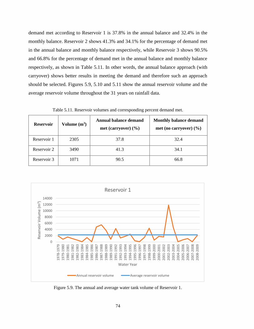
74
demand met according to Reservoir 1 is 37.8% in the annual balance and 32.4% in the
monthly balance. Reservoir 2 shows 41.3% and 34.1% for the percentage of demand met
in the annual balance and monthly balance respectively, while Reservoir 3 shows 90.5%
and 66.8% for the percentage of demand met in the annual balance and monthly balance
respectively, as shown in Table 5.11. In other words, the annual balance approach (with
carryover) shows better results in meeting the demand and therefore such an approach
should be selected. Figures 5.9, 5.10 and 5.11 show the annual reservoir volume and the
average reservoir volume throughout the 31 years on rainfall data.
Table 5.11. Reservoir volumes and corresponding percent demand met.
Reservoir Volume (m3) Annual balance demand
met (carryover) (%)
Monthly balance demand
met (no carryover) (%)
Reservoir 1 2305 37.8 32.4
Reservoir 2 3490 41.3 34.1
Reservoir 3 1071 90.5 66.8
Figure 5.9. The annual and average water tank volume of Reservoir 1.
0
2000
4000
6000
8000
10000
12000
14000
19
78
-19
79
19
79
-19
80
19
80
-19
81
19
81
-19
82
19
82
-19
83
19
83
-19
84
19
84
-19
85
19
85
-19
86
19
86
-19
87
19
87
-19
88
19
88
-19
89
19
89
-19
90
19
91
-19
92
19
92
-19
93
19
93
-19
94
19
94
-19
95
19
95
-19
96
19
96
-19
97
19
97
-19
98
19
98
-19
99
19
99
-20
00
20
00
-20
01
20
01
-20
02
20
02
-20
03
20
03
-20
04
20
04
-20
05
20
05
-20
06
20
06
-20
07
20
07
-20
08
20
08
-20
09
Res
ervo
ir V
olu
me
(m3 )
Water Year
Reservoir 1
Annual reservoir volume Average reservoir volume

75
Au
g
0.0
0
40
78
0
0
0
0
0
0
0
0
4812.5
8
Ju
l
0.0
0
40
78
0
0
0
0
0
0
0
0
Ju
n
1.6
72
40
78
0
0
0
72
72
0
1.8
1.8
Ma
y
2.8
13
1
40
78
0
0
0
13
1
13
1
0
3.2
3.2
Ap
r
2.4
10
1
34
06
.4
0
0
0
21
16
.9
10
1
0
62
.1
3.0
Ma
r
89.3
5311
3406
.4
2015
.9
2015
.9
0
3406
.4
3406
.4
1904
.6
100
100
Feb
17.0
870
3406.4
111.3
111.3
0
3406.4
870
0
100
25.5
Jan
57.8
3192
3406.4
2647.7
2647.7
0
3406.4
3192
0
100
93.7
Dec
26.8
1456
3406.4
2862.2
2862.2
0
3406.4
1456
0
100
42.7
Nov
131.1
8219
3406.4
4812.6
4812.6
0
3406.4
3406.4
4812.6
100
100
Oct
11.6
562
4078
0
0
0
562
562
0
13.8
13.8
Sep
0.2
6
40
78
0
0
0
6
6
0
0.1
5
0.1
5
19
86-1
98
7
Ra
infa
ll (
mm
)
Ru
no
ff (
m3)
Dem
an
d (
m3)
CS
(m
3)
WS
(m
3)
SP
1 (
m3)
DM
1 (
m3)
DM
2 (
m3)
SP
2 (
m3)
%D
M1
%D
M2
SC
(m
3)
Tab
le 5
.12. T
he
wat
er b
alan
ce d
uri
ng 1
986
-1987 t
o f
ind t
he
volu
me
of
Res
ervo
ir 1
.

76
.
Figure 5.10. The annual and average water tank volume of Reservoir 2.
Figure 5.11. The annual and average water tank volume of reservoir 3.
0
2000
4000
6000
8000
10000
12000
14000
16000
19
78
-19
79
19
79
-19
80
19
80
-19
81
19
81
-19
82
19
82
-19
83
19
83
-19
84
19
84
-19
85
19
85
-19
86
19
86
-19
87
19
87
-19
88
19
88
-19
89
19
89
-19
90
19
90
-19
91
19
91
-19
92
19
92
-19
93
19
93
-19
94
19
94
-19
95
19
95
-19
96
19
96
-19
97
19
97
-19
98
19
98
-19
99
19
99
-20
00
20
00
-20
01
20
01
-20
02
20
02
-20
03
20
03
-20
04
20
04
-20
05
20
05
-20
06
20
06
-20
07
20
07
-20
08
20
08
-20
09
Res
ervo
ir v
olu
me
(m3 )
Water Year
Reservoir 2
Annual reservoir volume Average reservoir volume
0
500
1000
1500
2000
19
78
-19
79
19
79
-19
80
19
80
-19
81
19
81
-19
82
19
82
-19
83
19
83
-19
84
19
84
-19
85
19
85
-19
86
19
86
-19
87
19
87
-19
88
19
88
-19
89
19
89
-19
90
19
90
-19
91
19
91
-19
92
19
92
-19
93
19
93
-19
94
19
94
-19
95
19
95
-19
96
19
96
-19
97
19
97
-19
98
19
98
-19
99
19
99
-20
00
20
00
-20
01
20
01
-20
02
20
02
-20
03
20
03
-20
04
20
04
-20
05
20
05
-20
06
20
06
-20
07
20
07
-20
08
20
08
-20
09Res
ervo
ir v
olu
me
(m3)
Water Year
Reservoir 3
Annual Reservoir Volume Average reservoir volume

77
Table 5.13. Annual water demand and annual saving.
Reservoir Annual Water
Demand (m3)
Percent of Water
Demand Met (%)
Annual Water
Demand met (m3)
Reservoir 1 44,906 37.8 16,974
Reservoir 2 52,365 41.3 21,627
Reservoir 3 2,950 90.5 2,670
Total 100,221 41.2 41,271
As shown in Table 5.13 the annual water supplied by the proposed system is 41,271
m3, which is 41.2% of the total annual irrigation demand of the campus. The proposed
system can be integrated with the present irrigation system by pumping the water to a
temporary tank located at the blue spots which are at higher elevations in order to for the
water to move by gravity. The temporary tanks are of small volumes, when they are full
the pumps at the storage tanks will switch off and the system is functional. When there is
insufficient rainfall and not enough water is pumped to the small tanks then the system
will not be functional and the water from the main tank will be used. By that, the rainwater
harvesting system will be working in parallel with the existing system supplying rainwater
for irrigation when it is available.
As shown in Figure 5.12, the first flush will remove the first 0.2 – 2 mm that is not
of good quality to be used. The first flush tank operates with a trap door that closes once a
certain volume of water is attained and allowing the following runoff to proceed to the
sedimentation tank. The sedimentation tank will serve the purpose of removing the solid
particles such as soil, sand and other particles that are large enough to sediment. In order
to reduce the cleaning process of the storage tank and to protect the pump located in the
tank. Moreover, screens can be used at the inlet of the system to reduce the debris from
entering to the system. The system does not need heavy labor operation during operation,
labor is needed mainly in the cleaning process of the system. In addition, the water tank is
preferably reinforced concrete to withstand the hydrostatic pressure and underground in
order to support the structure and keep the scenery clean from any large structure.
Furthermore, this will ensure a good quality water that if necessary treatment processes
were to be applied may be used for other purposes such as household water.

78
Fig
ure 5
.12
. The sto
rage sy
stem w
ith a first flu
sh tan
k an
d a sed
imen
tation tan
k

79
On the other hand, another option for the storage tank is the Modular tank system.
The Modular tank system is sub-surface tank might be less costly than the concrete tank.
There are eleven steps to install the Modular tank system (Atlantis, 2005):
1. Excavation of the location site to place the storage system. The Modular system is
best employed under flat ground.
2. Placing the base material. The base material should be compactible such as sand or
stone.
3. Placing the impermeable plastic lining to cover the base and the walls of the
excavated area.
4. Laying the Geotextile over the plastic lining to cover the tanks.
5. Installing the Modular tanks over the Geotextile layer.
6. Installing the inspection or maintenance ports. Those ports are usually PVC pipes
that offer access to the system from the ground.
7. Wrapping the tanks with the Geotextile and plastic linings to cover them
completely, only keeping the inspection ports protruding.
8. Connect the inlet and outlet pipes.
9. Backfill the sides and compact it to ensure maximum stability of the system.
10. Backfill the top and compact it.
11. Placing the Geogrid to ensure the system can withstand loads.
The Modular tanks are assembled on site so their transport is easy. This method is
becoming widely used. It is a cost-effective and efficient technique to store rainwater.
Some advantages of using this system include (Fibromat, 2014):
High compressive strength which allows the system to be used under urban areas
(parking lots and roads).
The Modular tanks link vertically and horizontally for maximum.
Cost-effective versus concrete and metal storage systems.
Low transportation cost.
Can be modified for different volume needs.
Easily assembled on site.
Therefore the Modular storage system can be an option to replace the concrete tank. Figure
5.13 illustrates a Modular tank system.

80
Fig
ure 5
.13. M
odular T
ank S
ystem
(Fib
rom
at, 2014

81
CHAPTER VI
CONCLUSION
Rainwater harvesting system, where rainfall runoff collected and utilized, is a
prominent solution to address the issue of water scarcity by conserving the available water
resources and the energy needed to deliver water to the water supply system. The impact
of climate change on water resources can also be reduced by rainwater harvesting.
Rainwater harvesting is becoming an important part of the sustainable water management
around the world. The Eastern Mediterranean countries with semi-arid climate obtain low
precipitation and high temperature, therefore, applying rainwater harvesting systems will
be very beneficial in these areas at least to provide non-potable uses such as irrigation and
household use. This study investigated the potential of rainwater harvesting in METU-
NCC. Two approaches for runoff calculation were adopted, the traditional SCS method
and the SWMM model. Daily rainfall data from 1978 to 2009 was used to obtain the
monthly and hourly rainfall. Moreover, in order to demonstrate its potential a rainwater
harvesting system was proposed. The reservoir locations were chosen with their relative
irrigation areas and the reservoir volumes were calculated after finding the irrigation
consumption of the campus. The study was not aimed at optimizing the system, rather the
system serves the purpose to show if there is a potential in rainwater harvesting on the
campus. The system showed that 41.2% of the campus irrigation demand was met. The
reservoir volumes were found to be about 2300 m3, 3500 m3 and 1100 m3 with efficiencies
of 37.8%, 41.3% and 90.5% respectively. Finally, this illustrates that there is potential for
collecting rainwater as in the proposed system for irrigation purposes of the campus.
This study is preliminary to assess the potential of constructing a rainwater
harvesting system, therefore there is much work that can be conducted to evaluate different
aspects of the project. A cost-benefit analysis is required to implement this project as well
as calibration of the models in this paper should be done in order to examine how these
models are related to the actual runoff, this can be done by installing a flow meter in the
rainwater pipes to measure the runoff attained. Once the models that were generated using
the past data are calibrated using the present data then forecasting can be performed to
estimate the future expected runoff. Furthermore, a study on the cost of different rainwater

82
harvesting systems and the location of the reservoirs using the Analytical Hierarchy
Process (AHP) can be conducted in order to obtain a system that can lead to better saving
at lower cost of construction and maintenance. Other studies that might be conducted are
studies to implement this technique in other location in North Cyprus as well as awareness
campaigns that can help the people of the island conserve the current water resources as
well as support the dry environment by collecting rainfall to serve irrigation and household
purposes.
Concerning the drainage system, investigations on the efficiency of the drainage
system including modifying the system to drain more water from depression areas can be
performed. In addition, ensuring that the drainage system is collecting water from parts of
the campus that do not contain any gutters and studying the effect this would have on the
rainwater harvesting system.
Regarding the proposed system in the previous section, further studies can be
conducted to optimize the tank volumes and the efficiency of the system, in other words
the percentage of demand met. Moreover, modifications to the irrigation system can be
conducted to reduce water consumption, for instance, studying the effects of a dropper
system on the water consumption and on the rainwater harvesting system. On the other
hand, studies regarding changing crop type and introducing local crops and reducing grass
areas can be examined to evaluate its effects on the water consumption. In addition, testing
the quality of the water collected and perform studies on the capability of increasing the
quality of water at a feasible cost for different uses of the water may be conducted.

83
REFERENCES
Abdulla, F.A., and Al-Shareef, A. (2009). Roof rainwater harvesting systems for
household water supply in Jordan. Desalination. 243, 195-207.
Ajagbe, W., Adedokun, S., and Oyesile, W. (2012). Comparative Study on the Design of
Elevated Rectangular and Circular Concrete Water Tanks. International Journal of
Engineering Research and Development. 1(1).
Akan, A., and Houghtalen, R. (2003). Urban hydrology, hydraulics, and stormwater
quality: Engineering applications and computer modeling. Hoboken, N.J.: J. Wiley &
Sons.
Aladenola, O.O., and Adeboye, O.B. (2009). Assessing the Potential for Rainwater
Harvesting. Water Resource Management. 24, 2129-2137.
Al-Ansari, N., Ezz-Aldeen, M., Knutsson, S., and Zakaria, S. (2012). Water Harvesting
and Reservoir Optimization in Selected Areas of South Sinjar Mountain, Iraq. Journal
Hydrological Engineering. 120903004647009.
Atlantis. (2005). Rainwater Harvesting Tank Assembly and Installation Guide. Retrieved
from
http://aspent.com/assets/stormwater_management/Atlantis/RainwaterHarvestingTank-
Installation.pdf
AutoCAD 2011. (2014). Autodesk Inc.
Basinger, M., Montalto, F., and Lall, U. (2010). A rainwater harvesting system reliability
model based on nonparametric stochastic rainfall generator. Journal Hydrology. 392,
105–118.
Bocanegra-Martínez, A., Ponce-Ortega, J.M., Nápoles-Rivera, F., Serna-González, M.,
Castro-Montoya, A.J., and El-Halwagi, M.M. (2014). Optimal design of rainwater
collecting systems for domestic use into a residential development. Resources,
Conservation and Recycling. 84, 44-56.
Campisano, A., and Modica, C. (2012). Optimal sizing of storage tanks for domestic
rainwater harvesting in Sicily. Resources, Conservation Recycling. 63, 9-16.
84
Cronshey, R. (1986). Urban hydrology for small watersheds (Revised/Expanded ed.). U.S.
Dept. of Agriculture, Soil Conservation Service, Engineering Division, Washington,
D.C.
Department of Water. (2008). Report for Potential Use of Stormwater in the Perth Region
- Quantity and Storage Assessment. Technical Report. Retrieved from
http://www.water.wa.gov.au/PublicationStore/first/84394.pdf
Doeleman, H. (2007). North Cyprus Maps include East of Kyrenia and West of Kyrenia.
Retrieved from http://www.amyvillas.co.uk/map.asp
Doyle, K. (2008). Sizing the First Flush and its Effects on the Storage-Reliability-Yield
Behavior of Rainwater Harvesting in Rwanda. M.S. Thesis.
Dwivedi, A., Patil, V., and Karankal, A. (2013). Rooftop Rain Water Harvesting for
Groundwater Recharge in an Educational Complex. The Global Journal of Researches
in Engineering. 13(1).
Ergil, M. (2000). The salination problem of the Guzelyurt aquifer, Cyprus. Water
Research. 34, 1201-1214.
Fibromat. (2014). Modular underground rainwater harvesting system to solve ground
water ponding issue. Retrieved from http://www.fibromat.com.my/products/modular-
tank/
Furumai, H., Kim, J., Imbe, M., and Okui, H. (2008). Recent application of rainwater
storage and harvesting in Japan. The 3rd. RWHM Workshop. The International Water
Association, UK.
Ghisi, E. (2009). Parameters Influencing the Sizing of Rainwater Tanks for Use in Houses. Water
Resource Management. 24, 2381-2403.
Google Earth. (2014, June 6), Google Inc.
Google Maps. (2014, June 6), Google Inc.
Grady, C., and Younos, T. (2008). Analysis of Water and Energy Conservation of
Rainwater Capture System on a Single Family Home. Virginia Water Resources
Research Center. Technical Report.

85
Hamid, T.A., and Nordin, B., (2011). Green campus initiative: Introducing RWH system
in Kolej Perindu 3 UiTM Malaysia, 3rd International Symposium and Exhibition in
Sustainable Energy Environment (ISESEE), Melaka, doi:
10.1109/ISESEE.2011.5977121
Hoffmann, G., Stack, R., and Van Wye, B. (2012). Stormwater management guidebook.
District Department of the Environment, Watershed Protection Division & District of
Columbia
Imteaz, M.A., Adeboye, O.B., Rayburg, S., and Shanableh, A. (2012). Rainwater
harvesting potential for southwest Nigeria using daily water balance model. Resources,
Conservation and Recycling. 62, 51-55.
Imteaz, M.A., Shanableh, A., Rahman, A., and Ahsan, A. (2011). Optimisation of
rainwater tank design from large roofs: A case study in Melbourne, Australia.
Resources, Conservation and Recycling. 55, 1022-1029.
Jothiprakash, V., and Sath, M. (2009). Evaluation of Rainwater Harvesting Methods and
Structures Using Analytical Hierarchy Process for a Large Scale Industrial
Area. Journal of Water Resource and Protection. 1, 427-438.
Khastagir, A., and Jayasuriya, N. (2010). Optimal sizing of rain water tanks for domestic
water conservation. Journal Hydrology. 381, 181-188.
Lekwot, V., Samuel, I., Ifeanyi, E., and Olisaemeka, O. (2012). Evaluating the potential of
rainwater harvesting as a supplementary source of water supply in Kanai (Mali) district
of Zangon-kataf local government area of Kaduna State, Nigeria. Global Advanced
Research Journal of Environmental Science and Toxicology. 1(3), 38-45.
Ling, E., and Benham, B. (2014). Rainwater Harvesting Systems. Virginia Cooperative
Extension, Virginia Tech, Virginia State University. Lecture Notes.
Maden, T. (2014). The Status of Groundwater in TRNC. ORSAM Water Research
Programme. Retrieved from
http://www.orsam.org.tr/en/waterresources/showAnalysisAgenda.aspx?ID=2612
Maryland Department of the Environment. (2002). Patapsco / Back River Watershed
SWMM Model Report. Technical Report.

86
Mehrabadi, M., and Motevalli, M. (2012). Operation of Rainwater Harvesting on the Roofs
of Residential Buildings to Reduce of Urban Flood: A Case Study in Tehran, Iran.
World Applied Sciences Journal. 17 (2), 264-270.
METU NCC. (2014). Main Web Page. Retrieved from
http://ncc.metu.edu.tr/3/metu_northern_cyprus_campus.html
METU NCC. (2014). Media Page. Retrieved from
http://ncc.metu.edu.tr/Media/photo_gallery/
Nafisah, A., and Matsushita, J. (2009). Comparative Study on Rainwater Harvesting
Practice between Two Metropolises: Tokyo (Sumida-Ku) & Selangor, Malaysia. 14th
International Rainwater Catchment Systems Conferences, Kuala Lumpur, Malaysia,
August 2009.
Nnaji, C., and Mama, N. (2014). Preliminary Assessment of Rainwater Harvesting
Potential in Nigeria: Focus on Flood Mitigation and Domestic Water Supply. Water
Resources Management. 28(7), 1907-1920
Palla, A., Gnecco, I., and Lanza, L.G., (2011). Non-dimensional design parameters and
performance assessment of rainwater harvesting systems. Journal Hydrology. 401,
65-76.
Pazwash, H. (2011). Urban storm water management. Boca Raton: CRC Press.
Priscoli, J., and Wolf, A. T. (2009). Managing and transforming water conflicts.
Cambridge: Cambridge University Press.
Rahman, A., Keane, J., and Imteaz, M.A., (2012). Rainwater harvesting in Greater Sydney:
Water savings, reliability and economic benefits. Resources, Conservation and
Recycling. 61, 16-21.
Rossman, L. (2009). Hydrology comparison. Retrieved from
https://www.openswmm.org/Topic/3998/hydrology-comparison
Rossman, L. (2010). Storm Water Management Model user's manual, version 5.0.
Cincinnati, Ohio: National Risk Management Research Laboratory, Office of Research
and Development, U.S. Environmental Protection Agency.
Sample, D.J., and Liu, J. (2014). Optimizing rainwater harvesting systems for the dual
purposes of water supply and runoff capture. Journal of Cleaner Production. 75, 174–
194.

87
Santos, C., and Taveira-Pinto, F. (2013). Analysis of different criteria to size rainwater
storage tanks using detailed methods. Resources, Conservation and Recycling. 71, 1-
6.
Som, S., and Biswas, G. (2004). Introduction to fluid mechanics and fluid
machines (Revised/Expanded ed.). New Delhi, India: Tata McGraw-Hill.
SOPAC. (2004). Harvesting the heavens: Guidelines for rainwater harvesting in Pacific
Island countries. Suva, Fiji Islands. Retrieved from
http://ict.sopac.org/VirLib/JC0178.pdf
Strand, A. (2013). Urban Rainwater Harvesting and sustainable water management in Sri
Lanka. Technical Report.
Subramanya, K. (2008). Engineering hydrology (Revised/Expanded ed.). New Delhi: Tata
McGraw-Hill.
Şahin, E., Akintuğ, B., and Yanmaz, A. (2013). Modeling of Morphou (Guzelyurt) Flood
and Remedial Measures. Teknik Dergi. 24(3), 6447-6462.
Tam, V.W.Y., Tam, L., and Zeng, S.X., (2010). Cost effectiveness and tradeoff on the use
of rainwater tank: An empirical study in Australian residential decision-making.
Resoures, Conservation and Recycling. 54, 178-186.
T.C. Başbakanlık Yayınları. (2000). Osmanlı İdaresinde Kıbrıs (Nüfusu-Arazi Dağılımı ve
Türk Vakıfları), Ankara, 4-5.
Tobin, E., Ediagbonya, T., Ehidiamen, G., and Asogun, D. (2013). Assessment of rain
water harvesting systems in a rural community of Edo State, Nigeria. Journal of Public
Health and Epidemiology. 5(12), 479-487.
Tripathi, A., and Pandey, U. (2005). Study of Rainwater Harvesting Potential of Zura
Village of Kutch District of Gujarat. Journal of Human Ecology. 18(1), 63-67.
Unami, K., Mohawesh, O., Sharifi, E., Takeuchi, J., and Fujihara, M., (2015). Stochastic
modelling and control of rainwater harvesting systems for irrigation during dry spells.
Journal of Cleaner Production. 88, 185-195.
UNEP and CEHI. (2009). A Handbook on Rainwater Harvesting in the Caribbean.
Vargas, D. (2009). Rainwater Harvesting: A Sustainable Solution to Stormwater
Management. M.S. Thesis.

88
Viessman, W., Lewis, G., and Knapp, J. (1989). Introduction to hydrology. New York:
Harper & Row.
Villarreal, E.L., and Dixon, A. (2005). Analysis of a rainwater collection system for
domestic water supply in Ringdansen, Norrköping, Sweden. Building and Environment.
40, 1174–1184.
Ward, S., Memon, F.A., and Butler, D. (2010). Rainwater harvesting: model-based design
evaluation. Water Science and Technology. 61, 85–96.
Ward, S., Memon, F.A., and Butler, D. (2012). Performance of a Large Building Rainwater
Harvesting System. Water Research. 46, 5127–34.
Worm, J., and Hattum, T. (2006). Rainwater harvesting for domestic use. Agromisa
Foundation and CTA, Wageningen, Netherlands.
Xiao, J., Gabr, M., and Rahman, M. (2014). The Behavior of OCAES Vessel Under
Operational Load. 5th International Conference on Ocean Energy, 4th-6th November.
Young, D., Munson, B., and Okiishi, T. (2011). A brief introduction to fluid mechanics.
New York: John Wiley & Sons.
Zuberi, M. J., Khan, M. A., and Akıntuğ, B. (2013). Rainwater Harvesting System for
Dormitories of METU-Northern Cyprus Campus. Seventeenth International Water
Technology Conference, 5th-7th November, Istanbul.

89
APPENDIX A
SWMM Model Runoff Results
Tables A.1, A.2, and A.3 show the SWMM model runoff results for each reservoir
discussed in Chapter V pages 56-59.

90
Table A.1. Reservoir 1 SWMM model runoff.
Reservoir 1 Sep Oct Nov Dec Jan Feb Mar Apr May June July Aug
1978-1979 0 1550 409 5290 2008 942 1426 332 317 472 0 0
1979-1980 0 1361 3394 2979 2900 4303 2546 600 0 0 0 0
1980-1981 0 1463 193 2176 4647 3675 1940 590 848 346 0 0
1981-1982 0 69 2136 1750 1801 2519 4507 560 6 3570 0 0
1982-1983 0 70 1306 1182 1392 3946 2075 765 1194 956 0 0
1983-1984 0 940 1583 2107 1846 706 1654 2774 0 0 0 0
1984-1985 0 87 2694 2328 4740 2281 1846 149 168 0 0 0
1985-1986 0 1295 782 1045 1401 2533 615 565 1531 249 0 0
1986-1987 6 562 8219 1456 3192 870 5311 101 131 72 0 0
1987-1988 0 2487 1202 4229 2703 7084 5098 379 44 0 494 0
1988-1989 0 1873 2601 7108 2889 490 848 0 30 0 0 0
1989-1990 0 976 1352 908 690 4235 1401 22 0 123 0 0
1990-1991 0 630 168 1001 3256 1869 1625 489 163 0 0 0
1991-1992 0 697 2003 7689 837 5959 1892 285 419 168 0 0
1992-1993 0 33 3046 4680 2110 2854 2578 168 580 0 0 0
1993-1994 0 288 1920 729 4953 3665 2016 2003 148 0 0 0
1994-1995 2469 3569 5871 2738 1054 677 636 1609 549 0 17 0
1995-1996 14 327 2016 764 3310 3797 1885 1783 6 0 0 2117
1996-1997 0 1079 260 3414 408 1526 1499 1476 481 0 0 0
1997-1998 747 1141 4846 3230 1601 693 2361 242 372 0 0 0
1998-1999 0 44 1643 4977 6236 1673 1711 2294 0 0 0 0
1999-2000 61 44 958 1811 1985 3923 1463 1300 194 0 0 0
2000-2001 316 437 4128 5766 1171 3341 437 1082 213 0 0 5437
2001-2002 0 583 1199 4832 3501 2191 2998 1537 130 0 0 0
2002-2003 436 6332 3904 5854 2989 9829 4024 557 3 156 0 0
2003-2004 0 1444 2146 2146 8102 3046 0 409 150 17 0 0
2004-2005 0 1877 2577 2865 1953 2427 1665 1598 44 44 0 0
2005-2006 0 958 2525 529 4059 1677 1276 1852 174 0 0 0
2006-2007 16 2543 736 171 1839 4224 1517 382 5168 44 0 0
2007-2008 0 0 1936 2191 807 1708 331 68 168 0 0 0
2008-2009 212 699 30 3376 4431 4430 2113 788 332 0 0 0

91
Table A.2. Reservoir 2 SWMM model runoff.
Reservoir 2 Sep Oct Nov Dec Jan Feb Mar Apr May June July Aug
1978-1979 0 1913 496 6512 2454 1152 1737 400 383 569 0 0
1979-1980 0 1660 4192 3639 3525 5278 3106 726 0 0 0 0
1980-1981 0 1810 237 2658 5709 4506 2372 718 1030 419 0 0
1981-1982 0 82 2612 2127 2206 3094 5526 679 7 4417 0 0
1982-1983 0 83 1596 1449 1692 4853 2533 923 1460 1170 0 0
1983-1984 0 1151 1934 2561 2242 858 2029 3402 0 0 0 0
1984-1985 0 104 3294 2847 5826 2775 2262 178 202 0 0 0
1985-1986 0 1579 948 1271 1692 3104 744 682 1873 300 0 0
1986-1987 7 682 10193 1779 3909 1053 6545 123 157 86 0 0
1987-1988 0 3060 1462 5190 3311 8767 6266 459 53 0 602 0
1988-1989 0 2304 3180 8792 3552 595 1026 0 36 0 0 0
1989-1990 0 1176 1646 1095 833 5232 1715 26 0 147 0 0
1990-1991 0 763 202 1209 3989 2276 1976 593 195 0 0 0
1991-1992 0 844 2464 9519 1016 7357 2304 343 505 202 0 0
1992-1993 0 39 3758 5765 2582 3492 3161 201 697 0 0 0
1993-1994 0 350 2353 882 6091 4481 2472 2477 176 0 0 0
1994-1995 3047 4397 7258 3342 1274 821 767 1959 667 0 20 0
1995-1996 18 392 2461 922 4065 4673 2290 2187 7 0 0 2611
1996-1997 0 1307 314 4185 494 1866 1820 1805 584 0 0 0
1997-1998 912 1382 5973 3959 1939 840 2893 290 446 0 0 0
1998-1999 0 52 1999 6139 7710 2046 2091 2824 0 0 0 0
1999-2000 72 52 1165 2214 2410 4814 1773 1576 233 0 0 0
2000-2001 382 524 5112 7103 1418 4094 529 1311 255 0 0 6744
2001-2002 0 710 1451 5949 4299 2696 3688 1874 154 0 0 0
2002-2003 529 767 4810 7208 3665 12192 4938 673 4 187 0 0
2003-2004 0 1767 2636 2636 10023 3727 0 496 179 20 0 0
2004-2005 0 2312 3153 3511 2385 2993 2048 1964 52 52 0 0
2005-2006 0 1166 3086 637 4993 2059 1548 2275 208 0 0 0
2006-2007 20 3148 889 204 2242 5203 1859 459 6396 52 0 0
2007-2008 0 0 2381 2677 982 2092 399 81 202 0 0 0
2008-2009 256 846 36 4166 5467 5461 2572 951 399 0 0 0

92
Table A.3. Reservoir 3 SWMM model runoff.
Reservoir 3 Sep Oct Nov Dec Jan Feb Mar Apr May June July Aug
1978-1979 0 4314 1132 15190 5664 2664 3997 908 870 1291 0 0
1979-1980 0 3823 9777 8398 8071 12194 7155 1655 0 0 0 0
1980-1981 0 4054 502 6121 13226 10404 5480 1647 2357 954 0 0
1981-1982 0 183 6030 4867 5034 7001 12824 1550 15 10366 0 0
1982-1983 0 185 3685 3273 3877 11291 5840 2098 3375 2703 0 0
1983-1984 0 2653 4453 5869 5133 1970 4713 7889 0 0 0 0
1984-1985 0 232 7614 6579 13474 6368 5231 399 449 0 0 0
1985-1986 0 3634 2115 2914 3821 7185 1678 1549 4329 681 0 0
1986-1987 15 1527 24074 4098 9046 2396 15286 262 352 193 0 0
1987-1988 0 7021 3356 12066 7655 20583 14587 1000 117 0 1362 0
1988-1989 0 5362 7341 20669 8273 1362 2342 0 80 0 0 0
1989-1990 0 2658 3770 2484 1889 12269 3962 59 0 331 0 0
1990-1991 0 1737 455 2753 9154 5226 4528 1353 434 0 0 0
1991-1992 0 1907 5634 22286 2272 17244 5296 774 1147 455 0 0
1992-1993 0 87 8788 13456 5959 8080 7335 452 1575 0 0 0
1993-1994 0 781 5435 2011 14035 10334 5738 5599 395 0 0 0
1994-1995 7105 10262 17023 7625 2903 1878 1739 4501 1526 0 44 0
1995-1996 35 879 5679 2094 9456 10898 5247 5079 16 0 0 6094
1996-1997 0 2979 699 9691 1106 4312 4164 4177 1337 0 0 0
1997-1998 2095 3155 13968 9171 4415 1905 6700 649 1004 0 0 0
1998-1999 0 116 4554 14237 18114 4728 4804 6577 0 0 0 0
1999-2000 161 116 2672 5113 5468 11137 4051 3602 524 0 0 0
2000-2001 863 1181 11972 16527 3234 9476 1205 2982 572 0 0 15904
2001-2002 0 1623 3283 13891 9989 6284 8499 4316 345 0 0 0
2002-2003 1209 1757 11168 16792 8502 28782 11468 1528 8 421 0 0
2003-2004 0 4078 6128 6128 23440 8623 0 1131 404 44 0 0
2004-2005 0 5389 7281 8135 5453 7008 4776 4572 116 116 0 0
2005-2006 0 2658 7123 1439 11629 4789 3539 5284 468 0 0 0
2006-2007 43 7163 2022 456 5137 11989 4308 1035 15055 116 0 0
2007-2008 0 0 5548 6182 2245 4839 886 181 455 0 0 0
2008-2009 565 1915 80 9700 12688 12746 5903 2164 901 0 0 0

93
APPENDIX B
TANK VOLUME CALCULATION TABLES
Tables B.1 to B.31 show the tank volume calculations for Reservoir 1 previously discussed in Chapter V, pages 66-67.
Table B.1.
1978-1979 Sep Oct Nov Dec Jan Feb Mar Apr May June July Aug
Rainfall 0.0 29.0 8.0 91.1 36.6 23.0 26.6 6.7 6.3 9.6 0.0 0.0
Runoff 0 1550 409 5290 2008 942 1426 332 317 472 0 0
Demand 4077.97 4077.97 3406.42 3406.42 3406.42 3406.42 3406.42 3406.42 4077.97 4077.97 4077.97 4077.97
CS 0 0 0 1883.58 485.16 0 0 0 0 0 0 0
WS 0 0 0 1883.58 485.16 0 0 0 0 0 0 0
SP1 0 0 0 0 0 0 0 0 0 0 0 0
DM1 0 1550 409 3406.42 3406.42 1427.16 1426 332 317 472 0 0
DM2 0 1550 409 3406.42 2008 942 1426 332 317 472 0 0
SP2 0 0 0 1883.58 0 0 0 0 0 0 0 0
%DM1 0 38.00911 12.00674 100 100 41.89618 41.86213 9.746303 7.773476 11.57439 0 0
%DM2 0 38.00911 12.00674 100 58.94752 27.65367 41.86213 9.746303 7.773476 11.57439 0 0
SC 1883.58
Table B.2.
1979-1980 Sep Oct Nov Dec Jan Feb Mar Apr May June July Aug
Rainfall 0.0 25.3 57.4 54.7 55.3 76.6 47.4 11.8 0.9 0.0 0.0 0.0
Runoff 0 1361 3394 2979 2900 4303 2546 600 0 0 0 0
Demand 4077.97 4077.97 3406.42 3406.42 3406.42 3406.42 3406.42 3406.42 4077.97 4077.97 4077.97 4077.97
CS 0 0 0 0 0 896.58 36.16 0 0 0 0 0
WS 0 0 0 0 0 896.58 36.16 0 0 0 0 0
SP1 0 0 0 0 0 0 0 0 0 0 0 0
DM1 0 1361 3394 2979 2900 3406.42 3406.42 636.16 0 0 0 0
DM2 0 1361 3394 2979 2900 3406.42 2546 600 0 0 0 0
SP2 0 0 0 0 0 896.58 0 0 0 0 0 0
%DM1 0 33.37445 99.63539 87.45252 85.13337 100 100 18.67532 0 0 0 0
%DM2 0 33.37445 99.63539 87.45252 85.13337 100 74.74122 17.6138 0 0 0 0
SC 896.58

94
Table B.3.
Table B.4.
1980-1981 Sep Oct Nov Dec Jan Feb Mar Apr May June July Aug
Rainfall 0.0 27.6 4.3 40.1 82.7 66.3 35.4 11.3 16.3 6.9 0.0 0.0
Runoff 0 1463 193 2176 4647 3675 1940 590 848 346 0 0
Demand 4077.97 4077.97 3406.42 3406.42 3406.42 3406.42 3406.42 3406.42 4077.97 4077.97 4077.97 4077.97
CS 0 0 0 0 1240.58 1509.16 42.74 0 0 0 0 0
WS 0 0 0 0 1240.58 1509.16 42.74 0 0 0 0 0
SP1 0 0 0 0 0 268.58 0 0 0 0 0 0
DM1 0 1463 193 2176 3406.42 3406.42 3406.42 632.74 848 346 0 0
DM2 0 1463 193 2176 3406.42 3406.42 1940 590 848 346 0 0
SP2 0 0 0 0 1240.58 268.58 0 0 0 0 0 0
%DM1 0 35.87569 5.665772 63.87938 100 100 100 18.57493 20.79466 8.484614 0 0
%DM2 0 35.87569 5.665772 63.87938 100 100 56.95129 17.32024 20.79466 8.484614 0 0
SC 1509.16
1981-1982 Sep Oct Nov Dec Jan Feb Mar Apr May June July Aug
Rainfall 0.0 1.5 38.8 33.4 33.6 47.7 80.2 10.9 0.2 58.8 0.01 0.0
Runoff 0 69 2136 1750 1801 2519 4507 560 6 3570 0 0
Demand 4077.97 4077.97 3406.42 3406.42 3406.42 3406.42 3406.42 3406.42 4077.97 4077.97 4077.97 4077.97
CS 0 0 0 0 0 0 1100.58 0 0 0 0 0
WS 0 0 0 0 0 0 1100.58 0 0 0 0 0
SP1 0 0 0 0 0 0 0 0 0 0 0 0
DM1 0 69 2136 1750 1801 2519 3406.42 1660.58 6 3570 0 0
DM2 0 69 2136 1750 1801 2519 3406.42 560 6 3570 0 0
SP2 0 0 0 0 0 0 1100.58 0 0 0 0 0
%DM1 0 1.692018 62.70513 51.37358 52.87076 73.9486 100 48.74854 0.147132 87.54356 0 0
%DM2 0 1.692018 62.70513 51.37358 52.87076 73.9486 100 16.43955 0.147132 87.54356 0 0
SC 1100.58

95
Table B.5.
Table B.6.
1982-1983 Sep Oct Nov Dec Jan Feb Mar Apr May June July Aug
Rainfall 0.0 1.5 23.9 22.6 26.6 69.0 38.4 15.4 21.7 17.4 0.0 0.0
Runoff 0 70 1306 1182 1392 3946 2075 765 1194 956 0 0
Demand 4077.97 4077.97 3406.42 3406.42 3406.42 3406.42 3406.42 3406.42 4077.97 4077.97 4077.97 4077.97
CS 0 0 0 0 0 539.58 0 0 0 0 0 0
WS 0 0 0 0 0 539.58 0 0 0 0 0 0
SP1 0 0 0 0 0 0 0 0 0 0 0 0
DM1 0 70 1306 1182 1392 3406.42 2614.58 765 1194 956 0 0
DM2 0 70 1306 1182 1392 3406.42 2075 765 1194 956 0 0
SP2 0 0 0 0 0 539.58 0 0 0 0 0 0
%DM1 0 1.71654 38.33937 34.69919 40.86402 100 76.75448 22.45759 29.27927 23.44304 0 0
%DM2 0 1.71654 38.33937 34.69919 40.86402 100 60.91439 22.45759 29.27927 23.44304 0 0
SC 539.58
1983-1984 Sep Oct Nov Dec Jan Feb Mar Apr May June July Aug
Rainfall 0.0 17.3 29.1 40.1 35.6 13.4 29.3 49.5 0.0 0.0 0.0 0.0
Runoff 0 940 1583 2107 1846 706 1654 2774 0 0 0 0
Demand 4077.97 4077.97 3406.42 3406.42 3406.42 3406.42 3406.42 3406.42 4077.97 4077.97 4077.97 4077.97
CS 0 0 0 0 0 0 0 0 0 0 0 0
WS 0 0 0 0 0 0 0 0 0 0 0 0
SP1 0 0 0 0 0 0 0 0 0 0 0 0
DM1 0 940 1583 2107 1846 706 1654 2774 0 0 0 0
DM2 0 940 1583 2107 1846 706 1654 2774 0 0 0 0
SP2 0 0 0 0 0 0 0 0 0 0 0 0
%DM1 0 23.05068 46.47108 61.85379 54.19179 20.72557 48.55537 81.43447 0 0 0 0
%DM2 0 23.05068 46.47108 61.85379 54.19179 20.72557 48.55537 81.43447 0 0 0 0
SC 0
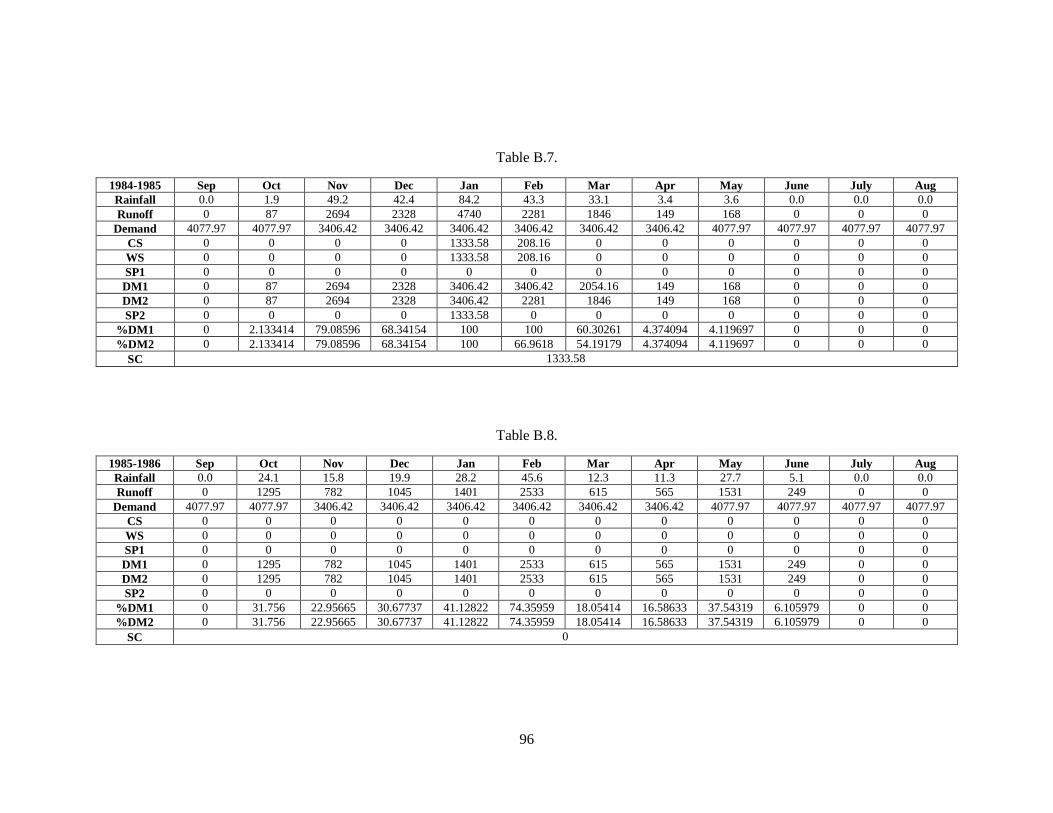
96
Table B.7.
1984-1985 Sep Oct Nov Dec Jan Feb Mar Apr May June July Aug
Rainfall 0.0 1.9 49.2 42.4 84.2 43.3 33.1 3.4 3.6 0.0 0.0 0.0
Runoff 0 87 2694 2328 4740 2281 1846 149 168 0 0 0
Demand 4077.97 4077.97 3406.42 3406.42 3406.42 3406.42 3406.42 3406.42 4077.97 4077.97 4077.97 4077.97
CS 0 0 0 0 1333.58 208.16 0 0 0 0 0 0
WS 0 0 0 0 1333.58 208.16 0 0 0 0 0 0
SP1 0 0 0 0 0 0 0 0 0 0 0 0
DM1 0 87 2694 2328 3406.42 3406.42 2054.16 149 168 0 0 0
DM2 0 87 2694 2328 3406.42 2281 1846 149 168 0 0 0
SP2 0 0 0 0 1333.58 0 0 0 0 0 0 0
%DM1 0 2.133414 79.08596 68.34154 100 100 60.30261 4.374094 4.119697 0 0 0
%DM2 0 2.133414 79.08596 68.34154 100 66.9618 54.19179 4.374094 4.119697 0 0 0
SC 1333.58
Table B.8.
1985-1986 Sep Oct Nov Dec Jan Feb Mar Apr May June July Aug
Rainfall 0.0 24.1 15.8 19.9 28.2 45.6 12.3 11.3 27.7 5.1 0.0 0.0
Runoff 0 1295 782 1045 1401 2533 615 565 1531 249 0 0
Demand 4077.97 4077.97 3406.42 3406.42 3406.42 3406.42 3406.42 3406.42 4077.97 4077.97 4077.97 4077.97
CS 0 0 0 0 0 0 0 0 0 0 0 0
WS 0 0 0 0 0 0 0 0 0 0 0 0
SP1 0 0 0 0 0 0 0 0 0 0 0 0
DM1 0 1295 782 1045 1401 2533 615 565 1531 249 0 0
DM2 0 1295 782 1045 1401 2533 615 565 1531 249 0 0
SP2 0 0 0 0 0 0 0 0 0 0 0 0
%DM1 0 31.756 22.95665 30.67737 41.12822 74.35959 18.05414 16.58633 37.54319 6.105979 0 0
%DM2 0 31.756 22.95665 30.67737 41.12822 74.35959 18.05414 16.58633 37.54319 6.105979 0 0
SC 0

97
Table B.9.
1986-1987 Sep Oct Nov Dec Jan Feb Mar Apr May June July Aug
Rainfall 0.2 11.6 131.1 26.8 57.8 17.0 89.3 2.4 2.8 1.6 0.0 0.0
Runoff 6 562 8219 1456 3192 870 5311 101 131 72 0 0
Demand 4077.97 4077.97 3406.42 3406.42 3406.42 3406.42 3406.42 3406.42 4077.97 4077.97 4077.97 4077.97
CS 0 0 4812.58 2862.16 2647.74 111.32 2015.9 0 0 0 0 0
WS 0 0 4812.58 2862.16 2647.74 111.32 2015.9 0 0 0 0 0
SP1 0 0 0 0 0 0 1904.58 0 0 0 0 0
DM1 6 562 3406.42 3406.42 3406.42 3406.42 3406.42 2116.9 131 72 0 0
DM2 6 562 3406.42 1456 3192 870 3406.42 101 131 72 0 0
SP2 0 0 4812.58 0 0 0 1904.58 0 0 0 0 0
%DM1 0.147132 13.78137 100 100 100 100 100 62.14442 3.212383 1.765584 0 0
%DM2 0.147132 13.78137 100 42.74282 93.70542 25.54001 100 2.96499 3.212383 1.765584 0 0
SC 4812.58
Table B.10.
1987-1988 Sep Oct Nov Dec Jan Feb Mar Apr May June July Aug
Rainfall 0.0 45.1 23.1 74.5 49.0 116.3 89.1 8.3 1.1 0.0 9.6 0.0
Runoff 0 2487 1202 4229 2703 7084 5098 379 44 0 494 0
Demand 4077.97 4077.97 3406.42 3406.42 3406.42 3406.42 3406.42 3406.42 4077.97 4077.97 4077.97 4077.97
CS 0 0 0 822.58 119.16 3796.74 5488.32 2460.9 0 0 0 0
WS 0 0 0 822.58 119.16 3796.74 5488.32 2460.9 0 0 0 0
SP1 0 0 0 0 0 3677.58 1691.58 0 0 0 0 0
DM1 0 2487 1202 3406.42 3406.42 3406.42 3406.42 3406.42 4077.97 0 494 0
DM2 0 2487 1202 3406.42 2703 3406.42 3406.42 379 44 0 494 0
SP2 0 0 0 822.58 0 3677.58 1691.58 0 0 0 0 0
%DM1 0 60.98623 35.28631 100 100 100 100 100 100 0 12.11387 0
%DM2 0 60.98623 35.28631 100 79.35017 100 100 11.12605 1.078968 0 12.11387 0
SC 5488.32

98
Table B.11.
1988-1989 Sep Oct Nov Dec Jan Feb Mar Apr May June July Aug
Rainfall 0.0 32.6 47.6 116.5 50.3 9.5 16.7 0.0 0.7 0.0 0.0 0.0
Runoff 0 1873 2601 7108 2889 490 848 0 30 0 0 0
Demand 4077.97 4077.97 3406.42 3406.42 3406.42 3406.42 3406.42 3406.42 4077.97 4077.97 4077.97 4077.97
CS 0 0 0 3701.58 3184.16 267.74 0 0 0 0 0 0
WS 0 0 0 3701.58 3184.16 267.74 0 0 0 0 0 0
SP1 0 0 0 0 0 0 0 0 0 0 0 0
DM1 0 1873 2601 3406.42 3406.42 3406.42 3406.42 0 30 0 0 0
DM2 0 1873 2601 3406.42 2889 490 848 0 30 0 0 0
SP2 0 0 0 3701.58 0 0 0 0 0 0 0 0
%DM1 0 45.92972 76.35582 100 100 100 100 0 0.73566 0 0 0
%DM2 0 45.92972 76.35582 100 84.81045 14.3846 24.89417 0 0.73566 0 0 0
SC 3701.58
Table B.12.
1989-1990 Sep Oct Nov Dec Jan Feb Mar Apr May June July Aug
Rainfall 0.0 20.0 25.5 18.3 13.6 70.5 25.4 0.5 0.0 4.0 0.0 0.0
Runoff 0 976 1352 908 690 4235 1401 22 0 123 0 0
Demand 4077.97 4077.97 3406.42 3406.42 3406.42 3406.42 3406.42 3406.42 4077.97 4077.97 4077.97 4077.97
CS 0 0 0 0 0 828.58 0 0 0 0 0 0
WS 0 0 0 0 0 828.58 0 0 0 0 0 0
SP1 0 0 0 0 0 0 0 0 0 0 0 0
DM1 0 976 1352 908 690 3406.42 2229.58 22 0 123 0 0
DM2 0 976 1352 908 690 3406.42 1401 22 0 123 0 0
SP2 0 0 0 0 0 828.58 0 0 0 0 0 0
%DM1 0 23.93348 39.68976 26.65555 20.25587 100 65.45229 0.645839 0 3.016207 0 0
%DM2 0 23.93348 39.68976 26.65555 20.25587 100 41.12822 0.645839 0 3.016207 0 0
SC 828.58

99
Table B.13.
1990-1991 Sep Oct Nov Dec Jan Feb Mar Apr May June July Aug
Rainfall 0.0 12.5 3.5 19.9 60.0 34.8 31.0 9.6 3.5 0.0 0.0 0.0
Runoff 0 630 168 1001 3256 1869 1625 489 163 0 0 0
Demand 4077.97 4077.97 3406.42 3406.42 3406.42 3406.42 3406.42 3406.42 4077.97 4077.97 4077.97 4077.97
CS 0 0 0 0 0 0 0 0 0 0 0 0
WS 0 0 0 0 0 0 0 0 0 0 0 0
SP1 0 0 0 0 0 0 0 0 0 0 0 0
DM1 0 630 168 1001 3256 1869 1625 489 163 0 0 0
DM2 0 630 168 1001 3256 1869 1625 489 163 0 0 0
SP2 0 0 0 0 0 0 0 0 0 0 0 0
%DM1 0 15.44886 4.931864 29.38569 95.58422 54.86699 47.70404 14.35525 3.997087 0 0 0
%DM2 0 15.44886 4.931864 29.38569 95.58422 54.86699 47.70404 14.35525 3.997087 0 0 0
SC 0
Table B.14.
1991-1992 Sep Oct Nov Dec Jan Feb Mar Apr May June July Aug
Rainfall 0.0 14.0 36.6 128.3 17.2 99.8 35.5 5.9 8.4 3.5 0.0 0.0
Runoff 0 697 2003 7689 837 5959 1892 285 419 168 0 0
Demand 4077.97 4077.97 3406.42 3406.42 3406.42 3406.42 3406.42 3406.42 4077.97 4077.97 4077.97 4077.97
CS 0 0 0 4282.58 1713.16 4265.74 2751.32 0 0 0 0 0
WS 0 0 0 4282.58 1713.16 4265.74 2751.32 0 0 0 0 0
SP1 0 0 0 0 0 0 0 0 0 0 0 0
DM1 0 697 2003 3406.42 3406.42 3406.42 3406.42 3036.32 419 168 0 0
DM2 0 697 2003 3406.42 837 3406.42 1892 285 419 168 0 0
SP2 0 0 0 4282.58 0 2552.58 0 0 0 0 0 0
%DM1 0 17.09184 58.80074 100 100 100 100 89.13522 10.27472 4.119697 0 0
%DM2 0 17.09184 58.80074 100 24.57125 100 55.54218 8.366555 10.27472 4.119697 0 0
SC 4282.58

100
Table B.15.
1992-1993 Sep Oct Nov Dec Jan Feb Mar Apr May June July Aug
Rainfall 0.0 0.8 51.4 80.3 38.6 51.8 45.9 3.6 12.0 0.0 0.0 0.0
Runoff 0 33 3046 4680 2110 2854 2578 168 580 0 0 0
Demand 4077.97 4077.97 3406.42 3406.42 3406.42 3406.42 3406.42 3406.42 4077.97 4077.97 4077.97 4077.97
CS 0 0 0 1273.58 0 0 0 0 0 0 0 0
WS 0 0 0 1273.58 0 0 0 0 0 0 0 0
SP1 0 0 0 0 0 0 0 0 0 0 0 0
DM1 0 33 3046 3406.42 3383.58 2854 2578 168 580 0 0 0
DM2 0 33 3046 3406.42 2110 2854 2578 168 580 0 0 0
SP2 0 0 0 1273.58 0 0 0 0 0 0 0 0
%DM1 0 0.809226 89.41939 100 99.3295 83.78297 75.68063 4.931864 14.22276 0 0 0
%DM2 0 0.809226 89.41939 100 61.94186 83.78297 75.68063 4.931864 14.22276 0 0 0
SC 1273.58
Table B.16.
1993-1994 Sep Oct Nov Dec Jan Feb Mar Apr May June July Aug
Rainfall 0.0 5.9 34.6 14.4 88.6 67.1 35.8 37.1 3.2 0.0 0.0 0.0
Runoff 0 288 1920 729 4953 3665 2016 2003 148 0 0 0
Demand 4077.97 4077.97 3406.42 3406.42 3406.42 3406.42 3406.42 3406.42 4077.97 4077.97 4077.97 4077.97
CS 0 0 0 0 1546.58 1805.16 414.74 0 0 0 0 0
WS 0 0 0 0 1546.58 1805.16 414.74 0 0 0 0 0
SP1 0 0 0 0 0 0 0 0 0 0 0 0
DM1 0 288 1920 729 3406.42 3406.42 3406.42 2417.74 1953.16 0 0 0
DM2 0 288 1920 729 3406.42 3406.42 2016 2003 148 0 0 0
SP2 0 0 0 0 1546.58 258.58 0 0 0 0 0 0
%DM1 0 7.062337 56.36416 21.40077 100 100 100 70.97598 3.629257 0 0 0
%DM2 0 7.062337 56.36416 21.40077 100 100 59.18237 58.80074 3.629257 0 0 0
SC 1805.16

101
Table B.17.
1994-1995 Sep Oct Nov Dec Jan Feb Mar Apr May June July Aug
Rainfall 42.0 61.2 99.3 50.5 20.8 13.1 13.0 30.4 10.5 0.0 0.4 0.0
Runoff 2469 3569 5871 2738 1054 677 636 1609 549 0 17 0
Demand 4077.97 4077.97 3406.42 3406.42 3406.42 3406.42 3406.42 3406.42 4077.97 4077.97 4077.97 4077.97
CS 0 0 2464.58 1796.16 0 0 0 0 0 0 0 0
WS 0 0 2464.58 1796.16 0 0 0 0 0 0 0 0
SP1 0 0 0 0 0 0 0 0 0 0 0 0
DM1 2469 3569 3406.42 3406.42 2850.16 677 636 1609 549 0 17 0
DM2 2469 3569 3406.42 2738 1054 677 636 1609 549 0 17 0
SP2 0 0 2464.58 0 0 0 0 0 0 0 0 0
%DM1 60.54483 87.51904 100 100 83.67025 19.87424 18.67063 47.23434 13.46258 0 0.416874 0
%DM2 60.54483 87.51904 100 80.37764 30.94158 19.87424 18.67063 47.23434 13.46258 0 0.416874 0
SC 2464.58
Table B.18.
1995-1996 Sep Oct Nov Dec Jan Feb Mar Apr May June July Aug
Rainfall 0.4 6.9 37.0 15.4 57.9 65.4 36.1 31.7 0.2 0.0 0.0 36.0
Runoff 14 327 2016 764 3310 3797 1885 1783 6 0 0 2117
Demand 4077.97 4077.97 3406.42 3406.42 3406.42 3406.42 3406.42 3406.42 4077.97 4077.97 4077.97 4077.97
CS 0 0 0 0 0 390.58 0 0 0 0 0 0
WS 0 0 0 0 0 390.58 0 0 0 0 0 0
SP1 0 0 0 0 0 0 0 0 0 0 0 0
DM1 14 327 2016 764 3310 3406.42 2275.58 1783 6 0 0 2117
DM2 14 327 2016 764 3310 3406.42 1885 1783 6 0 0 2117
SP2 0 0 0 0 0 390.58 0 0 0 0 0 0
%DM1 0.343308 8.018696 59.18237 22.42824 97.16946 100 66.80268 52.34234 0.147132 0 0 51.91308
%DM2 0.343308 8.018696 59.18237 22.42824 97.16946 100 55.33669 52.34234 0.147132 0 0 51.91308
SC 390.58

102
Table B.19.
1996-1997 Sep Oct Nov Dec Jan Feb Mar Apr May June July Aug
Rainfall 0.0 21.3 5.3 61.3 8.3 27.8 29.1 26.8 9.4 0.0 0.0 0.0
Runoff 0 1079 260 3414 408 1526 1499 1476 481 0 0 0
Demand 4077.97 4077.97 3406.42 3406.42 3406.42 3406.42 3406.42 3406.42 4077.97 4077.97 4077.97 4077.97
CS 0 0 0 7.58 0 0 0 0 0 0 0 0
WS 0 0 0 7.58 0 0 0 0 0 0 0 0
SP1 0 0 0 0 0 0 0 0 0 0 0 0
DM1 0 1079 260 3406.42 415.58 1526 1499 1476 481 0 0 0
DM2 0 1079 260 3406.42 408 1526 1499 1476 481 0 0 0
SP2 0 0 0 7.58 0 0 0 0 0 0 0 0
%DM1 0 26.45924 7.632647 100 12.1999 44.79776 44.00514 43.32995 11.79508 0 0 0
%DM2 0 26.45924 7.632647 100 11.97738 44.79776 44.00514 43.32995 11.79508 0 0 0
SC 7.58
Table B.20.
1997-1998 Sep Oct Nov Dec Jan Feb Mar Apr May June July Aug
Rainfall 14.0 22.3 82.5 57.9 31.5 13.9 42.2 5.2 7.9 0.0 0.0 0.0
Runoff 747 1141 4846 3230 1601 693 2361 242 372 0 0 0
Demand 4077.97 4077.97 3406.42 3406.42 3406.42 3406.42 3406.42 3406.42 4077.97 4077.97 4077.97 4077.97
CS 0 0 1439.58 1263.16 0 0 0 0 0 0 0 0
WS 0 0 1439.58 1263.16 0 0 0 0 0 0 0 0
SP1 0 0 0 0 0 0 0 0 0 0 0 0
DM1 747 1141 3406.42 3406.42 2864.16 693 2361 242 372 0 0 0
DM2 747 1141 3406.42 3230 1601 693 2361 242 372 0 0 0
SP2 0 0 1439.58 0 0 0 0 0 0 0 0 0
%DM1 18.31794 27.97961 100 100 84.08123 20.34394 69.3103 7.104233 9.122186 0 0 0
%DM2 18.31794 27.97961 100 94.82096 46.99949 20.34394 69.3103 7.104233 9.122186 0 0 0
SC 1439.58

103
Table B.21.
1998-1999 Sep Oct Nov Dec Jan Feb Mar Apr May June July Aug
Rainfall 0.0 1.0 31.7 86.4 102.9 30.7 31.8 39.6 0.0 0.0 0.0 0.0
Runoff 0 44 1643 4977 6236 1673 1711 2294 0 0 0 0
Demand 4077.97 4077.97 3406.42 3406.42 3406.42 3406.42 3406.42 3406.42 4077.97 4077.97 4077.97 4077.97
CS 0 0 0 1570.58 4400.16 2666.74 971.32 0 0 0 0 0
WS 0 0 0 1570.58 4400.16 2666.74 971.32 0 0 0 0 0
SP1 0 0 0 0 2829.58 0 0 0 0 0 0 0
DM1 0 44 1643 3406.42 3406.42 3406.42 3406.42 3265.32 0 0 0 0
DM2 0 44 1643 3406.42 3406.42 1673 1711 2294 0 0 0 0
SP2 0 0 0 1570.58 2829.58 0 0 0 0 0 0 0
%DM1 0 1.078968 48.23246 100 100 100 100 95.86782 0 0 0 0
%DM2 0 1.078968 48.23246 100 100 49.11315 50.22869 67.34343 0 0 0 0
SC 4400.16
Table B.22.
1999-2000 Sep Oct Nov Dec Jan Feb Mar Apr May June July Aug
Rainfall 1.4 1.0 18.2 33.1 39.0 70.1 28.6 25.3 4.1 0.0 0.0 0.0
Runoff 61 44 958 1811 1985 3923 1463 1300 194 0 0 0
Demand 4077.97 4077.97 3406.42 3406.42 3406.42 3406.42 3406.42 3406.42 4077.97 4077.97 4077.97 4077.97
CS 0 0 0 0 0 516.58 0 0 0 0 0 0
WS 0 0 0 0 0 516.58 0 0 0 0 0 0
SP1 0 0 0 0 0 0 0 0 0 0 0 0
DM1 61 44 958 1811 1985 3406.42 1979.58 1300 194 0 0 0
DM2 61 44 958 1811 1985 3406.42 1463 1300 194 0 0 0
SP2 0 0 0 0 0 516.58 0 0 0 0 0 0
%DM1 1.495842 1.078968 28.12337 53.16432 58.27232 100 58.11321 38.16323 4.757269 0 0 0
%DM2 1.495842 1.078968 28.12337 53.16432 58.27232 100 42.94832 38.16323 4.757269 0 0 0
SC 516.58
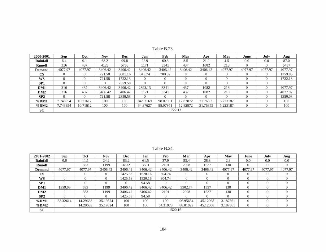
104
Table B.23.
2000-2001 Sep Oct Nov Dec Jan Feb Mar Apr May June July Aug
Rainfall 6.4 9.1 68.2 99.8 22.9 60.3 8.5 21.2 4.5 0.0 0.0 87.0
Runoff 316 437 4128 5766 1171 3341 437 1082 213 0 0 5437
Demand 4077.97 4077.97 3406.42 3406.42 3406.42 3406.42 3406.42 3406.42 4077.97 4077.97 4077.97 4077.97
CS 0 0 721.58 3081.16 845.74 780.32 0 0 0 0 0 1359.03
WS 0 0 721.58 1722.13 0 0 0 0 0 0 0 1722.13
SP1 0 0 0 2359.58 0 0 0 0 0 0 0 0
DM1 316 437 3406.42 3406.42 2893.13 3341 437 1082 213 0 0 4077.97
DM2 316 437 3406.42 3406.42 1171 3341 437 1082 213 0 0 4077.97
SP2 0 0 721.58 2359.58 0 0 0 0 0 0 0 1359.03
%DM1 7.748954 10.71612 100 100 84.93169 98.07951 12.82872 31.76355 5.223187 0 0 100
%DM2 7.748954 10.71612 100 100 34.37627 98.07951 12.82872 31.76355 5.223187 0 0 100
SC 1722.13
Table B.24.
2001-2002 Sep Oct Nov Dec Jan Feb Mar Apr May June July Aug
Rainfall 0.0 11.1 24.2 83.2 61.5 37.9 53.4 28.8 2.8 0.0 0.0 0.0
Runoff 0 583 1199 4832 3501 2191 2998 1537 130 0 0 0
Demand 4077.97 4077.97 3406.42 3406.42 3406.42 3406.42 3406.42 3406.42 4077.97 4077.97 4077.97 4077.97
CS 0 0 0 1425.58 1520.16 304.74 0 0 0 0 0 0
WS 0 0 0 1425.58 1520.16 304.74 0 0 0 0 0 0
SP1 0 0 0 0 94.58 0 0 0 0 0 0 0
DM1 1359.03 583 1199 3406.42 3406.42 3406.42 3302.74 1537 130 0 0 0
DM2 0 583 1199 3406.42 3406.42 2191 2998 1537 130 0 0 0
SP2 0 0 0 1425.58 94.58 0 0 0 0 0 0 0
%DM1 33.32614 14.29633 35.19824 100 100 100 96.95634 45.12068 3.187861 0 0 0
%DM2 0 14.29633 35.19824 100 100 64.31973 88.01029 45.12068 3.187861 0 0 0
SC 1520.16

105
Table B.25.
2002-2003 Sep Oct Nov Dec Jan Feb Mar Apr May June July Aug
Rainfall 8.5 12.2 67.9 107.1 53.2 159.0 71.4 11.1 0.1 3.3 0.0 0.0
Runoff 436 6332 3904 5854 2989 9829 4024 557 3 156 0 0
Demand 4077.97 4077.97 3406.42 3406.42 3406.42 3406.42 3406.42 3406.42 4077.97 4077.97 4077.97 4077.97
CS 0 2254.03 2751.61 5199.19 4781.77 11204.35 11821.9 8972.51 4897.54 975.57 0 0
WS 0 2254.03 2751.61 5199.19 4781.77 11204.35 11821.9 8972.51 4897.54 975.57 0 0
SP1 0 0 497.58 2447.58 0 6422.58 617.58 0 0 0 0 0
DM1 436 4077.97 3406.42 3406.42 3406.42 3406.42 3406.42 3406.42 4077.97 4077.97 975.57 0
DM2 436 4077.97 3406.42 3406.42 2989 3406.42 3406.42 557 3 156 0 0
SP2 0 2254.03 497.58 2447.58 0 6422.58 617.58 0 0 0 0 0
%DM1 10.69159 100 100 100 100 100 100 100 100 100 23.92293 0
%DM2 10.69159 100 100 100 87.74608 100 100 16.35148 0.073566 3.825433 0 0
SC 11821.9
Table B.26.
2003-2004 Sep Oct Nov Dec Jan Feb Mar Apr May June July Aug
Rainfall 0.0 26.2 37.8 37.1 135.3 55.2 0.01 8.1 3.2 0.4 0.0 0.0
Runoff 0 1444 2146 2146 8102 3046 0 409 150 17 0 0
Demand 4077.97 4077.97 3406.42 3406.42 3406.42 3406.42 3406.42 3406.42 4077.97 4077.97 4077.97 4077.97
CS 0 0 0 0 4695.58 4335.16 928.74 0 0 0 0 0
WS 0 0 0 0 4695.58 4335.16 928.74 0 0 0 0 0
SP1 0 0 0 0 0 0 0 0 0 0 0 0
DM1 0 1444 2146 2146 3406.42 3406.42 3406.42 1337.74 150 17 0 0
DM2 0 1444 2146 2146 3406.42 3046 0 409 150 17 0 0
SP2 0 0 0 0 4695.58 0 0 0 0 0 0 0
%DM1 0 35.40977 62.99869 62.99869 100 100 100 39.27114 3.678301 0.416874 0 0
%DM2 0 35.40977 62.99869 62.99869 100 89.41939 0 12.00674 3.678301 0.416874 0 0
SC 4695.58

106
Table B.27.
2004-2005 Sep Oct Nov Dec Jan Feb Mar Apr May June July Aug
Rainfall 0.0 32.2 46.9 51.6 36.8 40.8 28.8 27.9 1.1 1.0 0.0 0.0
Runoff 0 1877 2577 2865 1953 2427 1665 1598 44 44 0 0
Demand 4077.97 4077.97 3406.42 3406.42 3406.42 3406.42 3406.42 3406.42 4077.97 4077.97 4077.97 4077.97
CS 0 0 0 0 0 0 0 0 0 0 0 0
WS 0 0 0 0 0 0 0 0 0 0 0 0
SP1 0 0 0 0 0 0 0 0 0 0 0 0
DM1 0 1877 2577 2865 1953 2427 1665 1598 44 44 0 0
DM2 0 1877 2577 2865 1953 2427 1665 1598 44 44 0 0
SP2 0 0 0 0 0 0 0 0 0 0 0 0
%DM1 0 46.0278 75.65127 84.10589 57.33292 71.24782 48.87829 46.91142 1.078968 1.078968 0 0
%DM2 0 46.0278 75.65127 84.10589 57.33292 71.24782 48.87829 46.91142 1.078968 1.078968 0 0
SC 0
Table B.28.
2005-2006 Sep Oct Nov Dec Jan Feb Mar Apr May June July Aug
Rainfall 0.0 18.5 46.3 10.7 70.6 29.4 24.6 32.6 3.7 0.0 0.01 0.0
Runoff 0 958 2525 529 4059 1677 1276 1852 174 0 0 0
Demand 4077.97 4077.97 3406.42 3406.42 3406.42 3406.42 3406.42 3406.42 4077.97 4077.97 4077.97 4077.97
CS 0 0 0 0 652.58 0 0 0 0 0 0 0
WS 0 0 0 0 652.58 0 0 0 0 0 0 0
SP1 0 0 0 0 0 0 0 0 0 0 0 0
DM1 0 958 2525 529 3406.42 2329.58 1276 1852 174 0 0 0
DM2 0 958 2525 529 3406.42 1677 1276 1852 174 0 0 0
SP2 0 0 0 0 652.58 0 0 0 0 0 0 0
%DM1 0 23.49208 74.12474 15.5295 100 68.38793 37.45868 54.36793 4.266829 0 0 0
%DM2 0 23.49208 74.12474 15.5295 100 49.23057 37.45868 54.36793 4.266829 0 0 0
SC 652.58

107
Table B.29.
2006-2007 Sep Oct Nov Dec Jan Feb Mar Apr May June July Aug
Rainfall 0.4 45.8 14.6 3.7 34.7 75.1 27.1 7.8 84.1 1.0 0.0 0.0
Runoff 16 2543 736 171 1839 4224 1517 382 5168 44 0 0
Demand 4077.97 4077.97 3406.42 3406.42 3406.42 3406.42 3406.42 3406.42 4077.97 4077.97 4077.97 4077.97
CS 0 0 0 0 0 817.58 0 0 1090.03 0 0 0
WS 0 0 0 0 0 817.58 0 0 1090.03 0 0 0
SP1 0 0 0 0 0 0 0 0 0 0 0 0
DM1 16 2543 736 171 1839 3406.42 2334.58 382 4077.97 1134.03 0 0
DM2 16 2543 736 171 1839 3406.42 1517 382 4077.97 44 0 0
SP2 0 0 0 0 0 817.58 0 0 1090.03 0 0 0
%DM1 0.392352 62.35946 21.60626 5.019933 53.9863 100 68.53471 11.21412 100 27.80869 0 0
%DM2 0.392352 62.35946 21.60626 5.019933 53.9863 100 44.53356 11.21412 100 1.078968 0 0
SC 1090.03
Table B.30.
2007-2008 Sep Oct Nov Dec Jan Feb Mar Apr May June July Aug
Rainfall 0.0 0.0 33.5 40.1 15.4 31.0 7.1 1.5 3.5 0.0 0.0 0.0
Runoff 0 0 1936 2191 807 1708 331 68 168 0 0 0
Demand 4077.97 4077.97 3406.42 3406.42 3406.42 3406.42 3406.42 3406.42 4077.97 4077.97 4077.97 4077.97
CS 0 0 0 0 0 0 0 0 0 0 0 0
WS 0 0 0 0 0 0 0 0 0 0 0 0
SP1 0 0 0 0 0 0 0 0 0 0 0 0
DM1 0 0 1936 2191 807 1708 331 68 168 0 0 0
DM2 0 0 1936 2191 807 1708 331 68 168 0 0 0
SP2 0 0 0 0 0 0 0 0 0 0 0 0
%DM1 0 0 56.83386 64.31973 23.69056 50.14062 9.716946 1.996231 4.119697 0 0 0
%DM2 0 0 56.83386 64.31973 23.69056 50.14062 9.716946 1.996231 4.119697 0 0 0
SC 0

108
Table B.31.
2008-2009 Sep Oct Nov Dec Jan Feb Mar Apr May June July Aug
Rainfall 4.5 13.9 0.7 57.7 76.4 75.6 39.7 14.9 6.9 0.0 0.0 0.0
Runoff 212 699 30 3376 4431 4430 2113 788 332 0 0 0
Demand 4077.97 4077.97 3406.42 3406.42 3406.42 3406.42 3406.42 3406.42 4077.97 4077.97 4077.97 4077.97
CS 0 0 0 0 1024.58 2048.16 754.74 0 0 0 0 0
WS 0 0 0 0 1024.58 2048.16 754.74 0 0 0 0 0
SP1 0 0 0 0 0 1023.58 0 0 0 0 0 0
DM1 212 699 30 3376 3406.42 3406.42 3406.42 1542.74 332 0 0 0
DM2 212 699 30 3376 3406.42 3406.42 2113 788 332 0 0 0
SP2 0 0 0 0 1024.58 1023.58 0 0 0 0 0 0
%DM1 5.198665 17.14088 0.88069 99.10698 100 100 100 45.28919 8.141306 0 0 0
%DM2 5.198665 17.14088 0.88069 99.10698 100 100 62.02993 23.13279 8.141306 0 0 0
SC 2048.16
Tables B.32 to B.63 show the tank volume calculations for Reservoir 2 previously discussed in Chapter V, pages 66-67.
Table B.32.
1978-1979 Sep Oct Nov Dec Jan Feb Mar Apr May June July Aug
Rainfall 0.0 29.0 8.0 91.1 36.6 23.0 26.6 6.7 6.3 9.6 0.0 0.0
Runoff 0 1913 496 6512 2454 1152 1737 400 383 569 0 0
Demand 4999.24 4999.24 3728.26 3728.26 3728.26 3728.26 3728.26 3728.26 4999.24 4999.24 4999.24 4999.24
CS 0 0 0 2783.74 1509.48 0 0 0 0 0 0 0
WS 0 0 0 2783.74 1509.48 0 0 0 0 0 0 0
SP1 0 0 0 2783.74 1509.48 0 0 0 0 0 0 0
DM1 0 1913 496 3728.26 3728.26 2661.48 1737 400 383 569 0 0
DM2 0 1913 496 3728.26 2454 1152 1737 400 383 569 0 0
SP2 0 0 0 2783.74 0 0 0 0 0 0 0 0
%DM1 0 38.265816 13.303793 100 100 71.386652 46.590098 10.728865 7.6611645 11.38173 0 0
%DM2 0 38.265816 13.303793 100 65.82159 30.899133 46.590098 10.728865 7.6611645 11.38173 0 0
SC 2783.74
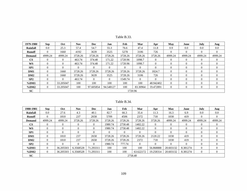
109
Table B.33.
1979-1980 Sep Oct Nov Dec Jan Feb Mar Apr May June July Aug
Rainfall 0.0 25.3 57.4 54.7 55.3 76.6 47.4 11.8 0.9 0.0 0.0 0.0
Runoff 0 1660 4192 3639 3525 5278 3106 726 0 0 0 0
Demand 4999.24 4999.24 3728.26 3728.26 3728.26 3728.26 3728.26 3728.26 4999.24 4999.24 4999.24 4999.24
CS 0 0 463.74 374.48 171.22 1720.96 1098.7 0 0 0 0 0
WS 0 0 463.74 374.48 171.22 1720.96 1098.7 0 0 0 0 0
SP1 0 0 0 0 0 0 0 0 0 0 0 0
DM1 0 1660 3728.26 3728.26 3728.26 3728.26 3728.26 1824.7 0 0 0 0
DM2 0 1660 3728.26 3639 3525 3728.26 3106 726 0 0 0 0
SP2 0 0 463.74 0 0 1549.74 0 0 0 0 0 0
%DM1 0 33.205047 100 100 100 100 100 48.942402 0 0 0 0
%DM2 0 33.205047 100 97.605854 94.548127 100 83.30964 19.472891 0 0 0 0
SC 1720.96
Table B.34.
1980-1981 Sep Oct Nov Dec Jan Feb Mar Apr May June July Aug
Rainfall 0.0 27.6 4.3 40.1 82.7 66.3 35.4 11.3 16.3 6.9 0.0 0.0
Runoff 0 1810 237 2658 5709 4506 2372 718 1030 419 0 0
Demand 4999.24 4999.24 3728.26 3728.26 3728.26 3728.26 3728.26 3728.26 4999.24 4999.24 4999.24 4999.24
CS 0 0 0 0 1980.74 2758.48 1402.22 0 0 0 0 0
WS 0 0 0 0 1980.74 2758.48 1402.22 0 0 0 0 0
SP1 0 0 0 0 0 0 0 0 0 0 0 0
DM1 0 1810 237 2658 3728.26 3728.26 3728.26 2120.22 1030 419 0 0
DM2 0 1810 237 2658 3728.26 3728.26 2372 718 1030 419 0 0
SP2 0 0 0 0 1980.74 777.74 0 0 0 0 0 0
%DM1 0 36.205503 6.3568528 71.293311 100 100 100 56.868888 20.603132 8.381274 0 0
%DM2 0 36.205503 6.3568528 71.293311 100 100 63.622172 19.258314 20.603132 8.381274 0 0
SC 2758.48

110
Table B.35.
1981-1982 Sep Oct Nov Dec Jan Feb Mar Apr May June July Aug
Rainfall 0.0 1.5 38.8 33.4 33.6 47.7 80.2 10.9 0.2 58.8 0.01 0.0
Runoff 0 82 2612 2127 2206 3094 5526 679 7 4417 0 0
Demand 4999.24 4999.24 3728.26 3728.26 3728.26 3728.26 3728.26 3728.26 4999.24 4999.24 4999.24 4999.24
CS 0 0 0 0 0 0 1797.74 0 0 0 0 0
WS 0 0 0 0 0 0 1797.74 0 0 0 0 0
SP1 0 0 0 0 0 0 0 0 0 0 0 0
DM1 0 82 2612 2127 2206 3094 3728.26 2476.74 7 4417 0 0
DM2 0 82 2612 2127 2206 3094 3728.26 679 7 4417 0 0
SP2 0 0 0 0 0 0 1797.74 0 0 0 0 0
%DM1 0 1.6402493 70.059492 57.050742 59.169693 82.987774 100 66.431526 0.1400213 88.35343 0 0
%DM2 0 1.6402493 70.059492 57.050742 59.169693 82.987774 100 18.212249 0.1400213 88.35343 0 0
SC 1797.74
Table B.36.
1982-1983 Sep Oct Nov Dec Jan Feb Mar Apr May June July Aug
Rainfall 0.0 1.5 23.9 22.6 26.6 69.0 38.4 15.4 21.7 17.4 0.0 0.0
Runoff 0 83 1596 1449 1692 4853 2533 923 1460 1170 0 0
Demand 4999.24 4999.24 3728.26 3728.26 3728.26 3728.26 3728.26 3728.26 4999.24 4999.24 4999.24 4999.24
CS 0 0 0 0 0 1124.74 0 0 0 0 0 0
WS 0 0 0 0 0 1124.74 0 0 0 0 0 0
SP1 0 0 0 0 0 0 0 0 0 0 0 0
DM1 0 83 1596 1449 1692 3728.26 3657.74 923 1460 1170 0 0
DM2 0 83 1596 1449 1692 3728.26 2533 923 1460 1170 0 0
SP2 0 0 0 0 0 1124.74 0 0 0 0 0 0
%DM1 0 1.6602524 42.808173 38.865315 45.383101 100 98.108501 24.756857 29.204439 23.403557 0 0
%DM2 0 1.6602524 42.808173 38.865315 45.383101 100 67.940541 24.756857 29.204439 23.403557 0 0
SC 1124.74

111
Table B.37.
1983-1984 Sep Oct Nov Dec Jan Feb Mar Apr May June July Aug
Rainfall 0.0 17.3 29.1 40.1 35.6 13.4 29.3 49.5 0.0 0.0 0.0 0.0
Runoff 0 1151 1934 2561 2242 858 2029 3402 0 0 0 0
Demand 4999.24 4999.24 3728.26 3728.26 3728.26 3728.26 3728.26 3728.26 4999.24 4999.24 4999.24 4999.24
CS 0 0 0 0 0 0 0 0 0 0 0 0
WS 0 0 0 0 0 0 0 0 0 0 0 0
SP1 0 0 0 0 0 0 0 0 0 0 0 0
DM1 0 1151 1934 2561 2242 858 2029 3402 0 0 0 0
DM2 0 1151 1934 2561 2242 858 2029 3402 0 0 0 0
SP2 0 0 0 0 0 0 0 0 0 0 0 0
%DM1 0 23.0235 51.874065 68.691561 60.135291 23.013416 54.42217 91.249001 0 0 0 0
%DM2 0 23.0235 51.874065 68.691561 60.135291 23.013416 54.42217 91.249001 0 0 0 0
SC 0
Table B.38.
1984-1985 Sep Oct Nov Dec Jan Feb Mar Apr May June July Aug
Rainfall 0.0 1.9 49.2 42.4 84.2 43.3 33.1 3.4 3.6 0.0 0.0 0.0
Runoff 0 104 3294 2847 5826 2775 2262 178 202 0 0 0
Demand 4999.24 4999.24 3728.26 3728.26 3728.26 3728.26 3728.26 3728.26 4999.24 4999.24 4999.24 4999.24
CS 0 0 0 0 2097.74 1144.48 0 0 0 0 0 0
WS 0 0 0 0 2097.74 1144.48 0 0 0 0 0 0
SP1 0 0 0 0 0 0 0 0 0 0 0 0
DM1 0 104 3294 2847 3728.26 3728.26 3406.48 178 202 0 0 0
DM2 0 104 3294 2847 3728.26 2775 2262 178 202 0 0 0
SP2 0 0 0 0 2097.74 0 0 0 0 0 0 0
%DM1 0 2.0803162 88.352207 76.3627 100 100 91.369164 4.7743451 4.0406142 0 0 0
%DM2 0 2.0803162 88.352207 76.3627 100 74.431504 60.671734 4.7743451 4.0406142 0 0 0
SC 2097.74
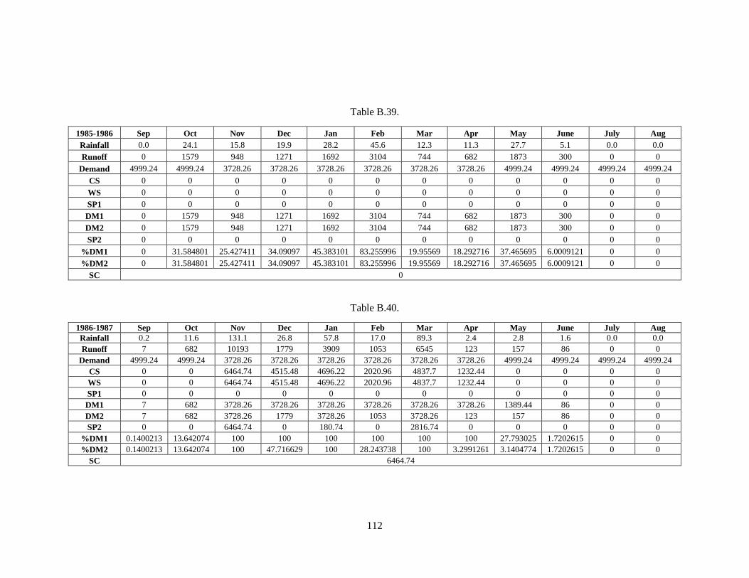
112
Table B.39.
1985-1986 Sep Oct Nov Dec Jan Feb Mar Apr May June July Aug
Rainfall 0.0 24.1 15.8 19.9 28.2 45.6 12.3 11.3 27.7 5.1 0.0 0.0
Runoff 0 1579 948 1271 1692 3104 744 682 1873 300 0 0
Demand 4999.24 4999.24 3728.26 3728.26 3728.26 3728.26 3728.26 3728.26 4999.24 4999.24 4999.24 4999.24
CS 0 0 0 0 0 0 0 0 0 0 0 0
WS 0 0 0 0 0 0 0 0 0 0 0 0
SP1 0 0 0 0 0 0 0 0 0 0 0 0
DM1 0 1579 948 1271 1692 3104 744 682 1873 300 0 0
DM2 0 1579 948 1271 1692 3104 744 682 1873 300 0 0
SP2 0 0 0 0 0 0 0 0 0 0 0 0
%DM1 0 31.584801 25.427411 34.09097 45.383101 83.255996 19.95569 18.292716 37.465695 6.0009121 0 0
%DM2 0 31.584801 25.427411 34.09097 45.383101 83.255996 19.95569 18.292716 37.465695 6.0009121 0 0
SC 0
Table B.40.
1986-1987 Sep Oct Nov Dec Jan Feb Mar Apr May June July Aug
Rainfall 0.2 11.6 131.1 26.8 57.8 17.0 89.3 2.4 2.8 1.6 0.0 0.0
Runoff 7 682 10193 1779 3909 1053 6545 123 157 86 0 0
Demand 4999.24 4999.24 3728.26 3728.26 3728.26 3728.26 3728.26 3728.26 4999.24 4999.24 4999.24 4999.24
CS 0 0 6464.74 4515.48 4696.22 2020.96 4837.7 1232.44 0 0 0 0
WS 0 0 6464.74 4515.48 4696.22 2020.96 4837.7 1232.44 0 0 0 0
SP1 0 0 0 0 0 0 0 0 0 0 0 0
DM1 7 682 3728.26 3728.26 3728.26 3728.26 3728.26 3728.26 1389.44 86 0 0
DM2 7 682 3728.26 1779 3728.26 1053 3728.26 123 157 86 0 0
SP2 0 0 6464.74 0 180.74 0 2816.74 0 0 0 0 0
%DM1 0.1400213 13.642074 100 100 100 100 100 100 27.793025 1.7202615 0 0
%DM2 0.1400213 13.642074 100 47.716629 100 28.243738 100 3.2991261 3.1404774 1.7202615 0 0
SC 6464.74

113
Table B.41.
1987-1988 Sep Oct Nov Dec Jan Feb Mar Apr May June July Aug
Rainfall 0.0 45.1 23.1 74.5 49.0 116.3 89.1 8.3 1.1 0.0 9.6 0.0
Runoff 0 3060 1462 5190 3311 8767 6266 459 53 0 602 0
Demand 4999.24 4999.24 3728.26 3728.26 3728.26 3728.26 3728.26 3728.26 4999.24 4999.24 4999.24 4999.24
CS 0 0 0 1461.74 1044.48 6083.22 8620.96 5351.7 405.46 0 0 0
WS 0 0 0 1461.74 1044.48 6083.22 8620.96 5351.7 405.46 0 0 0
SP1 0 0 0 0 0 0 0 0 0 0 0 0
DM1 0 3060 1462 3728.26 3728.26 3728.26 3728.26 3728.26 4999.24 405.46 602 0
DM2 0 3060 1462 3728.26 3311 3728.26 3728.26 459 53 0 602 0
SP2 0 0 0 1461.74 0 5038.74 2537.74 0 0 0 0 0
%DM1 0 61.209304 39.214003 100 100 100 100 100 100 8.1104328 12.04183 0
%DM2 0 61.209304 39.214003 100 88.808184 100 100 12.311373 1.0601611 0 12.04183 0
SC 8620.96
Table B.42.
1988-1989 Sep Oct Nov Dec Jan Feb Mar Apr May June July Aug
Rainfall 0.0 32.6 47.6 116.5 50.3 9.5 16.7 0.0 0.7 0.0 0.0 0.0
Runoff 0 2304 3180 8792 3552 595 1026 0 36 0 0 0
Demand 4999.24 4999.24 3728.26 3728.26 3728.26 3728.26 3728.26 3728.26 4999.24 4999.24 4999.24 4999.24
CS 0 0 0 5063.74 4887.48 1754.22 0 0 0 0 0 0
WS 0 0 0 5063.74 4887.48 1754.22 0 0 0 0 0 0
SP1 0 0 0 0 0 0 0 0 0 0 0 0
DM1 0 2304 3180 3728.26 3728.26 3728.26 2780.22 0 36 0 0 0
DM2 0 2304 3180 3728.26 3552 595 1026 0 36 0 0 0
SP2 0 0 0 5063.74 0 0 0 0 0 0 0 0
%DM1 0 46.087005 85.294481 100 100 100 74.571516 0 0.7201095 0 0 0
%DM2 0 46.087005 85.294481 100 95.272325 15.959187 27.51954 0 0.7201095 0 0 0
SC 5063.74

114
Table B.43.
1989-1990 Sep Oct Nov Dec Jan Feb Mar Apr May June July Aug
Rainfall 0.0 20.0 25.5 18.3 13.6 70.5 25.4 0.5 0.0 4.0 0.0 0.0
Runoff 0 1176 1646 1095 833 5232 1715 26 0 147 0 0
Demand 4999.24 4999.24 3728.26 3728.26 3728.26 3728.26 3728.26 3728.26 4999.24 4999.24 4999.24 4999.24
CS 0 0 0 0 0 1503.74 0 0 0 0 0 0
WS 0 0 0 0 0 1503.74 0 0 0 0 0 0
SP1 0 0 0 0 0 0 0 0 0 0 0 0
DM1 0 1176 1646 1095 833 3728.26 3218.74 26 0 147 0 0
DM2 0 1176 1646 1095 833 3728.26 1715 26 0 147 0 0
SP2 0 0 0 0 0 1503.74 0 0 0 0 0 0
%DM1 0 23.523576 44.149281 29.370269 22.342862 100 86.333571 0.6973763 0 2.9404469 0 0
%DM2 0 23.523576 44.149281 29.370269 22.342862 100 46.000011 0.6973763 0 2.9404469 0 0
SC 1503.74
Table B.44.
1990-1991 Sep Oct Nov Dec Jan Feb Mar Apr May June July Aug
Rainfall 0.0 12.5 3.5 19.9 60.0 34.8 31.0 9.6 3.5 0.0 0.0 0.0
Runoff 0 763 202 1209 3989 2276 1976 593 195 0 0 0
Demand 4999.24 4999.24 3728.26 3728.26 3728.26 3728.26 3728.26 3728.26 4999.24 4999.24 4999.24 4999.24
CS 0 0 0 0 260.74 0 0 0 0 0 0 0
WS 0 0 0 0 260.74 0 0 0 0 0 0 0
SP1 0 0 0 0 0 0 0 0 0 0 0 0
DM1 0 763 202 1209 3728.26 2536.74 1976 593 195 0 0 0
DM2 0 763 202 1209 3728.26 2276 1976 593 195 0 0 0
SP2 0 0 0 0 260.74 0 0 0 0 0 0 0
%DM1 0 15.26232 5.4180771 32.427996 100 68.040856 53.000595 15.905543 3.9005929 0 0 0
%DM2 0 15.26232 5.4180771 32.427996 100 61.047245 53.000595 15.905543 3.9005929 0 0 0
SC 260.74

115
Table B.45.
1991-1992 Sep Oct Nov Dec Jan Feb Mar Apr May June July Aug
Rainfall 0.0 14.0 36.6 128.3 17.2 99.8 35.5 5.9 8.4 3.5 0.0 0.0
Runoff 0 844 2464 9519 1016 7357 2304 343 505 202 0 0
Demand 4999.24 4999.24 3728.26 3728.26 3728.26 3728.26 3728.26 3728.26 4999.24 4999.24 4999.24 4999.24
CS 0 0 0 5790.74 3078.48 6707.22 5282.96 1897.7 0 0 0 0
WS 0 0 0 5790.74 3078.48 6707.22 5282.96 1897.7 0 0 0 0
SP1 0 0 0 0 0 0 0 0 0 0 0 0
DM1 0 844 2464 3728.26 3728.26 3728.26 3728.26 3728.26 2402.7 202 0 0
DM2 0 844 2464 3728.26 1016 3728.26 2304 343 505 202 0 0
SP2 0 0 0 5790.74 0 3628.74 0 0 0 0 0 0
%DM1 0 16.882566 66.089811 100 100 100 100 100 48.061305 4.0406142 0 0
%DM2 0 16.882566 66.089811 100 27.251318 100 61.798265 9.2000021 10.101535 4.0406142 0 0
SC 6707.22
Table B.46.
1992-1993 Sep Oct Nov Dec Jan Feb Mar Apr May June July Aug
Rainfall 0.0 0.8 51.4 80.3 38.6 51.8 45.9 3.6 12.0 0.0 0.0 0.0
Runoff 0 39 3758 5765 2582 3492 3161 201 697 0 0 0
Demand 4999.24 4999.24 3728.26 3728.26 3728.26 3728.26 3728.26 3728.26 4999.24 4999.24 4999.24 4999.24
CS 0 0 29.74 2066.48 920.22 683.96 116.7 0 0 0 0 0
WS 0 0 29.74 2066.48 920.22 683.96 116.7 0 0 0 0 0
SP1 0 0 0 0 0 0 0 0 0 0 0 0
DM1 0 39 3728.26 3728.26 3728.26 3728.26 3728.26 317.7 697 0 0 0
DM2 0 39 3728.26 3728.26 2582 3492 3161 201 697 0 0 0
SP2 0 0 29.74 2036.74 0 0 0 0 0 0 0 0
%DM1 0 0.7801186 100 100 100 100 100 8.5214014 13.942119 0 0 0
%DM2 0 0.7801186 100 100 69.254827 93.662996 84.784859 5.3912549 13.942119 0 0 0
SC 2066.48

116
Table B.47.
1993-1994 Sep Oct Nov Dec Jan Feb Mar Apr May June July Aug
Rainfall 0.0 5.9 34.6 14.4 88.6 67.1 35.8 37.1 3.2 0.0 0.0 0.0
Runoff 0 350 2353 882 6091 4481 2472 2477 176 0 0 0
Demand 4999.24 4999.24 3728.26 3728.26 3728.26 3728.26 3728.26 3728.26 4999.24 4999.24 4999.24 4999.24
CS 0 0 0 0 2362.74 3115.48 1859.22 607.96 0 0 0 0
WS 0 0 0 0 2362.74 3115.48 1859.22 607.96 0 0 0 0
SP1 0 0 0 0 0 0 0 0 0 0 0 0
DM1 0 350 2353 882 3728.26 3728.26 3728.26 3728.26 783.96 0 0 0
DM2 0 350 2353 882 3728.26 3728.26 2472 2477 176 0 0 0
SP2 0 0 0 0 2362.74 752.74 0 0 0 0 0 0
%DM1 0 7.0010642 63.112551 23.657148 100 100 100 100 15.681584 0 0 0
%DM2 0 7.0010642 63.112551 23.657148 100 100 66.304389 66.438499 3.5205351 0 0 0
SC 3115.48
Table B.48.
1994-1995 Sep Oct Nov Dec Jan Feb Mar Apr May June July Aug
Rainfall 42.0 61.2 99.3 50.5 20.8 13.1 13.0 30.4 10.5 0.0 0.4 0.0
Runoff 3047 4397 7258 3342 1274 821 767 1959 667 0 20 0
Demand 4999.24 4999.24 3728.26 3728.26 3728.26 3728.26 3728.26 3728.26 4999.24 4999.24 4999.24 4999.24
CS 0 0 3529.74 3143.48 689.22 0 0 0 0 0 0 0
WS 0 0 3529.74 3143.48 689.22 0 0 0 0 0 0 0
SP1 0 0 0 0 0 0 0 0 0 0 0 0
DM1 3047 4397 3728.26 3728.26 3728.26 1510.22 767 1959 667 0 20 0
DM2 3047 4397 3728.26 3342 1274 821 767 1959 667 0 20 0
SP2 0 0 3529.74 0 0 0 0 0 0 0 0 0
%DM1 60.949264 87.953369 100 100 100 40.507368 20.5726 52.544619 13.342028 0 0.4000608 0
%DM2 60.949264 87.953369 100 89.639671 34.171437 22.020996 20.5726 52.544619 13.342028 0 0.4000608 0
SC 3529.74

117
Table B.49.
1995-1996 Sep Oct Nov Dec Jan Feb Mar Apr May June July Aug
Rainfall 0.4 6.9 37.0 15.4 57.9 65.4 36.1 31.7 0.2 0.0 0.0 36.0
Runoff 18 392 2461 922 4065 4673 2290 2187 7 0 0 2611
Demand 4999.24 4999.24 3728.26 3728.26 3728.26 3728.26 3728.26 3728.26 4999.24 4999.24 4999.24 4999.24
CS 0 0 0 0 336.74 1281.48 0 0 0 0 0 0
WS 0 0 0 0 336.74 1281.48 0 0 0 0 0 0
SP1 0 0 0 0 0 0 0 0 0 0 0 0
DM1 18 392 2461 922 3728.26 3728.26 3571.48 2187 7 0 0 2611
DM2 18 392 2461 922 3728.26 3728.26 2290 2187 7 0 0 2611
SP2 0 0 0 0 336.74 944.74 0 0 0 0 0 0
%DM1 0.3600547 7.8411919 66.009345 24.730035 100 100 95.794821 58.660072 0.1400213 0 0 52.227939
%DM2 0.3600547 7.8411919 66.009345 24.730035 100 100 61.422755 58.660072 0.1400213 0 0 52.227939
SC 1281.48
Table B.50.
1996-1997 Sep Oct Nov Dec Jan Feb Mar Apr May June July Aug
Rainfall 0.0 21.3 5.3 61.3 8.3 27.8 29.1 26.8 9.4 0.0 0.0 0.0
Runoff 0 1307 314 4185 494 1866 1820 1805 584 0 0 0
Demand 4999.24 4999.24 3728.26 3728.26 3728.26 3728.26 3728.26 3728.26 4999.24 4999.24 4999.24 4999.24
CS 0 0 0 456.74 0 0 0 0 0 0 0 0
WS 0 0 0 456.74 0 0 0 0 0 0 0 0
SP1 0 0 0 0 0 0 0 0 0 0 0 0
DM1 0 1307 314 3728.26 950.74 1866 1820 1805 584 0 0 0
DM2 0 1307 314 3728.26 494 1866 1820 1805 584 0 0 0
SP2 0 0 0 456.74 0 0 0 0 0 0 0 0
%DM1 0 26.143974 8.4221594 100 25.500904 50.050157 48.816338 48.414005 11.681776 0 0 0
%DM2 0 26.143974 8.4221594 100 13.250149 50.050157 48.816338 48.414005 11.681776 0 0 0
SC 456.74
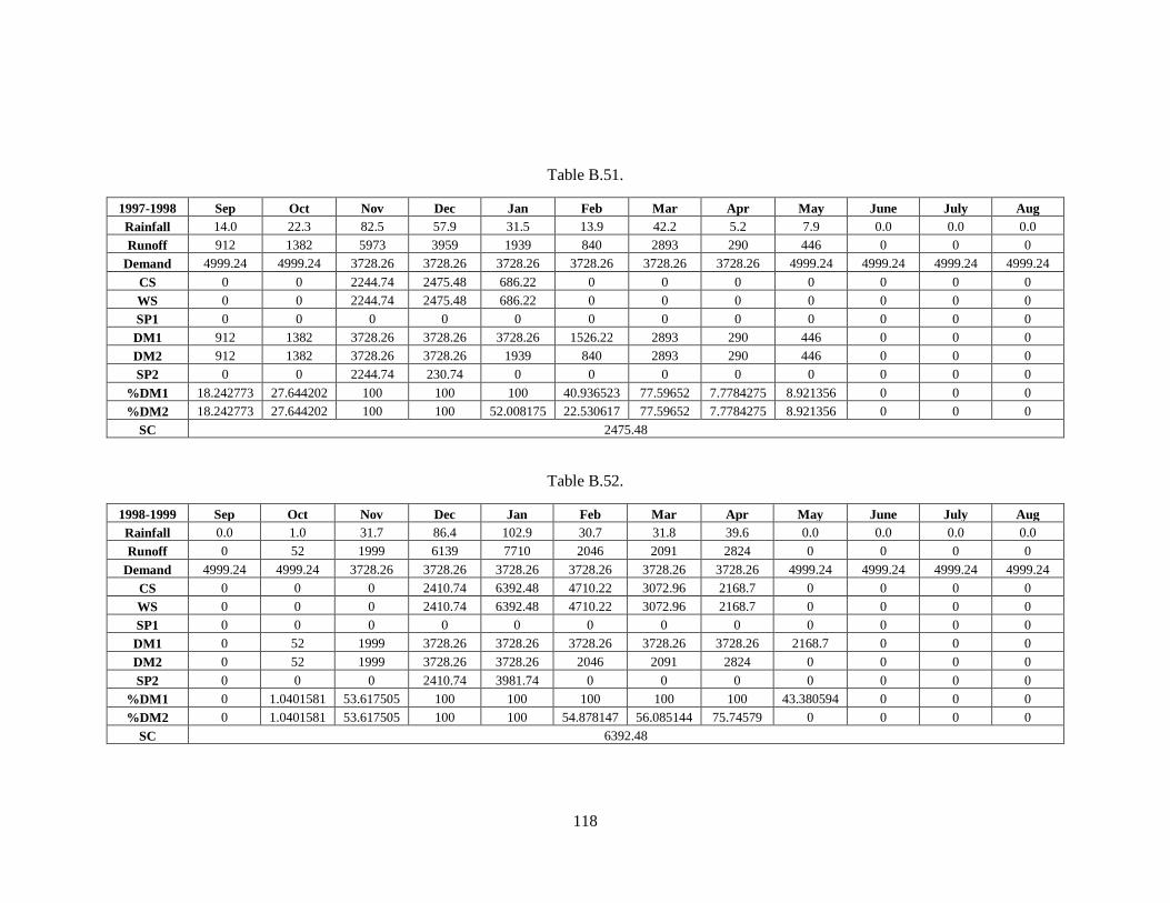
118
Table B.51.
1997-1998 Sep Oct Nov Dec Jan Feb Mar Apr May June July Aug
Rainfall 14.0 22.3 82.5 57.9 31.5 13.9 42.2 5.2 7.9 0.0 0.0 0.0
Runoff 912 1382 5973 3959 1939 840 2893 290 446 0 0 0
Demand 4999.24 4999.24 3728.26 3728.26 3728.26 3728.26 3728.26 3728.26 4999.24 4999.24 4999.24 4999.24
CS 0 0 2244.74 2475.48 686.22 0 0 0 0 0 0 0
WS 0 0 2244.74 2475.48 686.22 0 0 0 0 0 0 0
SP1 0 0 0 0 0 0 0 0 0 0 0 0
DM1 912 1382 3728.26 3728.26 3728.26 1526.22 2893 290 446 0 0 0
DM2 912 1382 3728.26 3728.26 1939 840 2893 290 446 0 0 0
SP2 0 0 2244.74 230.74 0 0 0 0 0 0 0 0
%DM1 18.242773 27.644202 100 100 100 40.936523 77.59652 7.7784275 8.921356 0 0 0
%DM2 18.242773 27.644202 100 100 52.008175 22.530617 77.59652 7.7784275 8.921356 0 0 0
SC 2475.48
Table B.52.
1998-1999 Sep Oct Nov Dec Jan Feb Mar Apr May June July Aug
Rainfall 0.0 1.0 31.7 86.4 102.9 30.7 31.8 39.6 0.0 0.0 0.0 0.0
Runoff 0 52 1999 6139 7710 2046 2091 2824 0 0 0 0
Demand 4999.24 4999.24 3728.26 3728.26 3728.26 3728.26 3728.26 3728.26 4999.24 4999.24 4999.24 4999.24
CS 0 0 0 2410.74 6392.48 4710.22 3072.96 2168.7 0 0 0 0
WS 0 0 0 2410.74 6392.48 4710.22 3072.96 2168.7 0 0 0 0
SP1 0 0 0 0 0 0 0 0 0 0 0 0
DM1 0 52 1999 3728.26 3728.26 3728.26 3728.26 3728.26 2168.7 0 0 0
DM2 0 52 1999 3728.26 3728.26 2046 2091 2824 0 0 0 0
SP2 0 0 0 2410.74 3981.74 0 0 0 0 0 0 0
%DM1 0 1.0401581 53.617505 100 100 100 100 100 43.380594 0 0 0
%DM2 0 1.0401581 53.617505 100 100 54.878147 56.085144 75.74579 0 0 0 0
SC 6392.48

119
Table B.53.
1999-2000 Sep Oct Nov Dec Jan Feb Mar Apr May June July Aug
Rainfall 1.4 1.0 18.2 33.1 39.0 70.1 28.6 25.3 4.1 0.0 0.0 0.0
Runoff 72 52 1165 2214 2410 4814 1773 1576 233 0 0 0
Demand 4999.24 4999.24 3728.26 3728.26 3728.26 3728.26 3728.26 3728.26 4999.24 4999.24 4999.24 4999.24
CS 0 0 0 0 0 1085.74 0 0 0 0 0 0
WS 0 0 0 0 0 1085.74 0 0 0 0 0 0
SP1 0 0 0 0 0 0 0 0 0 0 0 0
DM1 72 52 1165 2214 2410 3728.26 2858.74 1576 233 0 0 0
DM2 72 52 1165 2214 2410 3728.26 1773 1576 233 0 0 0
SP2 0 0 0 0 0 1085.74 0 0 0 0 0 0
%DM1 1.4402189 1.0401581 31.247821 59.38427 64.641414 100 76.677592 42.27173 4.6607084 0 0 0
%DM2 1.4402189 1.0401581 31.247821 59.38427 64.641414 100 47.555696 42.27173 4.6607084 0 0 0
SC 1085.74
Table B.54.
2000-2001 Sep Oct Nov Dec Jan Feb Mar Apr May June July Aug
Rainfall 6.4 9.1 68.2 99.8 22.9 60.3 8.5 21.2 4.5 0.0 0.0 87.0
Runoff 382 524 5112 7103 1418 4094 529 1311 255 0 0 6744
Demand 4999.24 4999.24 3728.26 3728.26 3728.26 3728.26 3728.26 3728.26 4999.24 4999.24 4999.24 4999.24
CS 0 0 1383.74 4758.48 2448.22 2813.96 0 0 0 0 0 1744.76
WS 0 0 1383.74 4758.48 2448.22 2813.96 0 0 0 0 0 1744.76
SP1 0 0 0 1744.76 0 0 0 0 0 0 0 0
DM1 382 524 3728.26 3728.26 3728.26 3728.26 3342.96 1311 255 0 0 4999.24
DM2 382 524 3728.26 3728.26 1418 3728.26 529 1311 255 0 0 4999.24
SP2 0 0 1383.74 3374.74 0 365.74 0 0 0 0 0 1744.76
%DM1 7.6411615 10.481593 100 100 100 100 89.66542 35.163857 5.1007753 0 0 100
%DM2 7.6411615 10.481593 100 100 38.033828 100 14.188925 35.163857 5.1007753 0 0 100
SC 3013.72

120
Table B.55.
2001-2002 Sep Oct Nov Dec Jan Feb Mar Apr May June July Aug
Rainfall 0.0 11.1 24.2 83.2 61.5 37.9 53.4 28.8 2.8 0.0 0.0 0.0
Runoff 0 710 1451 5949 4299 2696 3688 1874 154 0 0 0
Demand 4999.24 4999.24 3728.26 3728.26 3728.26 3728.26 3728.26 3728.26 4999.24 4999.24 4999.24 4999.24
CS 0 0 0 2220.74 2791.48 1759.22 1718.96 0 0 0 0 0
WS 0 0 0 2220.74 2791.48 1759.22 1718.96 0 0 0 0 0
SP1 0 0 0 0 0 0 0 0 0 0 0 0
DM1 1744.76 710 1451 3728.26 3728.26 3728.26 3728.26 3592.96 154 0 0 0
DM2 0 710 1451 3728.26 3728.26 2696 3688 1874 154 0 0 0
SP2 0 0 0 2220.74 570.74 0 0 0 0 0 0 0
%DM1 34.900505 14.202159 38.91896 100 100 100 100 96.370961 3.0804682 0 0 0
%DM2 0 14.202159 38.91896 100 100 72.312553 98.92014 50.264735 3.0804682 0 0 0
SC 2791.48
Table B.56.
2002-2003 Sep Oct Nov Dec Jan Feb Mar Apr May June July Aug
Rainfall 8.5 12.2 67.9 107.1 53.2 159.0 71.4 11.1 0.1 3.3 0.0 0.0
Runoff 529 767 4810 7208 3665 12192 4938 673 4 187 0 0
Demand 4999.24 4999.24 3728.26 3728.26 3728.26 3728.26 3728.26 3728.26 4999.24 4999.24 4999.24 4999.24
CS 0 0 1081.74 4561.48 4498.22 12961.96 14171.7 11116.44 6121.2 1308.96 0 0
WS 0 0 1081.74 4561.48 4498.22 12961.96 14171.7 11116.44 6121.2 1308.96 0 0
SP1 0 0 0 0 0 0 0 0 0 0 0 0
DM1 529 767 3728.26 3728.26 3728.26 3728.26 3728.26 3728.26 4999.24 4999.24 1308.96 0
DM2 529 767 3728.26 3728.26 3665 3728.26 3728.26 673 4 187 0 0
SP2 0 0 1081.74 3479.74 0 8463.74 1209.74 0 0 0 0 0
%DM1 10.581608 15.342332 100 100 100 100 100 100 100 100 26.18318 0
%DM2 10.581608 15.342332 100 100 98.30323 100 100 18.051316 0.0800122 3.7405686 0 0
SC 14171.7

121
Table B.57.
2003-2004 Sep Oct Nov Dec Jan Feb Mar Apr May June July Aug
Rainfall 0.0 26.2 37.8 37.1 135.3 55.2 0.01 8.1 3.2 0.4 0.0 0.0
Runoff 0 1767 2636 2636 10023 3727 0 496 179 20 0 0
Demand 4999.24 4999.24 3728.26 3728.26 3728.26 3728.26 3728.26 3728.26 4999.24 4999.24 4999.24 4999.24
CS 0 0 0 0 6294.74 6293.48 2565.22 0 0 0 0 0
WS 0 0 0 0 6294.74 6293.48 2565.22 0 0 0 0 0
SP1 0 0 0 0 0 0 0 0 0 0 0 0
DM1 0 1767 2636 2636 3728.26 3728.26 3728.26 3061.22 179 20 0 0
DM2 0 1767 2636 2636 3728.26 3727 0 496 179 20 0 0
SP2 0 0 0 0 6294.74 0 0 0 0 0 0 0
%DM1 0 35.345372 70.703223 70.703223 100 100 100 82.108544 3.5805442 0.4000608 0 0
%DM2 0 35.345372 70.703223 70.703223 100 99.966204 0 13.303793 3.5805442 0.4000608 0 0
SC 6294.74
Table B.58.
2004-2005 Sep Oct Nov Dec Jan Feb Mar Apr May June July Aug
Rainfall 0.0 32.2 46.9 51.6 36.8 40.8 28.8 27.9 1.1 1.0 0.0 0.0
Runoff 0 2312 3153 3511 2385 2993 2048 1964 52 52 0 0
Demand 4999.24 4999.24 3728.26 3728.26 3728.26 3728.26 3728.26 3728.26 4999.24 4999.24 4999.24 4999.24
CS 0 0 0 0 0 0 0 0 0 0 0 0
WS 0 0 0 0 0 0 0 0 0 0 0 0
SP1 0 0 0 0 0 0 0 0 0 0 0 0
DM1 0 2312 3153 3511 2385 2993 2048 1964 52 52 0 0
DM2 0 2312 3153 3511 2385 2993 2048 1964 52 52 0 0
SP2 0 0 0 0 0 0 0 0 0 0 0 0
%DM1 0 46.24703 84.570282 94.172617 63.97086 80.278736 54.931791 52.678729 1.0401581 1.0401581 0 0
%DM2 0 46.24703 84.570282 94.172617 63.97086 80.278736 54.931791 52.678729 1.0401581 1.0401581 0 0
SC 0

122
Table B.59.
2005-2006 Sep Oct Nov Dec Jan Feb Mar Apr May June July Aug
Rainfall 0.0 18.5 46.3 10.7 70.6 29.4 24.6 32.6 3.7 0.0 0.01 0.0
Runoff 0 1166 3086 637 4993 2059 1548 2275 208 0 0 0
Demand 4999.24 4999.24 3728.26 3728.26 3728.26 3728.26 3728.26 3728.26 4999.24 4999.24 4999.24 4999.24
CS 0 0 0 0 1264.74 0 0 0 0 0 0 0
WS 0 0 0 0 1264.74 0 0 0 0 0 0 0
SP1 0 0 0 0 0 0 0 0 0 0 0 0
DM1 0 1166 3086 637 3728.26 3323.74 1548 2275 208 0 0 0
DM2 0 1166 3086 637 3728.26 2059 1548 2275 208 0 0 0
SP2 0 0 0 0 1264.74 0 0 0 0 0 0 0
%DM1 0 23.323545 82.773197 17.085718 100 89.149898 41.520709 61.020422 4.1606324 0 0 0
%DM2 0 23.323545 82.773197 17.085718 100 55.226835 41.520709 61.020422 4.1606324 0 0 0
SC 1264.74
Table B.60.
2006-2007 Sep Oct Nov Dec Jan Feb Mar Apr May June July Aug
Rainfall 0.4 45.8 14.6 3.7 34.7 75.1 27.1 7.8 84.1 1.0 0.0 0.0
Runoff 20 3148 889 204 2242 5203 1859 459 6396 52 0 0
Demand 4999.24 4999.24 3728.26 3728.26 3728.26 3728.26 3728.26 3728.26 4999.24 4999.24 4999.24 4999.24
CS 0 0 0 0 0 1474.74 0 0 1396.76 0 0 0
WS 0 0 0 0 0 1474.74 0 0 1396.76 0 0 0
SP1 0 0 0 0 0 0 0 0 0 0 0 0
DM1 20 3148 889 204 2242 3728.26 3333.74 459 4999.24 1448.76 0 0
DM2 20 3148 889 204 2242 3728.26 1859 459 4999.24 52 0 0
SP2 0 0 0 0 0 1474.74 0 0 1396.76 0 0 0
%DM1 0.4000608 62.969571 23.844904 5.4717214 60.135291 100 89.41812 12.311373 100 28.979605 0 0
%DM2 0.4000608 62.969571 23.844904 5.4717214 60.135291 100 49.862402 12.311373 100 1.0401581 0 0
SC 1474.74

123
Table B.61.
2007-2008 Sep Oct Nov Dec Jan Feb Mar Apr May June July Aug
Rainfall 0.0 0.0 33.5 40.1 15.4 31.0 7.1 1.5 3.5 0.0 0.0 0.0
Runoff 0 0 2381 2677 982 2092 399 81 202 0 0 0
Demand 4999.24 4999.24 3728.26 3728.26 3728.26 3728.26 3728.26 3728.26 4999.24 4999.24 4999.24 4999.24
CS 0 0 0 0 0 0 0 0 0 0 0 0
WS 0 0 0 0 0 0 0 0 0 0 0 0
SP1 0 0 0 0 0 0 0 0 0 0 0 0
DM1 0 0 2381 2677 982 2092 399 81 202 0 0 0
DM2 0 0 2381 2677 982 2092 399 81 202 0 0 0
SP2 0 0 0 0 0 0 0 0 0 0 0 0
%DM1 0 0 63.863572 71.802932 26.339365 56.111966 10.702043 2.1725953 4.0406142 0 0 0
%DM2 0 0 63.863572 71.802932 26.339365 56.111966 10.702043 2.1725953 4.0406142 0 0 0
SC 0
Table B.62.
2008-2009 Sep Oct Nov Dec Jan Feb Mar Apr May June July Aug
Rainfall 4.5 13.9 0.7 57.7 76.4 75.6 39.7 14.9 6.9 0.0 0.0 0.0
Runoff 256 846 36 4166 5467 5461 2572 951 399 0 0 0
Demand 4999.24 4999.24 3728.26 3728.26 3728.26 3728.26 3728.26 3728.26 4999.24 4999.24 4999.24 4999.24
CS 0 0 0 437.74 2176.48 3909.22 2752.96 0 0 0 0 0
WS 0 0 0 437.74 2176.48 3909.22 2752.96 0 0 0 0 0
SP1 0 0 0 0 0 0 0 0 0 0 0 0
DM1 256 846 36 3728.26 3728.26 3728.26 3728.26 3703.96 399 0 0 0
DM2 256 846 36 3728.26 3728.26 3728.26 2572 951 399 0 0 0
SP2 0 0 0 437.74 1738.74 1732.74 0 0 0 0 0 0
%DM1 5.1207784 16.922572 0.9655979 100 100 100 100 99.348221 7.9812131 0 0 0
%DM2 5.1207784 16.922572 0.9655979 100 100 100 68.986605 25.507878 7.9812131 0 0 0
SC 3909.22

124
Tables B.63 to B.93 show the tank volume calculations for Reservoir 3 previously discussed in Chapter V, pages 66-67.
Table B.63.
1978-1979 Sep Oct Nov Dec Jan Feb Mar Apr May June July Aug
Rainfall 0.0 29.0 8.0 91.1 36.6 23.0 26.6 6.7 6.3 9.6 0.0 0.0
Runoff 0 4314 1132 15190 5664 2664 3997 908 870 1291 0 0
Demand 368.8 368.8 0.0 0.0 0.0 0.0 368.8 368.8 368.8 368.8 368.8 368.8
CS 0 3945.2 5077.2 20267.2 25931.2 28595.2 32223.4 32762.6 33263.8 34186 33817.2 33448.4
WS 0 737.6 737.6 737.6 737.6 737.6 737.6 737.6 737.6 737.6 368.8 5.798E-12
SP1 0 3945.2 1869.6 15927.6 6401.6 3401.6 4365.8 1276.8 1238.8 1659.8 368.8 5.798E-12
DM1 0 368.8 0 0 0 0 368.8 368.8 368.8 368.8 368.8 368.8
DM2 0 368.8 0 0 0 0 368.8 368.8 368.8 368.8 0 0
SP2 0 3945.2 1132 15190 5664 2664 3628.2 539.2 501.2 922.2 0 0
%DM1 0 100 100 100 100 100 100 100 100 100 100 100
%DM2 0 100 100 100 100 100 100 100 100 100 0 0
SC 737.6
Table B.64.
1979-1980 Sep Oct Nov Dec Jan Feb Mar Apr May June July Aug
Rainfall 0.0 25.3 57.4 54.7 55.3 76.6 47.4 11.8 0.9 0.0 0.0 0.0
Runoff 0 3823 9777 8398 8071 12194 7155 1655 0 0 0 0
Demand 368.8 368.8 0.0 0.0 0.0 0.0 368.8 368.8 368.8 368.8 368.8 368.8
CS 33079.6 36533.8 46310.8 54708.8 62779.8 74973.8 81760 83046.2 82677.4 82308.6 81939.8 81571
WS 0 1475.2 1475.2 1475.2 1475.2 1475.2 1475.2 1475.2 1106.4 737.6 368.8 1.171E-11
SP1 0 1979 9777 8398 8071 12194 6786.2 1286.2 0 0 0 0
DM1 5.798E-12 368.8 0 0 0 0 368.8 368.8 368.8 368.8 368.8 368.8
DM2 0 368.8 0 0 0 0 368.8 368.8 0 0 0 0
SP2 0 3454.2 9777 8398 8071 12194 6786.2 1286.2 0 0 0 0
%DM1 1.572E-12 100 100 100 100 100 100 100 100 100 100 100
%DM2 0 100 100 100 100 100 100 100 0 0 0 0
SC 1475.2

125
Table B.65.
1980-1981 Sep Oct Nov Dec Jan Feb Mar Apr May June July Aug
Rainfall 0.0 27.6 4.3 40.1 82.7 66.3 35.4 11.3 16.3 6.9 0.0 0.0
Runoff 0 4054 502 6121 13226 10404 5480 1647 2357 954 0 0
Demand 368.8 368.8 0.0 0.0 0.0 0.0 368.8 368.8 368.8 368.8 368.8 368.8
CS 81202.2 84887.4 85389.4 91510.4 104736.4 115140.4 120251.6 121529.8 123518 124103.2 123734.4 123365.6
WS 0 737.6 737.6 737.6 737.6 737.6 737.6 737.6 737.6 737.6 368.8 5.798E-12
SP1 0 2947.6 502 6121 13226 10404 5111.2 1278.2 1988.2 585.2 0 0
DM1 1.171E-11 368.8 0 0 0 0 368.8 368.8 368.8 368.8 368.8 368.8
DM2 0 368.8 0 0 0 0 368.8 368.8 368.8 368.8 0 0
SP2 0 3685.2 502 6121 13226 10404 5111.2 1278.2 1988.2 585.2 0 0
%DM1 3.175E-12 100 100 100 100 100 100 100 100 100 100 100
%DM2 0 100 100 100 100 100 100 100 100 100 0 0
SC 737.6
Table B.66.
1981-1982 Sep Oct Nov Dec Jan Feb Mar Apr May June July Aug
Rainfall 0.0 1.5 38.8 33.4 33.6 47.7 80.2 10.9 0.2 58.8 0.01 0.0
Runoff 0 183 6030 4867 5034 7001 12824 1550 15 10366 0 0
Demand 368.8 368.8 0.0 0.0 0.0 0.0 368.8 368.8 368.8 368.8 368.8 368.8
CS 122996.8 122811 128841 133708 138742 145743 158198.2 159379.4 159025.6 169022.8 168654 168285.2
WS 0 0 737.6 737.6 737.6 737.6 737.6 737.6 383.8 737.6 368.8 0
SP1 0 0 5292.4 4867 5034 7001 12455.2 1181.2 0 9643.4 0 0
DM1 5.798E-12 183 0 0 0 0 368.8 368.8 368.8 368.8 368.8 368.8
DM2 0 183 0 0 0 0 368.8 368.8 15 368.8 0 0
SP2 0 0 6030 4867 5034 7001 12455.2 1181.2 0 9997.2 0 0
%DM1 1.572E-12 49.62039 100 100 100 100 100 100 100 100 100 100
%DM2 0 49.62039 100 100 100 100 100 100 4.0672451 100 0 0
SC 737.6

126
Table B.67.
1982-1983 Sep Oct Nov Dec Jan Feb Mar Apr May June July Aug
Rainfall 0.0 1.5 23.9 22.6 26.6 69.0 38.4 15.4 21.7 17.4 0.0 0.0
Runoff 0 185 3685 3273 3877 11291 5840 2098 3375 2703 0 0
Demand 368.8 368.8 0.0 0.0 0.0 0.0 368.8 368.8 368.8 368.8 368.8 368.8
CS 167916.4 167732.6 171417.6 174690.6 178567.6 189858.6 195329.8 197059 200065.2 202399.4 202030.6 201661.8
WS 0 0 737.6 737.6 737.6 737.6 737.6 737.6 737.6 737.6 368.8 0
SP1 0 0 2947.4 3273 3877 11291 5471.2 1729.2 3006.2 2334.2 0 0
DM1 0 185 0 0 0 0 368.8 368.8 368.8 368.8 368.8 368.8
DM2 0 185 0 0 0 0 368.8 368.8 368.8 368.8 0 0
SP2 0 0 3685 3273 3877 11291 5471.2 1729.2 3006.2 2334.2 0 0
%DM1 0 50.16269 100 100 100 100 100 100 100 100 100 100
%DM2 0 50.16269 100 100 100 100 100 100 100 100 0 0
SC 737.6
Table B.68.
1983-1984 Sep Oct Nov Dec Jan Feb Mar Apr May June July Aug
Rainfall 0.0 17.3 29.1 40.1 35.6 13.4 29.3 49.5 0.0 0.0 0.0 0.0
Runoff 0 2653 4453 5869 5133 1970 4713 7889 0 0 0 0
Demand 368.8 368.8 0.0 0.0 0.0 0.0 368.8 368.8 368.8 368.8 368.8 368.8
CS 201293 203577.2 208030.2 213899.2 219032.2 221002.2 225346.4 232866.6 232497.8 232129 231760.2 231391.4
WS 0 1475.2 1475.2 1475.2 1475.2 1475.2 1475.2 1475.2 1106.4 737.6 368.8 0
SP1 0 809 4453 5869 5133 1970 4344.2 7520.2 0 0 0 0
DM1 0 368.8 0 0 0 0 368.8 368.8 368.8 368.8 368.8 368.8
DM2 0 368.8 0 0 0 0 368.8 368.8 0 0 0 0
SP2 0 2284.2 4453 5869 5133 1970 4344.2 7520.2 0 0 0 0
%DM1 0 100 100 100 100 100 100 100 100 100 100 100
%DM2 0 100 100 100 100 100 100 100 0 0 0 0
SC 1475.2

127
Table B.69.
1984-1985 Sep Oct Nov Dec Jan Feb Mar Apr May June July Aug
Rainfall 0.0 1.9 49.2 42.4 84.2 43.3 33.1 3.4 3.6 0.0 0.0 0.0
Runoff 0 232 7614 6579 13474 6368 5231 399 449 0 0 0
Demand 368.8 368.8 0.0 0.0 0.0 0.0 368.8 368.8 368.8 368.8 368.8 368.8
CS 231022.6 230885.8 238499.8 245078.8 258552.8 264920.8 269783 269813.2 269893.4 269524.6 269155.8 268787
WS 0 0 1106.4 1106.4 1106.4 1106.4 1106.4 1106.4 1106.4 737.6 368.8 0
SP1 0 0 6507.6 6579 13474 6368 4862.2 30.2 80.2 0 0 0
DM1 0 232 0 0 0 0 368.8 368.8 368.8 368.8 368.8 368.8
DM2 0 232 0 0 0 0 368.8 368.8 368.8 0 0 0
SP2 0 0 7614 6579 13474 6368 4862.2 30.2 80.2 0 0 0
%DM1 0 62.906725 100 100 100 100 100 100 100 100 100 100
%DM2 0 62.906725 100 100 100 100 100 100 100 0 0 0
SC 1106.4
Table B.70.
1985-1986 Sep Oct Nov Dec Jan Feb Mar Apr May June July Aug
Rainfall 0.0 24.1 15.8 19.9 28.2 45.6 12.3 11.3 27.7 5.1 0.0 0.0
Runoff 0 3634 2115 2914 3821 7185 1678 1549 4329 681 0 0
Demand 368.8 368.8 0.0 0.0 0.0 0.0 368.8 368.8 368.8 368.8 368.8 368.8
CS 268418.2 271683.4 273798.4 276712.4 280533.4 287718.4 289027.6 290207.8 294168 294480.2 294111.4 293742.6
WS 0 737.6 737.6 737.6 737.6 737.6 737.6 737.6 737.6 737.6 368.8 0
SP1 0 2527.6 2115 2914 3821 7185 1309.2 1180.2 3960.2 312.2 0 0
DM1 0 368.8 0 0 0 0 368.8 368.8 368.8 368.8 368.8 368.8
DM2 0 368.8 0 0 0 0 368.8 368.8 368.8 368.8 0 0
SP2 0 3265.2 2115 2914 3821 7185 1309.2 1180.2 3960.2 312.2 0 0
%DM1 0 100 100 100 100 100 100 100 100 100 100 100
%DM2 0 100 100 100 100 100 100 100 100 100 0 0
SC 737.6

128
Table B.71.
1986-1987 Sep Oct Nov Dec Jan Feb Mar Apr May June July Aug
Rainfall 0.2 11.6 131.1 26.8 57.8 17.0 89.3 2.4 2.8 1.6 0.0 0.0
Runoff 15 1527 24074 4098 9046 2396 15286 262 352 193 0 0
Demand 368.8 368.8 0.0 0.0 0.0 0.0 368.8 368.8 368.8 368.8 368.8 368.8
CS 293388.8 294547 318621 322719 331765 334161 349078.2 348971.4 348954.6 348778.8 348410 348041.2
WS 0 1037 1037 1037 1037 1037 1037 930.2 913.4 737.6 368.8 0
SP1 0 121.2 24074 4098 9046 2396 14917.2 0 0 0 0 0
DM1 15 368.8 0 0 0 0 368.8 368.8 368.8 368.8 368.8 368.8
DM2 15 368.8 0 0 0 0 368.8 262 352 193 0 0
SP2 0 1158.2 24074 4098 9046 2396 14917.2 0 0 0 0 0
%DM1 4.0672451 100 100 100 100 100 100 100 100 100 100 100
%DM2 4.0672451 100 100 100 100 100 100 71.041215 95.444685 52.331887 0 0
SC 1037
Table B.72.
1987-1988 Sep Oct Nov Dec Jan Feb Mar Apr May June July Aug
Rainfall 0.0 45.1 23.1 74.5 49.0 116.3 89.1 8.3 1.1 0.0 9.6 0.0
Runoff 0 7021 3356 12066 7655 20583 14587 1000 117 0 1362 0
Demand 368.8 368.8 0.0 0.0 0.0 0.0 368.8 368.8 368.8 368.8 368.8 368.8
CS 347672.4 354324.6 357680.6 369746.6 377401.6 397984.6 412202.8 412834 412582.2 412213.4 413206.6 412837.8
WS 0 368.8 368.8 368.8 368.8 368.8 368.8 368.8 117 0 368.8 0
SP1 0 6283.4 3356 12066 7655 20583 14218.2 631.2 0 0 624.4 0
DM1 0 368.8 0 0 0 0 368.8 368.8 368.8 117 368.8 368.8
DM2 0 368.8 0 0 0 0 368.8 368.8 117 0 368.8 0
SP2 0 6652.2 3356 12066 7655 20583 14218.2 631.2 0 0 993.2 0
%DM1 0 100 100 100 100 100 100 100 100 31.724512 100 100
%DM2 0 100 100 100 100 100 100 100 31.724512 0 100 0
SC 368.8

129
Table B.73.
1988-1989 Sep Oct Nov Dec Jan Feb Mar Apr May June July Aug
Rainfall 0.0 32.6 47.6 116.5 50.3 9.5 16.7 0.0 0.7 0.0 0.0 0.0
Runoff 0 5362 7341 20669 8273 1362 2342 0 80 0 0 0
Demand 368.8 368.8 0.0 0.0 0.0 0.0 368.8 368.8 368.8 368.8 368.8 368.8
CS 412469 417462.2 424803.2 445472.2 453745.2 455107.2 457080.4 456711.6 456422.8 456054 455685.2 455316.4
WS 0 1764 1764 1764 1764 1764 1764 1395.2 1106.4 737.6 368.8 0
SP1 0 3229.2 7341 20669 8273 1362 1973.2 0 0 0 0 0
DM1 0 368.8 0 0 0 0 368.8 368.8 368.8 368.8 368.8 368.8
DM2 0 368.8 0 0 0 0 368.8 0 80 0 0 0
SP2 0 4993.2 7341 20669 8273 1362 1973.2 0 0 0 0 0
%DM1 0 100 100 100 100 100 100 100 100 100 100 100
%DM2 0 100 100 100 100 100 100 0 21.691974 0 0 0
SC 1764
Table B.74.
1989-1990 Sep Oct Nov Dec Jan Feb Mar Apr May June July Aug
Rainfall 0.0 20.0 25.5 18.3 13.6 70.5 25.4 0.5 0.0 4.0 0.0 0.0
Runoff 0 2658 3770 2484 1889 12269 3962 59 0 331 0 0
Demand 368.8 368.8 0.0 0.0 0.0 0.0 368.8 368.8 368.8 368.8 368.8 368.8
CS 454947.6 457236.8 461006.8 463490.8 465379.8 477648.8 481242 480932.2 480563.4 480525.6 480156.8 479788
WS 0 1454 1454 1454 1454 1454 1454 1144.2 775.4 737.6 368.8 0
SP1 0 835.2 3770 2484 1889 12269 3593.2 0 0 0 0 0
DM1 0 368.8 0 0 0 0 368.8 368.8 368.8 368.8 368.8 368.8
DM2 0 368.8 0 0 0 0 368.8 59 0 331 0 0
SP2 0 2289.2 3770 2484 1889 12269 3593.2 0 0 0 0 0
%DM1 0 100 100 100 100 100 100 100 100 100 100 100
%DM2 0 100 100 100 100 100 100 15.997831 0 89.750542 0 0
SC 1454

130
Table B.75.
1990-1991 Sep Oct Nov Dec Jan Feb Mar Apr May June July Aug
Rainfall 0.0 12.5 3.5 19.9 60.0 34.8 31.0 9.6 3.5 0.0 0.0 0.0
Runoff 0 1737 455 2753 9154 5226 4528 1353 434 0 0 0
Demand 368.8 368.8 0.0 0.0 0.0 0.0 368.8 368.8 368.8 368.8 368.8 368.8
CS 479419.2 480787.4 481242.4 483995.4 493149.4 498375.4 502534.6 503518.8 503584 503215.2 502846.4 502477.6
WS 0 1106.4 1106.4 1106.4 1106.4 1106.4 1106.4 1106.4 1106.4 737.6 368.8 0
SP1 0 261.8 455 2753 9154 5226 4159.2 984.2 65.2 0 0 0
DM1 0 368.8 0 0 0 0 368.8 368.8 368.8 368.8 368.8 368.8
DM2 0 368.8 0 0 0 0 368.8 368.8 368.8 0 0 0
SP2 0 1368.2 455 2753 9154 5226 4159.2 984.2 65.2 0 0 0
%DM1 0 100 100 100 100 100 100 100 100 100 100 100
%DM2 0 100 100 100 100 100 100 100 100 0 0 0
SC 1106.4
Table B.76.
1991-1992 Sep Oct Nov Dec Jan Feb Mar Apr May June July Aug
Rainfall 0.0 14.0 36.6 128.3 17.2 99.8 35.5 5.9 8.4 3.5 0.0 0.0
Runoff 0 1907 5634 22286 2272 17244 5296 774 1147 455 0 0
Demand 368.8 368.8 0.0 0.0 0.0 0.0 368.8 368.8 368.8 368.8 368.8 368.8
CS 502108.8 503647 509281 531567 533839 551083 556010.2 556415.4 557193.6 557279.8 556911 556542.2
WS 0 737.6 737.6 737.6 737.6 737.6 737.6 737.6 737.6 737.6 368.8 9.311E-11
SP1 0 800.6 5634 22286 2272 17244 4927.2 405.2 778.2 86.2 0 0
DM1 0 368.8 0 0 0 0 368.8 368.8 368.8 368.8 368.8 368.8
DM2 0 368.8 0 0 0 0 368.8 368.8 368.8 368.8 0 0
SP2 0 1538.2 5634 22286 2272 17244 4927.2 405.2 778.2 86.2 0 0
%DM1 0 100 100 100 100 100 100 100 100 100 100 100
%DM2 0 100 100 100 100 100 100 100 100 100 0 0
SC 737.6

131
Table B.77.
1992-1993 Sep Oct Nov Dec Jan Feb Mar Apr May June July Aug
Rainfall 0.0 0.8 51.4 80.3 38.6 51.8 45.9 3.6 12.0 0.0 0.0 0.0
Runoff 0 87 8788 13456 5959 8080 7335 452 1575 0 0 0
Demand 368.8 368.8 0.0 0.0 0.0 0.0 368.8 368.8 368.8 368.8 368.8 368.8
CS 556173.4 555891.6 564679.6 578135.6 584094.6 592174.6 599140.8 599224 600430.2 600061.4 599692.6 599323.8
WS 0 0 1106.4 1106.4 1106.4 1106.4 1106.4 1106.4 1106.4 737.6 368.8 1.397E-10
SP1 0 0 7681.6 13456 5959 8080 6966.2 83.2 1206.2 0 0 0
DM1 9.311E-11 87 0 0 0 0 368.8 368.8 368.8 368.8 368.8 368.8
DM2 0 87 0 0 0 0 368.8 368.8 368.8 0 0 0
SP2 0 0 8788 13456 5959 8080 6966.2 83.2 1206.2 0 0 0
%DM1 2.525E-11 23.590022 100 100 100 100 100 100 100 100 100 100
%DM2 0 23.590022 100 100 100 100 100 100 100 0 0 0
SC 1106.4
Table B.78.
1993-1994 Sep Oct Nov Dec Jan Feb Mar Apr May June July Aug
Rainfall 0.0 5.9 34.6 14.4 88.6 67.1 35.8 37.1 3.2 0.0 0.0 0.0
Runoff 0 781 5435 2011 14035 10334 5738 5599 395 0 0 0
Demand 368.8 368.8 0.0 0.0 0.0 0.0 368.8 368.8 368.8 368.8 368.8 368.8
CS 598955 599367.2 604802.2 606813.2 620848.2 631182.2 636551.4 641781.6 641807.8 641439 641070.2 640701.4
WS 0 412.2 1106.4 1106.4 1106.4 1106.4 1106.4 1106.4 1106.4 737.6 368.8 1.397E-10
SP1 0 0 4740.8 2011 14035 10334 5369.2 5230.2 26.2 0 0 0
DM1 1.397E-10 368.8 0 0 0 0 368.8 368.8 368.8 368.8 368.8 368.8
DM2 0 368.8 0 0 0 0 368.8 368.8 368.8 0 0 0
SP2 0 412.2 5435 2011 14035 10334 5369.2 5230.2 26.2 0 0 0
%DM1 3.789E-11 100 100 100 100 100 100 100 100 100 100 100
%DM2 0 100 100 100 100 100 100 100 100 0 0 0
SC 1106.4
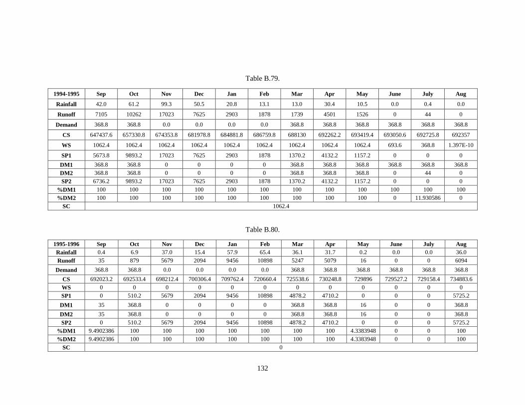
132
Table B.79.
1994-1995 Sep Oct Nov Dec Jan Feb Mar Apr May June July Aug
Rainfall 42.0 61.2 99.3 50.5 20.8 13.1 13.0 30.4 10.5 0.0 0.4 0.0
Runoff 7105 10262 17023 7625 2903 1878 1739 4501 1526 0 44 0
Demand 368.8 368.8 0.0 0.0 0.0 0.0 368.8 368.8 368.8 368.8 368.8 368.8
CS 647437.6 657330.8 674353.8 681978.8 684881.8 686759.8 688130 692262.2 693419.4 693050.6 692725.8 692357
WS 1062.4 1062.4 1062.4 1062.4 1062.4 1062.4 1062.4 1062.4 1062.4 693.6 368.8 1.397E-10
SP1 5673.8 9893.2 17023 7625 2903 1878 1370.2 4132.2 1157.2 0 0 0
DM1 368.8 368.8 0 0 0 0 368.8 368.8 368.8 368.8 368.8 368.8
DM2 368.8 368.8 0 0 0 0 368.8 368.8 368.8 0 44 0
SP2 6736.2 9893.2 17023 7625 2903 1878 1370.2 4132.2 1157.2 0 0 0
%DM1 100 100 100 100 100 100 100 100 100 100 100 100
%DM2 100 100 100 100 100 100 100 100 100 0 11.930586 0
SC 1062.4
Table B.80.
1995-1996 Sep Oct Nov Dec Jan Feb Mar Apr May June July Aug
Rainfall 0.4 6.9 37.0 15.4 57.9 65.4 36.1 31.7 0.2 0.0 0.0 36.0
Runoff 35 879 5679 2094 9456 10898 5247 5079 16 0 0 6094
Demand 368.8 368.8 0.0 0.0 0.0 0.0 368.8 368.8 368.8 368.8 368.8 368.8
CS 692023.2 692533.4 698212.4 700306.4 709762.4 720660.4 725538.6 730248.8 729896 729527.2 729158.4 734883.6
WS 0 0 0 0 0 0 0 0 0 0 0 0
SP1 0 510.2 5679 2094 9456 10898 4878.2 4710.2 0 0 0 5725.2
DM1 35 368.8 0 0 0 0 368.8 368.8 16 0 0 368.8
DM2 35 368.8 0 0 0 0 368.8 368.8 16 0 0 368.8
SP2 0 510.2 5679 2094 9456 10898 4878.2 4710.2 0 0 0 5725.2
%DM1 9.4902386 100 100 100 100 100 100 100 4.3383948 0 0 100
%DM2 9.4902386 100 100 100 100 100 100 100 4.3383948 0 0 100
SC 0
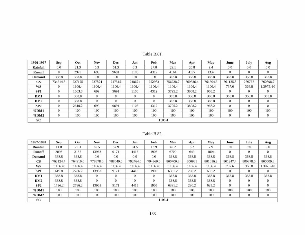
133
Table B.81.
1996-1997 Sep Oct Nov Dec Jan Feb Mar Apr May June July Aug
Rainfall 0.0 21.3 5.3 61.3 8.3 27.8 29.1 26.8 9.4 0.0 0.0 0.0
Runoff 0 2979 699 9691 1106 4312 4164 4177 1337 0 0 0
Demand 368.8 368.8 0.0 0.0 0.0 0.0 368.8 368.8 368.8 368.8 368.8 368.8
CS 734514.8 737125 737824 747515 748621 752933 756728.2 760536.4 761504.6 761135.8 760767 760398.2
WS 0 1106.4 1106.4 1106.4 1106.4 1106.4 1106.4 1106.4 1106.4 737.6 368.8 1.397E-10
SP1 0 1503.8 699 9691 1106 4312 3795.2 3808.2 968.2 0 0 0
DM1 0 368.8 0 0 0 0 368.8 368.8 368.8 368.8 368.8 368.8
DM2 0 368.8 0 0 0 0 368.8 368.8 368.8 0 0 0
SP2 0 2610.2 699 9691 1106 4312 3795.2 3808.2 968.2 0 0 0
%DM1 0 100 100 100 100 100 100 100 100 100 100 100
%DM2 0 100 100 100 100 100 100 100 100 0 0 0
SC 1106.4
Table B.82.
1997-1998 Sep Oct Nov Dec Jan Feb Mar Apr May June July Aug
Rainfall 14.0 22.3 82.5 57.9 31.5 13.9 42.2 5.2 7.9 0.0 0.0 0.0
Runoff 2095 3155 13968 9171 4415 1905 6700 649 1004 0 0 0
Demand 368.8 368.8 0.0 0.0 0.0 0.0 368.8 368.8 368.8 368.8 368.8 368.8
CS 762124.4 764910.6 778878.6 788049.6 792464.6 794369.6 800700.8 800981 801616.2 801247.4 800878.6 800509.8
WS 1106.4 1106.4 1106.4 1106.4 1106.4 1106.4 1106.4 1106.4 1106.4 737.6 368.8 1.397E-10
SP1 619.8 2786.2 13968 9171 4415 1905 6331.2 280.2 635.2 0 0 0
DM1 368.8 368.8 0 0 0 0 368.8 368.8 368.8 368.8 368.8 368.8
DM2 368.8 368.8 0 0 0 0 368.8 368.8 368.8 0 0 0
SP2 1726.2 2786.2 13968 9171 4415 1905 6331.2 280.2 635.2 0 0 0
%DM1 100 100 100 100 100 100 100 100 100 100 100 100
%DM2 100 100 100 100 100 100 100 100 100 0 0 0
SC 1106.4

134
Table B.83.
1998-1999 Sep Oct Nov Dec Jan Feb Mar Apr May June July Aug
Rainfall 0.0 1.0 31.7 86.4 102.9 30.7 31.8 39.6 0.0 0.0 0.0 0.0
Runoff 0 116 4554 14237 18114 4728 4804 6577 0 0 0 0
Demand 368.8 368.8 0.0 0.0 0.0 0.0 368.8 368.8 368.8 368.8 368.8 368.8
CS 800141 799888.2 804442.2 818679.2 836793.2 841521.2 845956.4 852164.6 851795.8 851427 851058.2 850689.4
WS 0 0 1475.2 1475.2 1475.2 1475.2 1475.2 1475.2 1106.4 737.6 368.8 1.863E-10
SP1 0 0 3078.8 14237 18114 4728 4435.2 6208.2 0 0 0 0
DM1 1.397E-10 116 0 0 0 0 368.8 368.8 368.8 368.8 368.8 368.8
DM2 0 116 0 0 0 0 368.8 368.8 0 0 0 0
SP2 0 0 4554 14237 18114 4728 4435.2 6208.2 0 0 0 0
%DM1 3.789E-11 31.453362 100 100 100 100 100 100 100 100 100 100
%DM2 0 31.453362 100 100 100 100 100 100 0 0 0 0
SC 1475.2
Table B.84.
1999-2000 Sep Oct Nov Dec Jan Feb Mar Apr May June July Aug
Rainfall 1.4 1.0 18.2 33.1 39.0 70.1 28.6 25.3 4.1 0.0 0.0 0.0
Runoff 161 116 2672 5113 5468 11137 4051 3602 524 0 0 0
Demand 368.8 368.8 0.0 0.0 0.0 0.0 368.8 368.8 368.8 368.8 368.8 368.8
CS 850481.6 850228.8 852900.8 858013.8 863481.8 874618.8 878301 881534.2 881689.4 881320.6 880951.8 880583
WS 0 0 1106.4 1106.4 1106.4 1106.4 1106.4 1106.4 1106.4 737.6 368.8 1.397E-10
SP1 0 0 1565.6 5113 5468 11137 3682.2 3233.2 155.2 0 0 0
DM1 161 116 0 0 0 0 368.8 368.8 368.8 368.8 368.8 368.8
DM2 161 116 0 0 0 0 368.8 368.8 368.8 0 0 0
SP2 0 0 2672 5113 5468 11137 3682.2 3233.2 155.2 0 0 0
%DM1 43.655098 31.453362 100 100 100 100 100 100 100 100 100 100
%DM2 43.655098 31.453362 100 100 100 100 100 100 100 0 0 0
SC 1106.4
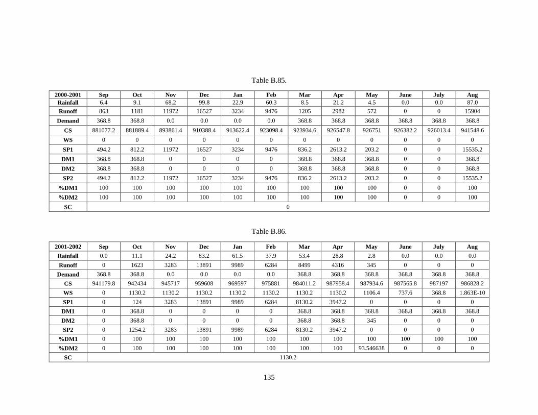
135
Table B.85.
2000-2001 Sep Oct Nov Dec Jan Feb Mar Apr May June July Aug
Rainfall 6.4 9.1 68.2 99.8 22.9 60.3 8.5 21.2 4.5 0.0 0.0 87.0
Runoff 863 1181 11972 16527 3234 9476 1205 2982 572 0 0 15904
Demand 368.8 368.8 0.0 0.0 0.0 0.0 368.8 368.8 368.8 368.8 368.8 368.8
CS 881077.2 881889.4 893861.4 910388.4 913622.4 923098.4 923934.6 926547.8 926751 926382.2 926013.4 941548.6
WS 0 0 0 0 0 0 0 0 0 0 0 0
SP1 494.2 812.2 11972 16527 3234 9476 836.2 2613.2 203.2 0 0 15535.2
DM1 368.8 368.8 0 0 0 0 368.8 368.8 368.8 0 0 368.8
DM2 368.8 368.8 0 0 0 0 368.8 368.8 368.8 0 0 368.8
SP2 494.2 812.2 11972 16527 3234 9476 836.2 2613.2 203.2 0 0 15535.2
%DM1 100 100 100 100 100 100 100 100 100 0 0 100
%DM2 100 100 100 100 100 100 100 100 100 0 0 100
SC 0
Table B.86.
2001-2002 Sep Oct Nov Dec Jan Feb Mar Apr May June July Aug
Rainfall 0.0 11.1 24.2 83.2 61.5 37.9 53.4 28.8 2.8 0.0 0.0 0.0
Runoff 0 1623 3283 13891 9989 6284 8499 4316 345 0 0 0
Demand 368.8 368.8 0.0 0.0 0.0 0.0 368.8 368.8 368.8 368.8 368.8 368.8
CS 941179.8 942434 945717 959608 969597 975881 984011.2 987958.4 987934.6 987565.8 987197 986828.2
WS 0 1130.2 1130.2 1130.2 1130.2 1130.2 1130.2 1130.2 1106.4 737.6 368.8 1.863E-10
SP1 0 124 3283 13891 9989 6284 8130.2 3947.2 0 0 0 0
DM1 0 368.8 0 0 0 0 368.8 368.8 368.8 368.8 368.8 368.8
DM2 0 368.8 0 0 0 0 368.8 368.8 345 0 0 0
SP2 0 1254.2 3283 13891 9989 6284 8130.2 3947.2 0 0 0 0
%DM1 0 100 100 100 100 100 100 100 100 100 100 100
%DM2 0 100 100 100 100 100 100 100 93.546638 0 0 0
SC 1130.2
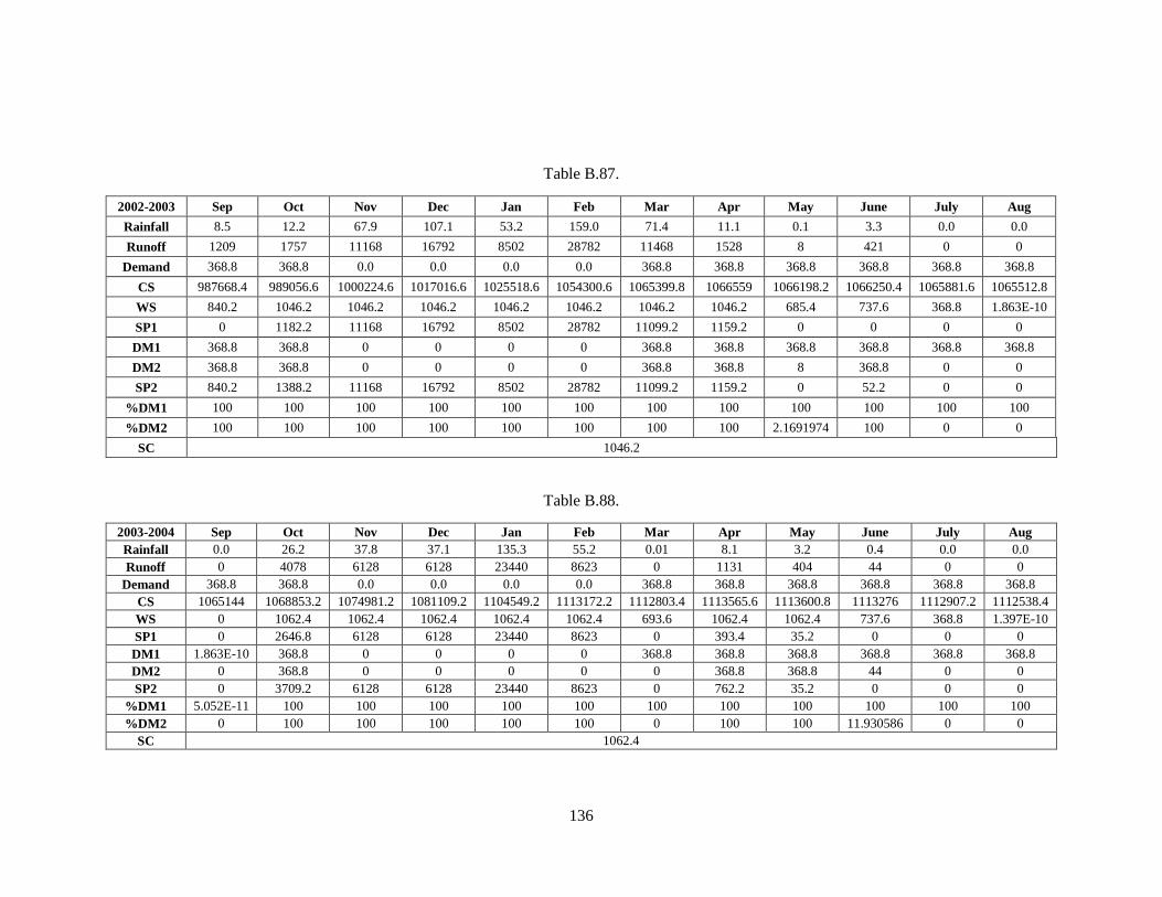
136
Table B.87.
2002-2003 Sep Oct Nov Dec Jan Feb Mar Apr May June July Aug
Rainfall 8.5 12.2 67.9 107.1 53.2 159.0 71.4 11.1 0.1 3.3 0.0 0.0
Runoff 1209 1757 11168 16792 8502 28782 11468 1528 8 421 0 0
Demand 368.8 368.8 0.0 0.0 0.0 0.0 368.8 368.8 368.8 368.8 368.8 368.8
CS 987668.4 989056.6 1000224.6 1017016.6 1025518.6 1054300.6 1065399.8 1066559 1066198.2 1066250.4 1065881.6 1065512.8
WS 840.2 1046.2 1046.2 1046.2 1046.2 1046.2 1046.2 1046.2 685.4 737.6 368.8 1.863E-10
SP1 0 1182.2 11168 16792 8502 28782 11099.2 1159.2 0 0 0 0
DM1 368.8 368.8 0 0 0 0 368.8 368.8 368.8 368.8 368.8 368.8
DM2 368.8 368.8 0 0 0 0 368.8 368.8 8 368.8 0 0
SP2 840.2 1388.2 11168 16792 8502 28782 11099.2 1159.2 0 52.2 0 0
%DM1 100 100 100 100 100 100 100 100 100 100 100 100
%DM2 100 100 100 100 100 100 100 100 2.1691974 100 0 0
SC 1046.2
Table B.88.
2003-2004 Sep Oct Nov Dec Jan Feb Mar Apr May June July Aug
Rainfall 0.0 26.2 37.8 37.1 135.3 55.2 0.01 8.1 3.2 0.4 0.0 0.0
Runoff 0 4078 6128 6128 23440 8623 0 1131 404 44 0 0
Demand 368.8 368.8 0.0 0.0 0.0 0.0 368.8 368.8 368.8 368.8 368.8 368.8
CS 1065144 1068853.2 1074981.2 1081109.2 1104549.2 1113172.2 1112803.4 1113565.6 1113600.8 1113276 1112907.2 1112538.4
WS 0 1062.4 1062.4 1062.4 1062.4 1062.4 693.6 1062.4 1062.4 737.6 368.8 1.397E-10
SP1 0 2646.8 6128 6128 23440 8623 0 393.4 35.2 0 0 0
DM1 1.863E-10 368.8 0 0 0 0 368.8 368.8 368.8 368.8 368.8 368.8
DM2 0 368.8 0 0 0 0 0 368.8 368.8 44 0 0
SP2 0 3709.2 6128 6128 23440 8623 0 762.2 35.2 0 0 0
%DM1 5.052E-11 100 100 100 100 100 100 100 100 100 100 100
%DM2 0 100 100 100 100 100 0 100 100 11.930586 0 0
SC 1062.4

137
Table B.89.
2004-2005 Sep Oct Nov Dec Jan Feb Mar Apr May June July Aug
Rainfall 0.0 32.2 46.9 51.6 36.8 40.8 28.8 27.9 1.1 1.0 0.0 0.0
Runoff 0 5389 7281 8135 5453 7008 4776 4572 116 116 0 0
Demand 368.8 368.8 0.0 0.0 0.0 0.0 368.8 368.8 368.8 368.8 368.8 368.8
CS 1112169.6 1117189.8 1124470.8 1132605.8 1138058.8 1145066.8 1149474 1153677.2 1153424.4 1153171.6 1152802.8 1152434
WS 0 1243.2 1243.2 1243.2 1243.2 1243.2 1243.2 1243.2 990.4 737.6 368.8 1.863E-10
SP1 0 3777 7281 8135 5453 7008 4407.2 4203.2 0 0 0 0
DM1 1.397E-10 368.8 0 0 0 0 368.8 368.8 368.8 368.8 368.8 368.8
DM2 0 368.8 0 0 0 0 368.8 368.8 116 116 0 0
SP2 0 5020.2 7281 8135 5453 7008 4407.2 4203.2 0 0 0 0
%DM1 3.789E-11 100 100 100 100 100 100 100 100 100 100 100
%DM2 0 100 100 100 100 100 100 100 31.453362 31.453362 0 0
SC 1243.2
Table B.90.
2005-2006 Sep Oct Nov Dec Jan Feb Mar Apr May June July Aug
Rainfall 0.0 18.5 46.3 10.7 70.6 29.4 24.6 32.6 3.7 0.0 0.01 0.0
Runoff 0 2658 7123 1439 11629 4789 3539 5284 468 0 0 0
Demand 368.8 368.8 0.0 0.0 0.0 0.0 368.8 368.8 368.8 368.8 368.8 368.8
CS 1152065.2 1154354.4 1161477.4 1162916.4 1174545.4 1179334.4 1182504.6 1187419.8 1187519 1187150.2 1186781.4 1186412.6
WS 0 1106.4 1106.4 1106.4 1106.4 1106.4 1106.4 1106.4 1106.4 737.6 368.8 1.397E-10
SP1 0 1182.8 7123 1439 11629 4789 3170.2 4915.2 99.2 0 0 0
DM1 1.863E-10 368.8 0 0 0 0 368.8 368.8 368.8 368.8 368.8 368.8
DM2 0 368.8 0 0 0 0 368.8 368.8 368.8 0 0 0
SP2 0 2289.2 7123 1439 11629 4789 3170.2 4915.2 99.2 0 0 0
%DM1 5.052E-11 100 100 100 100 100 100 100 100 100 100 100
%DM2 0 100 100 100 100 100 100 100 100 0 0 0
SC 1106.4

138
Table B.91.
2006-2007 Sep Oct Nov Dec Jan Feb Mar Apr May June July Aug
Rainfall 0.4 45.8 14.6 3.7 34.7 75.1 27.1 7.8 84.1 1.0 0.0 0.0
Runoff 43 7163 2022 456 5137 11989 4308 1035 15055 116 0 0
Demand 368.8 368.8 0.0 0.0 0.0 0.0 368.8 368.8 368.8 368.8 368.8 368.8
CS 1186086.8 1192881 1194903 1195359 1200496 1212485 1216424.2 1217090.4 1231776.6 1231523.8 1231155 1230786.2
WS 0 990.4 990.4 990.4 990.4 990.4 990.4 990.4 990.4 737.6 368.8 1.397E-10
SP1 0 5803.8 2022 456 5137 11989 3939.2 666.2 14686.2 0 0 0
DM1 43 368.8 0 0 0 0 368.8 368.8 368.8 368.8 368.8 368.8
DM2 43 368.8 0 0 0 0 368.8 368.8 368.8 116 0 0
SP2 0 6794.2 2022 456 5137 11989 3939.2 666.2 14686.2 0 0 0
%DM1 11.659436 100 100 100 100 100 100 100 100 100 100 100
%DM2 11.659436 100 100 100 100 100 100 100 100 31.453362 0 0
SC 990.4
Table B.92.
2007-2008 Sep Oct Nov Dec Jan Feb Mar Apr May June July Aug
Rainfall 0.0 0.0 33.5 40.1 15.4 31.0 7.1 1.5 3.5 0.0 0.0 0.0
Runoff 0 0 5548 6182 2245 4839 886 181 455 0 0 0
Demand 368.8 368.8 0.0 0.0 0.0 0.0 368.8 368.8 368.8 368.8 368.8 368.8
CS 1230417.4 1230048.6 1235596.6 1241778.6 1244023.6 1248862.6 1249379.8 1249192 1249278.2 1248909.4 1248540.6 1248171.8
WS 0 0 1208 1208 1208 1208 1208 1020.2 1106.4 737.6 368.8 2.329E-10
SP1 0 0 4340 6182 2245 4839 517.2 0 0 0 0 0
DM1 1.397E-10 0 0 0 0 0 368.8 368.8 368.8 368.8 368.8 368.8
DM2 0 0 0 0 0 0 368.8 181 368.8 0 0 0
SP2 0 0 5548 6182 2245 4839 517.2 0 86.2 0 0 0
%DM1 3.789E-11 0 100 100 100 100 100 100 100 100 100 100
%DM2 0 0 100 100 100 100 100 49.078091 100 0 0 0
SC 1208
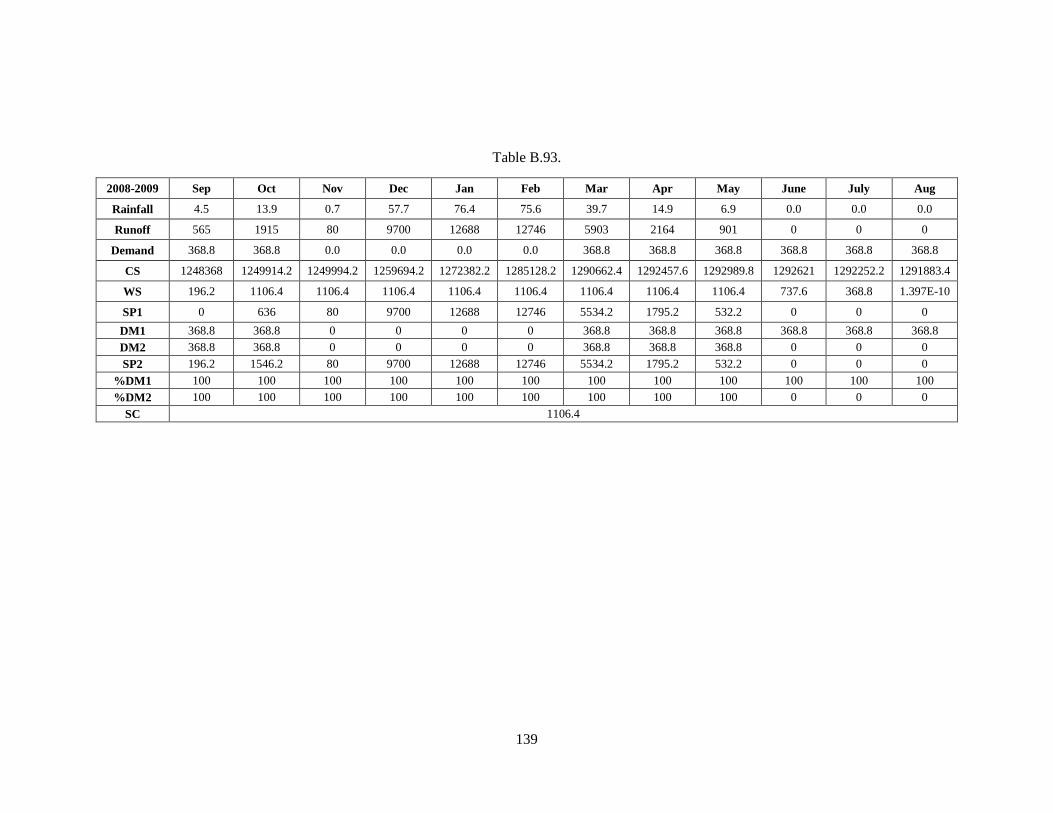
139
Table B.93.
2008-2009 Sep Oct Nov Dec Jan Feb Mar Apr May June July Aug
Rainfall 4.5 13.9 0.7 57.7 76.4 75.6 39.7 14.9 6.9 0.0 0.0 0.0
Runoff 565 1915 80 9700 12688 12746 5903 2164 901 0 0 0
Demand 368.8 368.8 0.0 0.0 0.0 0.0 368.8 368.8 368.8 368.8 368.8 368.8
CS 1248368 1249914.2 1249994.2 1259694.2 1272382.2 1285128.2 1290662.4 1292457.6 1292989.8 1292621 1292252.2 1291883.4
WS 196.2 1106.4 1106.4 1106.4 1106.4 1106.4 1106.4 1106.4 1106.4 737.6 368.8 1.397E-10
SP1 0 636 80 9700 12688 12746 5534.2 1795.2 532.2 0 0 0
DM1 368.8 368.8 0 0 0 0 368.8 368.8 368.8 368.8 368.8 368.8
DM2 368.8 368.8 0 0 0 0 368.8 368.8 368.8 0 0 0
SP2 196.2 1546.2 80 9700 12688 12746 5534.2 1795.2 532.2 0 0 0
%DM1 100 100 100 100 100 100 100 100 100 100 100 100
%DM2 100 100 100 100 100 100 100 100 100 0 0 0
SC 1106.4

140
APPENDIX C
MAPS OF METU-NCC
Figure C.1 and Figure C.2 are enlarged from Figure 3.4, in Chapter III, page 29 and
Figure 4.4 from Chapter IV, page 37 respectively.
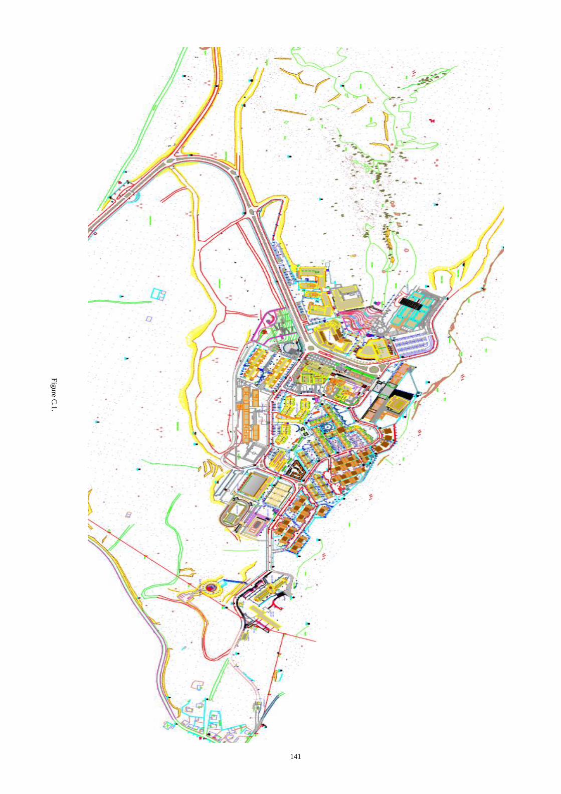
141
Fig
ure C
.1.

142
Sub
-cat
chm
ent
1
Sub
-cat
chm
ent
2
Sub
-cat
chm
ent
3
Sub
-cat
chm
ent
4
Sub
-cat
chm
ent
5
Sub
-cat
chm
ent
6
Sub
-cat
chm
ent
7
Fig
ure
C.2
.


