
Frank van den BoschYale University, spring 2017
ASTR 610 Theory of Galaxy Formation
Lecture 4: Newtonian Perturbation Theory I. Linearized Fluid Equations
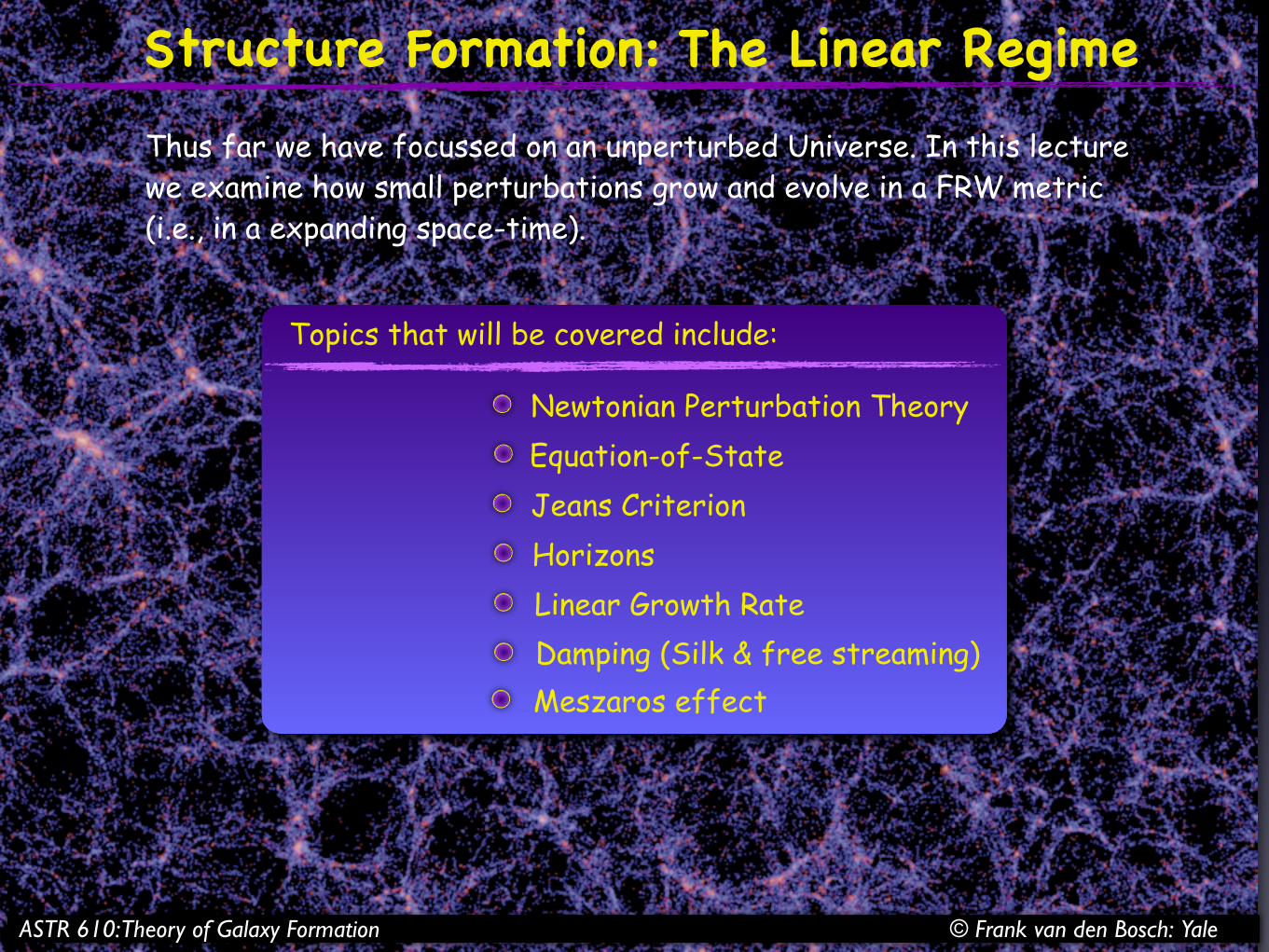
Structure Formation: The Linear RegimeThus far we have focussed on an unperturbed Universe. In this lecturewe examine how small perturbations grow and evolve in a FRW metric(i.e., in a expanding space-time).
Topics that will be covered include:
Damping (Silk & free streaming)Linear Growth RateHorizonsJeans CriterionEquation-of-StateNewtonian Perturbation Theory
Meszaros effect
ASTR 610: Theory of Galaxy Formation © Frank van den Bosch: Yale

Let be the density distribution of matter at location �(�x) �x
�(�x) =�(�x)� �
�It is useful to define the corresponding overdensity field
Note: is believed to be the outcome of some random process in the early Universe (i.e., quantum fluctuations in inflaton)
�(�x)
The Perturbed Universe: Preliminaries
Often it is very useful to describe the matter field in Fourier space:
�(�x) =�
k
��k e+i�k·�x ��k =1V
��(�x) e�i�k·�x
Here V is the volume over which the Universe is assumed to be periodic.Note: the perturbed density field can be written as a sum of plane waves of different wave numbers k (called `modes’)
ASTR 610: Theory of Galaxy Formation © Frank van den Bosch: Yale
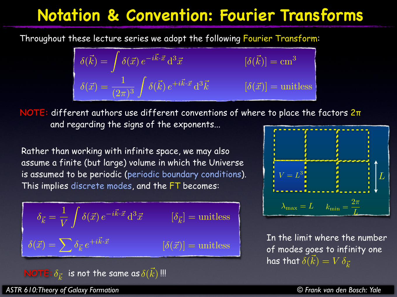
Notation & Convention: Fourier TransformsThroughout these lecture series we adopt the following Fourier Transform:
�(⇥k) =
Z�(⇥x) e�i�k·�x d3⇥x
�(⇤x) =1
(2⇥)3
Z�(⇤k) e+i�k·�x d3⇤k [�(⇥x)] = unitless
[�(⇥k)] = cm3
NOTE: different authors use different conventions of where to place the factors 2π and regarding the signs of the exponents...
Rather than working with infinite space, we may alsoassume a finite (but large) volume in which the Universeis assumed to be periodic (periodic boundary conditions).This implies discrete modes, and the FT becomes:
LV = L3
�max
= L kmin =2�
L
�(⇥x) =X
��k e+i�k·�x
��k =1
V
Z�(⇥x) e�i�k·�x d3⇥x
[�(⇥x)] = unitless
[��k] = unitless
In the limit where the number of modes goes to infinity one has that �(⇥k) = V ��k
NOTE: is not the same as !!! ��k �(⇥k)
ASTR 610: Theory of Galaxy Formation © Frank van den Bosch: Yale
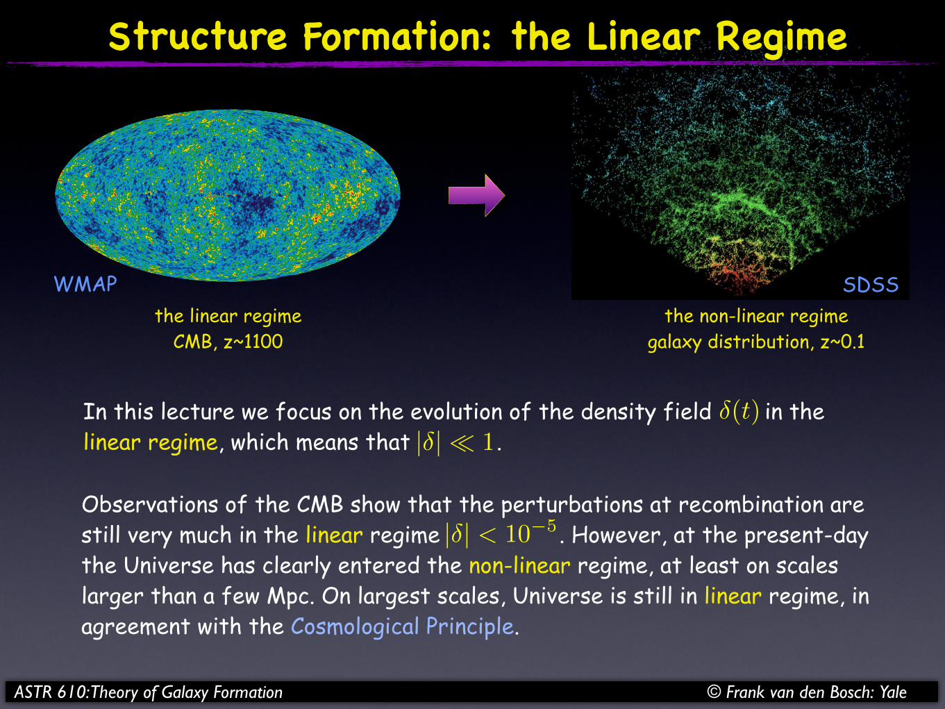
Structure Formation: the Linear Regime
�(t)In this lecture we focus on the evolution of the density field in the linear regime, which means that . |�| � 1
Observations of the CMB show that the perturbations at recombination arestill very much in the linear regime . However, at the present-daythe Universe has clearly entered the non-linear regime, at least on scaleslarger than a few Mpc. On largest scales, Universe is still in linear regime, inagreement with the Cosmological Principle.
|�| < 10�5
the linear regimeCMB, z~1100
the non-linear regimegalaxy distribution, z~0.1
WMAP SDSS
ASTR 610: Theory of Galaxy Formation © Frank van den Bosch: Yale
The Fluid Description
�(t)QUESTION: what equations describe the evolution of ?
Before recombination: photon & baryons are a tightly coupled fluid
After recombination: photons are decoupled from baryonsbaryons behave as an `ideal gas’ (i.e. a fluid)
Throughout: dark matter is (assumed to be) a collisionless fluid
ANSWER: it seems we can describe using fluid equations...�(t)
ASTR 610: Theory of Galaxy Formation © Frank van den Bosch: Yale

The Fluid DescriptionQUESTION: when is a fluid description adequate?
ANSWER: when frequent collisions can establish local thermal equilibrium, i.e., when the mean free path is much smaller than scales of interest (baryons).
for a collisionless system, as long as the velocity dispersion of the particles is sufficiently small that particle diffusion can be neglected on the scale of interest....
NOTE: As we will see, Cold Dark Matter (CDM) can be described as fluid with zero pressure (on all scales of interest to us). However, in the case of Hot Dark Matter (HDM) or Warm Dark Matter (WDM), the non-zero peculiar velocities of the dark matter particles causes free-streaming damping on small scales. On those scales the fluid description brakes down, and one has to resort to the (collisionless) Boltzmann equation.
ASTR 610: Theory of Galaxy Formation © Frank van den Bosch: Yale

Fluid EquationsLet , , and describe the density, velocity, and pressure ofa fluid at location at time , with the corresponding gravitational potential.
�(⇥x, t) P (�x, t)�u(�x, t)�(⇥x, t)�x t
The time evolution of this fluid is given by the continuity equation (describing mass conservation), the Euler equations (the eqs. of motion), and the Poisson equation (describing the gravitational field:
D⇤u
Dt= �rrP
��rr⇥
D�
Dt+ ��r · ⇥u = 0
r2r⇤ = 4�G⇥
continuity equation
Euler equations
Poisson equation
is the Lagrangian (or `convective’) derivative, which means the derivative wrt a moving fluid element (as opposed to the Eulerian derivatives wrt some fixed grid point...).
D
Dt=
�
�t+ ⇥u ·�rNOTE:
NOTE: The continuity & Euler eqs are moment eqs of the Boltzmann eq.
ASTR 610: Theory of Galaxy Formation © Frank van den Bosch: Yale

�u = r = a�x+ a�x ⌘ a�x+ �v
�
�t⇥ �
�t� a
a⇥x ·⇤
rr
! 1
ar
x
=1
ar
Eulerian time-derivative depends on H(t)
�v = peculiar velocity
�xit is understood that gradient is wrt
Fluid Equations
the halo bias function
D⇤u
Dt= �rrP
��rr⇥
D�
Dt+ ��r · ⇥u = 0
r2r⇤ = 4�G⇥
continuity equation
Euler equations
Poisson equation
This is a set of 5 equations (3 Euler eqs + continuity + Poisson) for 6 unknowns (�, u
x
, uy
, uz
, P,⇥)
In order to close the set, we require an additionalequation, which is the equation of state (EoS)
Because of expansion, it is best to use comoving coordinates, , where �r = a(t) �x�x
Before we address this EoS, we first rewrite these fluid equations in a different form, more suited to describe perturbations in an expanding space....
at fixed xat fixed r
ASTR 610: Theory of Galaxy Formation © Frank van den Bosch: Yale
what follows is only valid for a non-relativistic fluidFluid Equations
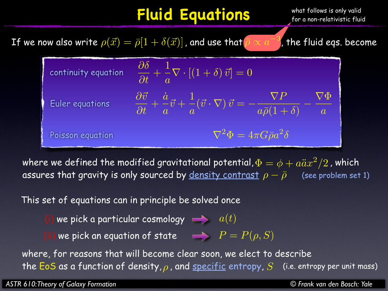
If we now also write , and use that , the fluid eqs. become⇥(⇤x) = ⇥[1 + �(⇤x)] � / a�3
⇥�
⇥t+
1
a� · [(1 + �)⇤v] = 0
r2� = 4⇥G⇤a2�
continuity equation
Euler equations
Poisson equation
⇤⌅v
⇤t+
a
a⌅v +
1
a(⌅v ·⇥)⌅v = � ⇥P
a⇥(1 + �)� ⇥�
a
� = �+ aax2/2where we defined the modified gravitational potential, , whichassures that gravity is only sourced by density contrast ⇢� ⇢ (see problem set 1)
This set of equations can in principle be solved once
(i) we pick a particular cosmology
(ii) we pick an equation of state P = P (�, S)
a(t)
where, for reasons that will become clear soon, we elect to describe the EoS as a function of density, , and specific entropy, S⇢ (i.e. entropy per unit mass)
ASTR 610: Theory of Galaxy Formation © Frank van den Bosch: Yale
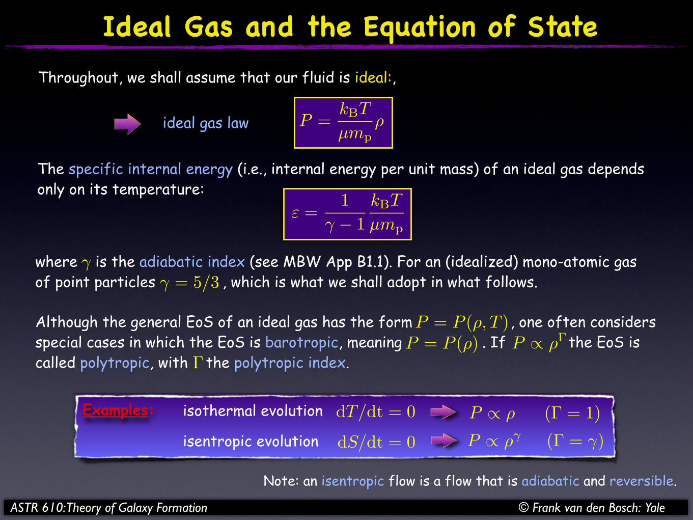
Ideal Gas and the Equation of StateThroughout, we shall assume that our fluid is ideal:,
P =kBT
µmp�ideal gas law
The specific internal energy (i.e., internal energy per unit mass) of an ideal gas dependsonly on its temperature:
� =1
� � 1kBT
µmp
where is the adiabatic index (see MBW App B1.1). For an (idealized) mono-atomic gasof point particles , which is what we shall adopt in what follows.
�� = 5/3
Although the general EoS of an ideal gas has the form , one often considersspecial cases in which the EoS is barotropic, meaning . If the EoS iscalled polytropic, with the polytropic index.
P = P (�)P = P (�, T )
P � ��
�
Examples: isothermal evolution
isentropic evolution
dT/dt = 0
dS/dt = 0 P � �� (� = �)P � � (� = 1)
Note: an isentropic flow is a flow that is adiabatic and reversible.
ASTR 610: Theory of Galaxy Formation © Frank van den Bosch: Yale

Closing the set of Fluid EquationsRecall that the EoS is needed to close the set of equations (unless the fluid ispressureless...).
TdS
dt=
dQ
dt=H� C
�
Here and are the heating and cooling rates per unit volume, respectively.H C
dS = dQ/T
P = P (�, T ) P = P (�, S)In the case of a barotropic EoS, the set of fluid equations is closed. However, in the more general case where , or equivalently, , we have introduced a new variable ( or ), and thus also require a new equation...T S
This is provided by the 2nd law of thermodynamics:where is the amount of energy added to the fluid per unit mass.dQ
For most of what follows, we assume that the evolution is adiabatic, whichimplies that . dS/dt = 0
As we shall see throughout this course, and are determined by a variety ofphysical processes (see chapter 8 of MBW) and can be calculated...
H C
ASTR 610: Theory of Galaxy Formation © Frank van den Bosch: Yale
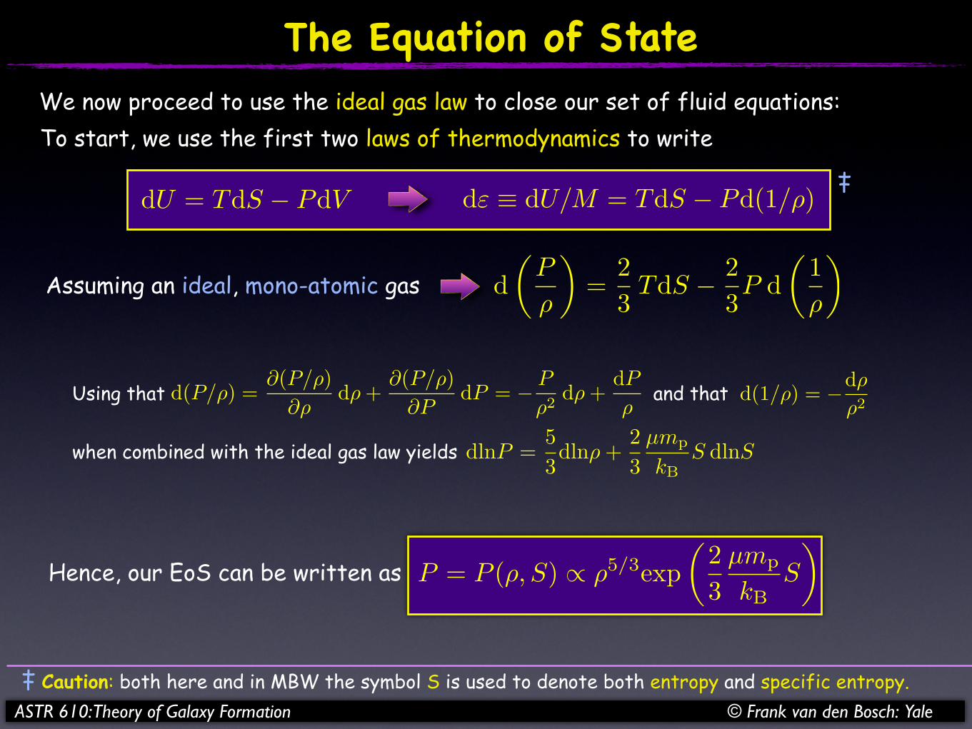
The Equation of State
Caution: both here and in MBW the symbol S is used to denote both entropy and specific entropy.
We now proceed to use the ideal gas law to close our set of fluid equations:To start, we use the first two laws of thermodynamics to write
‡
‡dU = TdS � PdV d� � dU/M = TdS � Pd(1/�)
Assuming an ideal, mono-atomic gas d�
P
�
�=
23
TdS � 23P d
�1�
�
d(P/�) =�(P/�)
��d� +
�(P/�)�P
dP = � P
�2d� +
dP
�Using that and that d(1/�) = �d�
�2
dlnP =53dln� +
23
µmp
kBS dlnSwhen combined with the ideal gas law yields
Hence, our EoS can be written as P = P (�, S) � �5/3exp�
23
µmp
kBS
�
ASTR 610: Theory of Galaxy Formation © Frank van den Bosch: Yale
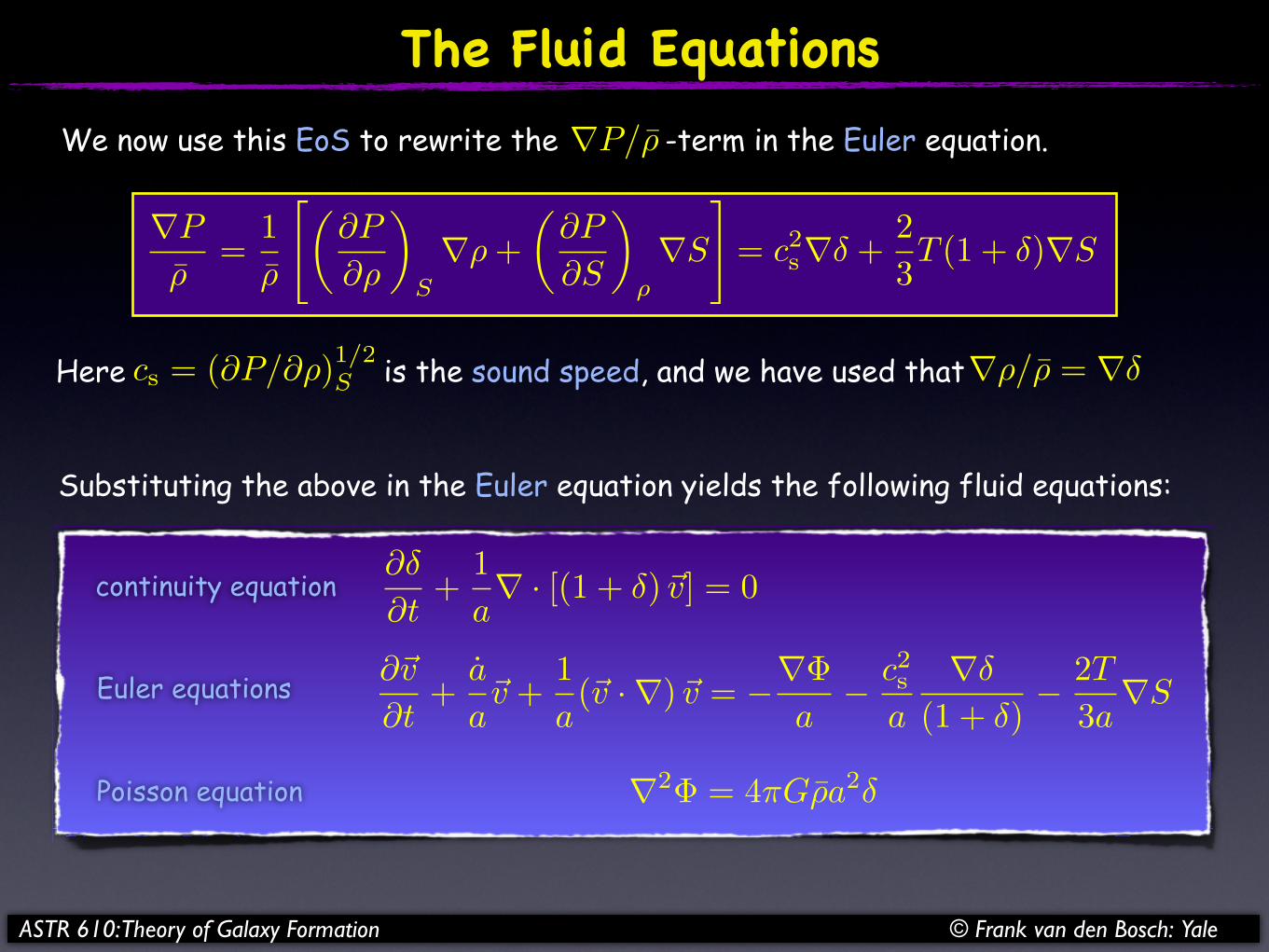
The Fluid EquationsWe now use this EoS to rewrite the -term in the Euler equation.�P/�
�P
�=
1�
���P
��
�
S
�� +�
�P
�S
�
�
�S
�= c2
s�� +23T (1 + �)�S
cs = (�P/��)1/2SHere is the sound speed, and we have used that��/� = ��
Substituting the above in the Euler equation yields the following fluid equations:
⇥�
⇥t+
1
a� · [(1 + �)⇤v] = 0
r2� = 4⇥G⇤a2�
continuity equation
Euler equations
Poisson equation
��v
�t+
a
a�v +
1a(�v ·�)�v = ���
a� c2
s
a
��
(1 + �)� 2T
3a�S
ASTR 610: Theory of Galaxy Formation © Frank van den Bosch: Yale

Linearizing the Fluid EquationsThe next step is to linearize the fluid equations: Using that both and are small,we can neglect all higher order terms (those with , , or ).
� vv2�2 � v
T = T + �TIf we write and also igore higher-order terms containing thesmall temperature perturbation , the fluid equations simplify to �T
Differentiating the continuity eq. wrt and using the Euler & Poisson eqs yields:t
�2�
�t2+ 2
a
a
��
�t= 4�G�� +
c2s
a2�2� +
23
T
a2�2S
This `master equation’ describes the evolution of the density perturbationsin the linear regime ( ), but only for a non-relativistic fluid !!!|�|� 1
ASTR 610: Theory of Galaxy Formation © Frank van den Bosch: Yale
continuity equation
Euler equations��v
�t+
a
a�v = ���
a� c2
s
a�� � 2T
3a�S
��
�t+
1a� · �v = 0
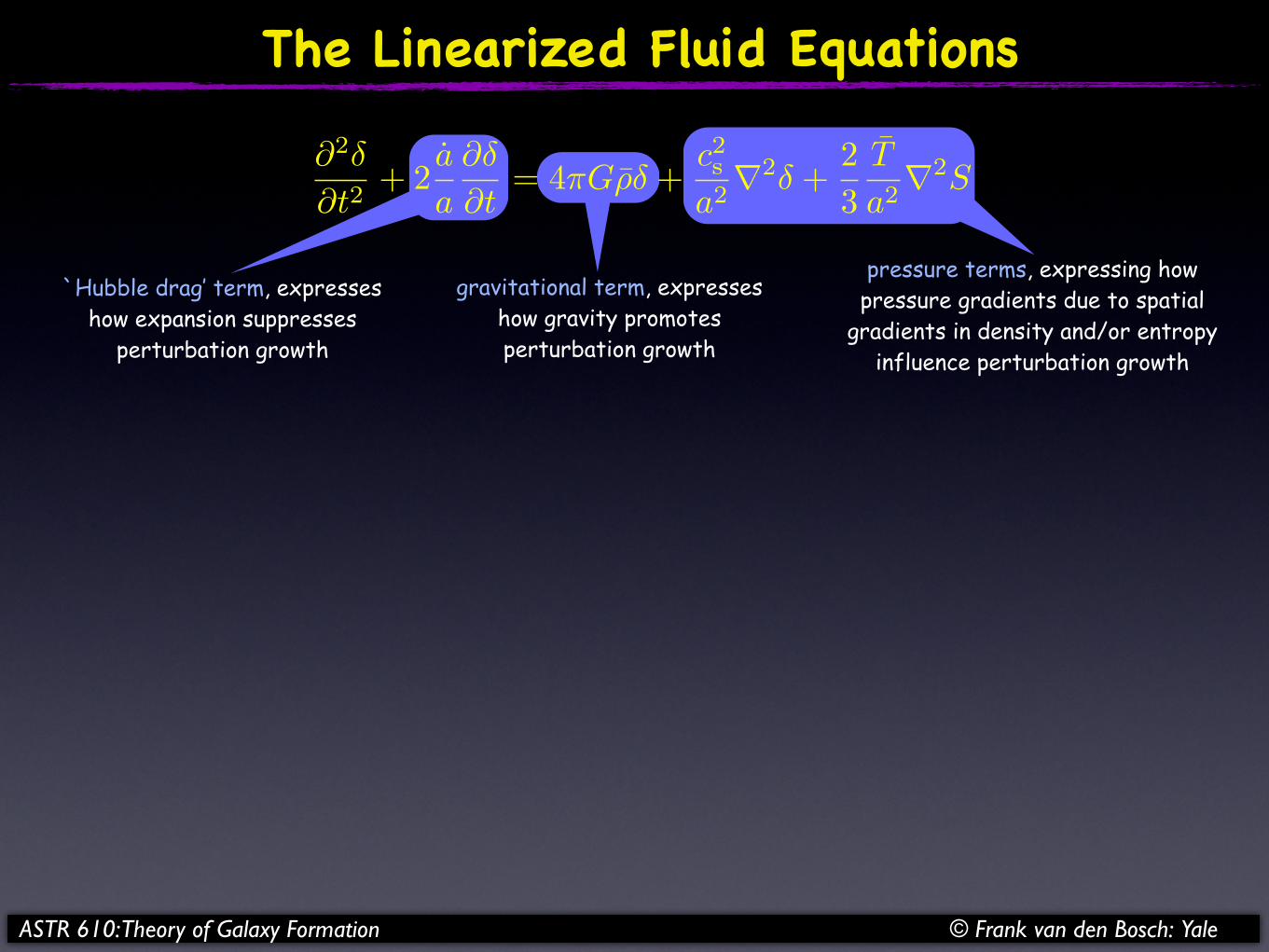
gravitational term, expresses how gravity promotes perturbation growth
The Linearized Fluid Equations
`Hubble drag’ term, expresses how expansion suppresses
perturbation growth
pressure terms, expressing how pressure gradients due to spatial
gradients in density and/or entropy influence perturbation growth
�2�
�t2+ 2
a
a
��
�t= 4�G�� +
c2s
a2�2� +
23
T
a2�2S
ASTR 610: Theory of Galaxy Formation © Frank van den Bosch: Yale
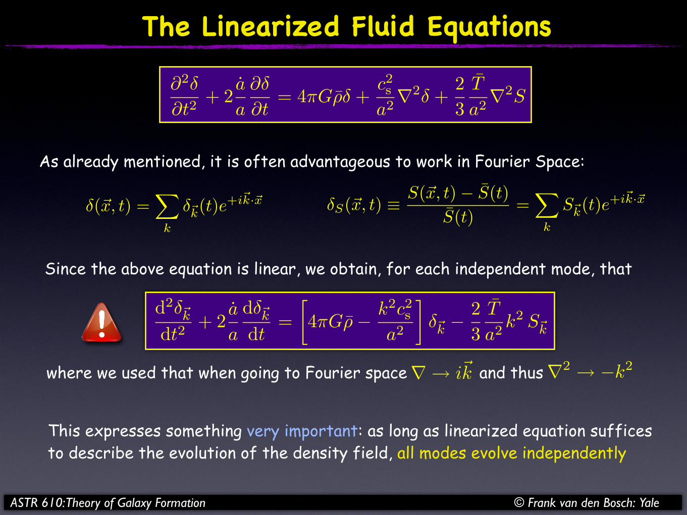
The Linearized Fluid Equations
�2�
�t2+ 2
a
a
��
�t= 4�G�� +
c2s
a2�2� +
23
T
a2�2S
As already mentioned, it is often advantageous to work in Fourier Space:
Since the above equation is linear, we obtain, for each independent mode, that
where we used that when going to Fourier space and thus� � i�k �2 � �k2
d2��k
dt2+ 2
a
a
d��k
dt=
�4�G�� k2c2
s
a2
���k �
23
T
a2k2 S�k
This expresses something very important: as long as linearized equation sufficesto describe the evolution of the density field, all modes evolve independently
�S(�x, t) � S(�x, t)� S(t)S(t)
=�
k
S�k(t)e+i�k·�x�(�x, t) =�
k
��k(t)e+i�k·�x
ASTR 610: Theory of Galaxy Formation © Frank van den Bosch: Yale
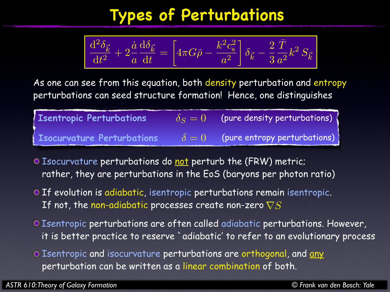
Types of Perturbationsd2��k
dt2+ 2
a
a
d��k
dt=
�4�G�� k2c2
s
a2
���k �
23
T
a2k2 S�k
As one can see from this equation, both density perturbation and entropy perturbations can seed structure formation! Hence, one distinguishes
Isocurvature perturbations do not perturb the (FRW) metric; rather, they are perturbations in the EoS (baryons per photon ratio)
If evolution is adiabatic, isentropic perturbations remain isentropic.If not, the non-adiabatic processes create non-zero�S
Isentropic and isocurvature perturbations are orthogonal, and any perturbation can be written as a linear combination of both.
Isentropic Perturbations
Isocurvature Perturbations � = 0
�S = 0 (pure density perturbations)
(pure entropy perturbations)
ASTR 610: Theory of Galaxy Formation © Frank van den Bosch: Yale
Isentropic perturbations are often called adiabatic perturbations. However,it is better practice to reserve `adiabatic’ to refer to an evolutionary process
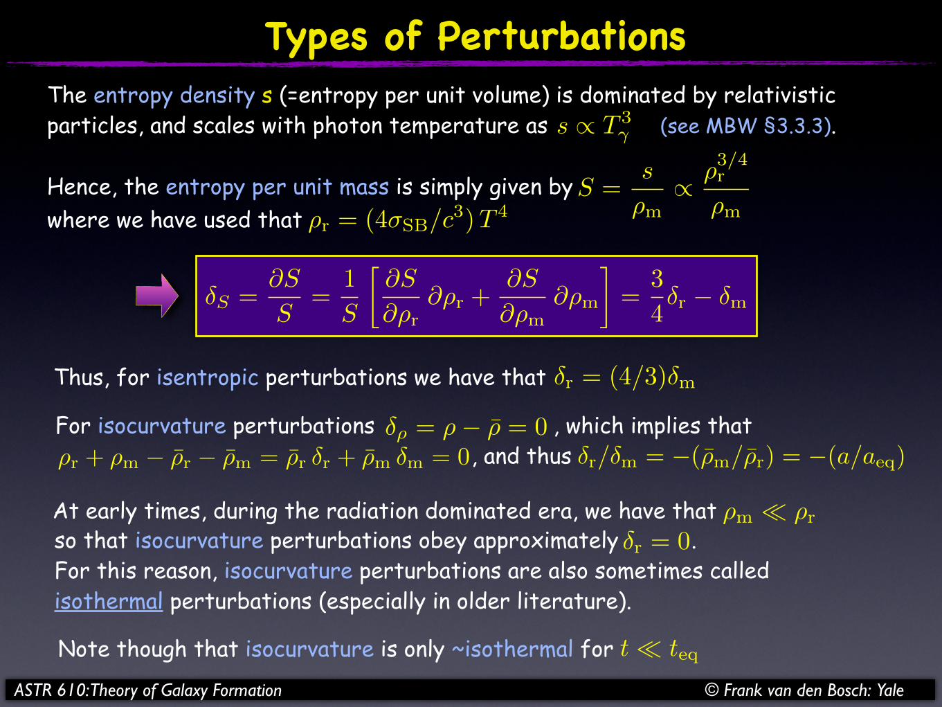
Types of PerturbationsThe entropy density s (=entropy per unit volume) is dominated by relativistic particles, and scales with photon temperature as (see MBW §3.3.3).s / T 3
�
Hence, the entropy per unit mass is simply given byS =s
�m/ �3/4r
�mwhere we have used that �r = (4⇥SB/c3)T 4
�S =⇤S
S=
1
S
⇤S
⇤⇥r⇤⇥r +
⇤S
⇤⇥m⇤⇥m
�=
3
4�r � �m
Thus, for isentropic perturbations we have that �r = (4/3)�m
At early times, during the radiation dominated era, we have that ⇢m ⌧ ⇢rso that isocurvature perturbations obey approximately . For this reason, isocurvature perturbations are also sometimes called isothermal perturbations (especially in older literature).
�r = 0
Note though that isocurvature is only ~isothermal for t ⌧ teq
ASTR 610: Theory of Galaxy Formation © Frank van den Bosch: Yale
For isocurvature perturbations , which implies that , and thus
�⇢ = ⇢� ⇢ = 0�r + �m � �r � �m = �r �r + �m �m = 0 �r/�m = �(�m/�r) = �(a/aeq)
Different Matter ComponentsThe matter perturbations that we are describing consist of both baryonsand dark matter (assumed to be collisionless).
In what follows we will first treat these separately.
We start by considering a Universe without dark matter (only baryons + radiation).
Next we considering a Universe without baryons (only dark matter + radiation).
We end with discussing a more realistic Universe (radiation + baryons + dark matter)
ASTR 610: Theory of Galaxy Formation © Frank van den Bosch: Yale


