
Astro 4PTLecture Notes Set 1
Wayne Hu

References• Relativistic Cosmological Perturbation Theory
Inflation
Dark Energy
Modified Gravity
Cosmic Microwave Background
Large Scale Structure
• Bardeen (1980), PRD 22 1882
• Kodama & Sasaki (1984), Prog. Th. Phys. Supp., 78, 1
• Mukhanov, Feldman, Brandenberger (1992), Phys. Reports, 215,203
• Malik & Wands (2009), Phys. Reports, 475, 1

Covariant Perturbation Theory• Covariant = takes same form in all coordinate systems
• Invariant = takes the same value in all coordinate systems
• Fundamental equations: Einstein equations, covariant conservationof stress-energy tensor:
Gµν = 8πGTµν
∇µTµν = 0
• Preserve general covariance by keeping all free variables: 10 foreach symmetric 4×4 tensor
1 2 3 45 6 7
8 910

Metric Tensor• Useful to think in a 3 + 1 language since there are preferred spatial
surfaces where the stress tensor is nearly homogeneous
• In general this is an Arnowitt-Deser-Misner (ADM) split
• Specialize to the case of a nearly FRW metric
g00 = −a2, gij = a2γij .
where the “0” component is conformal time η = dt/a and γij is aspatial metric of constant curvature K = H2
0 (Ωtot − 1).
(3)R =6K
a2

Metric Tensor• First define the slicing (lapse function A, shift function Bi)
g00 = −a−2(1− 2A) ,
g0i = −a−2Bi ,
A defines the lapse of proper time between 3-surfaces whereas Bi
defines the threading or relationship between the 3-coordinates ofthe surfaces
• This absorbs 1+3=4 free variables in the metric, remaining 6 is inthe spatial surfaces which we parameterize as
gij = a−2(γij − 2HLγij − 2H ij
T ) .
here (1) HL a perturbation to the spatial curvature; (5) H ijT a
trace-free distortion to spatial metric (which also can perturb thecurvature)

Curvature Perturbation• Curvature perturbation on the 3D slice
δ[(3)R] = − 4
a2(∇2 + 3K
)HL +
2
a2∇i∇jH
ijT
• Note that we will often loosely refer to HL as the “curvatureperturbation”
• We will see that many representations have HT = 0
• It is easier to work with a dimensionless quantity
• First example of a 3-scalar - SVT decomposition
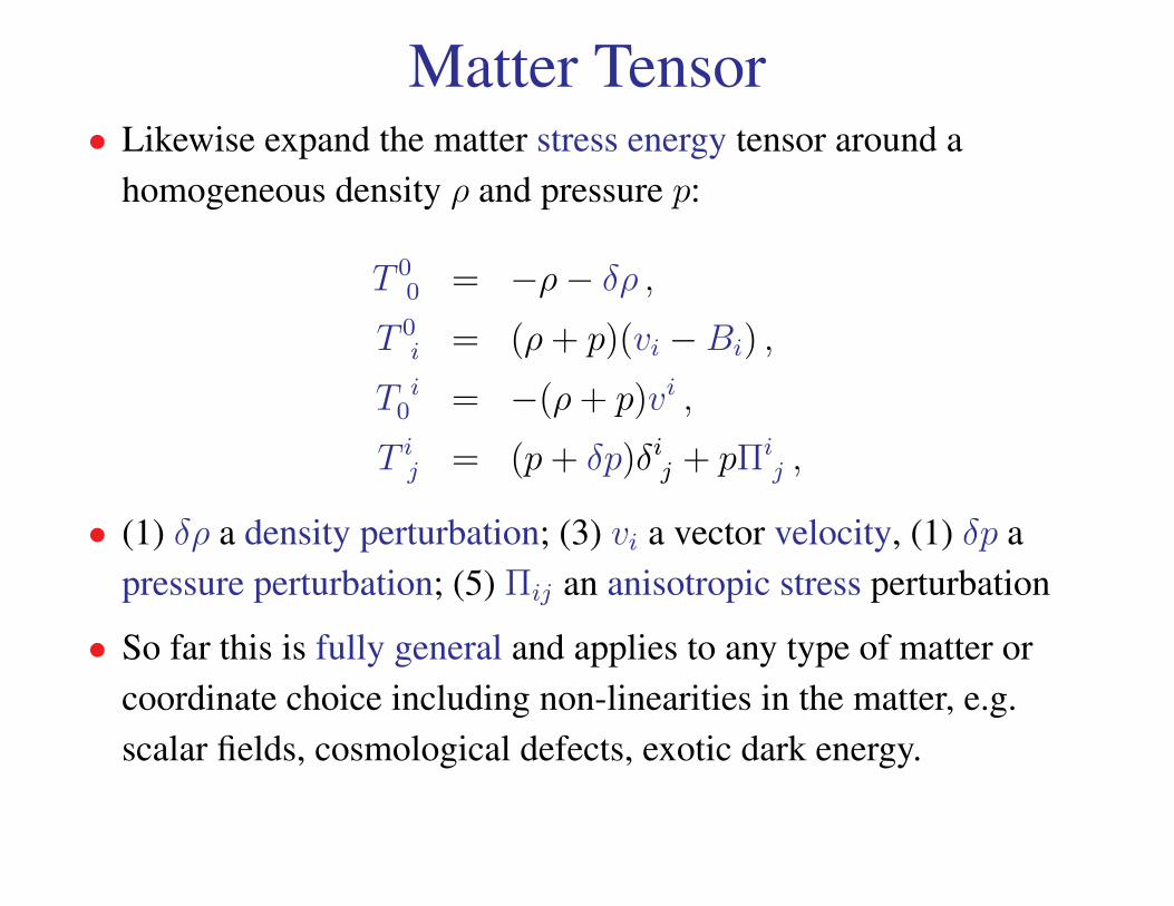
Matter Tensor• Likewise expand the matter stress energy tensor around a
homogeneous density ρ and pressure p:
T 00 = −ρ− δρ ,
T 0i = (ρ+ p)(vi −Bi) ,
T i0 = −(ρ+ p)vi ,
T ij = (p+ δp)δij + pΠij ,
• (1) δρ a density perturbation; (3) vi a vector velocity, (1) δp apressure perturbation; (5) Πij an anisotropic stress perturbation
• So far this is fully general and applies to any type of matter orcoordinate choice including non-linearities in the matter, e.g.scalar fields, cosmological defects, exotic dark energy.

Counting Variables
20 Variables (10 metric; 10 matter)
−10 Einstein equations
−4 Conservation equations
+4 Bianchi identities
−4 Gauge (coordinate choice 1 time, 3 space)
——
6 Free Variables
• Without loss of generality these can be taken to be the 6components of the matter stress tensor
• For the background, specify p(a) or equivalentlyw(a) ≡ p(a)/ρ(a) the equation of state parameter.

Homogeneous Einstein Equations• Einstein (Friedmann) equations:(
1
a
da
dt
)2
= −Ka2
+8πG
3ρ [=
(1
a
a
a
)2
]
1
a
d2a
dt2= −4πG
3(ρ+ 3p) [=
1
a2d
dη
a
a]
so that w ≡ p/ρ < −1/3 for acceleration
• Conservation equation∇µTµν = 0 implies
ρ
ρ= −3(1 + w)
a
a
overdots are conformal time but equally true with coordinate time

Homogeneous Einstein Equations• Counting exercise:
20 Variables (10 metric; 10 matter)
−17 Homogeneity and Isotropy
−2 Einstein equations
−1 Conservation equations
+1 Bianchi identities
——
1 Free Variables
without loss of generality choose ratio of homogeneous & isotropiccomponent of the stress tensor to the density w(a) = p(a)/ρ(a).

Acceleration Implies Negative Pressure• Role of stresses in the background cosmology
• Homogeneous Einstein equations Gµν = 8πGTµν imply the twoFriedmann equations (flat universe, or associating curvatureρK = −3K/8πGa2)(
1
a
da
dt
)2
=8πG
3ρ
1
a
d2a
dt2= −4πG
3(ρ+ 3p)
so that the total equation of state w ≡ p/ρ < −1/3 for acceleration
• Conservation equation∇µTµν = 0 implies
ρ
ρ= −3(1 + w)
a
a
so that ρ must scale more slowly than a−2

Scalar, Vector, Tensor• In linear perturbation theory, perturbations may be separated by
their transformation properties under 3D rotation and translation.
• The eigenfunctions of the Laplacian operator form a complete set
∇2Q(0) = −k2Q(0) S ,
∇2Q(±1)i = −k2Q(±1)
i V ,
∇2Q(±2)ij = −k2Q(±2)
ij T ,
• Vector and tensor modes satisfy divergence-free andtransverse-traceless conditions
∇iQ(±1)i = 0
∇iQ(±2)ij = 0
γijQ(±2)ij = 0
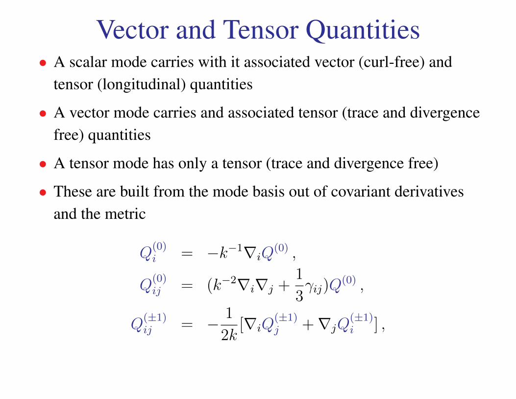
Vector and Tensor Quantities• A scalar mode carries with it associated vector (curl-free) and
tensor (longitudinal) quantities
• A vector mode carries and associated tensor (trace and divergencefree) quantities
• A tensor mode has only a tensor (trace and divergence free)
• These are built from the mode basis out of covariant derivativesand the metric
Q(0)i = −k−1∇iQ
(0) ,
Q(0)ij = (k−2∇i∇j +
1
3γij)Q
(0) ,
Q(±1)ij = − 1
2k[∇iQ
(±1)j +∇jQ
(±1)i ] ,

Perturbation k-Modes• For the kth eigenmode, the scalar components become
A(x) = A(k)Q(0) , HL(x) = HL(k)Q(0) ,
δρ(x) = δρ(k)Q(0) , δp(x) = δp(k)Q(0) ,
the vectors components become
Bi(x) =1∑
m=−1
B(m)(k)Q(m)i , vi(x) =
1∑m=−1
v(m)(k)Q(m)i ,
and the tensors components
HT ij(x) =2∑
m=−2
H(m)T (k)Q
(m)ij , Πij(x) =
2∑m=−2
Π(m)(k)Q(m)ij ,
• Note that the curvature perturbation only involves scalars
δ[(3)R] =4
a2(k2 − 3K)(H
(0)L +
1
3H
(0)T )Q(0)

Spatially Flat Case• For a spatially flat background metric, harmonics are related to
plane waves:
Q(0) = exp(ik · x)
Q(±1)i =
−i√2
(e1 ± ie2)iexp(ik · x)
Q(±2)ij = −
√3
8(e1 ± ie2)i(e1 ± ie2)jexp(ik · x)
where e3 ‖ k. Chosen as spin states, c.f. polarization.
• For vectors, the harmonic points in a direction orthogonal to k
suitable for the vortical component of a vector

Spatially Flat Case• Tensor harmonics are the transverse traceless gauge representation
• Tensor amplitude related to the more traditional
h+[(e1)i(e1)j − (e2)i(e2)j] , h×[(e1)i(e2)j + (e2)i(e1)j]
as
h+ ± ih× = −√
6H(∓2)T
• H(±2)T proportional to the right and left circularly polarized
amplitudes of gravitational waves with a normalization that isconvenient to match the scalar and vector definitions

Covariant Scalar Equations• DOF counting exercise
8 Variables (4 metric; 4 matter)
−4 Einstein equations
−2 Conservation equations
+2 Bianchi identities
−2 Gauge (coordinate choice 1 time, 1 space)
——
2 Free Variables
without loss of generality choose scalar components of the stresstensor δp, Π .

Covariant Scalar Equations• Einstein equations (suppressing 0) superscripts
(k2 − 3K)[HL +1
3HT ]− 3(
a
a)2A+ 3
a
aHL +
a
akB =
= 4πGa2δρ , 00 Poisson Equation
k2(A+HL +1
3HT ) +
(d
dη+ 2
a
a
)(kB − HT )
= −8πGa2pΠ , ij Anisotropy Equationa
aA− HL −
1
3HT −
K
k2(kB − HT )
= 4πGa2(ρ+ p)(v −B)/k , 0i Momentum Equation[2a
a− 2
(a
a
)2
+a
a
d
dη− k2
3
]A−
[d
dη+a
a
](HL +
1
3kB)
= 4πGa2(δp+1
3δρ) , ii Acceleration Equation

Covariant Scalar Equations• Conservation equations: continuity and Navier Stokes[
d
dη+ 3
a
a
]δρ+ 3
a
aδp = −(ρ+ p)(kv + 3HL) ,[
d
dη+ 4
a
a
] [(ρ+ p)
(v −B)
k
]= δp− 2
3(1− 3
K
k2)pΠ + (ρ+ p)A ,
• Equations are not independent since∇µGµν = 0 via the Bianchi
identities.
• Related to the ability to choose a coordinate system or “gauge” torepresent the perturbations.

Covariant Vector Equations• Einstein equations
(1− 2K/k2)(kB(±1) − H(±1)T )
= 16πGa2(ρ+ p)(v(±1) −B(±1))/k ,[d
dη+ 2
a
a
](kB(±1) − H(±1)
T )
= −8πGa2pΠ(±1) .
• Conservation Equations[d
dη+ 4
a
a
][(ρ+ p)(v(±1) −B(±1))/k]
= −1
2(1− 2K/k2)pΠ(±1) ,
• Gravity provides no source to vorticity→ decay

Covariant Vector Equations• DOF counting exercise
8 Variables (4 metric; 4 matter)
−4 Einstein equations
−2 Conservation equations
+2 Bianchi identities
−2 Gauge (coordinate choice 1 time, 1 space)
——
2 Free Variables
without loss of generality choose vector components of the stresstensor Π(±1).
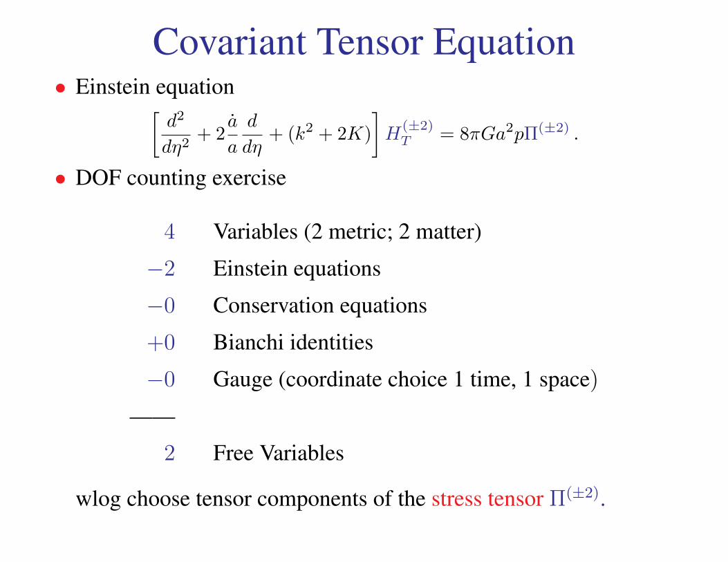
Covariant Tensor Equation• Einstein equation[
d2
dη2+ 2
a
a
d
dη+ (k2 + 2K)
]H
(±2)T = 8πGa2pΠ(±2) .
• DOF counting exercise
4 Variables (2 metric; 2 matter)
−2 Einstein equations
−0 Conservation equations
+0 Bianchi identities
−0 Gauge (coordinate choice 1 time, 1 space)
——
2 Free Variables
wlog choose tensor components of the stress tensor Π(±2).

Arbitrary Dark Components• Total stress energy tensor can be broken up into individual pieces
• Dark components interact only through gravity and so satisfyseparate conservation equations
• Einstein equation source remains the sum of components.
• To specify an arbitrary dark component, give the behavior of thestress tensor: 6 components: δp, Π(i), where i = −2, ..., 2.
• Many types of dark components (dark matter, scalar fields,massive neutrinos,..) have simple forms for their stress tensor interms of the energy density, i.e. described by equations of state.
• An equation of state for the background w = p/ρ is not sufficientto determine the behavior of the perturbations.

Separate Universes• Geometry of the gauge or time slicing and spatial threading
• For perturbations larger than the horizon, a local observer shouldjust see a different (separate) FRW universe
• Scalar equations should be equivalent to an appropriatelyremapped Friedmann equation
• Unit normal vector Nµ to constant time hypersurfacesNµdx
µ = N0dη, NµNµ = −1, to linear order in metric
N0 = −a(1 +AQ), Ni = 0
N0 = a−1(1−AQ), N i = −BQi
• Expansion of spatial volume per proper time is given by4-divergence
∇µNµ ≡ θ = 3H(1−AQ) +k
aBQ+
3
aHLQ

Shear and Acceleration• Other pieces of ∇νNµ give the vorticity, shear and acceleration
∇νNµ ≡ ωµν + σµν +1
3θPµν − aµNν
with
Pµν = gµν +NµNν
ωµν = P αµ P β
ν (∇βNα −∇αNβ)
σµν =1
2P αµ P β
ν (∇βNα +∇αNβ)− 1
3θPµν
aµ = (∇αNµ)Nα
projection PµνNν = 0, trace free antisymmetric vorticity,symmetric shear and acceleration
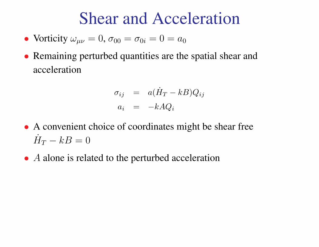
Shear and Acceleration• Vorticity ωµν = 0, σ00 = σ0i = 0 = a0
• Remaining perturbed quantities are the spatial shear andacceleration
σij = a(HT − kB)Qij
ai = −kAQi
• A convenient choice of coordinates might be shear freeHT − kB = 0
• A alone is related to the perturbed acceleration

Separate Universes• So the e-foldings of the expansion are given by dτ = (1 +AQ)adη
N =
∫dτ
1
3θ
=
∫dη
(a
a+ HLQ+
1
3kBQ
)Thus if kB can be ignored as k → 0 then HL plays the role of alocal change in the scale factor, more generally B plays the role ofEulerian→ Lagrangian coordinates.
• Change in HL between separate universes related to change innumber of e-folds: so called δN approach, simplifying equationsby using N as time variable to absorb local scale factor effects
• We shall see that for adiabatic perturbations p(ρ) that HL = 0
outside horizon for an appropriate choice of slicing – plays animportant role in simplifying calculations

Separate Universes• Choosing coordinates where HL + kB/3 = 0 (defines the slicing),
the e-folding remains unperturbed, we get that the 00 Einsteinequations at k → 0 are
−(a
a
)2
A+1
3
k2 − 3K
a2(HL +HT /3) =
4πG
3a2δρ
which is to be compared to the Friedmann equation
H2 +K
a2=
8πG
3ρ
Noting that H = H(1− AQ) and using the perturbation to (3)R
2δHH +δK
a2=
8πG
3δρQ
−2AQH2 +2
3
k2 − 3K
a2(HL +HT /3)Q =
8πG
3δρQ
−(a
a
)2
A+1
3
k2 − 3K
a2(HL +HT /3) =
4πG
3δρ

Separate Universes• And the space-space piece[
2a
a− 2
(a
a
)2
+a
a
d
dη
]A =
4πG
3a2(δρ+ 3δp)
which is to be compared with the acceleration equation
d
dη(aH) = −4πG
3a2(ρ+ 3p)
again expanding H = H(1− AQ) and also dη = (1 + AQ)dη
d
dη(aH) = (1−AQ)
d
dη(aH)[1−AQ]
≈ d
dη(aH)− 2AQ
d
dη
a
a+a
a
d
dηAQ

Separate Universes• Finally the continuity equation (using slicing with HL = −kB/3)
δρ+ 3a
a(δρ+ δp) = −(ρ+ p)k(v −B)
is to be compared to
dρ/dη = −3(aH)(ρ+ p)
which again with the substitutions becomes
(1 −AQ)d
dη(ρ+ δρQ) = −3(aH)(1 −AQ)[ρ+ p] − 3(aH)[δρ+ δp]Q
d
dηδρ = −3
a
a(δρ+ δp)
• δρ/ρ constant in HL + kB/3 = 0 slicing outside horizon wherepeculiar velocity cannot move matter (cf. Newtonian gauge below).
• Note also that v −B has a special interpretation as well: settingv = B gives a comoving slicing since N i ∝ vi, Ni ∝ vi −Bi = 0

Separate Universes• There are other possible choices what to hold fixed on constant
time slices besides N = ln a. While separate universe statementsstill hold a must be perturbed and the simplest gauge to see theseidentifications with the Friedmann equations changes.
• More generally the analysis of the normal to constant time surfaceshas identified geometric quantities associated with the metricperturbations
• Uniform efolding: HL + kB/3 = 0
• Shear free: HT − kB = 0
• Zero acceleration, coordinate and proper time coincide: A = 0
• Uniform expansion: −3HA+ (3HL + kB) = 0
• Comoving: v = B

Gauge• Metric and matter fluctuations take on different values in different
coordinate system
• No such thing as a “gauge invariant” density perturbation!
• General coordinate transformation:
η = η + T
xi = xi + Li
free to choose (T, Li) to simplify equations or physics -corresponds to a choice of slicing and threading in ADM.
• Decompose these into scalar T , L(0) and vector harmonics L(±1).

Gauge• gµν and Tµν transform as tensors, so components in different
frames can be related
gµν(η, xi) =
∂xα
∂xµ∂xβ
∂xνgαβ(η, xi)
=∂xα
∂xµ∂xβ
∂xνgαβ(η − TQ, xi − LQi)
• Fluctuations are compared at the same coordinate positions (notsame space time positions) between the two gauges
• For example with a TQ perturbation, an event labeled withη =const. and x =const. represents a different time with respect tothe underlying homogeneous and isotropic background

Gauge Transformation• Scalar Metric:
A = A− T − a
aT ,
B = B + L+ kT ,
HL = HL −k
3L− a
aT ,
HT = HT + kL , HL +1
3HT = HL +
1
3HT −
a
aT
curvature perturbation depends on slicing not threading
• Scalar Matter (J th component):
δρJ = δρJ − ρJT ,δpJ = δpJ − pJT ,vJ = vJ + L,
density and pressure likewise depend on slicing only

Gauge Transformation• Vector:
B(±1) = B(±1) + L(±1),
H(±1)T = H
(±1)T + kL(±1),
v(±1)J = v
(±1)J + L(±1),
• Spatial vector has no background component hence no dependenceon slicing at first order
Tensor: no dependence on slicing or threading at first order
• Gauge transformations and covariant representation can beextended to higher orders
• A coordinate system is fully specified if there is an explicitprescription for (T, Li) or for scalars (T, L)

SlicingCommon choices for slicing T : set something geometric to zero
• Proper time slicing A = 0: proper time between slicescorresponds to coordinate time – T allows c/a freedom
• Comoving (velocity orthogonal) slicing: v −B = 0, matter 4velocity is related to N ν and orthogonal to slicing - T fixed
• Newtonian (shear free) slicing: HT − kB = 0, expansion rate isisotropic, shear free, T fixed
• Uniform expansion slicing: −(a/a)A+ HL + kB/3 = 0,perturbation to the volume expansion rate θ vanishes, T fixed
• Flat (constant curvature) slicing, δ(3)R = 0, (HL +HT/3 = 0),T fixed
• Constant density slicing, δρI = 0, T fixed

Threading• Threading specifies the relationship between constant spatial
coordinates between slices and is determined by L
Typically involves a condition on v, B, HT
• Orthogonal threading B = 0, constant spatial coordinatesorthogonal to slicing (zero shift), allows δL = c translationalfreedom
• Comoving threading v = 0, allows δL = c translationalfreedom.
• Isotropic threading HT = 0, fully fixes L

Newtonian (Longitudinal) Gauge• Newtonian (shear free slicing, isotropic threading):
B = HT = 0
Ψ ≡ A (Newtonian potential)
Φ ≡ HL (Newtonian curvature)
L = −HT /k
T = −B/k + HT /k2
Good: intuitive Newtonian like gravity; matter and metricalgebraically related; commonly chosen for analytic CMB andlensing work
Bad: numerically unstable

Newtonian (Longitudinal) Gauge• Newtonian (shear free) slicing, isotropic threading B = HT = 0 :
(k2 − 3K)Φ = 4πGa2
[δρ+ 3
a
a(ρ+ p)v/k
]Poisson + Momentum
k2(Ψ + Φ) = −8πGa2pΠ Anisotropy
so Ψ = −Φ if anisotropic stress Π = 0 and[d
dη+ 3
a
a
]δρ+ 3
a
aδp = −(ρ+ p)(kv + 3Φ) ,[
d
dη+ 4
a
a
](ρ+ p)v = kδp− 2
3(1− 3
K
k2)p kΠ + (ρ+ p) kΨ ,
• Newtonian competition between stress (pressure and viscosity)and potential gradients
• Note: Poisson source is the density perturbation on comovingslicing

Total Matter Gauge• Total matter: (comoving slicing, isotropic threading)
B = v (T 0i = 0)
HT = 0
ξ = A
R = HL (comoving curvature)
∆ = δ (total density pert)
T = (v −B)/k
L = −HT /k
Good: Algebraic relations between matter and metric;comoving curvature perturbation obeys conservation law
Bad: Non-intuitive threading involving v

Total Matter Gauge• Euler equation becomes an algebraic relation between stress and
potential
(ρ+ p)ξ = −δp+2
3
(1− 3K
k2
)pΠ
• Einstein equation lacks momentum density source
a
aξ − R − K
k2kv = 0
Combine: R is conserved if stress fluctuations negligible, e.g.above the horizon if |K| H2
R+Kv/k =a
a
[− δp
ρ+ p+
2
3
(1− 3K
k2
)p
ρ+ pΠ
]→ 0

“Gauge Invariant” Approach• Gauge transformation rules allow variables which take on a
geometric meaning in one choice of slicing and threading to beaccessed from variables on another choice
• Functional form of the relationship between the variables is gaugeinvariant (not the variable values themselves! – i.e. equation iscovariant)
• E.g. comoving curvature and density perturbations
R = HL +1
3HT −
a
a(v −B)/k
∆ρ = δρ+ 3(ρ+ p)a
a(v −B)/k

Newtonian-Total Matter Hybrid• With the gauge in(or co)variant approach, express variables of one
gauge in terms of those in another – allows a mixture in theequations of motion
• Example: Newtonian curvature and comoving density
(k2 − 3K)Φ = 4πGa2ρ∆
ordinary Poisson equation then implies Φ approximately constantif stresses negligible.
• Example: Exact Newtonian curvature above the horizon derivedthrough comoving curvature conservation
Gauge transformation
Φ = R+a
a
v
k

Hybrid “Gauge Invariant” ApproachEinstein equation to eliminate velocity
a
aΨ− Φ = 4πGa2(ρ+ p)v/k
Friedmann equation with no spatial curvature(a
a
)2
=8πG
3a2ρ
With Φ = 0 and Ψ ≈ −Φ
a
a
v
k= − 2
3(1 + w)Φ

Newtonian-Total Matter HybridCombining gauge transformation with velocity relation
Φ =3 + 3w
5 + 3wR
Usage: calculateR from inflation determines Φ for any choice ofmatter content or causal evolution.
• Example: Scalar field (“quintessence” dark energy) equations intotal matter gauge imply a sound speed δp/δρ = 1 independent ofpotential V (φ). Solve in synchronous gauge.

Synchronous Gauge• Synchronous: (proper time slicing, orthogonal threading )
A = B = 0
ηT ≡ −HL −1
3HT
hL ≡ 6HL
T = a−1
∫dηaA+ c1a
−1
L = −∫dη(B + kT ) + c2
Good: stable, the choice of numerical codes
Bad: residual gauge freedom in constants c1, c2 must bespecified as an initial condition, intrinsically relativistic,threading conditions breaks down beyond linear regime if c1 isfixed to CDM comoving.

Synchronous Gauge• The Einstein equations give
ηT −K
2k2(hL + 6ηT ) = 4πGa2(ρ+ p)
v
k,
hL +a
ahL = −8πGa2(δρ+ 3δp) ,
−(k2 − 3K)ηT +1
2
a
ahL = 4πGa2δρ
[choose (1 & 2) or (1 & 3)] while the conservation equations give[d
dη+ 3
a
a
]δρJ + 3
a
aδpJ = −(ρJ + pJ)(kvJ +
1
2hL) ,[
d
dη+ 4
a
a
](ρJ + pJ)
vJk
= δpJ −2
3(1− 3
K
k2)pJΠJ .

Synchronous Gauge• Lack of a lapse A implies no gravitational forces in Navier-Stokes
equation. Hence for stress free matter like cold dark matter, zerovelocity initially implies zero velocity always.
• Choosing the momentum and acceleration Einstein equations isgood since for CDM domination, curvature ηT is conserved and hLis simple to solve for.
• Choosing the momentum and Poisson equations is good when theequation of state of the matter is complicated since δp is notinvolved. This is the choice of CAMB.
Caution: since the curvature ηT appears and it has zero CDMsource, subtle effects like dark energy perturbations are importanteverywhere

Spatially Flat Gauge• Spatially Flat (flat slicing, isotropic threading):
HL = HT = 0
L = −HT /k
A , B = metric perturbations
T =
(a
a
)−1(HL +
1
3HT
)Good: eliminates spatial metric in evolution equations; useful ininflationary calculations (Mukhanov et al)
Bad: non-intuitive slicing (no curvature!) and threading
• Caution: perturbation evolution is governed by the behavior ofstress fluctuations and an isotropic stress fluctuation δp is gaugedependent.

Uniform Density Gauge• Uniform density: (constant density slicing, isotropic threading)
HT = 0 ,
ζI ≡ HL
BI ≡ B
AI ≡ A
T =δρIρI
L = −HT /k
Good: Curvature conserved involves only stress energyconservation; simplifies isocurvature treatment
Bad: non intuitive slicing (no density pert! problems beyondlinear regime) and threading

Uniform Density Gauge• Einstein equations with I as the total or dominant species
(k2 − 3K)ζI − 3
(a
a
)2
AI + 3a
aζI +
a
akBI = 0 ,
a
aAI − ζI −
K
kBI = 4πGa2(ρ+ p)
v −BIk
,
• The conservation equations (if J = I then δρJ = 0)[d
dη+ 3
a
a
]δρJ + 3
a
aδpJ = −(ρJ + pJ)(kvJ + 3ζI) ,[
d
dη+ 4
a
a
](ρJ + pJ)
vJ −BIk
= δpJ −2
3(1− 3
K
k2)pJΠJ + (ρJ + pJ)AI .

Uniform Density Gauge• Conservation of curvature - single component I
ζI = − aa
δpIρI + pI
− 1
3kvI .
• Since δρI = 0, δpI is the non-adiabatic stress and curvature isconstant as k → 0 for internally adiabatic stresses pI(ρI).
• Note that this conservation law does not involve the Einsteinequations at all: just local energy momentum conservation so it isvalid for alternate theories of gravity
• Curvature on comoving slicesR and ζI related by
ζI = R+1
3
ρI∆I
(ρI + pI)
∣∣∣comoving
.
and coincide above the horizon for adiabatic fluctuations

Uniform Density Gauge• Simple relationship to density fluctuations in the spatially flat
gauge
ζI =1
3
δρI(ρI + pI)
∣∣∣flat
.
• For each particle species δρ/(ρ+ p) = δn/n, the number densityfluctuation
• Multiple ζJ carry information about number density fluctuationsbetween species
• ζJ constant component by component outside horizon if eachcomponent is adiabatic pJ(ρJ).

Vector Gauges• Vector gauge depends only on threading L
• Poisson gauge: orthogonal threading B(±1) = 0, leaves constant Ltranslational freedom
• Isotropic gauge: isotropic threading H(±1)T = 0, fixes L
• To first order scalar and vector gauge conditions can be chosenseparately
• More care required for second and higher order where scalars andvectors mix


