Technical report, IDE0942, June 2009
Automatic Imaging for Face Biometrics and Eye Localization
Master’s Thesis in Computer Science and Engineering
Tao Wang, Weifeng Lin
School of Information Science, Computer and Electrical Engineering
Halmstad University


Automatic Imaging for Face Biometrics and Eye Localization
Master’s Thesis in Computer Science and Engineering
Tao Wang, Weifeng Lin
School of Information Science, Computer and Electrical Engineering
Halmstad University Box 823, S-301 18 Halmstad, Sweden
June 2009


Preface This master’s thesis is part of the research project called “Automatic
Imaging for Face Biometrics and Eye Localization” which is defined by the
Bigsafe technology AB, and carried out at the school of Information Science,
Computer and Electric Engineering at the Halmstad University. As the
authors, we would like to thank our supervisor Professor Josef Bigun for
always being ready to offer suggestions and ideas on every step and detailed
answers to every question. His valuable support has given us great insights,
and the flexibility to work in the best possible way to achieve our goals in
this project.
Halmstad, Sweden, June 2009


Abstract A proposal for a person authentication system, which localizes facial
landmarks and extracts biometrical features for face authentication, is
presented in this thesis. An efficient algorithm for eye localization and
biometrical feature extraction and person identification is developed by
using Gabor filters. In the eye localization part, we build artificial average
eye models for eye location. In the person identification part, we construct
databases of biometrical features around the eye area of clients and, for
authentication, Schwartz inequality and the sum square error (SSE) are used.
This project is implemented in the ‘Matlab’ programming language, on a
personal computer system, and experimental results on the proposed system
are presented.


Contents
1 Introduction............................................................................................. 1
1.1 Project background ....................................................................... 1
1.2 Aim of the study ........................................................................... 2
1.2.1 Eye localization........................................................................ 2
1.2.2 Client identification.................................................................. 2
1.3 Environment.................................................................................. 3
1.4 Outline of thesis ............................................................................ 3
1.5 The retinotopic sampling grid....................................................... 4
1.6 Gabor decomposition.................................................................... 6
2 Eye localization ..................................................................................... 13
2.1 System introduction .................................................................... 13
2.2 Preprocessing of face images...................................................... 16
2.2.1 Retina radius ......................................................................... 16
2.2.2 Start and end frequency of Gabor filter ................................ 17
2.2.3 Picture size............................................................................ 19
2.3 Training sample set..................................................................... 20
2.3.1 Gabor filters model ............................................................... 20
2.3.1.1Single Gabor filter per retina grid point........................ 21
2.3.1.2Specific filter for each retinal point .............................. 22
2.3.2 Computing the average eye .................................................. 25
2.3.3 Weights ................................................................................. 26

2.4 Locate eye center ........................................................................ 27
2.4.1 The strategy of locating eye center....................................... 27
2.4.2 Compare testing feature with training feature ...................... 28
2.4.2.1 The sum of square error (SSE)..................................... 29
2.4.2.2Schwartz inequality....................................................... 29
2.4.3 Detection performance.......................................................... 29
3 Client identification .............................................................................. 33
3.1 Identification model.................................................................... 33
3.2 The matching concept................................................................. 37
3.2.1 Schwartz inequality .............................................................. 37
3.2.2 SSE........................................................................................ 38
3.3 Training by weights .................................................................... 39
4 Experiments and results....................................................................... 43
4.1 Landmark localization tests ............................................................. 43
4.1.1 Parameters instruction .......................................................... 43
4.1.2 Experimental results ............................................................. 44
4.2 Client identification tests ................................................................. 49
4.2.1 Determining model parameters.............................................. 49
4.2.2 Identification tests................................................................. 52
5 Discussion and conclusion.................................................................... 57

Automatic Imaging for Face Biometrics and Eye Localization
1
Chapter 1
Introduction
1.1 Project background
Each person has a variety of unique physiological and behavioral
characteristics. Uniqueness is how well those characteristics separate
individuals from each other. In today’s networked society, in order to prove
one’s identity, instead of using old fashioned methods like ID-cards,
passwords and PINs, the method of biometrics is developed and which
allows those unique characteristics of individuals to best represent
themselves. The following definition of biometrics can be found in [1].
Biometrics refers to methods for uniquely recognizing humans based
upon one or more intrinsic physical or behavioral traits.
In information technology, in particular, biometrics is used as a form
of identity access management and access control. It is also used to
identify individuals in groups that are under surveillance.
One example scenario for this project application would be a door
entrance system. When an unidentified person approaches, the camera of the
entrance system could track the facial characteristics of the person, and our
2
system would open the door or access would be denied, based on the facial
information extracted from this person and data in the system database.
1.2 Aim of the study
Based on a reasonably good face tracking algorithm, this thesis focuses on
two relative aspects for implementing this person authentication system.
1.2.1 Eye localization
The most interesting facial landmarks are eyes, nose and mouth. Eye
localization is a well-researched topic in biometrics. The aim of this part is
to locate eye centers in face images which are generated by a given face
tracking mechanism. In this report, we construct two artificial average eye
models with the aid of Gabor filters, and use these two models for eye
detection and locate the centers of both left and right human eyes.
1.2.2 Client identification
The aim of this part is to identify a client. After locating the eye centers of
face image of a client, we then extract biometrical features around the eye
areas and store the feature information, which best represents this specific
client, into our database along with feature information from other clients.
When information from an unidentified person comes into the system, we
compare that information with the data stored in our client database and give
identity of this person or, deny his or her access.

Automatic Imaging for Face Biometrics and Eye Localization
3
1.3 Environment
The hardware and software environments used for this research are listed
below.
Standard desktop systems based on Intel Pentium Dual-Core.
HP Pavilion dv2000 build-in Web Camera.
The XM2VTS, which is a large, multi-modal database captured onto
high quality digital video, is used in this project. It contains 4 recordings of
295 individuals and, in this project, we choose several groups of subjects as
our data sets.
The algorithms are programmed in the Matlab R14.
The operating system is Windows XP 2002 SP3 and Windows Vista
home basic.
1.4 Outline of Thesis
This thesis is organized as follows: Chapter 2 describes the theoretical
background and the algorithms used for eye location. Chapter 3 explains
algorithms and ideas of client identification. Chapter 4 presents experiments
for testing the performance of proposed methods. Then the results are
discussed, and we conclude in Chapter 5. In the following next two sections
of this chapter, we introduce the basic theoretical knowledge of the

4
retinotopic sampling grid and Gabor decomposition, which are commonly
used in this project.
1.5 The retinotopic sampling grid
Figure 1-1: An example of retinotopic sampling grid
When it comes to extracting the features of images, it is not necessary to
take every pixel into consideration. A simple mathematical abstraction
algorithm, based on a sparse retinotopic sampling grid by log-polar mapping
is introduced by [2]. The term ‘retinotopic’ is used because this method is a
mimic of the human visual system that implements a “focus of attention”
formation. Figure1-1 shows a grid consisting of 50 points, arranged in 5
concentric circles, and the radius of the innermost circle is 3 pixels, and that

Automatic Imaging for Face Biometrics and Eye Localization
5
of the outermost circle is 30 pixels. With rising radius of each concentric
circle, the density of the sampling points decreases exponentially. This
means we automatically concentrate the computational effort on the central
area of the sampling grid. In our project we focus on analyzing those
biometric features of the eye area, other biometric features around a
subject’s eye area such as ears, hair and moles on the forehead could affect
our result of eye detection. This strategy of retinotopic sampling grid
reduces the algorithmic processing demand of the computer on unnecessary
parts to achieve real-time performance. Further discussion and introduction
of this technique was presented in [2, 5].
We construct a retinotopic sampling grid placed on a subject’s eye. The
sampling grid consists of 69 points, with 4 concentric circles and the radius
range from 4 pixels at the innermost circle to 32 at the outermost circle.
The initial inner and outermost radius are empirically determined mainly
by two factors, the proportion of the eye area in an image and its size, and
the biometric features we want to cover. On the retinotopic sampling grid,
we have 1 point at the eye center and 4 points on the first ring, 8 points on
the second ring and then 24 points on the third ring and 32 on the fourth ring
as displayed in figure 1-2. In the figure, there is a properly centered face and
a retinotopic sampling grid is placed on this person’s right eye. We
proceeded as follows. In the training session we placed the grid on the right
eye for every person. The positions of those points are stored into a 1-D data
6
structure. Then, the biometric features around those points are extracted. The
same strategy is used also on the left eye.
Figure 1-2: A retinotopic sampling grid placed on an eye
1.6 Gabor decomposition
In terms of representation, an image can be expressed as a matrix of
brightness values in a Cartesian coordinate system, and also can be
represented as a superposition of sinusoids with different frequencies, phases
and amplitudes, determined by the Fourier transform of the image [4], as it is
shown in Figure 1-3.
Gabor filters can serve as excellent band-pass filters. Such a filter is defined
as the product of a Gaussian kernel times a complex sinusoid, i.e.
( ) ( ) ( )jg t ke w a t s tθ= (1)

Automatic Imaging for Face Biometrics and Eye Localization
7
where 2
( ) tw t e π−= (2)
(3)
(4)
Here
k ,θ , 0f are filter parameters. A Gabor filter can be thought of as two,
out-of-phase filters continently allocated in the real and complex part of a
complex function, with the real part,
0( ) ( ) s in ( 2 )rg t w t f tπ θ= + (5)
and the imaginary part (see figure1-5),
0( ) ( ) c o s ( 2 )ig t w t f tπ θ= + (6)
Figure 1-3: An example image (left) and its logarithmically scaled absolute amplitudes of
the spectral decomposition (right)
0( 2 )0 0( ) (sin (2 ), cos(2 ))j j f te s t e f t j f tθ π θ π θ π θ+ = + +
0( 2 )( ) j f ts t e π=
8
Gabor filters are very powerful tools for processing images. Different Gabor
filters respond to different local orientation and wave number around a
certain point, which is a very unique attribute and could be seen as an
analogy with the human visual system, a further discussion of which can be
found in [2].
In our case of feature extraction, we use log-polar separable Gabor
decomposition to extract the local features around a certain point in an
image, [4]. Since the orientation and wave numbers vary in an image,
several Gabor filters are needed. This set is also called Gabor filter bank.
Our Gabor filters in the filter bank are designed in the log-polar domain,
which is a logarithmically scaled polar space. 2 2
0 0
2 2
( ) ( )( , ) exp( ) exp( )2 2
f Aξ η
ξ ξ η ηξ ηδ δ− −
= − − (7)
The variables of the filter f ( , )ξ η are defined in the log-polar frequency
domain [2], shown in equation (7), where A is the normalization constant.
Then the filter f ( , )ξ η is tuned to orientation 0η and an absolute spatial
frequency 0ξ , which represents the absolute angular frequency 0 0exp( )w ξ= .
The log-polar frequency coordinates are defined in equation 8
1( , ) (log(| |), tan ( , ))x yw w wξ η −= (8)
Visually, the Gabor filters are two-dimensional, Gaussian bell-shaped curves.
While in the log-polar domain, the Gabor filters are symmetric 2D Gaussian
bells, but in the Cartesian frequency coordinates, the Gabor filters are
egg-shaped bells (see figure 1-4).

Automatic Imaging for Face Biometrics and Eye Localization
9
The “daisy” structure of figure1-4 appears in many published studies.
The figure shows a top sectional drawing of Gabor filters in the frequency
domain, with orientation from 0 rad to π rad. 5 frequency channels and 6
orientation channels, a total of 30 filters, are displayed. Each egg-shaped
contour represents one filter, the response of which on the input image is
called a channel. A cross marks the apex of one Gaussian filter. Figure 1-6,
which is based on the cutting plane from figure 1-4, shows a front sectional
drawing of all frequencies.
Figure 1-4: Top sectional drawing of Gabor filters in the frequency domain
A 3D-View of a Gabor filter is displayed in figure 1-5, with the highest
frequency and lowest orientation channel. In the first row, the magnitude of
the frequency spectrum of a Gabor filter (upper left) is displayed and then
we transform the filter back to the image domain, where the modulus of the
filter is shown (upper right); The real part of this filter is a cosine function,

10
whose amplitude are modulated by a Gaussian bell-shaped curve. The
imaginary part of the filter is similarly a Gaussian modulated sine function.
As frequency increases, the modulus of the filter becomes smaller in the
spatial domain.
Figure1-5: 3D-View on a Gabor filter. This shows the magnitude of the frequency spectrum of a Gabor filter (upper left), the modulus of the filter in the spatial domain (upper right), the real part of the Gabor filter (left) and the imaginary part of the Gabor filter (right)

Automatic Imaging for Face Biometrics and Eye Localization
11
Figure 1-6: Front sectional drawing of Gabor filters in the frequency domain
After implementing the above filter bank, we then could calculate the Gabor
filter response on any of the grid points. The Gabor feature vector is
arranged according to wave number and orientation. An element of the
feature vector (Gabor filter response magnitude) is calculated by the
following equation,
1 1
0 0 0 00 0
( , ) | ( , ) ( , , , ) |M N
m nk IM m n f m nξ η ξ η
− −
= =
= ∑∑ (9)
For a local image IM, around a certain point p, the magnitude k is computed
for all responses of all Gabor filters f. The local image IM is cut from the
original image such that the indices m,n, visit the image points inside a
rectangle with size MxN centered at p. A single Gabor filter
0 0( , , , )f m n ξ η is a 2-D complex valued filter corresponding to a certain
frequency 0ξ and orientation η0. The element of the feature vector is
formed by the absolute value of the scalar product of the local image
(cut-out of the input image) and the complex Gabor filter f. The index 0ξ

12
in the equation determines the absolute frequency of each filter f to which it
is tuned. The higher the frequency the smaller the filter size is. Likewise, η0
determines the tune-in orientation of the filter. As for the dimensionality of
the feature vector around grid point p, it is the product of the number of
frequencies and the number of orientations. Note that, in equation (9), the
scalar product between IM and f is calculated in the spatial domain, and 0ξ
and η0 do not denote an actual frequency or orientation value, but an index
number of the applied channel (response of a particular filter).

Automatic Imaging for Face Biometrics and Eye Localization
13
Chapter 2
Eye Localization
The eyes and eye regions are the most important facial landmarks on the
human face in many respects, including for recognition of human identities.
Eye localization, therefore, is an important step in human face recognition.
In this chapter, a novel approach for determining the location of human eye
center using Gabor filters is devised.
2.1 System introduction
The flowchart in figure 2-1 presents the approaches and algorithms of eye
centre localization we proposed.
The accuracy of face normalization is critical to the performance of the
following face analysis steps, thus we first preprocess human face images
and, here, we determine three parameters: retina radius, starting and ending
frequency and picture size
After face normalization, the proposed system begins to train these
images using the training set. We studied two models: one is a model based
on a specific frequency and orientation filter response for each point of the
artificial retina grid, and the other model is an averaged (over 50 people)
feature vector where each vector consists of all Gabor filter responses at a

14
single eye centre of a single individual, also called ‘average eye’. In both
cases, the resulting model can be represented by a vector.
For testing the system, or when the system is operational, first we
extract the feature vector for any image point, which is a candidate for being
an eye location. The elements of this feature vector are obtained by taking
the scalar product between the region determined by the candidate point at
hand and the specific Gabor filter model. The region and the specific Gabor
filter, are determined by the model studied. We then compare this feature
vector to the feature vector of the eye model obtained from the training set.
We determine the location of the eye centre by either the Sum of Square
Error (SSE) method, or the Schwartz inequality method.

Automatic Imaging for Face Biometrics and Eye Localization
15
Frequency1 & Orientation1
Figure 2-1: Flow chart of eye localization system
…
…
…
…
…
…
…
Training Set Testing Set
Preprocessing of face images
Starting and Ending frequency
Picture Size
Scalar product by a set of Gabor filters
Set retina grid with the centre of fovea
Max of first
element
Max of second element
Max of Nth
element
Frequency2 & Orientation2
Features1 Features2
FrequencyN & OrientationN
FeaturesN
Frequency and Orientation Model
Average Eye Model
Scalar product by corresponding
Gabor filter one pixel by one pixel
Retina Radius
Testing features
Determining Eye Centre Schwartz inequality
Sum of Square Error

16
2.2 Preprocessing of face images
The same parameters are used both in the training part and the testing part.
2.2.1 Retina radius
Retina sampling grids contain important information around the pixels they
are placed on. However, the radius of the grid needs to be determined. Our
retinotopic grid consists of 68+1 points distributed onto 4 circles [5], which
are displayed in figure 2-2.
Figure 2-2: The retinotopic grid
From the figure above, we can see that the artificial retina which is
denser at the centre (fovea) than at the periphery. That means that the grid
size is empirically determined by letting it cover the pupil and the eyebrow
area [2].
Automatic Imaging for Face Biometrics and Eye Localization
17
On the other hand, the smaller the radius is, the higher the computational
speedup one can perform an identification. Specifically, we chose the area of
the pupil as a circle with a radius of 2 pixels, whereby the average distance
from eye center to the eyebrow of about 15 pixels was also fixed empirically.
As a consequence of this consideration, the radius between the peripheral
and the foveal vision in our topology was allowed to vary between 2 pixels
and 20 pixels.
2.2.2 Start and end frequency of Gabor filter
Gabor features are widely used for feature extraction to recognize visual
information. The transform coefficients have good discrimination
characteristics, and it is easy to adjust the direction, baseband bandwidth and
center frequency of Gabor filters [23]. Thus, Gabor filters have been widely
utilized to extract components that normally include relatively high energy
in high frequency components, e.g. shapes defined by lines and edges.
However, they are also used to represent and analyze textures. The
fundamental frequencies are used for representing the silhouettes of an
object and can be used to classify objects.
In a face image, eyes have special properties – two gray valleys and rich
edge segments [12]. A Gabor filter in which the center frequency lies in the
high frequency band has a smaller window size, and describes abruptly

18
changing local characteristics of the local image. By contrast, low frequency
Gabor filters are more favorable for slowly varying intensity changes. Hence,
the high frequency of the Gabor filter must be present for locating facial
features which are rich in details, such as eye area. Low frequency Gabor
filters are more important at the periphery of the eye, where the image
intensity changes relatively slowly.
Besides, dynamically choosing among filters having different sizes, we
must remember that we need to keep the total number of candidate points for
being eye centers small. The fewer this number, i.e. the picture size, the
fewer tests will be performed, reducing the searching time. Through
empirical experiments on eye center localization, we found that the
frequency from 0.4π to 0.9π yields better results, when the size of filter
is from 25×25 to 11×11. Table 2-1 shows the different sizes of Gabor
filters.
Table 2-1: Start and end frequency of Gabor filter
Start--end frequency Window 1 Window 2 Window 3 Window 4 Window 5
0.1—0.5 77×77 51×51 35×35 23×23 15×15
0.4—0.9 25×25 21×21 17×17 13×13 11×11
0.1—0.9 75×75 43×43 25×25 15×15 9×9

Automatic Imaging for Face Biometrics and Eye Localization
19
2.2.3 Picture size
The size of each original picture is 205×256 pixels, as well as the original
picture are assumed to be handed over by a face tracking system. However,
the useful part could get smaller due to the known retina radius, and size of
Gabor filter. For a test picture, the scanning direction of the testing image
points for being an eye center is left-to-right and top-to-bottom, whereby all
pixels of the handed-over picture are tested for being eye locations. Thus,
the smaller the handed-over picture is, the faster the testing speed will be.
What is more, geometric constraints are applied to localize eye center,
which means we localize the left eye and the right eye separately due to the
similarity around the two eyes. In our model, we select a square with the
center at the point of visual pupil center, and the length of the side is
determined by the retina radius adjusted upwards with the size of Gabor
filter. These parameters were determined empirically as mentioned before.
We set the radius of the innermost circle to 2 pixels, and that of the
outermost circle to 20 pixels, and the filter wavelengths span the range from
0.4π to 0.9π. In order to get whole feature information around eye center,
the radius of a useful picture is 20+25/2=33, which means we at least select
a rectangle by 66×66 pixels, with center at eye center while, for an
acceptable error, and to avoid interference from the other side eye, we
selected 60×60 pixels centered on the visual pupil for image registration.
Figure 2-3 shows the original face image and the target eye-and-brow region.

20
2.3 Training sample set
2.3.1 Gabor filters model
In the face image, eye-and-brow region, as 2D signal, has specific frequency
and orientation, so this region is different from those of other face ones [12].
Hence, in order to segment the eye-and-brow region, a proper bank of
band-pass filters could enhance the signal of this region, while suppressing
that of other ones [13].
In this paper, we select 5 frequencies and 6 orientations. For frequency,
the start frequency is 0.4π, and the end frequency is 0.9π, which we have
discussed in section 2.2.2. For orientation, the start orientation is 0, and the
end orientation is5π/6. That means the sensitive direction is increasing by
30°; for example, the first filter is specialized to locate the 0° orientation,
which is sensitive to vertical, the fourth one locates 90°, which is sensitive to
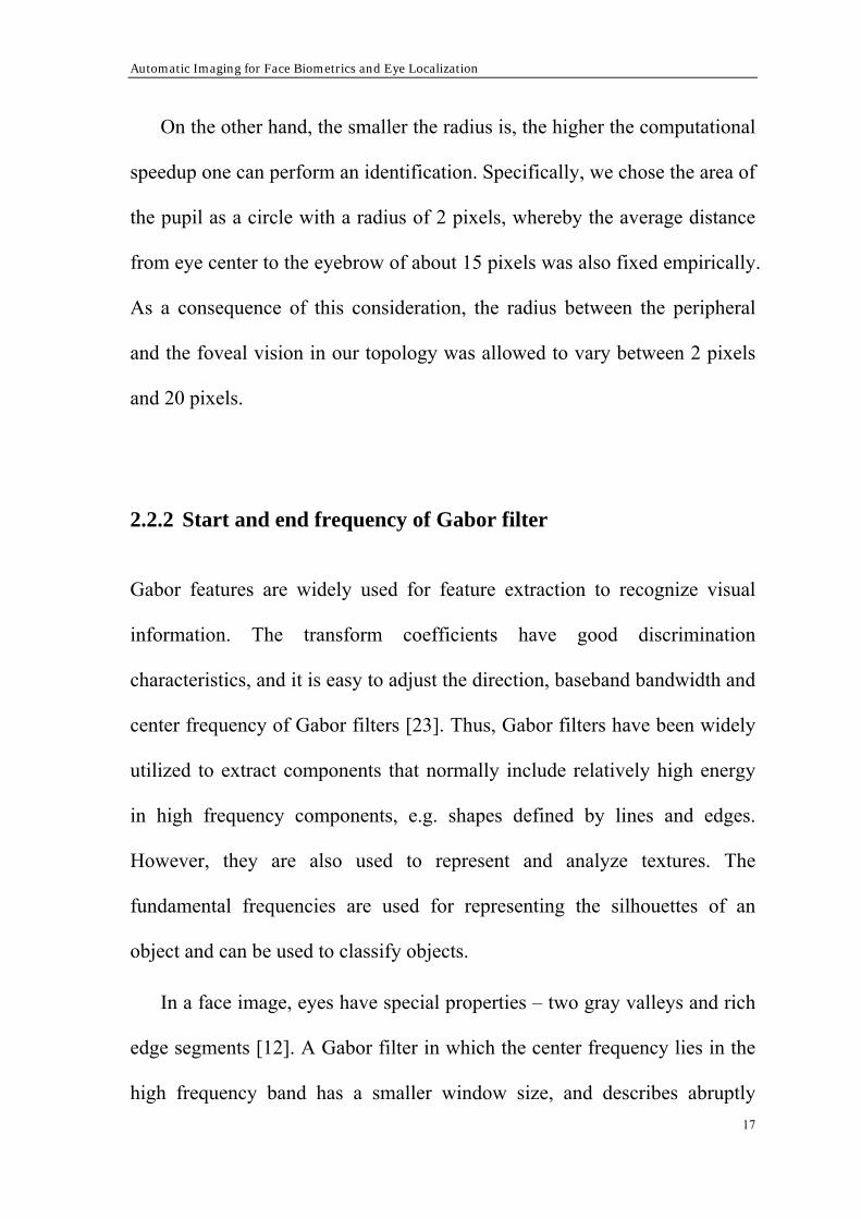
horizontal, and so on. Figure 2-4 illustrates this visually.
Figure 2-3: original face image and target eye-and-brow region
Automatic Imaging for Face Biometrics and Eye Localization
21
2.3.1.1 Single Gabor Filter per retina grid point
In order to enhance computational efficiency and robustness, we represent
features by using Gabor filters which are also non-orthogonal. The Gabor
filters transformation corresponds to multi-scale oriented feature
representation, and at multiple scales, Gabor filters can be used for detecting
oriented features.
In the eye-and-brow region, orientation is the salient characteristic,
which means the signal contains more possibilities in the horizontal
orientation than the vertical orientation. Gabor filters can capture salient
visual properties, such as spatial localization, orientation selectivity.
From the figure 2-4, we can see the first orientation is sensitive to
vertical and the fourth orientation is sensitive to horizontal directions. It
Figure 2-4: Gabor filters on the frequency plane with 5 frequencies and 6 orientations

22
means that the fourth orientation is a good one to identify eye-and-brow
region if we had to choose only one filter. The experimental results are
shown in figure 2-5.
Frequency=4, orientation=4 || Frequency=4, orientation=6 || Frequency=2, orientation=4
Figure 2-5: Scalar product results by sample Gabor filters
2.3.1.2 Specific filter for each retinal point
For a face, though eye and eyebrow look like they are horizontal, the
features of other regions are obviously non-horizontal. Accordingly
appropriate filters need to be compiled with the corresponding frequency
and orientation in mind. That means that if we only used a single filter and
having the same frequency and orientation to obtain the scalar products with
local images around every grid point, our features will not be as descriptive
as these would be, compared to choosing the single filter in accordance with
the dominant orientation and frequency occurring around each grid point.
On the other hand, using all filters (5 frequencies and 6 orientations
based on a certain start and end frequency), with 68+1 retina sampling grid

Automatic Imaging for Face Biometrics and Eye Localization
23
points for each artificial retina, we get a 2070 dimensional feature vector
(30X69).
We picked up the filter producing the highest response among the 30
dimensions at every grid point. Accordingly, we then get a 1*69 vector, for
the artificial retina. The filter chosen for every grid point corresponds to a
frequency and orientation that yields the highest share of the representation
compared to using all filters. Table 2-2 shows the automatically chosen
filters and the directions they represent. Choosing different filters for
different grid points is made for the average of the artificial eye feature
vector having 2070 dimensions.
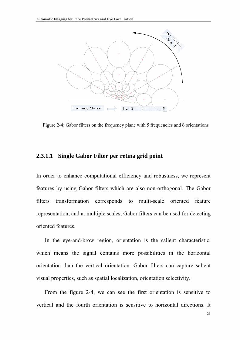
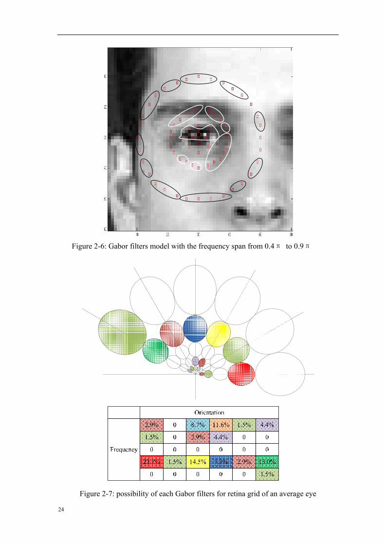
Figure 2-6 shows the specific frequency and orientation filter chosen for
each different retina point. We circle out the regions with the same
orientation. In order to verify the capability of the Gabor filters to select the
eye-and-brow regions, experiments are conducted. The used filter bank is
illustrated by figure 2-7.
Table 2-2: Relationship between the order of the combination and the corresponding frequency
and orientation
Orientation
○1 (1,1) ○2 (1,2) ○3 (1,3) ○4 (1,4) ○5 (1,5) ○6 (1,6)
○7 (2,1) ○8 (2,2) ○9 (2,3) ○10 (2,4) ○11 (2,5) ○12 (2,6)
○13 (3,1) ○14 (3,2) ○15 (3,3) ○16 (3,4) ○17 (3,5) ○18 (3,6)
○19 (4,1) ○20 (4,2) ○21 (4,3) ○22 (4,4) ○23 (4,5) ○24 (4,6)
Frequency
○25 (5,1) ○26 (5,2) ○27 (5,3) ○28 (5,4) ○29 (5,5) ○30 (5,6)
24
Figure 2-6: Gabor filters model with the frequency span from 0.4π to 0.9π
Figure 2-7: possibility of each Gabor filters for retina grid of an average eye

Automatic Imaging for Face Biometrics and Eye Localization
25
Figure 2-8 shows, the distribution of Gabor filters located on a retina
grid under frequency from 0.1π to 0.5π using the training set discussed in
section 2.2.2. We can see that some details are ignored by the low frequency
filter.
Figure 2-8: Gabor filters model with the frequency span from 0.1π to 0.5π
2.3.2 Computing the average eye
Using the parameters we have selected, we perform scalar products between
each retina point of one eye and the corresponding frequency and orientation,
and then we obtain a matrix of 69 feature points for one eye. Looping this
procedure for every person in the training set, we obtain a feature matrix,
and then we calculate the mean value of this matrix such that we obtain a 69

26
dimensional vector. The average vector contains 69 average features of one
eye, and we call this vector the ‘average eye’. The training procedure is
shown as follow:
For i = 1 : (num of different eye pictures in the training set)
1). Select visual eye centre O manually.
2). Place 69 retina points (P1…P69) around this eye centre O.
3). Compute scalar product between each retina point and
corresponding Gabor filter Gi, to obtain the feature vector FV.
4). Normalize feature vector FV.
End
5). Compute the average features for all training people.
At step (1), for a new image, we first select the eye centre manually, then
perform step (2), we set a retina model with the centre of this eye centre,
every retina grid point Pi is retained for the feature extraction. At step (3),
the Gabor feature vector is computed using the scalar product. This vector
describes the neighborhood of each retina point Pi. A single Gabor filter Gi
is a 2-D complex valued filter [5], which has a certain frequency and
orientation as we have selected in section 2.2.1.2.
2.3.3 Weights
The variance of a probability distribution is a measure of statistical

Automatic Imaging for Face Biometrics and Eye Localization
27
dispersion, which is used to capture its scale, or degree of being spread out
[1]. Thus, we compute variance to the normalized feature vector FV, and
then the weights are set as the inverse of the corresponding variance, finally
normalize the weights such that they sum up to 1.
.
2.4 Locate eye center
We first illustrate the whole localization procedure in the testing part, then
import two methods to determine eye center, finally we set threshold for
detection performance.
2.4.1 The strategy of locating eye center
The parameters of the testing part are the same as in the training data. The
strategy of determining eye center consists of comparing the feature vector
of 69 retina points of one pixel in the test picture to the reference feature
vector of the eye center. The comparison is done by obtaining a quadratic
sum of vector element differences. This is done for every pixel of the test
image whereby the said pixel is assumed to be an eye center. The pixel with
Sum of Square Error (SSE) holds the most similarity (best matches) to the
eye center. That point is then marked as an eye (not specific to a person).
The testing procedure is shown as follow:

28
For m = 1: (number of y-coordinate)
For n = 1: (number of x-coordinate)
1). Select the current pixel at n,m as the candidate point for an eye.
Call it O.
2). Place 69 retina points (P1…P69) around this test centre O.
3). Compute the scalar product between each retina point Pi and its
corresponding Gabor filter Gi, for getting feature vector FV.
4). Normalize feature vector FV.
5). Compute the difference of feature vector FV and the average eye
vector.
End
End
6). Pick up the location yielding SSE or Schwartz inequality among
differences computed at step 5 as the eye-location.
2.4.2 Compare testing feature with training feature
Using a similar strategy, we can get the feature vector of the test image at a
candidate position and the average feature vector of the training set at the
artificial retina centre. After this step we can compare this feature vector to
an average vector obtained on the training set using different techniques as
discussed next.
Automatic Imaging for Face Biometrics and Eye Localization
29
2.4.2.1 The Sum of Square Error (SSE)
The quadratic sum of the difference of features between the model and the
test image gives a global matching score, and the pixel with the least
difference holds the most similarity to a typical eye, which means a facial
landmark has been found.
Note that, Sum of Square Error (SSE) is actually a value between 0 and 1.
“0” means the two vectors have the highest similarity, and “1” means the
lowest similarity. This is because the difference is normalized by the sum of
the norms of the two vectors.
2.4.2.2 Schwartz inequality
Schwartz inequality states that, given two vectors f and g, in a vector space
V and a scalar product <, > over V, |<f, g>|<=||f|| · ||g||.
Note that, Schwartz inequality is actually a value between 0 and 1. “1”
means the two vectors have the highest similarity, and “0” means the lowest
similarity.
2.4.3 Detection performance
Detection performance was evaluated by Euclidean distance and visual
inspection. We compared the detected eye positions with the foveal positions

30
which we manually selected before; the performance is described by the
success rate of eye localization [15].
We set three thresholds on distance to the ideal eye centers (marked
manually), which are less than, or equal to, 5 pixels, 3 pixels and 1 pixel. We
circle out the threshold region in figure 2-9, figure 2-9(a) is in the
handed-over image and figure 2-9(b) is in the original picture.

Automatic Imaging for Face Biometrics and Eye Localization
31
Figure 2-9(a) the threshold region in the handed-over image
Figure 2-9(b) the threshold regions in the original image

32

Automatic Imaging for Face Biometrics and Eye Localization
33
Chapter 3
Client identification
3.1 Identification model
Client authentication is a research field related to face recognition. Since the
human face can always undergo variations in appearance and changes in
facial expressions, poses, scales, shifts, and lighting conditions constantly
occur, face recognition has long been facing many challenges. Our proposed
system verifies the claimed identity of the subject, with tolerance to facial
expression variations. The flowchart of our identification approach is
presented in figure3-1.
The first goal in our proposed system is to construct a client database
that includes those clients we intend for future recognition. In our system,
we selected 5 groups of subjects from the XM2VTS database as inputs. In
the previous chapter, we explain that facial landmark location in our case is
an eye location. We then give the system a prepared frame where a face is
already delineated by a face detection technique. With the help of eye
localization techniques discussed previously, the system jumps to the
assumed position, either to the center of the right or the left eye. Then the
retinotopic sampling grid is placed on the eye area, with its first grid point

34
Image database/client
group
Image standardization
Data preparing
Facial Landmarks
location
Sampling grid placing
Feature extraction
Client database
Image database/camera
frame
Image standardization
Data preparing
Facial Landmarks
location
Sampling grid placing
Feature extraction
Matching
Client identified /Access denied
right on the eye center. Preferably, the sampling grid will cover the fovea of
the eye area. As indicated, we would mainly extract the biometric feature of
the eye fovea. This means that we assume different people have different
biometric features around their eyes.
Figure3-1: Flow chart of the identification system
Automatic Imaging for Face Biometrics and Eye Localization
35
This is the basic concept of our biometric identification. One could
easily figure out the advantage of using a retinotopic sampling grid
remembering that feature extraction is usually very time-consuming. Closer
to the eye center, more feature are retained; this means that, by
implementing retinotopic sampling grid, we maximize the discriminative
information we want to keep and reduce the computational costs. After
positioning the retinotopic sampling grid, we associate with each grid point
orientation and frequency sensitive cells, each having a receptive field of its
own, (see figure3-2) represented by the spatial extensions of the Gabor
filters. Here we constructed 6-absolute frequency channels, and 6-orientation
channels using a Gabor filter bank of 36 filters. A receptive field can be
viewed as a simple model of theV1 cell in the primary visual cortex.
Accordingly, in our experiments, we calculated 36 different Gabor filter
responses at each point of the artificial retina, with the help of equation 9. It
is worth noting that the Gabor filter magnitude response is invariant to
sinusoids, reaching a maximal response when 0ξ is the actual frequency
(and 0η the orientation) of the filter. When analysis of local image structures
with small details are needed, higher frequency filters will show a higher
filter response k. In contrast, applying lower rather than higher frequencies
shall give greater magnitudes k, when a coarser and larger structure of a face
is focused on by the feature extraction. Because of the complexity of the
area eye we cover, both finer small structure and coarser larger structure can

36
be analyzed simultaneously, and we also hope that more discriminative
information for face recognition will be available.
Figure3-2: Receptive fields of Gabor filters
For each grid point of one eye, we calculate the scalar product between
one out of 36 filters, with its corresponding local neighborhood. This results
in a feature vector of length 2484, for representing the identity of each
subject. At this step, we store every feature representing each client identity
on the hard disk for future verification of that client, when she/he wants to
be authenticated.
When a new camera frame is given, we follow the same routine as the
previous step that we followed to obtain the training reference model of
clients. Then we need to have a similarity measurement technique for
matching the current image features with the reference features already in
the client feature database we constructed. This technique is explained in the
next section. The details of experiments are given in Chapter 4.

Automatic Imaging for Face Biometrics and Eye Localization
37
3.2 The matching concept
In our proposed system for matching two Gabor feature vectors representing
identities, we studied two similarity measurement methods, Schwartz
inequality and the method of sum of squared error.
3.2.1 Schwartz inequality
Schwartz inequality, already discussed previously in the context of eye
localization, states that given two vectors, f and g, in a vector space V, and a
scalar product <, > over V, then we have the inequality |<f, g>|<=||f|| · ||g||. It
can also be used in the context of identity verification. Also, Schwartz
inequality can be interpreted as measuring the angle between two feature
vectors each representing an identity:
,cos|| |||| ||
xyx y
x yθ < >
= (9),
Here, X and Y are two vectors in a vector space V, and the equation
results a in a value between [-1, 1].
After extracting the biometric feature of the eye area of a subject, we
calculate both the norm of the feature vector and the reference vector
previously stored, and applying equation (9) to receive a similarity score
between the two vectors. Note that we use the absolute value of the scalar

38
product between the two feature vectors; our similarity measure is actually a
value between 0 and 1 because all of our vector elements are magnitudes,
meaning that they are never negative. The final score “1” means the two
vectors have the highest similarity, and “0” means the lowest similarity.
3.2.2 SSE
The method of sum of squared error is often applied in statistical contexts,
particularly regression analysis. It can be interpreted as a method of fitting
data. The sum of squared residuals has its least value when the two vectors
are very similar, a residual being the difference between an observed value
and the value predicted by the model (equation 10). This residual sum
described by Carl Friedrich Gauss around 1794 who attempted to minimize
the SSE by changing the model parameters.
2
1( )
n
i ii
X Y=
−∑ (10)
Here, X and Y are two vectors in a vector space V. In our system, at
matching phase, we derived two Gabor feature vectors, each representing
client or potential client. Applying (10) on two normalized biometric
features, we then derive our similarity measure between the model (of the
client stored previously) and the measurements made on the current picture
of the client. Detailed information on the experiment result is discussed in
chapter 4.

Automatic Imaging for Face Biometrics and Eye Localization
39
3.3 Training by weights
In chapter 3.1, we discussed placing a retinotopic sampling grid on the fovea
of an eye in order to collect feature information of that area. In all of 69
positions on an eye area, which position is more important than the others
and which one is the weakest position, is the subject of the discussion in this
paragraph. After establishing the important position, one could give a higher
weight value for that position to declare its importance for identifying the
clients. The other points are, accordingly, treated as weaker and will
contribute less to identification. Such points would be given a small weight
value. The key factor of determining which grid points are strong verifiers in
the process of identification is the stability of the performance of those very
points when they are extracted for a number of clients. A point that always
performs consistently is considered an important grid position; in this case
we introduce variance as an indication for measuring the importance of those
grid positions. In probability theory, the variance of a random variable,
probability distribution, or sample is a measure of statistical dispersion,
averaging the squared distance of its possible values from the expected value
(mean). The mean is a way to describe the location of a distribution, and the
variance is a way to capture its scale or degree of consistency or being
spread out. In general, the population variance of a finite population of size
N is given by

40
2 2
1
1 ( )N
ii
X XN
σ=
= −∑ (11)
where X is the population mean.
In our system, we construct two groups of images for the training weight
for each position. In one training group, we have 40 different images of
different people, while in the other training group we also have 40 images of
the same group of subjects, but with different facial expression or hair
changes. For one same person, we extract the Gabor responses of the same
point out of 69 positions on a sampling grid in two training groups, calculate
the similarity of the two response vectors and give it a score. Then we do the
same for the artificial retina point but for a different person. After this we get
a group of 40 scores for one particular retina point. The variance of this
position 21σ , which represents the stability of this position, is derived.
Variances for other positions are also obtained in this way. Higher variance
means lower stability. In this case, our system uses the reciprocal of variance
2
1σ
for calculating the weight of a particular grid point. Figure 3-3 shows
training one weight for one particular point of 69 retinotopic sampling grid
points.

Automatic Imaging for Face Biometrics and Eye Localization
41
Figure 3-3: An example of the training process for variance of one grid point
+ + + …………
Score1 Score2 ……. Score40 21σ

42

Automatic Imaging for Face Biometrics and Eye Localization
43
Chapter 4 Experiments and results
In this chapter, the experimental results of all proposed methods and
algorithms are presented, and a detailed analysis of those results is also
included. Detailed information on the laboratory environment is described in
section 1.3.
4.1 Landmark localization tests
4.1.1 Parameters instruction
Facial landmark detection tests were run on a total of 110 images from the
XM2VTS. For each handed-over image, there is only one eye included, due
to locating two eyes’ centers separately; the following experiments use right
eyes as samples.
The training set is consisted of 50 persons, they are all non-glasses,
frontal face, no expression, and size of the handed-over images (by the face
localization system) are 60×60 pixels.
The testing sets are separated into three groups. The first one is the same
as the training set, which has the same 50 people, and the second one and
third one both consisted of 30 different people; the total number of people in
the three groups is 110.

44
Succeed Rate
Time calculation is under the configuration of the PC, which is Intel
Core 2, 2.1 GHz, 800MHz FSB, 3MB L2 cache, 2GB DDR2.
4.1.2 Experimental results
We mainly adopt four combinatorial methods for testing. The first two
methods are the Sum of Square Error (SSE), with and without weights, and
the other two methods are Schwartz inequality, with and without weights.
Visually, eyeball region, including the white of the eye, is less than or
equal to 5 pixels with the centre of fovea: this is what we called an
acceptable result. Pupil region is less than or equal to 3 pixels: this is what
we called the perfect result. The region which is less than or equal to 1 pixel
is only for reference, in order to evaluate the accuracy.
Experimental results are shown from table 4-1 to table 4-4. Each table
describes the success rate achieved in the thresholds of less than or equal to
5 pixels, 3 pixels and 1 pixel, by the groups of 50 people, which is the same
as the training set, another two groups, each of 30 people.
Table 4-1: Sum of Square Error (SSE) without weights
Threshold
Group ≤5 pixels ≤3 pixels ≤1 pixels
Seconds required for the operation
50p training set 100% 94% 50% 13.845
30p1 93% 90% 73% 13.545
30p2 100% 100% 70% 13.790
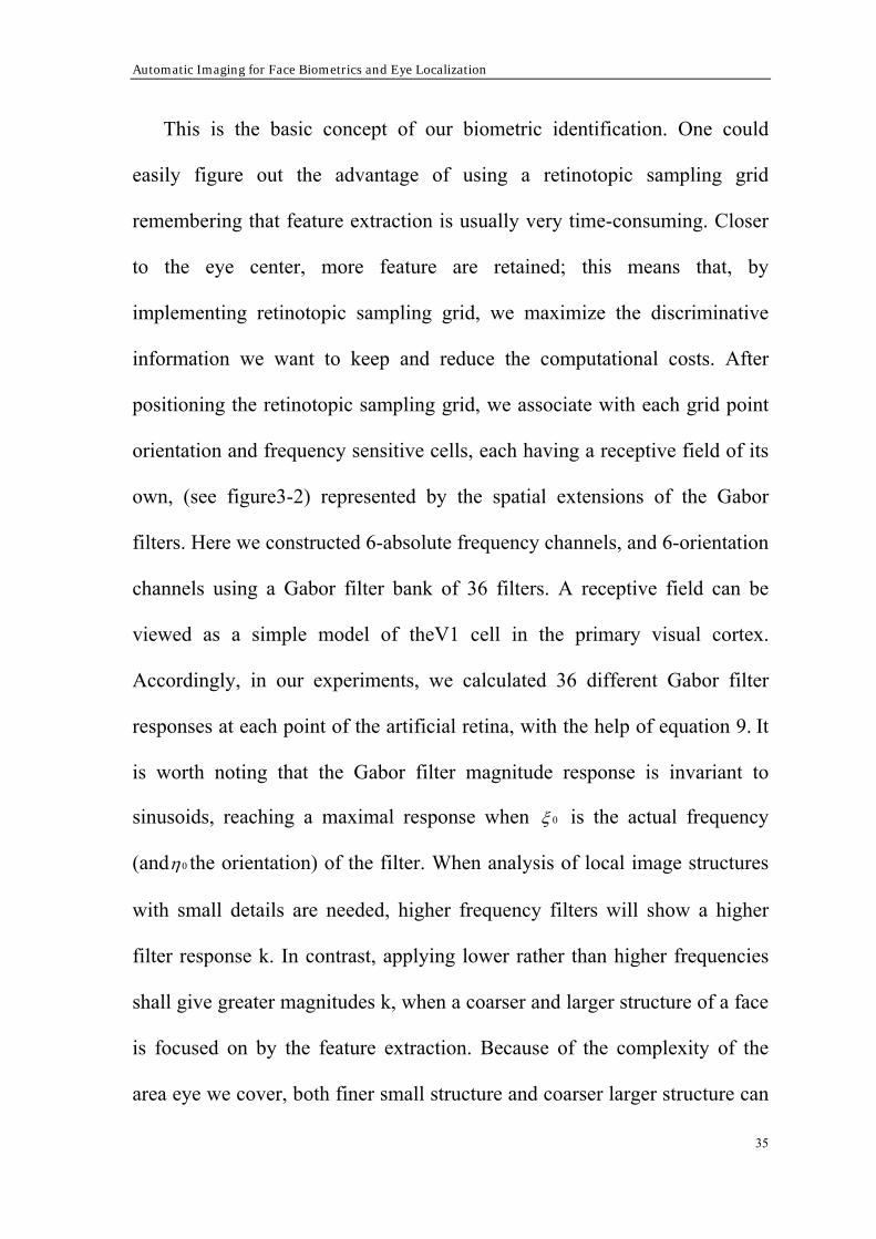
Average Success Rate 98% 95% 64% 13.727
Automatic Imaging for Face Biometrics and Eye Localization
45
Succeed Rate
In this table, success rate of the acceptable region is 98%, which means 2
images out of 110 images are not detected. Success rate of the perfect region
is 95%, which means 6 images out of 110 images are not detected, whereas
success rate of the reference region is still 64.43%, which means the
detected eye center of 97 images are exactly same as the visual fovea.
The average time for detecting one eye is 13.727 seconds, using
MATLAB 7.0, running in our PC.
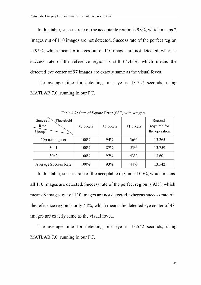
Table 4-2: Sum of Square Error (SSE) with weights
Threshold
Group ≤5 pixels ≤3 pixels ≤1 pixels
Seconds required for the operation
50p training set 100% 94% 36% 13.265
30p1 100% 87% 53% 13.759
30p2 100% 97% 43% 13.601
Average Success Rate 100% 93% 44% 13.542
In this table, success rate of the acceptable region is 100%, which means
all 110 images are detected. Success rate of the perfect region is 93%, which
means 8 images out of 110 images are not detected, whereas success rate of
the reference region is only 44%, which means the detected eye center of 48
images are exactly same as the visual fovea.
The average time for detecting one eye is 13.542 seconds, using
MATLAB 7.0, running in our PC.

46
Succeed Rate
Succeed Rate
Table 4-3: Schwartz inequality without weights
Threshold
Group ≤5 pixels ≤3 pixels ≤1 pixels
Seconds required for the operation
50p training set 100% 94% 50% 13.441
30p1 93% 90% 73% 14.112
30p2 100% 100% 70% 13.941
Average Success Rate 98% 95% 64% 13.831
In this table, success rate of the acceptable region is 98%, which means 2
images out of 110 images are not detected. Success rate of the perfect region
is 95%, which means 6 images out of 110 images are not detected, whereas
success rate of the reference region is still 64%, which means the detected
eye center of 97 images are exactly same as the visual fovea.
The average time for detecting one eye is 13.831 seconds, using
MATLAB 7.0, running in our PC.
Table 4-4: Schwartz inequality with weights
Threshold
Group ≤5 pixels ≤3 pixels ≤1 pixels
Seconds required for the operation
50p training set 100% 90% 42% 13.729
30p1 93% 77% 50% 13.828
30p2 93% 67% 30% 13.545
Average Success Rate 95% 78% 41% 13.701
In this table, success rate of the acceptable region is 95%, which means 4
images out of 110 images are not detected. Success rate of the perfect region
is 78%, which means 24 images out of 110 images are not detected, whereas

Automatic Imaging for Face Biometrics and Eye Localization
47
success rate of the reference region is only 41%, which means the detected
eye center of 45 images are exactly same as the visual fovea.
The average time for detecting one eye is 13.701 seconds, using
MATLAB 7.0, running in our PC.
From the tables above, we can find some regular patterns as follow:
1. In the Sum of Square Error (SSE) method, using weights could get the
best results, 100% success rate, in less than or equal to 5 pixels, but
could get worse results in less than or equal to 3 pixels.
2. In the Schwartz inequality method, not using weights could get better
results than using weights.
3. For non-weights, the results are exactly same under both Sum of Square
Error (SSE) method and the Schwartz inequality method.
4. On the whole, without using weights, the result in the perfect area could
be 95% in both methods; while, with using weights, the result in the
perfect area is only 86% in both methods.
5. The time required for detecting one eye center is about 13.5 seconds,
which is also depending on the PC configuration.
Experimental results all show reliable eye detection performance. Figure
4-1 shows some identified results in the handed-over image and the original
image.

48
Figure 4-1(a): Successful identified results in the perfect region
Figure 4-1(b): Successful identified results in the acceptable region
Figure 4-1(c): Failing identified results

Automatic Imaging for Face Biometrics and Eye Localization
49
4.2 Client identification tests
In this section, in accordance with the theories and methods proposed in
chapter 3, the implementation of our system for identification and its test
results are presented.
4.2.1 Determining model parameters
A training-set of 10 images is formed, of which 5 pictures are captured by
web-camera and another 5 pictures are from the XM2VTS database. In this
training set, there are 3 women and none of the subjects wear glasses. In the
testing set, we have 13 client images, of which 3 are impostors without
glasses. In the identification process, all 10 clients are correctly identified
and 3 impostors are rejected. We use the above small training set and testing
set to determine the radius of our retina, number of frequency channels,
number of orientation channels and suitable frequency range based on the
theories and algorithm described in Chapter3.
Firstly, identification based on alternative retina radius range is tested, as
mentioned in chapter 3. We empirically choose the radius range of retina
from 10.7 to 50 or 60 pixels, according to the size of eye area in a camera
frame. Basically, this range covers the eye area and excludes information of
other biometric features such as ears, forehead or hair. A 5-frequency
channels 6-orientation channels Gabor filter bank is constructed first, with a

50
Similarity
frequency range from 0.1π to 0.5π , and similarity measure is calculated
using Schwartz inequality. Table 4-5 shows the comparison between the two
ranges. We could see that, with radius from 10.7 to 50 pixels, the mean
similarity value of clients has risen compared to the retina radius, from 10.7
to 60, and the mean similarity value of impostors has decreased, which
means the retina radius range from 10.7 to 50 has a better performance in
enlarging the gap between similarity measure of clients and impostors.
Table 4-5: Similarity measure based on alternative retina radius range Group
Radius Range Clients Impostors
10.7-60 0.93 0.90
10.7-50 0.94(↑ ) 0.89 (↓ )
Secondly, we test the effect of the frequency channels employed in our
system on the similarity measure. We compare only using higher frequency
channels with using all channels (the result is shown in table 4-6.) We notice
that a rise in the similarity measure of clients is a good thing, but too much
rise in similarity measure of impostors also ruins the whole performance.
Table 4-6: Similarity measure based on alternative frequency Group
Frequency Clients Impostors
[1 2 3 4 5] 0.93 0.90
[3 4 5] 0.94 (↑ ) 0.94 (↑ )
Similarity

Automatic Imaging for Face Biometrics and Eye Localization
51
Similarity
Next, we compare the Gabor filter bank of 5 frequency channels and 6
frequency channels with the same 6 orientation channels. Table 4-7 shows
there is no change in the mean similarity of clients, and a well achieved
decrease in the mean similarity of impostors, which means a 6 by 6 Gabor
filter bank has a better performance in distinguishing impostors from clients.
Table 4-7: Similarity measure based on alternative Gabor filter bank Group
Filter Bank Clients Impostors
5 by 6 Gabor filter bank 0.93 0.90
6 by 6 Gabor filter bank 0.93 0.87(↓ )
The frequency range of Gabor filter bank is proved to be an important factor
in deciding similarity value. The original start frequency of our filter bank is
0.1π and the end frequency is 0.5π . After we enlarge the range from 0.05π
to 0.7π , the system gains much better performance. Table 4-8 shows the
results.
Table 4-8: Similarity measure based on alternative filter bank frequency range Group
filter bank frequency range
Clients Impostors
0.1π -0.5π 0.93 0.90
0.05π -0.7π 0.96(↑ ) 0.87 (↓ )
Similarity

52
Finally, we take another biometric feature into consideration for our system,
which is the nose feature. The configuration is that the radius range of the
retina is from 10.7 to 50 pixels. A 5-frequency channel 6-orientation channel
Gabor filter bank is constructed with a frequency range from 0.1π to 0.5π ,
and the similarity measure is calculated using Schwartz inequality. Since we
have two different biometric features in our system, we decide to assign
weight for different features. Each eye is given a weight of 40%, and the
nose 20% weight. With the nose feature introduced into our system, we
would improve the performance but in a very limited way. The result is
shown in table 4-9.
Table 4-9: Similarity measure based on different feature information Group
Feature Information Clients Impostors
Without nose 0.93 0.90
With nose 0.94(↑ ) 0.89 (↓ )
4.2.2 Identification tests
In the first identification test, a group of 50 people is chosen from the
XM2VTS database as the training set for reference, and in which 10 people
have glasses. We have another image recording of the same group of 50
people as our testing set, and we add 20 more impostors, of which 4 among
the 20 wear glasses.
Similarity

Automatic Imaging for Face Biometrics and Eye Localization
53
From the experiment results we have gained in last section, we decided
to use a 6 by 6 Gabor filter bank, with frequency range from 0.05π to 0.7π ,
and employ a retina, with radius range from 10.7 to 50 pixels, in our
identification test. The identification rate is the indication of how
successfully we can recognize a person with our system, and this ratio can
be obtained as follows:
Identification Rate = __
client identifiedclient number
We use Schwartz inequality as our similarity measure in the first test,
and the result is 33/40=82.50% clients are correctly identified among those
40 clients without glasses, and only 10% clients with glasses are correctly
identified. Figure 4-2 illustrates a histogram of similarity measurement of
test 1, and we use a threshold of value 0.91. In all, 20 impostors are rejected
by our system.
In the second test, we only have the same 40 people without glasses as
our training set, and choose the corresponding 40 images from the testing set
of test 1 as the testing set with an additional 20 impostors. In this test we
employ SSE as our similarity measure, a histogram of similarity
measurement is shown in figure 4-3.With a false rejection rate of 12.5%, and
false acceptance rate of 10%, we use 0.20 as our threshold, and this results in
an identification rate of 87.5%.
54
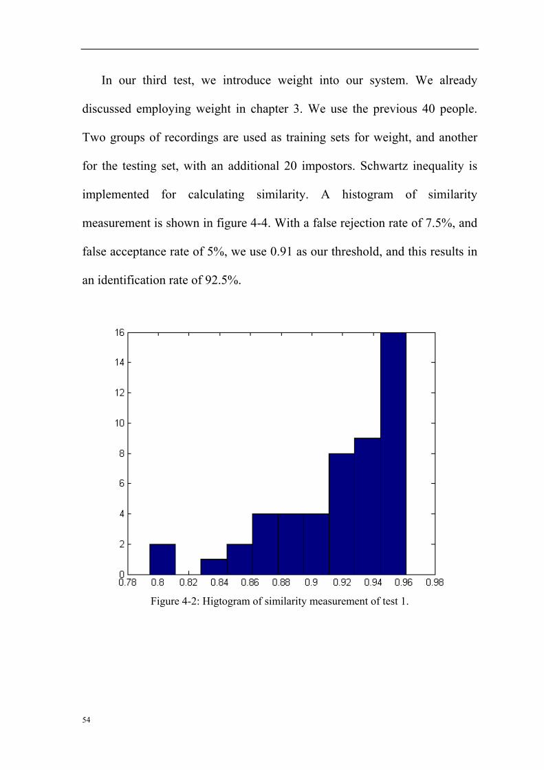
In our third test, we introduce weight into our system. We already
discussed employing weight in chapter 3. We use the previous 40 people.
Two groups of recordings are used as training sets for weight, and another
for the testing set, with an additional 20 impostors. Schwartz inequality is
implemented for calculating similarity. A histogram of similarity
measurement is shown in figure 4-4. With a false rejection rate of 7.5%, and
false acceptance rate of 5%, we use 0.91 as our threshold, and this results in
an identification rate of 92.5%.
Figure 4-2: Higtogram of similarity measurement of test 1.

Automatic Imaging for Face Biometrics and Eye Localization
55
Figure 4-3: Higtogram of similarity measurement of test 2.
Figure 4-4: Histogram of similarity measurement of test 3

56
Figure 4-5: Histogram of similarity measurement of test 4
In our last test, we implement weight and use SSE as the similarity
measure in our system. Again, we use the same 40 people as before. Two
groups of recordings are used as training sets for weight and another for the
testing set, with an additional 20 impostors. A histogram of similarity
measurement is shown in figure 4-5. With a false rejection rate of 7.5% and
false acceptance rate of 10%, we use 0.0027 as our threshold, and this results
in an identification rate of 92.5%.

Automatic Imaging for Face Biometrics and Eye Localization
57
Chapter 5 Discussion and conclusion
In our proposed system, the test results of the eye localization are
encouraging with the help of Gabor filter banks, which is a pre-requirement
of the person authentication system. Due to the harsh thresholds we set, we
only use the acceptable area to compare with several similar systems, which
are presented in table 5-1. From the table, the system we proposed is much
better than others. For Ref [12], it uses Gabor-eye model and radial
symmetry operator to locate pupil area; for Ref [17], Gabor filter is under
probabilistic framework to locate eye center; for Ref [19], navigational
routines is proposed. Table 5-1: Comparison of the results with other methods
Groups Yang & Du
[12]
Ma & Ding
[17]
Huang &
Wechsler [19] Ours
Success Rate 95% 94.44% 98.7% 98%
Regarding the differences between the human eye fovea, the average eye
model works at a satisfying level, but an eye location technique for both the
human eyes needs to be developed comparing with the current locating
one-by-one mechanism. The eye localization performance with respect to
time demand can be improved by using dedicated hardware.
58
On client identification, good results have been achieved with Gabor
filter banks and the usage of carefully chosen sampling points and frequency
channels employed in the identification part, which enable its real-time
performance, and need to be improved with a bigger training-set. It is not
realistic to compare the performance of different systems in a quantitative
way, because of the different environments that are implemented. In general,
the algorithm of [2] took about 8 minutes to perform facial landmark
detection and face verification. In our proposed system, it takes no more
than 4 seconds for client identification, and no more than 40 seconds to
perform facial landmark detection and face identification. An EER of 6.0%
has been achieved in the identification process and can be further improved
by training SVM experts [2]. In order to gain a better identification
performance, we could also continue research on introducing other facial
biometrics, such as nose or mouth, into our system. Further research on the
sensitivity with respect to clients with glasses has to be carried out. For
real-time purposes, the possible future work involves implementation of the
whole system, with a faster language such as ’C#’.
Automatic Imaging for Face Biometrics and Eye Localization
59
References
[1] Wikipedia.org
Biometrics
The Free Encyclopedia URL:http://en.wikipedia.org/wiki/Biometric
Viewed: May 15, 2009
[2] F. Smeraldi, J. Bigun
Retinal vision applied to facial features detection and face authentication
Pattern Recognition Letters 23, pp. 463–475, 2002
[3] F. Smeraldi, O. Camona, J. Bigun
Real–Time Head Tracking by Saccadic Exploration
Proceedings of the 5th International Workshop on IEEE Cat. Num. 98TH8354, pp.
684–687, 1998
[4] Josef Bigun Vision with direction: A systematic introduction to image processing and computer vision. Springer, 2006.
[5] J. Bigun, H. Fronthaler, and K. Kollreider
Assuring liveness in biometric identity authentication by real-time face tracking
IEEE International Conference on Computational Intelligence for Homeland Security
and Personal Safety Venice, Italy, 21-22 July 2004
[6] B. Duc, S. Fischer, and J. Bigun.
Face authentication with Gabor information on deformable graphs
IEEE Trans. on Image Processing, 8(4):504–516, 1999.
[7] Ian R Fasel, M. S Bartlett, and J. R. Movellan.
A comparison of Gabor methods for automatic detection of facial landmarks
International conference on Automatic Face and Gesture Recognition, pages
242–248, May 2002.
[8] Al-Amin Bhuiyan, and Chang Hong Liu
On Face Recognition using Gabor Filters
Proceedings of World Academy of Science, Engineering and Technology volume 22
July 2007.

60
[9] David A. Clausi, M. Ed Jernigan
Designing Gabor filters for optimal texture separability
Pattern Recognition 33 (2000) 1835-1849
[10] Josef Bigun
Circular Symmetry Models in Image Processing
Linkoping studies in Science and Technology, Thesis No. 85,
LIU-TEK-LIC-1986:25, Linkoping University, Sweden, September 1986
[11] J. Bigun
Pattern recognition in images by symmetries and coordinate transformation
Computer Vision and Image Understanding, vol. 68, nr. 3, pp. 290–307, 1997
[12] Peng Yang, Bo Du, Shiguang Shan. Wen Gao
A novel pupil localization method based on gaboreye model and radial symmetry
operator
2004 International Conference on Image Processing (IClP), 0-7803-8554-3/04
[13] Hyunwoo Kim, Jong Ha Lee, Seok Cheol Kee
A Fast Eye Localization Method for Face Recognition
Proceedings of the 2004 IEEE International Workshop on Robot and Human
Interactive Communication Kurashiki, Okayama Japan September 20-22, 2004
[14] Geng Du, Fei Su, Anni Cai
Eye Location under Various Illumination Conditions
Proceedings of the International Multi-Conference on Computing in the Global
Information Technology (ICCGI'06), 0-7695-2629-2/06
[15] Peng Wang, Matthew B. Green, Qiang Ji
Automatic Eye Detection and Its Validation
Proceedings of the 2005 IEEE Computer Society Conference on Computer Vision
and Pattern Recognition (CVPR’05), 1063-6919/05
[16] Guo-Sheng Yang, Ting Wang, Huan-Long Zhang
Eye location method based on Gabor wavelet and topographic feature extraction.
Proceedings of the Seventh International Conference on Machine Learning and
Cybernetics, Kunming, 12-15 July 2008. 978-1-4244-2096-4/08

Automatic Imaging for Face Biometrics and Eye Localization
61
[17] Yong Ma, Xiaoqing Ding, Zhenger Wang, Ning Wang
Robust precise eye location under probabilistic framework
Proceedings of the Sixth IEEE International Conference on Automatic Face and
Gesture Recognition (FGR’04), 0-7695-2122-3/04
[18] Shang-Hung Lin, Sun-Yuan Kung, Long-Ji Lin
Face Recognition/Detection by Probabilistic Decision-Based Neural Network.
IEEE Transactions on Neural Networks, vol. 8, No.1, January 1997.
[19] Jeffrey Huang and Harry Wechsler
Visual Routines for Eye Location Using Learning and Evolution
IEEE Transactions on Evolutionary Computation, vol. 4, No.1, April 2000.
[20] Geng Du
Eye location method based on symmetry analysis and high-order fractal feature
IEEE Proceeding Vision Image Signal Process, Vol. 153, No. 1, February 2006.
[21] Yanfang Zhang, Nongliang Sun, Yang Gao, Maoyong Cao
A new eye location method based on Ring Gabor Filter
Proceedings of the IEEE International Conference on Automation and Logistics
Qingdao, China September 2008, 978-1-4244-2503-7/08
[22] Song Li, Danghui Liu, Lansun Shen
Eye Location Using Gabor Transform
Measurement and Control Techniques, 2006, 25(5): 27-29
[23] Richard Buse and Zhi-Qiang Liu
Feature measurement and analysis using Gabor filters
International Conference on Volume 4, Issue , 9-12 May 1995 Page(s):2447 - 2450
vol.4


