
Civil Engineering Infrastructures Journal, 53(1): 15 – 31, June 2020
Print ISSN: 2322-2093; Online ISSN: 2423-6691
DOI: 10.22059/ceij.2019.263233.1503
* Corresponding author E-mail: [email protected]
15
Axisymmetric Scaled Boundary Finite Element Formulation for Wave
Propagation in Unbounded Layered Media
Aslmand, M.1* and Mahmoudzadeh Kani, I.2
1 Ph.D., School of Civil Engineering, College of Engineering, University of Tehran,
Tehran, Iran. 2 Professor, School of Civil Engineering, College of Engineering, University of Tehran,
Tehran, Iran.
Received: 03 Aug. 2018; Revised: 03 Jan. 2019; Accepted: 23 Feb. 2019
ABSTRACT: Wave propagation in unbounded layered media with a new formulation of
Axisymmetric Scaled Boundary Finite Element Method (AXI-SBFEM) is derived. Dividing
the general three-dimensional unbounded domain into a number of independent two-
dimensional ones, the problem could be solved by a significant reduction in required storage
and computational time. The equations of the corresponding Axisymmetric Scaled Boundary
Finite Element (AXI-SBFE) are derived in detail. For an arbitrary excitation frequency, the
dynamic stiffness could be solved by a numerical integration method. The dynamic response
of layered unbounded media has been verified with the literature. Numerical examples
indicate the applicability and high accuracy of the new method.
Keywords: Axisymmetric Scaled Boundary Finite Element Method, Fourier Series, Layered
System.
INTRODUCTION
Correctly modeling of radiation damping in
the infinite soil is one of the major challenges
in wave propagation problem. Finding the
solution of the wave propagation in
heterogeneous layered systems are
unreachable analytically. Almost all of the
existing strategies to model propogation of
waves in layered continuum can be
categorized as the boundary element method
(Karabalis and Mohammadi, 1998; Coulier et
al., 2014, Morshedifard and Eskandari-
Ghadi, 2017), the thin layer method (TLM)
(Lysmer and Waas, 1972; Kausel and
Roesset, 1975) or approximate methods
(Wolf and Preisig, 2003; Baidya et al., 2006;
Nogami and Mahbub, 2005) and semi-
analytical (Gazetas, 1980) or analytical
methods (Ardeshir-Behrestaghi et al., 2013;
Eskandari-Ghadi et al., 2014)
The thin-layer method is semi-analytical
widely used approach in frequency-domain
formed on an axisymmetric Finite Element
formulation. The Finite Element
discretization matches the direction of
layering.
Another semi-analytical approach, the
Scaled Boundary Finite Element Method
(SBFEM) (Wolf, 2003), is particularly
capable of dynamic analysis in unbounded
domains. The SBFEM combines some
important benefits of the Finite Element
method and the boundary element method.

Aslmand, M. and Mahmoudzadeh Kani, I.
16
Not only does it reduce the spatial dimension
of the problem but it also doesn’t require any
fundamental solution. The material
anisotropy can be implemented
straightforwardly by modification of the
constitutive matrix. A combined SBFE-FEM
formulation could be used for dynamic SSI
problems (Genes, 2012; Yaseri et al., 2012;
Syed and Maheshwari, 2015; Rahnema et al.,
2016).
SBFEM is originally uses a scaling center
from which the whole boundary shall be
observable. By the geometry transformation,
it leads to an analytical formulation in the
radial direction which could be solved
numerically in the circumferential direction.
Some modified SBFE formulations for
parallel boundaries two-dimensional domains
(Li et al., 2005), three-dimensional prismatic
domains (Krome et al., 2017) and
axisymmetric domain (Doherty and Deeks,
2003) have been presented. However, none of
these formulations can be utilized to model a
truly three-dimensional layered media. In
order to overcome this shortcoming, the
scaling center is replaced by a scaling line in
the modified formulation of (Birk and
Behnke, 2012). It fully couples the 3D FEM
with 2D SBFEM. In order to reduce the
computational cost and accuracy of the
solution, the formulation of (Birk and
Behnke, 2012) has been modified to an
axisymmetric SBFEM which only a line
discretization is needed to find the solution.
AXI-SBFEM
Consider a scaling line, identical to the axis
of symmetry (the z-axis) in AXI-SBFEM as
shown in Figure 1. The radial direction ξ is
perpendicular to the scaling line. ξ is 0 at the
z-axis and 1 at the line S.
In this paper, the line S is revolved around
the axis of symmetry in order to define the
domain boundary, as shown in Figure1. The
corresponding transformation is formulated
as:
𝑟 = 𝜉. 𝑟𝑠 (𝑠) (1a)
𝑧 = 𝑧𝑠(𝑠) (1b)
𝜃 = 𝜃 (1c)
The displacement components of an
axisymmetric solid in the cylindrical
coordinate system (r, z, 𝜃) can be written as:
Fig. 1. Axisymmetric domain modeled by SBFEM

Civil Engineering Infrastructures Journal, 53(1): 15 – 31, June 2020
17
𝑢𝑟(𝑟, 𝑧, 𝜃) =∑ 𝑢𝑟(𝑟, 𝑧, 𝜃, 𝑛)∞
𝑛=0
= ∑(𝑢𝑟𝑠
∞
𝑛=0
(𝑟, 𝑧, 𝑛)𝑐𝑜𝑠𝑛𝜃
+ 𝑢𝑟𝑎(𝑟, 𝑧, 𝑛) sin 𝑛𝜃)
(2a)
𝑢𝑧(𝑟, 𝑧, 𝜃) =∑ 𝑢𝑧(𝑟, 𝑧, 𝜃, 𝑛)∞
𝑛=0
= ∑(𝑢𝑧𝑠
∞
𝑛=0
(𝑟, 𝑧, 𝑛)𝑐𝑜𝑠𝑛𝜃
+ 𝑢𝑧𝑎(𝑟, 𝑧, 𝑛) sin𝑛𝜃)
(2b)
𝑢𝜃(𝑟, 𝑧, 𝜃) =∑ 𝑢𝜃(𝑟, 𝑧, 𝜃, 𝑛)∞
𝑛=0
= ∑(−𝑢𝜃𝑠
∞
𝑛=0
(𝑟, 𝑧, 𝑛)𝑠𝑖𝑛 𝑛𝜃
+ 𝑢𝜃𝑎(𝑟, 𝑧, 𝑛) cos 𝑛𝜃)
(2c)
The governing equation for the linear
elstodynamics state
�̅�𝑇𝜎 + 𝜔2𝜌𝑢 = 0 (3)
where 𝜎, u and �̅�: are stresses, displacements
and the equilibrium operator in cylindrical
coordinate. The strains follow from the
displacements as
𝜖 = 𝐿𝑢 (4)
which L: is a differential operator in
cylindrical coordinate and can be found in
Aslmand et al. (2018). The approximate
solution of Eq. (3) is obtained using a Fourier
series in the direction of 𝜃 and linear shape
functions along the S which leads to a series
of ODEs in terms of 𝜉. Hence, a solution is
written in the form
{
𝑢𝑟(𝜉, 𝑠, 𝜃)𝑢𝑧(𝜉, 𝑠, 𝜃)𝑢𝜃(𝜉, 𝑠, 𝜃)
}
= ∑{[𝐹𝑢𝑠(𝜃, 𝑛)][𝑁(𝑠)}{𝑢𝑠(𝜉, 𝑛)}
∞
𝑛=0
+ [𝐹𝑢𝑎 (𝜃, 𝑛)][𝑁(𝑠)]{𝑢𝑎 (𝜉, 𝑛)}}
(5)
where
[𝐹𝑢𝑠(𝜃, 𝑛)]
= [cos𝜃 0 00 cos 𝜃 00 0 − sin𝑛𝜃
] , [𝐹𝑢𝑠(𝜃, 𝑛)]
= [sin n𝜃 0 00 sin n 𝜃 00 0 cos 𝑛𝜃
]
(6)
[N(s)]: is the shape functions matrix, and
{𝑢𝑠(𝜉, 𝑛)} and {𝑢𝑎(𝜉, 𝑛)}: stand for the
variation of the nodal displacement in the 𝜉
direction for the symmetric and anti-
symmetric Fourier terms, respectively.
Mapping to the coordinate system of
scaled boundary, the linear operator L is
broken in parts such that:
[𝐿] = [𝐿1]𝜕
𝜕𝑟+ [𝐿2]
𝜕
𝜕𝑧+ [𝐿3]
1
𝑟
+ [𝐿4]1
𝑟
𝜕
𝜕𝜃+ [𝐿5]
1
𝑟 𝜕
𝜕𝜃
(7)
The operators 𝛿/𝛿𝑟 and 𝛿/𝛿𝑧: are mapped
to the scale boundary coordinate and the
operator is then expressed as:
[𝐿] = [𝑏1(𝑠)]𝜕
𝜕𝑟+ [𝑏2(𝑠)]
𝜕
𝜕𝑧
+ [𝑏3(𝑠)]1
𝑟
+ [𝑏4(𝑠)]1
𝑟
𝜕
𝜕𝜃
+ [𝑏5(𝑠)]1
𝑟 𝜕
𝜕𝜃
(8)
where [𝑏1] to [𝑏5] can be found in Aslmand
et al. (2018). Multiplying Eq. (8) by Eq. (5)
and substituting into strain-stress
relationship, terms can be gathered resulting
the following approximate stresses:

Aslmand, M. and Mahmoudzadeh Kani, I.
18
{𝜎(𝜉, 𝑠, 𝜃)} =
{
𝜎𝑟(𝜉, 𝑠, 𝜃)
𝜎𝑧(𝜉, 𝑠, 𝜃)
𝜎𝜃(𝜉, 𝑠, 𝜃)
𝜏𝑟𝑧(𝜉, 𝑠, 𝜃)
𝜏𝑧𝜃(𝜉, 𝑠, 𝜃)
𝜏𝑟𝜃(𝜉, 𝑠, 𝜃)}
= ∑{[𝐷(𝑠)][𝐹𝜀𝑠(𝑛, 𝜃)]([𝐵1
∞
𝑛=0
(𝑠)] {𝑢𝑠(𝜉, 𝑛)], 𝜉 (1
𝜉[𝐵2(𝑠, 𝑛)]
+ [𝐵3(𝑠)]) {𝑢𝑠(𝜉, 𝑛)})
+ [𝐷(𝑠)][ 𝐹𝜀𝑎(𝑛, 𝜃)]([𝐵1(𝑠)], 𝜉 (
1
𝜉[𝐵2(𝑠, 𝑛)] + [𝐵3(𝑠)]) {𝑢𝑎(𝜉, 𝑛)})}
(9)
where the terms
[𝐵1 (𝑠)] = [𝑏1(𝑠)][𝑁(𝑠)] (10)
[𝐵2(𝑠, 𝑛)] = [ [𝑏3(𝑠)] + 𝑛 [𝑏4(𝑠)]
− 𝑛 [𝑏5(𝑠)]] [𝑁 (𝑠)] (11)
[𝐵3(𝑠)] = [𝑏2(𝑠)][𝑁(𝑠)],𝑠 (12)
are introduced for convenience. [ 𝐹𝜀𝑠(𝑛, 𝜃)]
and [ 𝐹𝜀𝑎(𝑛, 𝜃)]: stand for the variation in the
circumferential direction.
[ 𝐹𝜀𝑠(𝑛, 𝜃)] =
[ cos𝑛 𝜃00000
0cos 𝑛𝜃0000
00
cos𝑛𝜃 000
000
cos 𝑛𝜃00
0000
− sin𝑛𝜃0
00000
− sin𝑛𝜃]
(13)
and
[ 𝐹𝜀𝑠(𝑛, 𝜃)] =
[ sin𝑛 𝜃00000
0sin 𝑛𝜃0000
00
sin𝑛𝜃 000
000
sin𝑛𝜃00
0000
cos 𝑛𝜃0
00000
cos 𝑛𝜃]
(14)
The virtual work’s principle for the
dynamic case states:
𝛿𝑈 + 𝛿𝐾 − 𝛿𝑊 = 0 (15)
where U, K and W: are internal strain energy,
structure’s kinetic energy and external work
caused by boundary traction {𝑡(𝑠, 𝜃)}, respectively (It is supposed that all of the
surface tractions are in the near field). The
contribution of the three terms to the virtual
work will be derived in the following. To
derive these three terms, the following form
of virtual displacement.
{𝛿𝑢 (𝜉, 𝑠, 𝜃)}
= ∑{[𝐹𝑢𝑠(𝑛, 𝜃)] [𝑁(𝑠)]{𝛿𝑢𝑠(𝜉, 𝑛)}
∞
𝑛=0
+ [𝐹𝑢𝑎(𝑛, 𝜃)] [𝑁(𝑠)]{𝛿𝑢𝑎(𝜉, 𝑛)}]
(16)

Civil Engineering Infrastructures Journal, 53(1): 15 – 31, June 2020
19
is applied to the structure, where {𝛿𝑢𝑠(𝜉, 𝑛)} and {𝛿𝑢𝑎(𝜉, 𝑛)} includes symmetric and anti-
symmetric virtual nodal displacements for the
nth term of the Fourier series. The
corresponding virtual strain field proceed
from Eq. (9) as:
{𝛿휀(𝜉, 𝑠, 𝜃)} = ∑ {[𝐹𝜀𝑠(𝑚, 𝜃)] ([𝐵1(𝑠)] {𝛿𝑢𝑠(𝜉,𝑚)}, 𝜉(
1
𝜉[𝐵2(𝑠, 𝑚)]
∞
𝑚=0
+ [𝐵3(𝑠)]) {𝛿𝑢𝑠(𝜉,𝑚)}[𝐹𝜀𝑎(𝑚, 𝜃)]([𝐵1(𝑠){𝛿𝑢𝑎(𝜉,𝑚)}, 𝜉 (
1
𝜉[𝐵2(𝑠,𝑚)]
+ [𝐵3(𝑠)]){𝛿𝑢𝑎(𝜉,𝑚)})}
(17)
The virtual work equation (Eq. (15)) can be written as:
∫ {𝛿휀 (𝜉, 𝑠, 𝜃)}𝑇
𝑉
{𝜎 (𝜉, 𝑠, 𝜃)}𝑑𝑉 + ∫ {𝛿𝑢(𝜉, 𝑠, 𝜃)}𝑉
𝜌{�̈�(𝜉, 𝑠, 𝜃)}𝑑𝑉
− ∫ ∫ {𝛿𝑢 2𝜋
0𝑠
(𝛿𝑢 (𝑠, 𝜃)}𝑇{𝑡(𝑠, 𝜃)}|𝐽(𝑠)|𝑑𝜃𝑑𝑠 = 0
(18)
where
𝑑𝑉 = |𝐽(𝑠)|𝜉𝑟𝑠(𝑠)𝑑𝜃 𝑑𝜉𝑑𝑠 (19)
|𝐽(𝑠)|: is the discretized boundary’s
Jacobian. Expansion of the internal virtual
work could be done by substituting Eqs. (9),
(17) and (19) into the first term of Eq. (18). It
should be noted that for all m and n:
∫ [𝐹𝜀𝑠 (𝑛, 𝜃)]
2𝜋
0
[𝐹𝜀𝑎 (𝑚, 𝜃)]𝑑𝜃
= ∫ [𝐹𝜀𝑎 (𝑛, 𝜃)][𝐹𝜀
𝑠 (𝑚, 𝜃)]𝑑𝜃2𝜋
0
= [0]
(20)
and for all 𝑚 and 𝑛 with 𝑚 ≠ 𝑛 ∶
∫ [𝐹𝜀𝑠 (𝑛, 𝜃)]
2𝜋
0
[𝐹𝜀𝑠 (𝑚, 𝜃)]𝑑𝜃 =
∫ [𝐹𝜀𝑎 (𝑛, 𝜃)][𝐹𝜀
𝑎 (𝑚, 𝜃)]𝑑𝜃2𝜋
0
= [0]
(21)
The following terms for convenience are
introduced:
[𝐷𝑎(𝑛, 𝑠)]
= [𝐷(𝑠)]∫ [𝐹𝜀𝑠 (𝑛, 𝜃)][𝐹𝜀
𝑠 (𝑛, 𝜃)]𝑑𝜃 2𝜋
0
(22)
[𝐷𝑎(𝑛, 𝑠)]
= [𝐷(𝑠)]∫ [𝐹𝜀𝑎 (𝑛, 𝜃)][𝐹𝜀
𝑎 (𝑛, 𝜃)]𝑑𝜃 2𝜋
0
(23)
and the series become:

Aslmand, M. and Mahmoudzadeh Kani, I.
20
∫ {𝛿휀(𝜉, 𝑠, 𝜃)}𝑇
𝑉
{𝜎(𝜉, 𝑠, 𝜃)}𝑑𝑉
= ∑∫ ∫ ({[𝑆
∞
1
𝐵1(𝑠)
∞
𝑛=0
] {𝛿𝑢𝑠(𝜉, 𝑛)},𝜉
+ (1
𝜉[𝐵2(𝑠, 𝑛)] + [𝐵3(𝑠)]) {𝛿𝑢𝑠(𝜉, 𝑛)}}𝑇 . [𝐷𝑎(𝑛, 𝑠)]. {[𝐵1(𝑠)] {{𝑢𝑠(𝜉, 𝑛)},𝜉
+ (1
𝜉[𝐵2(𝑠, 𝑛)] + [𝐵3(𝑠)]) {𝑢𝑠(𝜉, 𝑛)}}
+ {[𝐵1(𝑠)] {{𝛿𝑢𝑎(𝜉, 𝑛)},𝜉
+ (1
𝜉[𝐵2(𝑠, 𝑛)]
+ [𝐵3(𝑠)]) {𝛿𝑢𝑎(𝜉, 𝑛)}}
𝑇
. [𝐷𝑎(𝑛, 𝑠)]. {[𝐵1(𝑠)]{𝑢𝑎(𝜉, 𝑛)}𝜉 (1
𝜉[𝐵2(𝑠, 𝑛)]
+ [𝐵3(𝑠, 𝑛)]) {𝑢𝑎(𝜉, 𝑛)}})𝜉|𝐽(𝑠)|𝑟𝑠(𝑠)𝑑𝑠𝑑𝜉
(24)
Using Green's theorem, the area integrals
involving {𝛿𝑢(𝜉, 𝑛)}𝜉 are integrated with
respect to 𝜉 in line around S and leads to:
𝛿𝑈 = ∑({𝛿𝑢𝑠∞
𝑛=0
(𝑛)}𝑇{[𝐸0𝑠(𝑛)]{𝑢𝑠(𝑛)}𝜉 + {[𝐸1𝑠(𝑛)𝑇 + [𝐸3𝑠(𝑛)]){𝑢𝑠(𝑛)}
− ∫ {∞
1
𝛿𝑢𝑠(𝜉, 𝑛)}𝑇{[𝐸0𝑠(𝑛)]𝜉{𝛿𝑢𝑠(𝜉, 𝑛)}𝜉𝜉 + {[𝐸0𝑠(𝑛) − [𝐸1𝑠(𝑛)])
+ [𝐸1𝑠(𝑛)}𝑇 + 𝜉[𝐸3𝑠(𝑛)] − 𝜉[𝐸3𝑠(𝑛)]𝑇){𝑢𝑠(𝜉, 𝑛)}𝜉
+ (−1
𝜉[𝐸2𝑠(𝑛)] + [𝐸3𝑠(𝑛)] − [𝐸4𝑠(𝑛)] − [𝐸4𝑠(𝑛)]𝑇
− 𝜉[𝐸5𝑠(𝑛)]) {𝑢𝑠(𝜉, 𝑛)} 𝑑𝜉 + {𝛿𝑢𝑎(𝑛)}𝑇{[𝐸0𝑎(𝑛)]{𝑢𝑎(𝑛)}𝜉
+ ([𝐸1𝑎(𝑛)]𝑇 + [𝐸3𝑎(𝑛)𝑇 + [𝐸3𝑎(𝑛)]) {𝑢𝑎(𝑛)}}
− ∫ {∞
1
𝛿𝑢𝑎(𝜉, 𝑛)}𝑇{[𝐸0𝑠(𝑛)]𝜉{𝛿𝑢𝑎(𝜉, 𝑛)}𝜉𝜉 + {[𝐸0𝑎(𝑛) − [𝐸1𝑎(𝑛)])
+ [𝐸1𝑎(𝑛)] + 𝐸1𝑎(𝑛)}𝑇 + 𝜉[𝐸3𝑎(𝑛)] − 𝜉[𝐸3𝑎(𝑛)]𝑇}{𝑢𝑎(𝜉, 𝑛)}𝜉
+ (−1
𝜉[𝐸2𝑎(𝑛)] + [𝐸3𝑎(𝑛)] − [𝐸4𝑎(𝑛)] − [𝐸4𝑎(𝑛)]𝑇
− 𝜉[𝐸5𝑎(𝑛)]) {𝑢𝑎(𝜉, 𝑛)}} 𝑑𝜉)
(25)
where the components are:
[𝐸0𝑠/𝑎(𝑛)] = ∫[𝐵1
𝑠
(𝑠)]𝑇[𝐷𝑠/𝑎(𝑛, 𝑠)][𝐵1(𝑠)]|𝐽(𝑠)|𝑟𝑠(𝑠)𝑑𝑠 (26a)
Civil Engineering Infrastructures Journal, 53(1): 15 – 31, June 2020
21
[𝐸1𝑠/𝑎(𝑛)] = ∫[𝐵2
𝑠
(𝑠, 𝑛)]𝑇[𝐷𝑠/𝑎(𝑛, 𝑠)][𝐵1(𝑠)]|𝐽(𝑠)|𝑟𝑠(𝑠)𝑑𝑠 (26b)
[𝐸2𝑠/𝑎(𝑛)] = ∫[𝐵2
𝑠
(𝑠, 𝑛)]𝑇[𝐷𝑠/𝑎(𝑛, 𝑠)][𝐵2(𝑠, 𝑛)]|𝐽(𝑠)|𝑟𝑠(𝑠)𝑑𝑠 (26c)
[𝐸3𝑠/𝑎(𝑛)] = ∫[𝐵1
𝑠
(𝑠)]𝑇[𝐷𝑠/𝑎(𝑛, 𝑠)][𝐵3(𝑠)]|𝐽(𝑠)|𝑟𝑠(𝑠)𝑑𝑠 (26d)
[𝐸4𝑠/𝑎(𝑛)] = ∫[𝐵2
𝑠
(𝑠, 𝑛)]𝑇[𝐷𝑠/𝑎(𝑛, 𝑠)][𝐵3(𝑠)]|𝐽(𝑠)|𝑟𝑠(𝑠)𝑑𝑠 (26e)
[𝐸5𝑠/𝑎(𝑛)] = ∫[𝐵3
𝑠
(𝑠)]𝑇[𝐷𝑠/𝑎(𝑛, 𝑠)][𝐵1(𝑠)]|𝐽(𝑠)|𝑟𝑠(𝑠)𝑑𝑠 (26f)
The discretized boundary S can be split
into linear 2-node elements. The global
coefficient matrices are the assembly of the
computed coefficient matrices for each
element over the discretized boundary.
The virtual kinetic energy can be written
as:
𝛿𝑘 = ∫{𝛿𝑢(𝜉, 𝑠, 𝜃)}
𝑉
𝜌{�̈�(𝜉, 𝑠, 𝜃)}𝑑𝑉
= ∑∫ ∫ ({[𝐹𝑢𝑠 (𝑛, 𝜃)][𝑁(𝑠)]{
𝑆
∞
1
∞
𝑛=0
𝛿𝑢𝑠(𝜉, 𝑛)]
+ [𝐹𝑢𝑎 (𝑛, 𝜃)][𝑁(𝑠)]{𝛿𝑢𝑎(𝜉, 𝑛)}}𝑇 . 𝜌. [𝐹𝑢
𝑠 (𝑛, 𝜃)][𝑁(𝑠)]{�̈�𝑠(𝜉, 𝑛)}+ [𝐹𝑢
𝑎 (𝑛, 𝜃)][𝑁(𝑠)]{�̈�𝑠(𝜉, 𝑛)}})𝜉|𝐽(𝑠)|𝑟𝑠(𝑠)𝑑𝑠𝑑𝜉
(27)
with the mass density 𝜌. The mass matrices are found as:
[𝑀0𝑠/𝑎](𝑛) = ∫[𝑁(𝑠)]𝑇
𝑆
[𝑇𝑠/𝑎(𝑛)�̈�[𝑁(𝑠)]𝑟𝑠(𝑠)|𝐽(𝑠)|𝑑𝑠 (28)
where
[𝑇𝑠(𝑛)] = ∫ [𝐹𝑢𝑠 (𝑛, 𝜃)]
2𝜋
0
[𝐹𝑢𝑠 (𝑛, 𝜃)]𝑑𝜃 = ∫ [
𝑐𝑜𝑠2 𝑛𝜃 0 00 𝑐𝑜𝑠2 𝑛𝜃 00 0 𝑠𝑖𝑛2 𝑛𝜃
]
2𝜋
0
(29a)
[𝑇𝑎(𝑛)] = ∫ [𝐹𝑢𝑎 (𝑛, 𝜃)]
2𝜋
0
[𝐹𝑢𝑎 (𝑛, 𝜃)]𝑑𝜃 = ∫ [
𝑠𝑖𝑛2 𝑛𝜃 0 00 𝑠𝑖𝑛2 𝑛𝜃 00 0 𝑐𝑜𝑠2 𝑛𝜃
]
2𝜋
0
(29b)
Eq. (27) leads to:
𝛿𝐾 = ∑∫{𝛿𝑢𝑠(𝜉, 𝑛)}𝑇 [𝑀0𝑠 (𝑛)]{�̈�𝑠(𝜉, 𝑛)}𝜉𝑑𝜉
∞
1
+ {𝛿𝑢𝑎(𝜉, 𝑛)]𝑇[𝑀0𝑎(𝑛)]{�̈�𝑎(𝜉, 𝑛)}𝜉𝑑𝜉
∞
𝑛=0
(30)

Aslmand, M. and Mahmoudzadeh Kani, I.
22
Formulation of the boundary tractions follows:
{𝑡(𝑠, 𝜃)} = ∑{
∞
𝑛=0
[𝐹𝑢𝑠 (𝑛, 𝜃)]{𝑡𝑠(𝑠, 𝑛)} + [𝐹𝑢
𝑎 (𝑛, 𝜃)] {𝑡𝑎(𝑠, 𝑛)}} (31)
where {𝑡𝑠(𝑠, 𝑛)} and {𝑡𝑎(𝑠, 𝑛)}: are
amplitudes of tractions. The external virtual
work of surface tractions (Eq. (18)) then
becomes:
∫ ∫ {𝛿𝑢(𝑠, 𝜃)}𝑇{𝑡(𝑠, 𝜃)}|𝐽(𝑠)|𝑑𝜃𝑑𝑠 = ∑∑∫ ∫ {
2𝜋
0𝑆
∞
𝑛=0
{𝛿𝑢𝑠(𝑚)}𝑇[𝑁(𝑠)}𝑇[
∞
𝑚=0
2𝜋
01
𝐹𝑢𝑠 (𝑚, 𝜃)]
+ {𝛿𝑢𝑠(𝑚)}𝑇[𝑁(𝑠)}𝑇[𝐹𝑢𝑎 (𝑚, 𝜃)]}{[𝐹𝑢
𝑎 (𝑛, 𝜃)]{𝑡𝑠(𝑠, 𝑛)}
+ [𝐹𝑢𝑎 (𝑛, 𝜃)]{𝑡𝑎 (𝑠, 𝑛)}}|𝐽(𝑠)|𝑑𝜃𝑑𝑠
(32)
Decoupling the symmetric and anti- symmetric terms with respect to 𝜃 leads to:
𝛿𝑊 = ∑{{
∞
𝑛=0
𝛿𝑢𝑠(𝑛)}𝑇{𝑃𝑠(𝑛)} + {𝛿𝑢𝑎(𝑛)}𝑇 {𝑃𝑎(𝑛)}} (33)
where {𝑃𝑠(𝑛)} and {𝑃𝑎(𝑛)}: are equivalent
nodal forces obtained from load
decomposition into Fourier series, and
expressed as:
[𝑃𝑠/𝑎(𝑛)] = ∫[𝑁(𝑠)]𝑇
𝑆
[𝑇𝑠/𝑎(𝑛)]{𝑡𝑠(𝑠, 𝑛)}|𝐽(𝑠)|𝑑𝑠 (34)
Eq (15) then becomes:
∑ {∞𝑛=0 𝛿𝑢
𝑠(𝑛)}𝑇{[𝐸0𝑠(𝑛)] {𝑢𝑠(𝑛)}𝜉 + ([𝐸1𝑠(𝑛)]𝑇 + [𝐸3𝑠(𝑛)]){𝑢𝑠(𝑛)}} −
∫ {∞
1𝛿𝑢𝑠(𝜉, 𝑛)}𝑇{[𝐸0𝑠(𝑛)]𝜉{𝛿𝑢𝑠(𝜉, 𝑛)}𝜉𝜉 + {[𝐸
0𝑠(𝑛) − [𝐸1𝑠(𝑛)]) + [𝐸1𝑠(𝑛)}𝑇 + 𝜉[𝐸3𝑠(𝑛)] −
𝜉[𝐸3𝑠(𝑛)]𝑇){𝑢𝑠(𝜉, 𝑛)}𝜉 + (−1
𝜉[𝐸2𝑠(𝑛)] + [𝐸3𝑠(𝑛)] − [𝐸4𝑠(𝑛)] − [𝐸4𝑠(𝑛)]𝑇 −
𝜉[𝐸5𝑠(𝑛)]) {𝑢𝑠(𝜉, 𝑛)}}𝑑𝜉 + ∫ {𝛿𝑢𝑠(𝜉, 𝑛)}𝑇[𝑀0𝑠(𝑛)]
∞
1{�̈�𝑠(𝜉, 𝑛)}𝜉𝑑𝜉 − ∑ {𝛿𝑢𝑠(𝑛)}𝑇∞
𝑛=0 {𝑃𝑠(𝑛)} +
{{𝛿𝑢𝑎(𝑛)}𝑇{[𝐸0𝑎(𝑛)[𝑢𝑎(𝑛)]}𝜉 + ([𝐸1𝑎(𝑛)]𝑇[𝐸3𝑎(𝑛)]){𝑢𝑎(𝑛)}} −
∫ {∞
1𝛿𝑢𝑎(𝜉, 𝑛)}𝑇{[𝐸0𝑎(𝑛)]𝜉{𝛿𝑢𝑎(𝜉, 𝑛)}𝜉𝜉 + {[𝐸
0𝑎(𝑛) − [𝐸1𝑎(𝑛)]𝑇) + 𝜉[𝐸3𝑎(𝑛)] −
𝜉[𝐸3𝑎(𝑛)]𝑇)[𝑢𝑎(𝜉, 𝑛)}𝜉 + (−1
𝜉[𝐸2𝑎(𝑛)] + [𝐸3𝑎(𝑛)] − [𝐸4𝑎(𝑛)] − [𝐸4𝑎(𝑛)]𝑇 −
𝜉[𝐸5𝑎(𝑛)]) {𝑢𝑎(𝜉, 𝑛)} 𝑑𝜉} + ∫ {𝛿𝑢𝑠(𝜉, 𝑛)}𝑇[𝑀0𝑠(𝑛)]
∞
1{�̈�𝑎(𝜉, 𝑛)}𝜉𝑑𝜉 − ∑ {𝛿𝑢𝑎(𝑛)}𝑇∞
𝑛=0 {𝑃𝑎(𝑛)}) = 0
(35)

Civil Engineering Infrastructures Journal, 53(1): 15 – 31, June 2020
23
in order for Eq. (35) to be satisfied for all
𝛿𝑢𝑠(𝜉, 𝑛) and 𝛿𝑢𝑎(𝜉, 𝑛), the following
requirements must be met for each of the
symmetric/anti-symmetric Fourier series
term:
{𝑃𝑠(𝑛)} = [𝐸0𝑠(𝑛)𝑢𝑠(𝑛)𝜉 + ([𝐸1𝑠(𝑛)]𝑇 + [𝐸3𝑠(𝑛)]){𝑢𝑠(𝑛)} (36)
[𝐸0𝑠(𝑛)]𝜉 {𝑢𝑠(𝜉, 𝑛)]𝜉𝜉+ ([𝐸0𝑠(𝑛)] − [𝐸1𝑠(𝑛)] + [𝐸1𝑠(𝑛)]𝑇 + 𝜉[𝐸3𝑠(𝑛)] − 𝜉[𝐸3𝑠(𝑛)]𝑇){𝑢𝑠(𝜉, 𝑛)}𝜉+𝜔2[𝑀0
𝑠(𝑛)]𝜉{𝑢𝑠(𝜉, 𝑛)} = 0
(37)
{𝑃𝑎(𝑛)} = [𝐸0𝑎(𝑛)𝑢𝑎(𝑛)𝜉 + ([𝐸1𝑎(𝑛)]𝑇 + [𝐸3𝑎(𝑛)]){𝑢𝑎(𝑛)} (38)
[𝐸0𝑎(𝑛)]𝜉 {𝑢𝑎(𝜉, 𝑛)]𝜉𝜉+ ([𝐸0𝑎(𝑛)] − [𝐸1𝑎(𝑛)] + [𝐸1𝑎(𝑛)]𝑇 + 𝜉[𝐸3𝑎(𝑛)] − 𝜉[𝐸3𝑎(𝑛)]𝑇){𝑢𝑎(𝜉, 𝑛)}𝜉+𝜔2[𝑀0
𝑎(𝑛)]𝜉{𝑢𝑎(𝜉, 𝑛)} = 0
(39)
Eqs. (36-39) and (38-39) are pairs of
equations. Based on the number of required
terms to represent the load or displacement, a
number of equations could be solved
separately, and the total stresses and
displacements are obtained by superposition.
Eqs. (37) and (39) are the displacement SBFE
equations for each term of Fourier series in an
unbounded layered system.
In order to derive an equation in dynamic
stiffness which is the fraction of the coupling
forces to the coupling displacement, a
transformation of equations is made in the
following.
AXI-SBFE Equation in Dynamic Stiffness
The internal nodal forces {𝑄𝑠(𝜉, 𝑛)} and {𝑄𝑎(𝜉, 𝑛} could be expressed applying the
virtual work’s principle.
{𝑄𝑠(𝜉, 𝑛)}= [𝐸0𝑠(𝑛)]𝜉{𝑢(𝜉, 𝑛)},𝜉+ ([𝐸1𝑠(𝑛)]𝑇 + 𝜉 [𝐸3𝑠(𝑛)]){𝑢(𝜉, 𝑛)}
(40)
{𝑄𝑎(𝜉, 𝑛)}= [𝐸0𝑎(𝑛)]𝜉{𝑢(𝜉, 𝑛)},𝜉+ ([𝐸1𝑎(𝑛)]𝑇 + 𝜉 [𝐸3𝑎(𝑛)]){𝑢(𝜉, 𝑛)}
(41)
In the case of an unbounded domain, the
external nodal loads ({𝑅𝑠(𝜉, 𝑛)} and
{𝑅𝑎(𝜉, 𝑛)}) are related to the internal nodal
forces ({𝑄𝑠(𝜉, 𝑛)} and {𝑄𝑎(𝜉, 𝑛)}) as follows:
{𝑅𝑠(𝜉, 𝑛)} = −{𝑄𝑠(𝜉, 𝑛)} (42a)
{𝑅𝑎(𝜉, 𝑛)} = −{𝑄𝑎(𝜉, 𝑛)} (42b)
The dynamic stiffness 𝑆𝑠(𝜔, 𝜉, 𝑛)and
𝑆𝑠(𝜔, 𝜉, 𝑛) are defined as:
{𝑅𝑠(𝜉, 𝑛)} = {𝑆𝑠(𝜔, 𝜉, 𝑛)]{𝑢𝑠(𝜉, 𝑛)}
− {𝑅𝐹𝑠(𝜉, 𝑛)} (43a)
{𝑅𝑎(𝜉, 𝑛)} = {𝑆𝑎(𝜔, 𝜉, 𝑛)]{𝑢𝑎(𝜉, 𝑛)}− {𝑅𝐹𝑎(𝜉, 𝑛)}
(43b)
The terms {𝑅𝐹𝑠(𝜉, 𝑛}) and {𝑅𝐹𝑎(𝜉, 𝑛)} in
Eqs. (43a-43b) correspond to the symmetric
and anti-symmetric nodal loads arising from
volume forces. Substituting Eqs. (40-41) and
(43a-43b) in Eqs. (42a-42b) yields:
−{𝑆𝑠(𝜔, 𝜉, 𝑛)]{𝑢𝑠(𝜉, 𝑛)}+ {𝑅𝐹𝑠(𝜉, 𝑛)}= [𝐸0𝑠(𝑛)]𝜉{𝑢𝑠(𝜉, 𝑛)},𝜉+ ([𝐸1𝑠(𝑛)]𝑇
+ 𝜉 [𝐸3𝑠(𝑛)]){𝑢𝑠(𝜉, 𝑛)}
(44a)
−{𝑆𝑠(𝜔, 𝜉, 𝑛)]{𝑢𝑠(𝜉, 𝑛)}+ {𝑅𝐹𝑠(𝜉, 𝑛)}= [𝐸0𝑠(𝑛)]𝜉{𝑢𝑠(𝜉, 𝑛)},𝜉+ ([𝐸1𝑠(𝑛)]𝑇
+ 𝜉 [𝐸3𝑠(𝑛)]){𝑢𝑠(𝜉, 𝑛)}
(44b)
Differentiating Eqs. (44a-44b) with
respect to 𝜉 yields:

Aslmand, M. and Mahmoudzadeh Kani, I.
24
−{𝑆𝑎(𝜔, 𝜉, 𝑛)],𝜉 {𝑢𝑠(𝜉, 𝑛)}
− {𝑆𝑠(𝜔, 𝜉, 𝑛)}{𝑢𝑠(𝜉, 𝑛)},𝜉+ {𝑅𝐹𝑆(𝜉, 𝑛)},𝜉− [𝐸0𝑠(𝑛)]𝜉{𝑢𝑠(𝜉, 𝑛)},𝜉𝜉− ([𝐸0𝑠(𝑛)] + [𝐸1𝑠(𝑛)]𝑇
+ 𝜉[𝐸3𝑠(𝑛)]){𝑢𝑠(𝜉, 𝑛)},𝜉− [33𝑠(𝑛)]{𝑢𝑠(𝜉, 𝑛)} = 0
(45a)
−{𝑆𝑎(𝜔, 𝜉, 𝑛)],𝜉 {𝑢𝑠(𝜉, 𝑛)}
− {𝑆𝑎(𝜔, 𝜉, 𝑛)}{𝑢𝑎(𝜉, 𝑛)},𝜉+ {𝑅𝐹𝑎(𝜉, 𝑛)},𝜉− [𝐸0𝑠(𝑛)]𝜉{𝑢𝑎(𝜉, 𝑛)},𝜉𝜉− ([𝐸0𝑎(𝑛)] + [𝐸1𝑎(𝑛)]𝑇
+ 𝜉[𝐸3𝑎(𝑛)]){𝑢𝑎(𝜉, 𝑛)},𝜉− [𝐸3𝑎(𝑛)]{𝑢𝑎(𝜉, 𝑛)} = 0
(45b)
Adding Eqs. (45a-45b) and the SBFE Eqs.
(37-39) and multiplying by 𝜉 yields:
𝜉 (−[𝑆𝑠(𝜔, 𝜉, 𝑛)] − [𝐸1𝑠(𝑛)]− 𝜉[𝐸3𝑠(𝑛)]𝑇){𝑢𝑠(𝜉, 𝑛)},𝜉
+ 𝜉(−[𝑆𝑠(𝜔, 𝜉, 𝑛)],𝜉 −1
𝜉[𝐸2𝑠(𝑛)]
− [𝐸4𝑠(𝑛)] − [𝐸4𝑠(𝑛)]𝑇
− 𝜉[𝐸5𝑠(𝑛)]) {𝑢𝑠(𝜉, 𝑛)}+ 𝜔2[𝑀0𝑠(𝑛)]𝜉2{𝑢𝑠(𝜉, 𝑛)}+ 𝜉{𝑅𝐹𝑠(𝜉, 𝑛)},𝜉 = 0
(46a)
𝜉 (−[𝑆𝑎(𝜔, 𝜉, 𝑛)] − [𝐸1𝑠(𝑛)]− 𝜉[𝐸3𝑎(𝑛)]𝑇){𝑢𝑎(𝜉, 𝑛)},𝜉
+ 𝜉(−[𝑆𝑎(𝜔, 𝜉, 𝑛)],𝜉 −1
𝜉[𝐸2𝑎(𝑛)]
− [𝐸4𝑎(𝑛)] − [𝐸4𝑎(𝑛)]𝑇
− 𝜉[𝐸5𝑎(𝑛)]) {𝑢𝑎(𝜉, 𝑛)}+ 𝜔2[𝑀0𝑎(𝑛)]𝜉2{𝑢𝑎(𝜉, 𝑛)}+ 𝜉{𝑅𝐹𝑎(𝜉, 𝑛)},𝜉 = 0
(46b)
Eqs. (44a-44b) are solved for 𝜉 𝑢,𝜉,.
[𝐸0𝑠(𝑛)]−1((−[𝑆𝑠(𝜔, 𝜉, 𝑛)]− [𝐸1𝑠(𝑛)]𝑇 − 𝜉 [𝐸3𝑠(𝑛)]){𝑢𝑠(𝜉, 𝑛)}
+ {𝑅𝐹𝑆(𝜉, 𝑛)}) = 𝜉{𝑢𝑠(𝜉, 𝑛)},𝜉
(47a)
[𝐸0𝑎(𝑛)]−1((−[𝑆𝑎(𝜔, 𝜉, 𝑛)]− [𝐸1𝑎(𝑛)]𝑇 − 𝜉 [𝐸3𝑎(𝑛)]){𝑢𝑎(𝜉, 𝑛)}+ {𝑅𝐹𝑎(𝜉, 𝑛)}) = 𝜉{𝑢𝑎(𝜉, 𝑛)},𝜉
(47b)
Eqs. (46a-46b) are substituted in Eqs.
(47a-47b).
(−[𝑆𝑠(𝜔, 𝜉, 𝑛)] − [𝐸1𝑠(𝑛)− 𝜉[𝐸3𝑠(𝑛)𝑇)[𝐸0𝑠(𝑛)]−1(−[𝑆𝑠(𝜔, 𝜉, 𝑛)]− [𝐸1𝑠(𝑛)]𝑇 − 𝜉[𝐸3𝑠(𝑛)]){𝑢𝑠(𝜉, 𝑛)}
+ 𝜉(−[𝑆𝑠(𝜔, 𝜉, 𝑛)],𝜉 −1
𝜉[𝐸2𝑠(𝑛)
− [𝐸4𝑠(𝑛)]𝑇 − 𝜉[𝐸5𝑠(𝑛)]){𝑢𝑠(𝜉, 𝑛)}+ 𝜔2[𝑀0(𝑛)]𝜉2 {𝑢𝑠(𝜉, 𝑛)}− 𝜉{𝑅𝐹𝑆(𝑛)(𝜉)},𝜉 − (−[𝑆
𝑠(𝜔, 𝜉)]
− [𝐸1𝑠(𝑛)]− [𝐸3𝑠(𝑛)]𝑇)[𝐸0𝑠(𝑛)]−1{𝑅𝐹𝑠(𝜉, 𝑛)} = 0
(48a)
(−[𝑆𝑎(𝜔, 𝜉, 𝑛)] − [𝐸1𝑠(𝑛)− 𝜉[𝐸3𝑎(𝑛)𝑇)[𝐸0𝑎(𝑛)]−1(−[𝑆𝑎(𝜔, 𝜉, 𝑛)]− [𝐸1𝑎(𝑛)]𝑇 − 𝜉[𝐸3𝑎(𝑛)]){𝑢𝑎(𝜉, 𝑛)}
+ 𝜉(−[𝑆𝑎(𝜔, 𝜉, 𝑛)],𝜉 −1
𝜉[𝐸2𝑎(𝑛)
− [𝐸4𝑎(𝑛)]𝑇 − 𝜉[𝐸5𝑎(𝑛)]){𝑢𝑎(𝜉, 𝑛)}+ 𝜔2[𝑀0(𝑛)]𝜉2 {𝑢𝑠(𝜉, 𝑛)}− 𝜉{𝑅𝐹𝑎(𝑛)(𝜉)},𝜉 − (−[𝑆
𝑎(𝜔, 𝜉)]
− [𝐸1𝑎(𝑛)]− [𝐸3𝑎(𝑛)]𝑇)[𝐸0𝑎(𝑛)]−1{𝑅𝐹𝑎(𝜉, 𝑛)} = 0
(48b)
For any displacements, the terms related
with {𝑢𝑠(𝜉, 𝑛)} and {𝑢𝑎(𝜉, 𝑛)} should
disappear. Thus, Equations for the dynamic
stiffness matrix is acquired.
([𝑆𝑠(𝜔, 𝜉, 𝑛)] + [𝐸1𝑠(𝑛)]+ 𝜉[𝐸3𝑎(𝑛)]𝑇[𝐸0𝑠(𝑛)]−1[[𝑆𝑠(𝜔, 𝜉, 𝑛)]+ (𝐸1𝑠(𝑛)]𝑇 + 𝜉[𝐸3𝑠(𝑛)])− 𝜉[𝑆𝑠(𝜔, 𝜉, 𝑛)],𝜉 − 𝜉 ([𝐸
4𝑠(𝑛)]
+ [𝐸4𝑠(𝑛)]𝑇) − 𝜉2[𝐸5𝑠(𝑛)]
+ 𝜔2𝜉2[𝑀0𝑠(𝑛)] = 0
(49a)
([𝑆𝑎(𝜔, 𝜉, 𝑛)] + [𝐸1𝑎(𝑛)]
+ 𝜉[𝐸3𝑎(𝑛)]𝑇[𝐸0𝑎(𝑛)]−1[[𝑆𝑎(𝜔, 𝜉, 𝑛)]+ (𝐸1𝑎(𝑛)]𝑇 + 𝜉[𝐸3𝑎(𝑛)])− 𝜉[𝑆𝑎(𝜔, 𝜉, 𝑛)],𝜉 − ([𝐸
2𝑎(𝑛)]
− 𝜉([𝐸4𝑎(𝑛)]𝑇) − [𝐸4𝑎(𝑛)]𝑇)
− 𝜉2[𝐸5𝑎(𝑛)] + 𝜔2𝜉2 [𝑀0𝑎(𝑛)] = 0
(49b)
Eqs. (49a-49b) are the AXI-SBFE
equation in dynamic stiffness for an infinite
layered medium.
The nonlinear first-order differential
equation of variable 𝜉 is solved for a
particular frequency 𝜔∗, employing a Runge-
Kutta numerical integration method.
Utilizing an asymptotic expansion of the
dynamic stiffness, the required initial value
for the numerical integration is calculated in
the following.

Civil Engineering Infrastructures Journal, 53(1): 15 – 31, June 2020
25
Expression of Dynamic Stiffness as Power
Series in 𝝃
The unknown matrix of dynamic stiffness
[𝑆∞(𝜉, 𝑛)] for both symmetric and anti-
symmetric is expanded as a decreasing
exponent power series in (𝜉). In the following
the superscript s and a and the series number
n has been omitted for convenience.
[𝑆∞(𝜉)] ≈ (𝜉)1[𝐶∞] + (𝜉)
0[𝐾∞]
+ ∑1
(𝜉)𝑗[𝐴𝑗]
𝑚
𝑗=1
(50)
The eigenvalue problem
[𝑀0][Φ] = [𝐸0][Φ][𝑚0], [Φ]𝑇[𝐸0][Φ] = [𝐼], [Φ]𝑇[𝑀0][Φ] = [𝑚0].
(51)
is used to transform Eq. (49a-49b) into:
([𝑠∞(𝜉)] + [𝑒1] + 𝜉[𝑒3]𝑇) ([𝑠∞(𝜉)]
+ [𝑒1]𝑇 + 𝜉[𝑒3] )
− 𝜉 [𝑠∞(𝜉)],𝜉
− [𝑒2] − 𝜉([𝑒4] + [𝑒4]𝑇) − 𝜉2[𝑒5]+ 𝜔2𝜉2[𝑚0] = 0,
(52)
with
[𝑠∞(𝜉)] = [Φ]𝑇[𝑆∞(𝜉)] [Φ] (53)
[𝑒𝑗] = [Φ]𝑇[𝐸𝑗][Φ],
𝑗 = 1,2,… ,5. (54)
Eq. (50) could be written as:
[𝑠∞(𝜉)] ≈ (𝜉)1[𝑐∞] + (𝜉)
0[𝑘∞]
+ ∑1
(𝜉)𝑗[𝑎𝑗].
𝑚
𝑗=1
(55)
where
[𝑐∞] = [Φ]
𝑇[𝐶∞][Φ], [𝑘∞]= [Φ]𝑇 [𝑘∞]
= [Φ], [𝑎𝑗]
= [Φ]𝑇[𝐴𝑗][Φ].
(56)
The derivative with respect to [𝑠∞(𝜉)],𝜉 is
expressed as:
[𝑠∞(𝜉)],𝜉 ≈ [𝑐∞] −∑𝑗
(𝜉)𝑗[𝑎𝑗],
𝑚
𝑗=1
(57)
The power series Eq. (55) and its
derivative Eq. (57) are substituted in Eq. (52).
Sorting by decreasing powers of 𝜉 and
equating the associated terms with zero, the
coefficients [𝑐∞], [𝑘∞] and [𝑎𝑗] could be
found. The quadratic term yields:
[𝑐∞][𝑐∞] + [𝑒
3]𝑇[𝑐∞][𝑒3] + [𝑒3]𝑇[𝑒3]
− [𝑒5] + 𝜔2[𝑚0] = 0 (58)
Eq. (58) is an algebraic Riccati equation
for the coefficient [𝐶∞] which could be
solved by the Schur decomposition of related
Hamiltonian matrix. The linear term yields:
([𝑐∞] + [𝑒
3]𝑇)[𝑘∞] + [𝑘∞] [𝑐∞] +[ 𝑒3] = −[(𝑐∞] + [𝑒
3]𝑇)[𝑒1]𝑇 −[𝑒1]([𝑐∞] + [𝑒
3]) + [𝑐∞] + ([𝑒4] +
[𝑒4]𝑇).
(59)
Eq. (59) is a Lyapunov equation for the
coefficient [𝑘∞] which its solution involves
solving a Sylvester equation (Bartels and
Stewart, 1972) followed by a Schur
decomposition. The constant term yields:
([𝑐∞] + [𝑒
3]𝑇)[𝑎1] + [𝑎1]([𝑐∞] +[ 𝑒3]= -([𝑘∞] + [𝑒
1])([𝑘∞] + [𝑒1]𝑇) +
[𝑒2])
(60)
Similar to Eq. (59), Eq. (60) is also a
Lyapunov equation for the coefficient [a1].
For higher order terms [aj], j > 1, equations
can be obtained in a similar approach.
Construction of the initial value of the
dynamic stiffness is straightforward by
assessing Eq. (65) for a large finite value 𝜉ℎ,.

Aslmand, M. and Mahmoudzadeh Kani, I.
26
[𝑆∞(𝜔∗, 𝜉ℎ)]≈ ([Φ]−1)𝑇 {𝜉ℎ[𝐶∞] + [𝑘∞]
+ ∑𝑗
(𝜉ℎ)𝑗[𝑎𝑗]}[Φ]
−1
𝑚
𝑗=1
(61)
In order to consider material damping in
the formulation given above, Linear
hysteretic material damping has been applied
by using a complex shear modulus G* instead
of the real one G.
𝐺∗ = (1 + 𝑖. 2𝐷)𝐺 (62)
where the damping ratio and the imaginary
unit has been indicated by symbols D and i,
respectively. Using Eq. (66), the complex
coefficient matrices [E0*] – [E5*] follow from
those given in Eqs. (26a-26f)
[𝐸𝑖∗] = (1 + 𝑖. 2𝐷)[𝐸𝑖], 𝑖 = 0,1, … ,5. (63)
The mass matrix [M0] stays unchanged due
to the material damping.
NUMERICAL EXAMPLES
In this section, dynamic response of an
infinite soil layer has been calculated based
on the derivation presented before. An
axisymmetric SBFEM code has been
developed in the MATLAB programming
language. Despite the general formulation of
SBFEM, just a straight line is discretized. The
obtained numerical results using the proposed
method is compared to the well known thin
layer method (Lysmer and Waas, 1972;
Kausel and Roesset, 1975) for different terms
of Fourier series.
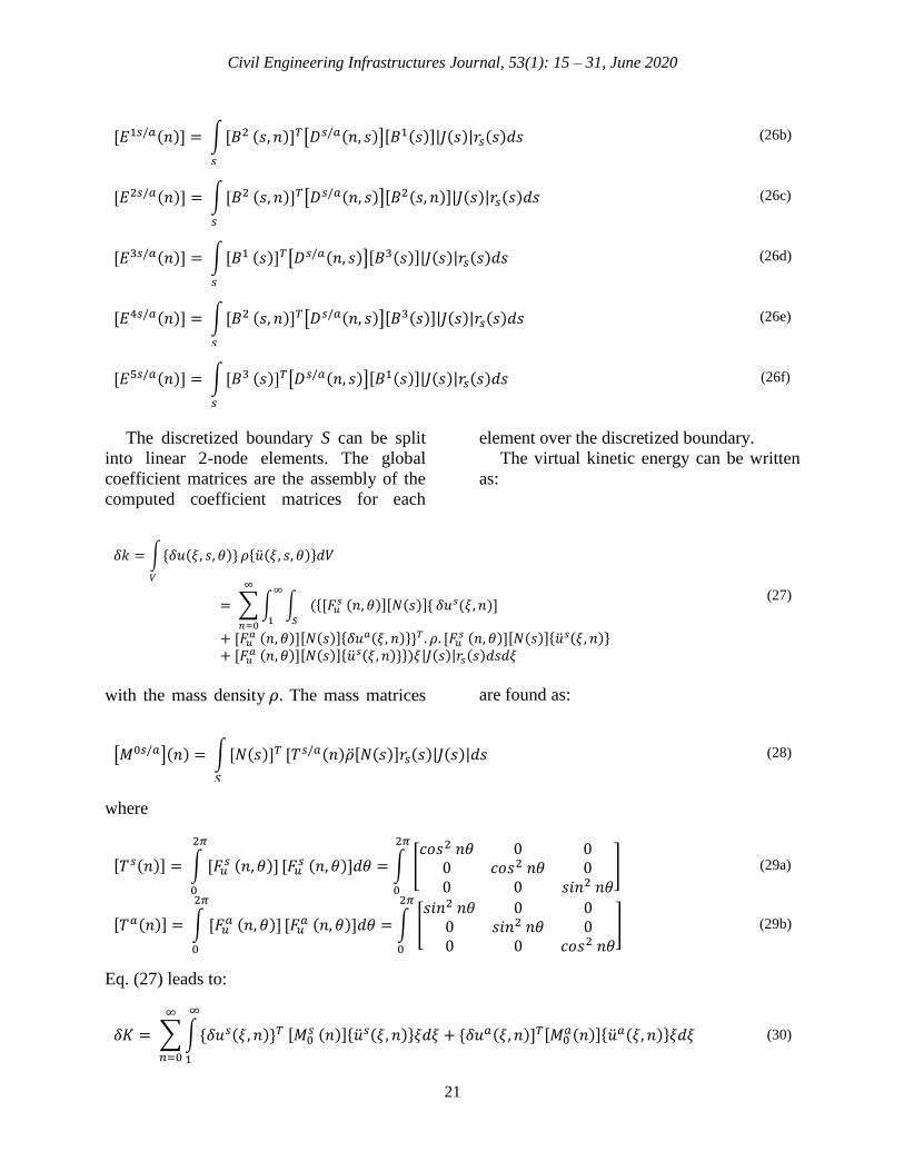
Uniformly Distributed Pressure along the
Depth in Homogenous Material
Consider a hollow unbounded cylinder of
radius 1, thickness 1 and Poisson’s ratio υ =
1/3. The discretization used with one element
of order 10 (Figure 2). Using the Gaussian–
Lobatto–Legendre quadrature for the
numerical integrations alongside the element,
the nodes and integration points match
together. Two cases with free or fixed bottom
have been calculated in the analysis. An
axisymmetric harmonic uniform pressure of
amplitude 1 and in a frequency range of 0 to
10 with 100 steps has been applied in
horizontal direction along the depth and the
displacement of top node due to this loading
has been calculated and compared with the
TLM solution in Figures 3 and 4. Due to the
axisymmetric loading, the computation was
done for the first term of Fourier series (n =
0). The results of the current approach are in
excellent agreement with the TLM.
Fig. 2. Discretization of an unbounded cylinder
Civil Engineering Infrastructures Journal, 53(1): 15 – 31, June 2020
27

Aslmand, M. and Mahmoudzadeh Kani, I.
28
Fig. 3. Real and imaginary displacement of top node due to applied time harmonic pressure (Free bottom)

Civil Engineering Infrastructures Journal, 53(1): 15 – 31, June 2020
29
Fig. 4. Real and imaginary displacement of top node due to applied time harmonic pressure (fixed bottom)
Linearly Varying Pressure along the
Depth in a Homogenous Material
In this example, a linearly antisymmetric
varying pressure of amplitude 1 at the top and
0 at the bottom has been applied in horizontal
direction and the displacement has been
calculated and compared with the TLM
solution in Figure 5. The comparison has
been done for different terms of Fourier series
(n = 0,1,2) along the depth and for 5 layers
discretization (Figure 5). Again the results
match very well with the TLM solutions.
0
0.2
0.4
0.6
0.8
1
1.2
0.0 0.2 0.4
Z (m
)
Displacement (m)
n=0 and ω=0
TLM
AXISBFEM
0
0.2
0.4
0.6
0.8
1
1.2
-0.2 -0.15 -0.1 -0.05 0 0.05
Z (m
)
Displacement (m)
n=0 and ω=3
TLM realAXISBFEM realTLM imaginaryAXISBFEM imaginary

Aslmand, M. and Mahmoudzadeh Kani, I.
30
Fig. 5. The displacement of discretized line for different terms of series (n = 0,1,2) and for different circular
frequencies (ω = 0,3)
CONCLUSIONS
In this paper, an axisymmetric scaled
boundary Finite Element formulation for
elasto-dynamic analysis of three-dimensional
unbounded layered media is derived. The
formulation was based on different terms of
Fourier series and a numerical integration is
required to solve for the dynamic stiffness.
Although the examples presented for the
isotropic case, the current approach is not
restricted to isotropic material. Generally,
anisotropic material can be modeled simply
by modifying the elasticity matrix in
program.
The novel axisymmetric SBFEM
formulation has been validated with the well-
known thin layer method formulation for
different example.
Summarizing, it can be said that the
proposed formulation is very well suited for
the wave propagation of unbounded layered
systems and it could be coupled seamlessly to
a formulation of near field to study the
problem of dynamic soil structure interaction.
ACKNOWLEDGEMENTS
The first author wishes to thank Professor
Carolin Birk and Dr. Hauke Gravenkamp
from the University of Duisburg-Essen. Their
support, encouragement and credible ideas
have been great contributors in the
completion of this research.
REFERENCES
Ardeshir-Behrestaghi, A., Eskandari-Ghadi, M. and
Vaseghi-Amiri, J. (2013). “Analytical solution for
a two-layer transversely isotropic half-space
affected by an arbitrary shape dynamic surface
load”, Civil Engineering Infrastructures Journal,
1(1), 1-14.
Aslmand M., Kani I.M., Birk C., Gravenkamp H.,
0
0.2
0.4
0.6
0.8
1
1.2
0.0 0.2 0.4
Z (m
)
Displacement (m)
n=1 and ω=0
TLMAXISBFEM
0
0.2
0.4
0.6
0.8
1
1.2
-0.4 -0.3 -0.2 -0.1 0
Z (m
)
Displacement (m)
n=1 and ω=3
TLM realAXISBFEM realTLM imaginaryAXISBFEM imaginary
0
0.2
0.4
0.6
0.8
1
1.2
0.00 0.10 0.20 0.30
Z (m
)
Displacement (m)
n=2 and ω=0
TLMAXISBFEM
0
0.2
0.4
0.6
0.8
1
1.2
-0.2 -0.1 0 0.1 0.2Z
(m)
Displacement (m)
n=2 and ω=3
TLM realAXISBFEM realTLM imaginaryAXISBFEM imaginary

Civil Engineering Infrastructures Journal, 53(1): 15 – 31, June 2020
31
Krome F. and Ghadi M.E. (2018). “Dynamic soil-
structure interaction in a 3D layered medium
treated by coupling a semi-analytical axisymmetric
far field formulation and a 3D Finite Element
model”, Soil Dynamics and Earthquake
Engineering, 115, 531-544.
Baidya, D.K., Muralikrishna, G. and Pradhan, P.K.
(2006). “Investigation of foundation vibrations
resting on a layered soil system”, Journal of
Geotechnical and Geoenvironmental Engineering,
132(1), 116-123.
Birk, C. and Behnke, R. (2012). “A modified scaled
boundary Finite Element method for three-
dimensional dynamic soil-structure interaction in
layered soil”, International Journal for Numerical
Methods in Engineering, 89(3), 371-402.
Coulier, P., François, S., Lombaert, G. and Degrande,
G. (2014). “Coupled Finite Element -hierarchical
Boundary Element methods for dynamic soil-
structure interaction in the frequency domain”,
International Journal for Numerical Methods in
Engineering, 97(7), 505-530.
Doherty, J.P. and Deeks, A.J. (2003). “Scaled
boundary Finite-Element analysis of a non-
homogeneous elastic half-space”, International
Journal for Numerical Methods in Engineering;
57(7), 955-973.
Eskandari-Ghadi, M., Hasanpour-Charmhini, A. and
Ardeshir-Behrestaghi, A. (2014). “A method of
function space for vertical impedance function of a
circular rigid foundation on a transversely isotropic
ground”, Civil Engineering Infrastructures
Journal, 47(1), 13-27.
Gazetas, G. (1980). “Static and dynamic displacements
of foundations on heterogeneous multilayered
soils”, Géotechnique, 30(2), 159-177.
Genes, M.C. (2012). “Dynamic analysis of large-scale
SSI systems for layered unbounded media via a
parallelized Coupled Finite Element/ Boundary
Element/ Scaled Boundary Finite Element model”,
Engineering Analysis with Boundary Elements,
36(5), 845–857.
Karabalis, D.L. and Mohammadi, M. (1998). “3-D
dynamic foundation-soil-foundation interaction on
layered soil”, Soil Dynamics and Earthquake
Engineering, 17(3), 139-152.
Kausel, E. and Roesset, J.M. (1975). “Dynamic
stiffness of circular foundations”, Journal of the
Engineering Mechanics Division, 101,771-785.
Krome, F., Gravenkamp, H., and Birk, C. (2017).
“Prismatic semi-analytical elements for the
simulation of linear elastic problems in structures
with piecewise uniform cross section”, Computers
and Structures, 192, 83-95.
Li, B., Cheng, L., Deeks, A.J. and Teng, B. (2005). “A
modified Scaled Boundary Finite-Element method
for problems with parallel side-faces, Part I:
Theoretical developments”, Applied Ocean
Research, 27(4-5), 216-223.
Lysmer, J. and Waas, G. (1972), “Shear waves in plane
infinite structures”, Journal of the Engineering
Mechanics Division, 98(EM1), 85-105.
Morshedifard, A. and Eskandari-Ghadi, M. (2017),
“Coupled BE-FE scheme for three-dimensional
dynamic interaction of a transversely isotropic
half-space with a flexible structure”, Civil
Engineering Infrastructures Journal, 50(1), 95-
118.
Nogami, T., Mahbub, A.A. and Chen, S.H. (2005). “A
new method for formulation of dynamic responses
of shallow foundations in simple general form”,
Soil Dynamics and Earthquake Engineering, 25(7-
10), 679-688.
Rahnema, H., Mohasseb, S. and JavidSharifi, B.
(2016). “2-D soil-structure interaction in time
domain by the SBFEM and two non-linear soil
models”, Soil Dynamics and Earthquake
Engineering, 88(June), 152-175.
Syed, N.M. and Maheshwari, B.K. (2015).
“Improvement in the computational efficiency of
the coupled FEM-SBFEM approach for 3D seismic
SSI analysis in the time domain", Computers and
Geotechnics, 67, 204-212.
Wolf, J.P. (2003). The Scaled Boundary Finite
Element method, John Wiley & Sons: Chichester.
Wolf, J.P. and Preisig, M. (2003). “Dynamic stiffness
of foundation embedded in layered half space
based on wave propagation in cones”, Earthquake
Engineering and Structural Dynamics, 32(7),
1075-1098.
Yaseri, A., Bazyar, M. and Hataf, N. (2014). “3D
Coupled Scaled Boundary Finite Element/Finite
Element analysis of ground vibrations induced by
underground train movement”, Computers and
Geotechnics, 60, 1-8.


