Download - Balkrishna Thesis June 2006 - drs.nio.org


DEPARTMENT OF APPLIED GEOLOGY BARKATULLAH UNIVERSITY BHOPAL-462026 (M.P.)
Dr. D.C. GuptaProfessor & Head Tel: 91-755-2677721 (O)Department of Applied Geology email: [email protected]
Certificate
This is to certify that dissertation entitled “Application of GIS and Remote Sensing
in the analysis of environment of Bay of Bengal” submitted by Mr. Bal
Krishna Patidar from Barkatullah University, Bhopal (M.P.) in partial
fulfillment of the requirement for the award of the degree of Master of Science in
“Geoinformatics” is based on the results of the study carried out by him at NIO, Goa from
1st March to 30th June 2006. It is further certified that this dissertation in full or in parts have
not been previously submitted for the award of any other degree or diploma by any other
candidate.
Date: Dr. D.C. Gupta
Place: Bhopal Professor & Head Department of Applied Geology Barkatullah University, Bhopal

Contents
Page no.
Acknowledgement i
List of Figures iii
List of Tables vi
Chapter 1. General Introduction 1 - 4
1.1 Introduction to Bay of Bengal 1
1.2 Hydrography and Circulation in Bay 1
1.3 Oceanic Environmental Parameters 3
1.3.1 Sea Surface Temperature
1.3.2 Chlorophyll Concentration
1.3.3 Sea Surface Wind
1.3.4 Sea Surface Height
1.4 Statement of Problem and Motivation 4
1.5 Objectives 4
Chapter 2. Introduction to GIS and Remote Sensing 5
2.1 Introduction to GIS 5
2.1.1 Definitions 5
2.1.2 Components of GIS 5
2.1.3 Applications of GIS 7
2.2 GIS for oceanic studies 8

2.3 Introduction to Remote Sensing 10
2.3.1 Definitions
2.3.2 Sensor
2.4 Remote sensing for Oceans 12
2.4.1 Remote Sensing for Chlorophyll Concentration 12
2.4.2 Remote Sensing for Sea Surface Temperature 14
2.4.3 Remote Sensing for Sea Surface Height 15
2.4.4 Remote Sensing for Sea Surface Wind 17
2.5 Integrating Remotely Sensed Data through GIS 18
Chapter 3. Materials and Methodology 19 - 23
3.1 Data Used 19
3.2 Methodology 21
Chapter 4. Result and Discussion 24 - 60
4.1 Seasonal cycle 24 - 40
4.1.1 Seasonal distribution of sea surface temperature 24
4.1.2 Seasonal distribution of chlorophyll concentration 29
4.1.3 Seasonal distribution of sea surface height 34
4.1.4 Seasonal distribution of sea surface wind 38
4.2 Inter-annual cycle 41 - 60
4.2.1 Inter-annual distribution of sea surface temperature 41
4.2.2 Inter-annual distribution of chlorophyll concentration 48
4.2.3 Inter-annual distribution of sea surface height 55
Chapter 5 Summary and Conclusion 61-63
References 64

Acknowledgement
It gives me an immense pleasure in presenting this project report titled “ APPLICATION
OF GIS AND REMOTE SENSING IN ANALYSIS OF ENVIRONMENT OF BAY OF
BENGAL” And I am very thankful to the many mind and hands that cooperated along with
me to make this project of mine a success.
I am very thankful to Dr. D. C. Gupta, Professor and Head, Department of Applied
Geology, Barkatullah University, Bhopal for permitting me to carry out my project work at
National Institute of Oceanography, Goa. His valuable suggestions, inspiration, sound
knowledge of subject and critical evaluation of the investigation result throughout the
academic period has immensely help me for successful completion of my work.
I am very thankful to Dr. S. R. Shetye, Director National Institute of Oceanography, Goa for
permitting me to carry out my project work at NIO, Goa.
It gives me immense satisfaction to express my deep sense of gratitude to my Co-guide
Dr. S. Prasanna Kumar, Deputy Director & Scientist F, Physical Oceanographic Division,
NIO, Goa for their erudite guidance, encouragement, frequent decision, enthusiastic interest
and constructive criticism through all phases of progress for this dissertation work. I believe
that the best way to remember all he has done for me is to work hard in future with that I
have learned from him. Inspite of his busy schedules, he was always ready to spare his time
for me.
I would like to express my sincere thanks to Mr. Andrew Menezes, Scientist, MICD, NIO,
who is my external guide for his constant support and encouragement, for providing me with
the necessary facilities, suggestions and guidance throughout the project work.
i

I would also like to my sincere thanks to Dr. K. K. Rao, Department of Applied Geology,
Barkatullah University, Bhopal for his sound knowledge of subject, guidance and best
teaching throughout my academic period.
I am also grateful to Mr. Rajiv Kumar, Department of Applied Geology, Barkatullah
University, Bhopal for the enthusiasm, great inspiration, sound advice and encouragement
throughout my academic period.
I am thankful to Mr. Pradeep Shrivastava, Staff, Department of Applied Geology,
Barkatullah University, Bhopal for his cooperation and managing the facility during the
course work.
I would also like to thank Mr. A. M. Singh and Mr. Pradeep Sharma for his valuable
suggestions, sound knowledge of subject and a lot of new ideas throughout my academic
period.
I am greatly thanks to Dr. M. Ramaih, Scientist, NIO, Goa and Mr. Gourish Salgaonkar,
Project Assistance, NIO for his valuable suggestions and moral support.
I would like to express my sincere thanks to my classmates Ms. Sapna Godiya, Ms.
Ashlesha Saxena, Mr. Sanjeev Verma, Mr. Devendra Singh Rajput, Ms. Sunita Kumari
and Ms. Versa Waiker for their suggestions and moral support throughout dissertation
period at NIO.
I would also like to thank my other classmates and friends for their suggestions,
encouragement and support and all the help they rendered.
Most of all thanks to GOD the divine who continues make the impossible to possible.
Above all these it is because of my beloved parents who had taken painstaking effort to
bring me up this level and I solemnly place all the credits for this project work at their feet.
ii

LIST OF FIGURES
Figure no. Title Pg. No.
Chapter 2 Introduction to GIS and Remote Sensing
Fig 1. Block diagram showing the component of the GIS 6
Fig.2 Picture showing capability of GIS, which can generate different 9
layers of information about Ocean.
Fig.3 Schematic showing the Data Collection by Remote Sensing 10
Fig. 4 Schematic showing the principle of Radar altimetry 15
Chapter 3 Materials and Methodology
Fig. 5 Flow chart showing various steps followed while processing 22
the Remote Sensing data using GIS Techniques.
Chapter 4 Result and Discussion
Seasonal Cycle
Fig. 6 Monthly mean SST distribution in Bay of Bengal in January 2003 25
Fig.7 Monthly mean SST distribution in Bay of Bengal in April 2003 26
Fig.8 Monthly mean SST distribution in Bay of Bengal in July 2003 26
Fig.9 Monthly mean SST distribution in Bay of Bengal in August 2003 27
Fig.10 Monthly mean SST distribution in Bay of Bengal in October 2003 27
Fig.11 Monthly mean Chlorophyll Pigment Concentration distribution 30
in Bay of Bengal in January 2003
Fig.12 Monthly mean Chlorophyll Pigment Concentration distribution 31
in Bay of Bengal in April 2003
Fig.13 Monthly mean Chlorophyll Pigment Concentration distribution 31
in Bay of Bengal in July 2003
iii

Fig. No. Titles Pg.no.
Fig.14 Monthly mean Chlorophyll Pigment Concentration distribution 32
in Bay of Bengal in August 2003
Fig.15 Monthly mean Chlorophyll Pigment Concentration distribution 32
in Bay of Bengal in October 2003
Fig. 16 Monthly mean SSH distribution in Bay of Bengal in January 2003 35
Fig. 17 Monthly mean SSH distribution in Bay of Bengal in April 2003 36
Fig. 18 Monthly mean SSH distribution in Bay of Bengal in July 2003 36
Fig. 19 Monthly mean SSH distribution in Bay of Bengal in August 2003 37
Fig. 20 Monthly mean SSH distribution in Bay of Bengal in October 2003 37
Fig. 21a Distribution of monthly mean U-component of SSW in April 2003 39
Fig. 21b Distribution of monthly mean V-component of SSW in April 2003 39
Fig. 22a Distribution of monthly mean U-component of SSW in August 2003 40
Fig. 22b Distribution of monthly mean V-component of SSW in August 2003 40
Inter-annual Cycle
Fig. 23 Monthly mean SST distribution in Bay of Bengal in January 2002 42
Fig. 24 Monthly mean SST distribution in Bay of Bengal in January 2003 42
Fig. 25 Monthly mean SST distribution in Bay of Bengal in January 2004 43
Fig. 26 Monthly mean SST distribution in Bay of Bengal in January 2005 43
Fig.27 Monthly mean SST distribution in Bay of Bengal in August 2002 45
Fig.28 Monthly mean SST distribution in Bay of Bengal in August 2003 45
Fig.29 Monthly mean SST distribution in Bay of Bengal in August 2004 46
Fig.30 Monthly mean SST distribution in Bay of Bengal in August 2005 46
iv

Fig. no. Titles Pg. no.
Fig.31 Monthly mean Chlorophyll Pigment Concentration distribution 49
in Bay of Bengal in January 2002
Fig.32 Monthly mean Chlorophyll Pigment Concentration distribution 49
in Bay of Bengal in January 2003
Fig.33 Monthly mean Chlorophyll Pigment Concentration distribution 50
in Bay of Bengal in January 2004
Fig.34 Monthly mean Chlorophyll Pigment Concentration distribution 50
in Bay of Bengal in January 2005
Fig.35 Monthly mean Chlorophyll Pigment Concentration distributio 52
in Bay of Bengal in August 2002
Fig.36 Monthly mean Chlorophyll Pigment Concentration distribution 52
in Bay of Bengal in August 2003
Fig.37 Monthly mean Chlorophyll Pigment Concentration distribution 53
in Bay of Bengal in August 2004
Fig.38 Monthly mean Chlorophyll Pigment Concentration distribution 53
in Bay of Bengal in August 2005
Fig. 39 Monthly mean SSH distribution in Bay of Bengal in January 2002 56
Fig. 40 Monthly mean SSH distribution in Bay of Bengal in January 2003 56
Fig. 41 Monthly mean SSH distribution in Bay of Bengal in January 2004 57
Fig. 42 Monthly mean SSH distribution in Bay of Bengal in January 2005 57
Fig. 43 Monthly mean SSH distribution in Bay of Bengal in August 2002 59
Fig. 44 Monthly mean SSH distribution in Bay of Bengal in August 2003 59
Fig. 45 Monthly mean SSH distribution in Bay of Bengal in August 2004 60
Fig. 46 Monthly mean SSH distribution in Bay of Bengal in August 2005 60
V

LIST OF TABLES
Table no. Title Pg. No.
Table 1 Characteristic of SeaWiFS 13
Table 2 Characteristics of MODIS 14
Table 3 Details pertaining to the remote sensing data used for 20
the study including sensor, resolution and data source.
Table 4 Basin averaged SST with its maximum and minimum 28
value during different months in the year 2003
Table 5 Basin averaged chlorophyll pigment concentrations with 33
its maximum and Minimum value during different
months in the year 2003
Table 6 Summarizes the basin-wide average SST during January 47
and August of each year from 2002 to 2005.
Table 7 Basin averaged chlorophyll pigment concentrations with 54
its maximum and minimum value during January and
August of each year from 2002 to 2005.
Vi


CHAPTER 1
General Introduction
1.1 Introduction to Bay of Bengal
The Bay of Bengal is a northern extended arm of the Indian Ocean, which occupies almost 2.2
million sq km area between equator and 220N latitude and 800E and 1000E longitudes. It is
bounded in the west by the east coasts of Sri Lanka and India, on the north by the deltaic region
of the Ganges-Brahmaputra-Meghna river system, and on the east by the Myanmar peninsula.
The southern boundary of the Bay is approximately along the line drawn from Dondra Head in
the south of Sri Lanka to the north tip of Sumatra. A broad U-shaped basin characterizes the
bottom topography of the Bay of Bengal with its south opening to the Indian Ocean. A thick
uniform abyssal plain occupies almost the entire Bay of Bengal gently sloping southward at an
angle of 8°-10°. In many places underwater valleys dissect this plain mass. The Bay of Bengal
plays an important role in the climatic conditions of the adjacent land regions such as India,
Bangladesh, Myanmar, Indonesia and Sri Lanka. The information about the seawater of the
Bay of Bengal and its characteristics and circulation along the coast has paramount importance
in understanding the numerous ocean processes. In the Bay of Bengal, the physical, chemical
and biological processes are linked in an intimate manner. Oceanic environmental features such
as Sea surface temperature, Sea surface wind and Chlorophyll concentration are important in
assessing productivity of Bay of Bengal. The chlorophyll concentration is found to be
dependent on the sea surface temperature, wind and monsoon activities.
1.2 Hydrography and circulation in Bay of Bengal
Hydrography and circulation of the Bay of Bengal is basically determined by the monsoon
wind, which reverses semi-annually. The Bay of Bengal is forced locally by seasonally
reversing monsoon winds and remotely by the winds in the equatorial Indian Ocean (McCreary
et al., 1993). During the summer monsoon (June to September) the southwesterly winds of
oceanic origin blows over the Bay of Bengal with very high speed (10-15m/s). During winter
monsoon (November to February) the northeasterly winds of dry continental origin blows over
1
the Bay with speed of about 5 m/s. In spring (March-May) and fall (October), the winds are
generally weak and variable. In response to these reversing winds the circulation of the Bay of
Bengal also changes its direction. Surface circulation is found to be generally clockwise from
January to July and counter-clockwise from August to December, in accordance with the
reversible monsoon wind systems. The circulation in the Bay of Bengal is characterized by
anticyclonic flow during most months and strong cyclonic flow during November. The flow is
not constant and depends on the strength and duration of the winds. During the Southwest
monsoon season, currents in the entire bay are weak and consists of several circulation features
like eddies, meanders etc.
The Bay of Bengal receives a large quantity of fresh water from both rainfall and river runoff
from the bordering countries. Annually, the major rivers Irrawaddy, Brahmaputra, Ganga and
Godavari discharge about 1.5X10¹² m3 of fresh water into the Bay of Bengal and rainfall ranges
between 1m and 3m (Shetye et al., 1996). Fresh water from the rivers largely influences the
coastal northern part of the Bay. The rivers of Bangladesh discharge the vast amount of 1,222
million cubic meters of fresh water (excluding evaporation, deep percolation losses and
evapotranspiration) into the Bay. The temperature, salinity and density of the water of the
southern part of the Bay of Bengal is, almost the same as in the open part of the ocean. In the
coastal region of the Bay and in the northeastern part of the Andaman Sea where a significant
influence of river water is present, the temperature and salinity are seen to be different from the
open part of the Bay. Thus, the circulation and hydrography of the Bay of the Bengal is
complex due to the interplay of the semi-annually reversing monsoon winds and the associated
heat and large amount of freshwater fluxes from rivers. A unique feature of the Bay is
occurrence of cyclones during October-November and April-May.
1.3 Oceanic environmental parameters
1.3.1 Sea Surface Temperature (SST)
Sea surface temperature (SST) is the water temperature at 1meter below the sea surface. The
physical property that can be measured with relative ease is the sea surface temperature. It is
the most important oceanic parameter for both meteorologists and oceanographers because of
its significant role in the exchange of heat, moisture and gases across the air-sea interface.
2

SST is indicative of ocean surface process - features like upwelling, fronts, eddies and current
boundaries, etc. SST is primarily affected by the energy transfer process at the air-sea boundary
and advection in the oceanic surface layer. The distribution of temperature in any region of sea
or ocean is determined by the fluxes of heat through the sea surface and exchanges of heat, by
advection or eddy diffusion, with the water of adjacent regions.
1.3.2 Chlorophyll Concentration
Chlorophyll-a concentration is an indicator of the phytoplankton biomass in the sea and is
responsible for the photosynthesis. Chlorophyll-a concentration in the ocean can be estimated
from the radiance detected in a set of suitably selected wavelengths through a retrieval
procedure.
1.3.3 Sea Surface Wind
Sea surface wind determines the sea surface roughness and wave climate and thereby play
significant role in the energy exchange at the air-sea interface. Sea surface winds drive the
circulation of the upper ocean. The wind driven circulation is principally in the upper few
hundreds meters and therefore is primarily a horizontal circulation in contrast to the
thermohaline one.
1.3.4 Sea Surface Height
Sea surface height is defined as the distance of the sea surface above the referenced ellipsoid.
The SSH computed from altimeter range and satellite altitude above the referenced ellipsoid.
Sea surface height often shown as a sea surface anomaly or sea surface deviation, this is
difference between the SSH at the time of measurement and the average SSH for that region
and time of year. The variable height of the sea surface above or below the geoid.
3

1.4 Statement of problem and motivation
The Bay of Bengal is traditionally considered to be low productive region. Since the fisheries
of a region is closely related to the chlorophyll and biological productivity, it is important to
understand the distribution of chlorophyll and what controls it. The Bay of Bengal is the least
explored region in the Indian Ocean and very few studies have attempted to analyze the
satellite derived chlorophyll pigment concentrations. This is the motivation for this dissertation
work, which aims at understanding the distribution and variability of the chlorophyll
concentrations along with other environmental parameters.
1.5 Objectives
The main objective of this study is to use the GIS and remote sensing tools for analysis of the
oceanic parameters in the Bay of Bengal.
The specific objectives of this study are:
1) To analyze the seasonal and inter-annual distribution and variability of chlorophyll pigment
concentration of Bay of Bengal using GIS and remote sensing.
2) To analyze the seasonal and inter-annual distribution and variability of SST, SSH and SSW.
3) To analyze the correlation between chlorophyll concentration and others parameters such as
SST, SSH and Wind, where these are related.
4


CHAPTER 2
INTRODUCTION TO GIS AND REMOTE SENSING
2.1 Introduction to GIS
2.1.1 Definitions
A Geographic Information Systems (GIS) is a computer system for managing spatial data.
The word geographic implies that location of the data items are known in terms of
geographic coordinates (latitude, longitude). The word information implies that the data in a
GIS are organized to yield useful knowledge, often as colored maps and images, but also as
statistical graphics, tables, and various on-screen responses to interactive queries. The word
system implies that a GIS is made up from several interrelated and linked components with
different functions. Thus, GIS have functional capabilities for data capture, input,
manipulation, transformation, visualization, combination, query, analysis, modeling and
output. A GIS consists of a package of computer programs with a user interface that provides
access to particular functions.
We can define the GIS in following words:
“GIS is a collection of computer hardware, software, and geographic data for capturing,
managing, analyzing, and displaying all forms of geographically referenced information.”
In other words GIS as, "a computer based system that provides four sets of capabilities to
handle geo-referenced data:
1. Data input
2. Data management (data storage and retrieval)
3. Manipulation and analysis
4. Data output.
2.1.2 Components of GIS
GIS constitutes of five key components:
Hardware, Software, Data, People and Procedure.
Figure1 showing the block diagram of component of the GIS.
5

Figure1 Block diagram showing the component of the GIS
Hardware
GIS requires specialized hardware devices. Hardware capabilities affect processing speed,
ease of use and the type of output available.
Software
GIS software provides the functions and tools needed to store, analyze, and display
geographic information. GIS softwares in use are ARC/GIS, ARC/View, MapInfo, ARC/Info,
AutoCAD Map, etc. software includes not just the GIS software, but also the various
database, drawing, statistical, imaging, or other specific application software.
6

Data
The availability and accuracy of data can affect the results of any query or analysis.
People
People are the most important component of GIS. People are required to develop procedures
and define the tasks of GIS. People can often overcome shortfalls in other components of the
GIS, but the opposite is not true.
Procedure
Analysis requires well-defined, consistent, methods to produce correct and reproducible
results.
2.1.3 Applications of GIS
Computerized mapping and spatial analysis have been developed simultaneously in several
related fields. The present status would not have been achieved without close interaction
between various fields such as utility networks, cadastral mapping, topographic mapping,
thematic cartography, surveying and photogrammetery remote sensing, image processing,
computer science, rural and urban planning, earth science, and geography and Oceanography.
We can use GIS technology in many fields such as:
Forestry
Natural Hazards
Disaster Management
Oceanography
Environmental Study
Geology
Land use/ Land Cover Analysis
Urbanization
Rural Development
Infrastructure and Utilities
Health and Healthcare
Business Marketing and Sales etc
7

2.2 GIS for the Oceanic Studies
Applications of GIS technology in the various oceanographic disciplines are multifaceted.
They deal with data acquired with a variety of different methods and integration principles
from different technological disciplines in an attempt to facilitate the resolution of the
dynamics of the marine environment. Oceanographic GIS purpose solution to an ever-
increasing number of marine problems and at the same time provide new insights to the
unknown abyssal depths of our oceans. Ocean dynamics (oceanographic processes) as well
as marine problems have inherent spatiotemporal characteristics. Oceanographic data have
two essential parts (location and attributes) that makes them highly suitable for input to
geospatial databases, which in turn open new ways for data storage, analysis and
visualization. The majority of oceanographic data often have a geographic location, are
digital. The spatial attribute of oceanographic data makes them highly suitable for GIS
analysis as GIS provides a natural framework for the acquisition, storage, and analysis of
georeferenced data. GIS database can store and manipulate oceanic datasets of several
environmental parameters about physical, chemical, biological ocean process and present
their effects on the marine environment in graphical format. Scientists, academics, and
professionals studying the world’s oceans and seas use Geographic Information Systems
(GIS) to investigate their areas of interest. In recent years, the applications of GIS increased
in the studies of oceanic process. Applications of GIS technology are used in a variety of
ways, such as distribution tools, mapping tools and monitoring analysis tools and in a variety
of disciplines, such as ocean surface processes, environmental and bioeconomic
charaterisation of coastal and marine system, fisheries, sea level rise and climate change,
marine geology and geomorphology, coastal zone assessment and management, deep ocean
mapping etc.
Compared to land-based sciences, regarding terms of mapping, managing and modeling,
based on spatial data, Geographic Information systems (GIS) are not widely used in marine
sciences of the pelagic and deep ocean. The volume of data collected from oceans through
remote sensing and acoustic as well as traditional field observation techniques has become
tremendously large and complex.8

The interdisciplinary nature of studying marine processes requires data integration of multiple
types and formats. Despite large variations, all the data share the common characteristic of
physical location. This georeferencing feature allows the integration of data from all sources
and types under a single platform, a geographic information system. See Figure 2.
Figure 2 Picture showing capability of GIS, which can generate different
layers of information about Ocean.
9

2.3 Introduction to Remote Sensing
2.3.1 Definitions
We can define the remote sensing in following words:
"Remote sensing is the science (and to some extent, art) of acquiring information about the
Earth's surface without actually being in contact with it. This is done by sensing and recording
reflected or emitted energy and processing, analyzing, and applying that information."
Electro-magnetic radiation, which is reflected or emitted from an object, is the usual source of
remote sensing data. However any media such as gravity or magnetic fields can be utilized in
remote sensing. The characteristics of an object such as temperature, height, and chlorophyll
concentration etc. of ocean can be determined, using reflected or emitted electro-magnetic
radiation, from the object. That is, "each object has a unique and different characteristics of
reflection or emission if the type of object or the environmental condition is different.” Remote
sensing is a technology to use for identifies and understands the characteristics or the
environmental condition of the ocean through the uniqueness of the reflection or emission. See
Figure 3.
Figure 3 Schematic showing the Data Collection by Remote Sensing
10
Remote sensing is classified into three types with respect to the wavelength regions:
(1) Visible and Reflective Infrared Remote Sensing,
(2) Thermal Infrared Remote Sensing and
(3) Microwave Remote Sensing
The energy source used in the visible and reflective infrared remote sensing is the sun. Remote
sensing data obtained in the visible and reflective infrared regions mainly depends on the
reflectance of objects on the ground surface. Therefore, information about objects can be
obtained from the spectral reflectance.
The source of radiant energy used in thermal infrared remote sensing is the object itself,
because any object with a normal temperature will emit electro-magnetic radiation with a peak.
In the microwave region, there are two types of microwave remote sensing, passive microwave
remote sensing and active remote sensing. In passive microwave remote sensing, the microwave
radiation emitted from an object is detected, while the back scattering coefficient is detected in
active microwave remote sensing.
2.3.2 Sensor A device to detect the electro-magnetic radiation reflected or emitted from an object is called a
"remote sensor" or "sensor". Cameras or scanners are examples of remote sensors. A vehicle to
carry the sensor is called a "platform". Aircraft or satellites are used as platforms.
We can divide the sensor in two types - Passive Sensor and Active Sensor.
Passive sensors detect the reflected or emitted electro-magnetic radiation from natural sources,
while active sensors detect reflected responses from objects, which are irradiated from
artificially, generated energy sources, such as radar.
Each is further divided in to non-scanning and scanning systems.
A sensor classified as a combination of passive, non-scanning and non-imaging method is a type
of profile recorder, for example a microwave radiometer. A sensor classified as passive, non-
scanning and imaging method, is a camera, such as an aerial survey camera or a space camera,
for example on board the Russian COSMOS satellite.
11

Sensors classified as a combination of passive, scanning and imaging are classified further into
image plane scanning sensors, such as TV cameras and solid state scanners, and object plane
scanning sensors, such as multispectral scanners (optical-mechanical scanner) and scanning
microwave radiometers. An example of an active, non-scanning and non-imaging sensor is a
profile recorder such as a laser spectrometer and laser altimeter. An active, scanning and imaging
sensor is radar, for example synthetic aperture radar (SAR), which can produce high resolution,
imagery, day or night, even under cloud cover.
2.4 Remote sensing for Oceans
Remote Sensing is a technique based on measuring the electromagnetic energy reflected or
emitted by the surface of geographic space (Caloz and Collet, 2003). Satellites are able to sense
an array of parameters including ocean color, Sea Surface Temperature, Sea Surface Height
Anomalies and Sea Surface winds (Simpson, J.J. 1992). Remote Sensing data provides Sea
surface temperature information along with data on sea surface height and also provides
information on the oceanic and atmospheric phenomena, chlorophyll concentration, sea surface
wind etc. Remote sensing of the ocean environment comprises the greatest source of information
about several oceanic environmental parameters of the ocean surface. Remote sensing monitoring
provides important tools for better understanding of the marine processes, ecology and the ocean
environmental changes. The most widely used remote sensing techniques today are based on the
detection/sensing of electromagnetic radiations. Remote sensing of oceanic parameter from space
provide advantage point from which maps of oceanic properties on a very large scale can be
prepared. Remote sensing techniques is a very useful tool for synoptic and continuous study of
oceanic parameters over Bay of Bengal.
2.4.1 Remote Sensing for Chlorophyll Concentration
Satellite ocean color remote sensing is based on sensing the radiance exiting the ocean surface
that contains a wealth of spectral information regarding the absorption and scattering processes of
the constituents within the water column that include water itself, phytoplankton, colored
dissolved organic matter, and suspended sediments (Kirk, 1994). The goal of remote sensing of
ocean color is to derive quantitative information on the types and concentrations of these
12
substances present in the water from variations in spectral form and magnitude of the emergent
flux from the ocean. Ocean color is determined by remote sensing reflectance (Rrs); the ratio of
water leaving radiance (Lu) to down welling irradiance (Kirk, 1994). It is a measure of how much
of the down welling light that is incident onto the water surface is eventually returned through the
surface and is a product of the specific absorption spectra of the water column constituents. Most
commonly, ocean color information is used to determine chlorophyll concentration that is used as
a proxy for phytoplankton biomass. This information is then used to quantitatively determine the
ocean’s role in biogeochemical cycles, determine the magnitude and variability of primary
production, and timing of phytoplankton blooms. However, current progressive research is also
trying to discern many other parameters from ocean color revealing information about suspended
sediments, organic matter concentrations, coccolith concentration, various pigment
concentrations, attenuation of light, total absorption, and chlorophyll fluorescence which is used
as a proxy for phytoplankton physiological stress.
SeaWiFS for Chlorophyll Concentration
The purpose of the Sea-viewing Wide Field-of-view Sensor (SeaWiFS) Project is to provide
quantitative data on global ocean bio-optical properties to the Earth science community. Subtle
changes in ocean color signify various types and quantities of marine phytoplankton
(microscopic marine plants), the knowledge of which has both scientific and practical
applications.
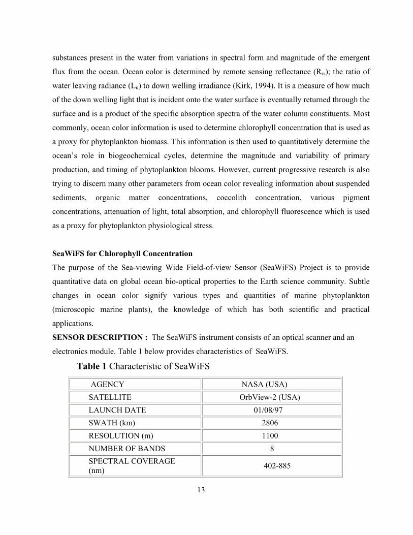
SENSOR DESCRIPTION : The SeaWiFS instrument consists of an optical scanner and an
electronics module. Table 1 below provides characteristics of SeaWiFS.
Table 1 Characteristic of SeaWiFS
AGENCY NASA (USA)
SATELLITE OrbView-2 (USA)
LAUNCH DATE 01/08/97
SWATH (km) 2806
RESOLUTION (m) 1100
NUMBER OF BANDS 8
SPECTRAL COVERAGE (nm)
402-885
13

2.4.2 Remote Sensing for Sea Surface Temperature
Satellite remote sensing can provide thermal information in a short time over a wide area.
Temperature measurement by remote sensing is based on the principle that any object emits
electro-magnetic energy corresponding to the temperature, wavelength and emissivity.
MODIS for Sea Surface Temperature
MODIS (Moderate Resolution Imaging Spectroradiometer) is key instrument aboard the Terra
(EOS AM) and Aqua (EOS PM) satellites. Terra’s orbit around the earth is timed so that it passes
from north to south across the equator in the morning, while Aqua passes south to north over the
equator in the afternoon. Terra MODIS and Aqua MODIS are viewing the entire Earth's surface
every 1 to 2 days, acquiring data in 36 spectral bands, or groups of wavelengths. See Table 2 for
the characteristics of MODIS. These data will improve our understanding of global dynamics and
processes occurring on the land, in the oceans, and in the lower atmosphere. MODIS is playing a
vital role in the development of validated, global, interactive Earth system models able to predict
global change accurately enough to assist policy makers in making sound decisions concerning
the protection of our environment. This Level 2 and 3 products provide sea surface temperature
at 1-km (Level 2) and 4.6 km, 36 km, and 11(Level 3) resolutions over the global oceans. Table
2 gives showing the characteristics of MODIS.
Table 2 Characteristics of MODIS
Orbit 705 km, sun-synchronous, near-polar, circular
Swathdimensions
2300 km at 110° (±55°) from705 km altitude
Spatialresolution
250 m (bands 1-2) 500 m (bands 3-7) 1000 m (bands 8-36)
14

2.4.3 Remote sensing for Sea Surface Height
One of the ways remote sensing can be used in studying the ocean is by depicting sea surface
height anomalies. Sea surface height anomalies are the difference between the observed and the
average sea surface height as observed by the TOPEX satellite.
Principles of altimeterThe radar altimeter sends short pulses of microwave energy toward the ocean below; the round-
trip travel time of the reflected pulse yields the distance between the spacecraft and the sea
surface. In addition, the shape of the reflected pulse is used to determine wave height and sea-
surface wind speed. See Figure 4.
Figure 4 Schematic showing the principle of Radar altimetry
15

The sea surface height is computed from altimeter range and satellite altitude above the reference
ellipsoid. Sea surface height is often shown as a sea-surface anomaly or sea-surface deviation,
this is the difference between the sea surface height at the time of measurement and the average
sea surface height for that region and time of year. The higher the sea surface height anomaly, the
warmer the layer of water. The ground height or the sea surface height is measured from the
reference ellipsoid. If the altitude of the satellite Hs is given as the height from the reference
ellipsoid, the sea surface height HSSH is calculated as follows.
HSSH = Hs - Ha where, Ha- measured distance between satellite and the sea surface.
The sea surface height is also represented by the geoid height Hg that is measured between the
geoid surface and the reference ellipsoid and the sea surface topography DH.
TOPEX/POSEIDON Altimeter Sensor/Instrument and ERS-1
TOPEX/POSEIDON is a satellite mission that uses radar altimetry to make precise
measurements of sea level with the primary goal of studying the global ocean circulation. ERS-1
is not as accurate an altimetric satellite as TOPEX, but it has been used for important studies
nevertheless. ERS-1 has a much finer spatial resolution (3/4 by 3/4 degree) than
TOPEX/POSEIDON (3 by 3) and a much greater spatial coverage than its more modern
counterpart. This has led ERS-1 to be used to determine tidal components that has been used to
compute the SSH using TOPEX/POSEIDON. The greater spatial coverage with lesser SSH
resolution has led to a technique that calibrates the ERS-1 data with TOPEX. These results are
then meshed and used to obtain a final merged SSH product. The primary science goal of the
TOPEX/POSEIDON mission is to substantially increase our understanding of global ocean
dynamics by making precise and accurate observations of sea level for several years.
TOPEX/POSEIDON will obtain measurements of global ocean surface topography with a
precision of two centimeters and a single-pass accuracy of 13 centimeters along a fixed grid
every ten days for a period of three years.
16

2.4.4 Remote Sensing for Sea Surface Wind
Winds are measured with a microwave radar scatterometer where a radar signal is transmitted to
the surface of the ocean and then is backscattered to the sensor. The roughness of the sea surface
influences to strength of the signal and is used to determine the relative direction and speed of
wind acting on the surface of the ocean. This information is used in air-sea interaction research,
climate research, hurricane forecasting, and ocean circulation. Sea surface irradiance is
determined from atmospheric parameters that determine the amount of sunlight that reaches to
surface of the ocean and is an important factor in climate and also primary production studies.
QuikSCAT/SeaWinds
SeaWinds is a rotating scatterometer (measurement of the surface wind speed and direction over
the ocean) onboard QuikSCAT, launched by NASA in 19th of June 1999. The SeaWinds
instrument on the QuikSCAT satellite is specialized microwave radar that measures near-surface
wind speed and direction under all weather and cloud conditions over Earth's oceans.
Description
Launch Vehicle: Titan II
Orbit: Sun-synchronous, The satellite altitude is about 800 km, 98.6° inclination orbit.
Swath is 1800 km large for the outer beam and 1414 km for the inner beam.
Measurements
1,800-kilometer swath during each orbit provides approximately 90-percent coverage of Earth's
oceans every day.
Wind-speed measurements of 3 to 20 meters/second, with an accuracy of 2 meters/second;
direction, with an accuracy of 20 degrees.
Wind vector resolution - 25 kilometers.
17

2.5 Integrating Remotely Sensed Data through GIS
Remotely sensed data, especially satellite data, is in a ready made spatial data format for GIS.
Thus, it plays a very important role in the optimum utilization of GIS technology. Merging these
two technologies i.e. Remote Sensing and GIS, can results in a tremendous increase in
information for many kinds of users. Remote sensing data, thus, bears a synergistic relationship
to GIS technology and undoubtedly will be a major source of both original and monitoring
information on the earth and ocean’s environment. GIS is the most appropriate framework for the
merging of these data sets on chlorophyll concentration, SST, SSH and SSW. GIS offers a
perfect platform to integrate remotely sensed point data sets. It is a computerized tools and fully
integrated environment designed to acquire, manage, process and analyze spatial information
(Caloz and Collet, 1997). This allows easy investigations of co-relations of variables and
historical and current data can be merged to create a multi-dimensional data set of location, value
and time which leads to inquires based upon location, condition, trends, patterns and modeling
(Lehmann and Lachavanne, 1997). GIS contributes a new dimension to the modeling of
geographic space from a connection to relational or object oriented databases (Caloz and Collet,
1997). GIS is a rich and powerful means of data management, archiving, distribution and
analysis.
18


CHAPTER 3
Materials and Methodology
The main objectives of this study to evaluate the environmental conditions of Bay of Bengal
and analyze the seasonal and inter-annual distribution and variability of oceanic environmental
parameters such as sea surface temperature (SST), chlorophyll concentration, sea surface height
(SSH) anomalies and sea surface wind (SSW) using GIS technology. For the present study
remotely sensed data from different satellites were used to study the environmental
characteristics of the Bay of Bengal. These Remote sensing data were further used for the
analysis in GIS environment.
Data Used
The study domain is from equator to 22oN latitude and 78oE to 100oE longitude. For present
study we used satellite remote sensing monthly mean data on SST, chlorophyll pigment
concentration, sea surface winds and sea surface height anomaly from January 2002 to
December 2005. These datasets we obtained from different sensors. Table 3 gives the details
pertaining to each of the data used in this study.
Data sets:
Sea Surface Temperature (SST)
Chlorophyll Concentration
Sea Surface Height (SSH) Anomaly
Sea Surface Wind (SSW)
19

Table 3 Details pertaining to the remote sensing data used for the study including sensor, resolution and data source.
Serial
no.
Parameter Sensor Resolution Web site
1 Sea surface
temperature
(SST)
Modis Aqua Monthly data at
0.33 degree
resolution
http://oceancolor.gsfc.nasa
.gov/,
http://poet.jpl.nasa.gov/
2 Chlorophyll
pigment
concentration
SeaWifs (Sea
Viewing wide
field of view
sensor)
Monthly data at
0.33 degree
resolution
http://reason.gsfc.nasa.gov
/OPS/Giovanni/ocean.sea
wifs.shtml
3 Sea surface
wind
Quikscat (Quick
Scatterometer)
Daily wind data at
0.25 degree spatial
resolution
http://www.ssmi.com/qsca
t/qscat_browse.html,
http://poet.jpl.nasa.gov/
4 Sea surface
height (SSH)
anomalies
Topex/Posidon
and ERS-1/2
satellites
7-day snap-shots of
the merged sea-
level anomalies at
0.33 degree
resolution
http://las.aviso.oceanobs.c
om
20

Methodology
Once the monthly mean data were extracted, further processing was carried out using GIS
environment. The present work has been carried out in GIS environment using Arc GIS 9.0
and Arc View 3.2 are the GIS software. In general, the processing using GIS can be divided
into three parts - data conversion, contour map generation and analysis.
1. Data conversion - In this step, Remotely sensed ASCII data is first converted in the dbf
format for the GIS environment analysis using MS Access and MS Excel.
2. Contour Map Generation – Subsequently, point map (shape files) of each of the 4
parameters such as sea surface temperature, chlorophyll concentration, sea surface
height and sea surface wind, were prepared in Arc/View 3.2 from the tabular point data.
Then these point maps were called in Arc/GIS for creating contour maps for further
analysis. Then an inverse distance weighting interpolation methods was used for the
creation of filled contour maps of all the parameters.
Inverse Distance Weighted
IDW is an exact interpolator, where the maximum and minimum values in the interpolated
surface can only occur at sample points. To predict a value for any unmeasured location, IDW
will use the measured values surrounding the prediction location. It weights the points closer to
the prediction location greater than those farther away, hence the name inverse distance
weighted. IDW is very suitable for creating filled contour maps that shows the polygon shape
of the datasets.
Filled Contour Map
Filled contour is the polygon representation of the geostatistical layer. It is assumed for the
graphical display that the values between each contour line are the same for all locations within
the polygon. In filled contour every polygon has the minimum and maximum values of the
generated maps.
3. Analysis - In this part, we analyzed the inter-annual and seasonal distribution and
variability of oceanic parameters of Bay of Bengal using filled contour maps of these
parameters and discussed the correlation between these parameters.
21

Remote Sensing Techniques for data
SST from ModisAqua/Terra
SSH from Topex/Posidonand ERS-1/2
SSW from Quikscat
ChlorophyllConcentrationfrom SeaWifs
Data conversion for GIS Environment
GIS Environment
ARC/View 3.2a
Environmental Studiesof Bay of Bengal
Creating point map Creating surface area ofBay of Bengal
ARC/GIS 9.0
Continue
22

Export to Vector format
Create Filled Contour maps of SST, SSH, SSW and Chlorophyll Concentration
Contour Map Generation
Analysis
Inter-annual Variation and distribution Seasonal Variation and distribution
Results and Discussion
Analysis the Correlation between these parameters
Create the IDW maps from shape files of point datausing Inverse Distance Weighting Method
Figure 5 Flow chart showing various steps followed while processing the Remote
Sensing data using GIS Techniques.
23


CHAPTER 4
Results and discussion
Seasonal Cycle
To understand the seasonal cycle, we choose the monthly mean data for the months January,
April, July, August, and October for the year 2003.
Seasonal cycle of sea surface temperature
Sea surface temperature distribution in January showed a pattern, which was uniform in the
zonal direction, but varied meridionally (Fig.6) SST was coldest in the north with the
minimum of 22oC and increased steadily towards south where the maximum was 31oC. In
western bay average SST was seen about 26oC, while in the eastern Bay, it was about 28oc. In
April, the SST showed a rapid heating of 3 to 6oC in the northern Bay compared to winter
(Fig.7). Spatially it varied only marginally from 29oC to 31oC in the entire Bay, expect in
small pockets along the eastern boundary where it was 32oC and in the northern most coastal
region where it was 28oC. By July, as the summer monsoon sets in the Bay, the SST was
more or less uniform in the entire Bay with a value of 29oC (Fig.8). However, SST of 30oC
was noticed in the southwestern and southern region, while 31oC was seen in the southeastern
region. Pockets of colder waters with SST 28oC were seen in the central and eastern Bay. In
August, the SST pattern remains more or less similar to July, except the occurrence of colder
waters around Sri Lanka and northeastern Bay intruding into the central Bay (Fig.9). In
October, in the northern Bay SST was warmest of all the months with a value of 31oC. Entire
Bay was very warm with SST of 30oC, except in a zonal patch in the south and a small pocket
near the western boundary, which was 1oC colder (Fig.10). The distribution pattern of SST
during October was just reverse of that during January. See Table 4 for the basin-averaged
SST for each of the above-discussed month along with the minimum and maximum values.
24

Sea Surface Temperature (oC) Map of Bay of Bengal
Fig.6 Monthly mean SST (oC) distribution in Bay of Bengal in January 2003
25

Fig.7 Monthly mean SST (oC) distribution in Bay of Bengal in April 2003
Fig.8 Monthly mean SST (oC) distribution in Bay of Bengal in July 2003
Sea Surface Temperature (oC) Map of Bay of Bengal
Sea Surface Temperature (oC) Map of Bay of Bengal
26

Fig.9 Monthly mean SST (oC) distribution in Bay of Bengal in August 2003
Sea Surface Temperature (oC) Map of Bay of Bengal
Sea Surface Temperature (oC) Map of Bay of Bengal
Fig.10 Monthly mean SST (oC) distribution in Bay of Bengal in October 2003
27
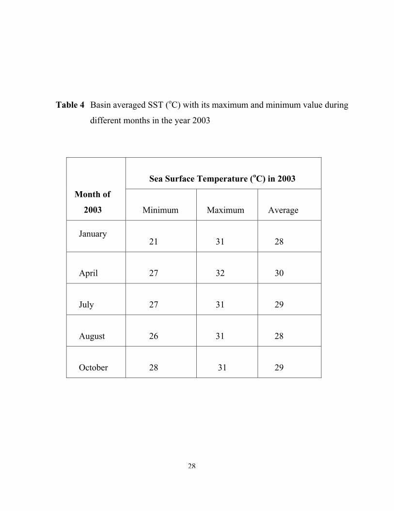
Table 4 Basin averaged SST (oC) with its maximum and minimum value during
different months in the year 2003
Sea Surface Temperature (oC) in 2003
Month of
2003 Minimum Maximum Average
January 21 31 28
April 27 32 30
July 27 31 29
August 26 31 28
October 28 31 29
28

Seasonal cycle of chlorophyll pigment concentration
The distribution of chlorophyll pigment concentration in January varied marginally from 0.1 to
0.3 mg/m3 in the Bay except very close to the coast (Fig.11). Near the coastal areas
chlorophyll pigment concentrations showed large variations from 0.4 to 10 mg/m3. Higher
values of chlorophyll concentration of about 5 to 10mg/m3 were seen near the Ganges-
Brahmaputra-Meghna rivers deltaic region in the north and Irrawady river basin in the eastern
coastal region. One needs to be cautious in interpreting the values very near the coast due to
the possible contamination of signal by sediment load. In April, chlorophyll concentration was
the least in the open Bay with values between 0.1 and 0.2 mg/m3 (Fig.12). As in the case of
January, the concentrations increased rapidly towards the coastal region with a maximum value
of 5 mg/m3, except in 3 small patches near the river mouths of Irrawady, Ganges and Godavari
where the values were as high as 10 mg/m3. In July we see an increase in pigment
concentrations all along the coastal and near shore regions, especially in the Indo-Sri Lanka
region and off Godavari and Krishna rivers where concentrations varied between 2 to 5 mg/m3
(Fig.13). In fact an overall increase in pigment concentrations compared to April was noticed
towards the western and southern Bay of Bengal. In August chlorophyll concentrations were
the highest in the Bay with open sea values between 0.2 to 0.3 mg/m3, while along the western
and northern boundary extending up to the central Bay, the concentrations ranged from 0.4 to
10 mg/m3 (Fig.14). Interesting observation is the extending patch of high chlorophyll
concentrations from Indo-Sri Lanka region towards east into the central Bay. Similarly patch of
high concentration extends from Godavari and Ganges mouth into offshore region. In October,
though the chlorophyll concentrations were high, they were in general less compared to August
(Fig.15). Chlorophyll concentrations in the Indo-Sri Lanka region still remain one of the
highest. Table 5 shows the basin-averaged chlorophyll pigment concentrations for each of the
above-discussed month along with the minimum and maximum values.
29

Chlorophyll Concentration (mg/m3) Map of Bay of Bengal
Fig.11 Monthly mean chlorophyll concentration (mg/m3) distribution in January 2003 in Bay of Bengal
30

Fig. 12 Monthly mean chlorophyll pigment concentration (mg/m3) distribution
Chlorophyll Concentration (mg/m3) Map of Bay of Bengal
in April 2003 in Bay of Bengal
Fig. 13 Monthly mean chlorophyll pigment concentration (mg/m3) distribution
Chlorophyll Concentration (mg/m3) Map of Bay of Bengal
In July 2003 in Bay of Bengal
31
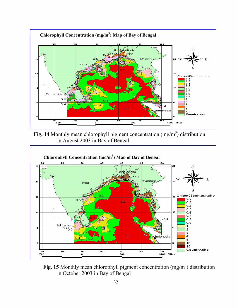
Fig. 14 Monthly mean chlorophyll pigment concentration (mg/m3) distribution in August 2003 in Bay of Bengal
Chlorophyll Concentration (mg/m3) Map of Bay of Bengal
Chlorophyll Concentration (mg/m3) Map of Bay of Bengal
Fig. 15 Monthly mean chlorophyll pigment concentration (mg/m3) distribution in October 2003 in Bay of Bengal
32

Table 5 Basin averaged chlorophyll pigment concentrations (mg/m3) with its
maximum and Minimum value during different months in the year 2003
Chlorophyll Concentration (mg/m3)Month of
2003Minimum Maximum Average
January 0.06 10 0.3
April 0.025 10 0.28
July 0.05 10 0.4
August 0.03 10 0.4
October 0.04 10 0.44
33

Seasonal cycle of sea surface height anomalies
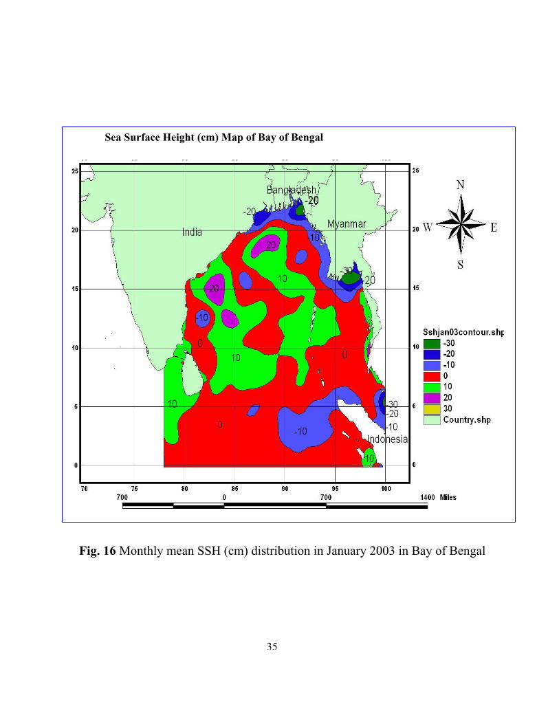
The sea surface height (SSH) anomaly distribution in January showed alternate band of
negative and positive anomaly along the eastern boundary form south to north (Fig.16). In the
rest of the region the SSH anomaly is positive except near the eastern equatorial region and a
few isolated pockets. In April, along the western boundary we notice series of positive and
negative SSH anomalies embedded in a region of positive anomaly (Fig.17). These could be
the regions of warm (positive SSH) and cold (negative SSH) core eddies. In July alternative
bands of positive and negative SSH anomalies were noticed all along the eastern and western
boundary (Fig.18). Open Bay of Bengal, in general, had positive SSH anomaly. The negative
SSH anomaly seen off Godavari river in April becomes much more negative by July. In
August, high SSH anomaly is seen along the eastern boundary right from equator expending
up to the northern part of the western boundary (Fig.19). In fact, positive SSH anomaly
occupies the entire bay, except a few regions including Indo-Sri Lanka. The negative SSH
anomaly seen off the Godavari river now gets detached and appeared to have move further
offshore. In October pattern of SSH anomaly was similar to that of August, but magnitude of
the anomaly was smaller in the open Bay (Fig.20). All along the coastal boundary SSH
anomaly remained positive. Off Irrawady and Ganges the positive SSH anomaly, 50-60 cm,
was the highest.
34
Sea Surface Height (cm) Map of Bay of Bengal
Fig. 16 Monthly mean SSH (cm) distribution in January 2003 in Bay of Bengal
35

Sea Surface Height (cm) Map of Bay of Bengal
Fig. 17. Monthly mean SSH (cm) distribution in April 2003 in Bay of Bengal
Sea Surface Height (cm) Map of Bay of Bengal
Fig. 18. Monthly mean SSH (cm) distribution in July 2003 in Bay of Bengal
36

Fig. 19. Monthly mean SSH (cm) distribution in August 2003 in Bay of Bengal
Fig. 20. Monthly mean SSH (cm) distribution in October 2003 in Bay of Bengal
37

Seasonal cycle of sea surface wind
For the analysis of variability of sea surface winds the U-component of the wind (zonal
wind, East-West) and V-component of the wind (meridional wind, North-South) were
analyzed.
The sea surface wind (SSW) was northeasterly in January in the entire Bay with maximum
velocity in the central region. In April the SSW was northeasterly in the eastern Bay while
it was southwesterly towards the western boundary with small magnitude (Fig.21a and
21b). In fact his showed that the Bay experiences light and variable winds during this time
of the year. By July the entire Bay is under the influence of strong southwesterly monsoon
winds with maximum speed of about 10-11m/s. In August also the SSW pattern was
similar to that of July with wind speed of 10m/s. However, near the southeastern and
southwestern parts the wind speed was less (Fig.22a and 22b). In October the southwesterly
wind with stronger zonal component was confined to the southern Bay and the wind speed
showed a gradual decrease towards north. In the north the westerly component is replace by
easterly component.
38
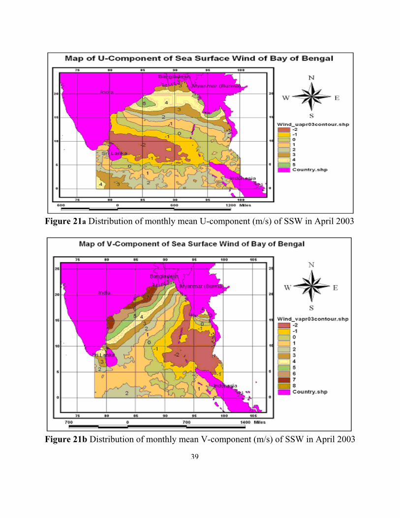
Figure 21a Distribution of monthly mean U-component (m/s) of SSW in April 2003
Figure 21b Distribution of monthly mean V-component (m/s) of SSW in April 2003
39

Fig. 22a Distribution of monthly mean U-component (m/s) of SSW in August 2003
Fig 22b Distribution of monthly mean V-component (m/s) of SSW in August 2003
40

Inter-annual variability during 2002-2005
To understand the inter-annual variability we selected the month of January and August during
2002 to 2005. The reason for selecting January and August is the following. The month of
January represents the peak winter, which is reflected in the property distribution such as SST,
SSW, SSH, and chlorophyll pigment concentrations. Similarly, the analysis of seasonal
variability showed that Chlorophyll concentration, SST and SSH showed maximum variability
in the month of August, while SSW was strongest in July. Since the wind being the forcing for
oceanic variability, and there exists time lag between the forcing and response, we thought it
may be a good idea to choose the month of August to track inter-annual variability in
chlorophyll concentration, SST and SSH while July for SSW.
Inter-annual variability of Sea surface temperature
January 2002 - 2005
The distribution of SST during January 2002 showed very cold temperature in the northern
Bay of Bengal, as low as 17oC while the southern Bay was warm with temperature 29oC
(Figure 23). The northern Bay, north of 15oN showed large thermal gradient, about 9oC, while
that in the southern bay was only about 3oC. In January 2003 the northern Bay was much less
colder compared to 2002 with the lowest temperature of 21oC. In the south, Bay was about 2oC
warmer in 2003 compared to 2002 (Figure 24). Thus, in general, January 2002 was colder
much colder than 2003. SST magnitude and distribution pattern of January 2004 was similar to
that of 2003 (Figure 25). SST in January 2005 was slightly colder than that of 2004 in the
southern Bay (Figure 26).
41

Fig.23 Monthly mean SST (oC) distribution in Bay of Bengal in January 2002
Distribution of Sea Surface Temperature (oC) in Bay of Bengal
Distribution of Sea Surface Temperature (oC) in Bay of Bengal
Fig.24 Monthly mean SST (oC) distribution in Bay of Bengal in January 2003
42

Fig.25 Monthly mean SST (oC) distribution in Bay of Bengal in January 2004
Distribution of Sea Surface Temperature (oC) of Bay of Bengal
Distribution of Sea Surface Temperature (oC) in Bay of Bengal
Fig.26 Monthly mean SST (oC) distribution in Bay of Bengal in January 2005
43
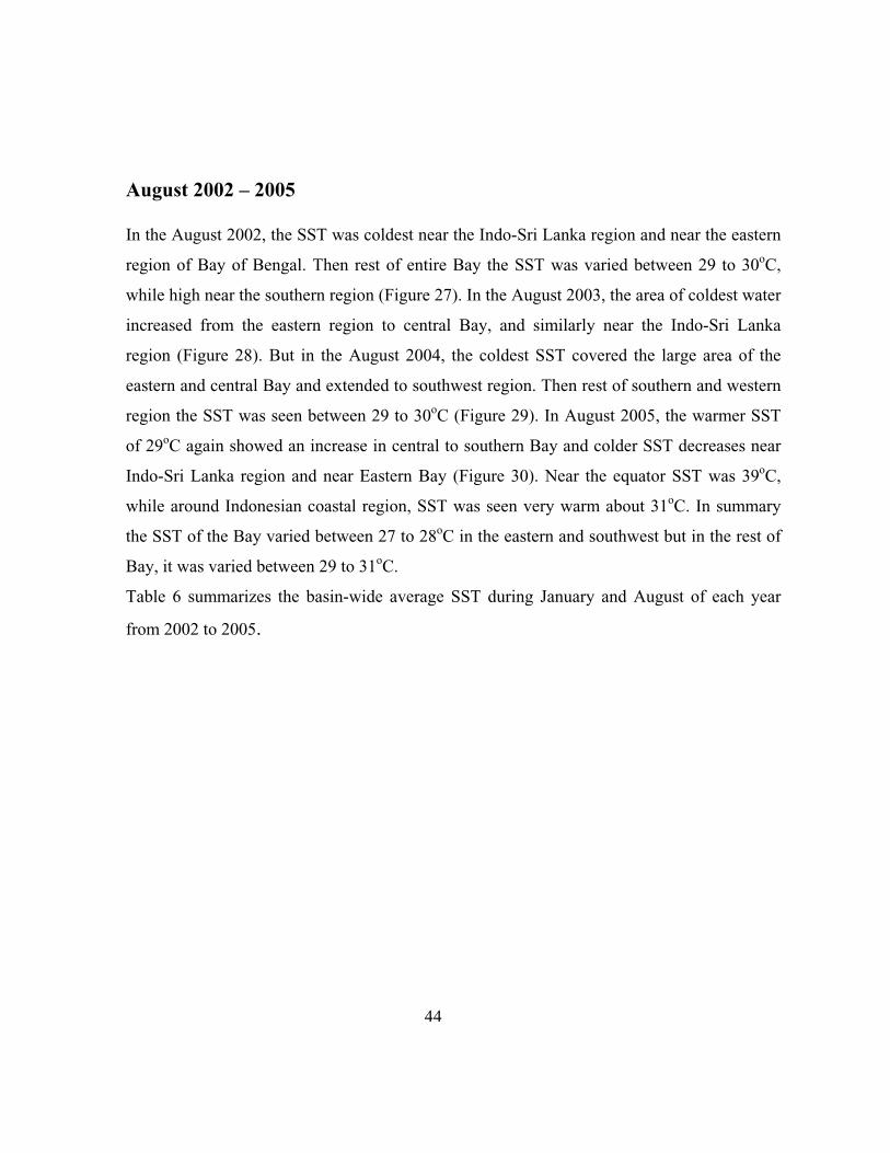
August 2002 – 2005
In the August 2002, the SST was coldest near the Indo-Sri Lanka region and near the eastern
region of Bay of Bengal. Then rest of entire Bay the SST was varied between 29 to 30oC,
while high near the southern region (Figure 27). In the August 2003, the area of coldest water
increased from the eastern region to central Bay, and similarly near the Indo-Sri Lanka
region (Figure 28). But in the August 2004, the coldest SST covered the large area of the
eastern and central Bay and extended to southwest region. Then rest of southern and western
region the SST was seen between 29 to 30oC (Figure 29). In August 2005, the warmer SST
of 29oC again showed an increase in central to southern Bay and colder SST decreases near
Indo-Sri Lanka region and near Eastern Bay (Figure 30). Near the equator SST was 39oC,
while around Indonesian coastal region, SST was seen very warm about 31oC. In summary
the SST of the Bay varied between 27 to 28oC in the eastern and southwest but in the rest of
Bay, it was varied between 29 to 31oC.
Table 6 summarizes the basin-wide average SST during January and August of each year
from 2002 to 2005.
44

Fig.27 Monthly mean SST (oC) distribution in Bay of Bengal in August 2002
Distribution of Sea Surface Temperature (oC) in Bay of Bengal
Distribution of Sea Surface Temperature (oC) in Bay of Bengal
Fig.28 Monthly mean SST (oC) distribution in Bay of Bengal in August 2003
45

Fig.29 Monthly mean SST (oC) distribution in Bay of Bengal in August 2004
Distribution of Sea Surface Temperature (oC) in Bay of Bengal
Distribution of Sea Surface Temperature (oC) in Bay of Bengal
Fig.30 Monthly mean SST (oC) distribution in Bay of Bengal in August 2005
46

Table 6 summarizes the basin-wide average SST (oC) during January and
August of each year from 2002 to 2005.
Sea Surface Temperature (oC) in January 2002-2005
Sea Surface Temperature (oC) in August 2002-2005 Year
Minimum Maximum Average Minimum Maximum Average
2002 15 30 29 26 31 29
2003 21 31 28 26 31 28
2004 22 31 28 26 31 28
2005 22 31 29 26 31 29
47

Inter-annual variability of chlorophyll concentration
January 2002-2005
During winter monsoon in the month of January 2002, the chlorophyll concentrations
varied between 0.2 to 0.4 mg/m3 in most part of the Bay except very near to the coast. In
fact large part of the Bay had a pigment concentration of about 0.3 mg/m3. In the central
Bay as well as near the equatorial belt the concentrations were about 0.2 mg/m3. All along
the coastal boundary the concentrations increased rapidly from 0.4 to 10 mg/m3. Maximum
pigment concentrations were noticed near the coastal area of Bangladesh and Irrawadi river
basin in the eastern Bay where the rivers discharge the fresh water. But these values needs
to be interpreted with care as near the coast there may be large amount of suspended
sediment which may introduce some errors in the pigment concentration estimation (Figure
31). In January 2003, the distribution pattern remains more or less same, but the
concentrations in most part of the Bay were about 0.2 mg/m3, which is less than that of
January 2002 (Figure 32). Again, in January 2004 the area of both 0.2 and 0.3 mg/m3
chlorophyll pigment concentrations showed an increase, but were much less than that of
2002 (Figure 33). Similarly in January 2005 the area of 0.2mg/m3 chlorophyll pigment
concentration showed an increase, which is much more than 2004 while the area of
0.3mg/m3 chlorophyll concentrations showed a decrease. In western Bay, near the
Mahanadi river basin, chlorophyll showed the poor concentration comparison to 2004
(Figure 34).
In summary, the chlorophyll concentration showed the high values between 5 to 10 mg/m3
mainly near the coastal areas of northern and eastern region due to upwelling and high
sedimentation due to fresh water and showed the low value in the open Bay and southern
region due to high solar heating.
48

Fig. 31 Monthly mean Chlorophyll Pigment Concentration (mg/m3) distribution in Bay of Bengal in January 2002
Chlorophyll Concentration (mg/m3) Map of Bay of Bengal
Chlorophyll Concentration (mg/m3) Map of Bay of Bengal
Fig. 32 Monthly mean Chlorophyll Pigment Concentration (mg/m3) distribution in Bay of Bengal in January 2003
49

Fig. 33 Monthly mean Chlorophyll Pigment Concentration (mg/m3) distribution in Bay of Bengal in January 2004
Chlorophyll Concentration (mg/m3) Map of Bay of Bengal
Chlorophyll Concentration (mg/m3) Map of Bay of Bengal
Fig. 34 Monthly mean Chlorophyll Pigment Concentration (mg/m3) distribution in Bay of Bengal in January 2005
50

August 2002 to 2005
In the august 2002, the chlorophyll concentrations were seen high near the coastal areas of
Ganges-Brahmputra-Meghna deltaic and Irrawadi region. Then in the other coastal areas it
varied between 0.4 to 5 mg/m3. But one patch of chlorophyll concentration greater than 0.5
mg/m3 was seen near the Indo-Sri Lanka region, which extends to central Bay. In the most
part of central Bay, the chlorophyll concentration was about 0.3mg/m3 but in the southern
region it was seen 0.2mg/m3 (Figure 35). In the August 2003, the chlorophyll concentration
showed the low values near the coastal areas compared to August 2002. Near the Irrawady
River basin it showed low concentration about 0.3mg/m3 and similar near the Indo-Sri
Lanka region the area of high concentration showed a decrease. Most of the central and
southern Bay, concentrations was about 0.2mg/m3 (Figure 36). But in August 2004, again it
showed the high concentration near the coastal areas. The chlorophyll concentration was
very high with the values of 0.4 to 2 mg/m3 near the Indo-Sri Lanka region which extend in
the northeastward direction into the central Bay. The chlorophyll concentration was low in
the southern Bay and most of central Bay, with concentration of about 0.3mg/m3 (Figure
37). In August 2005, the chlorophyll distribution pattern was similar to that of August 2004
near the coastal areas and near the Indo-Sri Lanka region, but the area of 0.2mg/m3
concentration showed an increase near the Krishna and Godavari region and in central Bay
(Figure 38). Table 7 shows basin averaged chlorophyll pigment concentrations with its
maximum and minimum value during January and August of each year from 2002 to 2005.
51

Chlorophyll Concentration (mg/m3) Map of Bay of Bengal
Fig. 35 Monthly mean Chlorophyll Pigment Concentration (mg/m3) distribution in Bay of Bengal in August 2002
Chlorophyll Concentration (mg/m3) Map of Bay of Bengal
Fig. 36 Monthly mean Chlorophyll Pigment Concentration (mg/m3) distribution in Bay of Bengal in August 2003
52

Fig. 37 Monthly mean Chlorophyll Pigment Concentration (mg/m3) distributionIn Bay of Bengal in August 2004
Chlorophyll Concentration (mg/m3) Map of Bay of Bengal
Chlorophyll Concentration (mg/m3) Map of Bay of Bengal
Fig. 38 Monthly mean Chlorophyll Pigment Concentration (mg/m3) distributionIn Bay of Bengal in August 2005
53

Table 7 Basin averaged chlorophyll pigment concentrations with its maximum
and minimum value during January and August of each year from 2002 to 2005.
Chlorophyll Concentration (mg/m3) in January 2002-2005
Chlorophyll Concentration (mg/m3) in August 2002-2005
YearMinimum Maximum
AverageMinimum Maximum Average
2002 0.05 15 0.4 0.05 15 0.4
2003 0.06 10 0.4 0.03 10 0.4
2004 0.06 10 0.4 0.06 15 0.4
2005 0.05 10 0.4 0.04 10 0.4
54
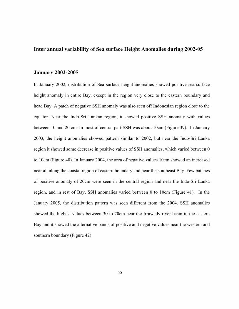
Inter annual variability of Sea surface Height Anomalies during 2002-05
January 2002-2005
In January 2002, distribution of Sea surface height anomalies showed positive sea surface
height anomaly in entire Bay, except in the region very close to the eastern boundary and
head Bay. A patch of negative SSH anomaly was also seen off Indonesian region close to the
equator. Near the Indo-Sri Lankan region, it showed positive SSH anomaly with values
between 10 and 20 cm. In most of central part SSH was about 10cm (Figure 39). In January
2003, the height anomalies showed pattern similar to 2002, but near the Indo-Sri Lanka
region it showed some decrease in positive values of SSH anomalies, which varied between 0
to 10cm (Figure 40). In January 2004, the area of negative values 10cm showed an increased
near all along the coastal region of eastern boundary and near the southeast Bay. Few patches
of positive anomaly of 20cm were seen in the central region and near the Indo-Sri Lanka
region, and in rest of Bay, SSH anomalies varied between 0 to 10cm (Figure 41). In the
January 2005, the distribution pattern was seen different from the 2004. SSH anomalies
showed the highest values between 30 to 70cm near the Irrawady river basin in the eastern
Bay and it showed the alternative bands of positive and negative values near the western and
southern boundary (Figure 42).
55

Figure 39 Monthly mean SSH (cm) distribution in Bay of Bengal in January 2002
Figure 40Monthly mean SSH (cm) distribution in Bay of Bengal in January 2003
56

Figure 41 Monthly mean SSH (cm) distribution in Bay of Bengal in January 2004
Figure 42 Monthly mean SSH (cm) distribution in Bay of Bengal in January 2005
57

August 2002-2005
In August 2002, the sea surface height anomaly showed high positive values near the eastern
and northern boundary of the Bay, and extending to equator towards eastern boundary
(Figure 43). But in the western region, near the Godavari and Krishna region negative
pockets of SSH anomaly of –10 cm and same as around Sri Lanka region except one patch
of –20cm. In the August 2003, the SSH anomaly showed the similar distribution pattern to
August 2002, except negative patch of –10 to –20cm in near the Mahanadi river basin
(Figure 44). In the August 2004, the negative patches of –10 cm increased in the open Bay
towards the western Bay (Figure 45). In the August 2005, the negative SSH anomalies were
seen in the eastern and towards the western open region. Then in the rest of part SSH
anomaly showed the positive values (Figure 46). In general, negative SSH anomaly was seen
near along the western boundary while it was positive in the rest of the Bay of Bengal. In
particular the highest positive SSH was noticed along the eastern Bay.
58

Figure 43 Monthly mean SSH (cm) distribution in Bay of Bengal in August 2002
Figure 44 Monthly mean SSH (cm) distribution in Bay of Bengal in August 2003
59

Figure 45 Monthly mean SSH (cm) distribution in Bay of Bengal in August 2004
Figure 46 Monthly mean SSH (cm) distribution in Bay of Bengal in August 2005
60


CHAPTER 5
Summary and Conclusion
Summary
The Bay of Bengal is a northern extended arm of the Indian Ocean, situated in eastern part
between equator and 220N latitude and 800E and 1000E longitude. It is a tropical basin,
landlocked in the north by the landmasses of India and Bangladesh and the deltaic region of
the Ganges-Brahmaputra-Meghna river system, in the east by the Myanmar peninsula and
Indonesian archipelago, and in the west by peninsular India and east coasts of Sri Lanka. The
southern boundary of the Bay is in contact with southern ocean. The winds over the Bay of
Bengal (BoB) undergo seasonal changes from north-easterly (November-February) during
winter to south-westerly (June-September) during summer monsoon. In response to these
winds, the environmental/oceanographic characteristics of the Bay of Bengal also will
undergo seasonal changes. In addition, the large amount of refresh water brought by the
rivers such as Ganges, Brahmaputra, Irawady, Mahanadi, Krishna, Godavari and Kaveri
adjoining the BoB also will play a major role in the hydrographic characteristics. Hence the
present study aims at understanding the seasonal variability of the environmental parameters
of B ay of Bengal.
The present study utilizes the tools such as Geographical Information System (GIS) and
remote sensing for the analysis of environment parameters of Bay of Bengal. The remote
sensing data, used in the study, are Sea Surface Temperature (SST), Sea Surface Height
(SSH) anomalies, Chlorophyll Concentration and Sea Surface Wind. The monthly mean data
on SST is from Modis Aqua, chlorophyll pigment concentrations is from SeaWiFS, and sea
surface winds from Quikscat. Monthly mean sea surface height anomalies were obtained
merged 7-day snap shot from Topex/Posidon and ERS-1/2 series of satellites. The spatial
resolution of all the data is 0.3degree in latitude and longitude. The data used for the present
study is from January 2002 to December 2005.
61

These data were analyzed using GIS to determine the seasonal and inter-annual variability.
GIS facilitates the modeling and analysis of data apart from generation of contours maps and
database of these maps.
The seasonal cycle of SST in the Bay of Bengal showed two periods of warming during April
and October. In this season SST was seen very warm with 29 to 30oC average in entire Bay,
while it showed the cooling during winter monsoon in month of January due to reduced solar
heating and upwelling near the coastal areas. The average SST was seen around 28oC with
minimum 22oC in northern coastal region. In summer monsoon, SST was also seen warm
with 29oC in entire Bay, while showed cooling near the eastern Bay due to upwelling of cold
water with 27oC to 28oC.
Seasonal cycle of chlorophyll concentration was high during summer monsoon, in the month
of July and August, and just after that in month of October and little more in January
(winter). Mostly chlorophyll pigment showed the high concentration near the coastal region
of the Bay and especially near the river mouths with high values about 5 to 10mg/m3. This
may be to large quantity of sediments discharged from major rivers, which also brings along
with them substantial quantities of nutrients, which supports the observed high pigment
concentration. The average chlorophyll concentration of 0.4mg/m3 was found in open Bay,
while in month of January and April; it showed low concentration in comparison to summer
monsoon in the open Bay as well as near the coastal areas. As a result most of coastal areas
of Bay of Bengal becomes biologically productive but in the open and southern Bay, the
productivity may becomes very low due to high SST in the open Bay and southern Bay of
Bengal.
Seasonal cycle of sea surface height in the Bay of Bengal showed the positive values mostly
in entire Bay except near the coastal areas of Northern and eastern Bay and few patches near
the western boundary. Large variation in positive and negative pockets of SSH was seen near
the western and eastern boundary in all months, these could be the regions of warm (positive
SSH) and cold (negative SSH) core eddies.
62

Seasonal cycle of sea surface wind showed the light and variable northeasterly wind in the
month of January (winter) and April (spring inter monsoon) but in the summer monsoon, it
was southwesterly with high speed about 10 to 11m/s. After summer monsoon, in fall inter
monsoon, it showed the little decreased in speed.
The analysis of seasonal cycle showed the positive relationship between chlorophyll
concentration and SST near the coastal areas of the Bay of Bengal, especially near the
northern and eastern Bay in the winter monsoon and it showed the inverse relationship in the
central and southern Bay of Bengal, during all the seasons, that means high SST, low
chlorophyll concentrations.
The analysis of SST, chlorophyll pigment concentration, sea surface height during 2002 to
2005 showed large inter-annual variability during both winter (January) and summer
(August). In general, high chlorophyll concentrations occurred during colder winter and
strong summer monsoon years while the SST was colder in the winter and very warmer in
the summer monsoon.
Conclusion
The study showed that the distribution of chlorophyll concentration was high near the coastal
region and it showed positive relationship to sea surface temperature during winter monsoon
near the northern coastal region but in the open Bay and southern Bay, inverse relationship
was seen between chlorophyll concentration and SST in all the months.
The high chlorophyll concentration was seen in the summer monsoon and also in fall inter
monsoon, near the coastal areas and Indo-Sri Lanka region. These regions could be the
highly biologically productive in the Bay of Bengal.
These results showed the Bay of Bengal low productive in the open and southern region, but
it is high biologically productive near shore region of all coastal boundaries (northern,
western and eastern Bay), especially near the river mouths.
63

References
Varkey, M.J., V.S.N. Murthy and A Suryanarayana (1996) Physical oceanography of Bay of
Bengal and Andaman sea, Oceanography and Marine biology: An annual review, 34, 1-70.
Prasanna Kumar, S. and A.S. Unnikrishnan (1995) Seasonal cycle of temperature and associated
wave phenomena in the upper layers of the Bay of Bengal, J. Geophys. Res., 100, 13585-13593.
Caloz, R. and C. Collet. 1997. GIS and remote sensing in the aquatic botany:
Kirk, J.T.O. 1994. Light and Photosynthesis in Aquatic Ecosystems, Cambridge University
Press, Cambridge;
Lehmann, A. and J. B. Lachavanne. 1997. GIS and remote sensing in aquatic botany.
McCreary, J.P., P. K. Kundu and R. L. Molinari, A numerical investigation of the dynamics and
mixed layer processes in the Indian Ocean, Prog. Oceanogr., 31, 181-244,1993.
Simpson, J.J. 1992. Remote sensing and GIS: their past, present and future use in global marine
fisheries.
Fu, L.-L., et al., TOPEX/POSEIDON Mission Overview, J. Geophys. Res., 99, 24,369-24,381,
1994.
Mitchum, G., Comparison of TOPEX sea surface heights and tide gauge sea levels.
64


