
Ballistic Limit Velocity For Continuous Fiber Polymeric
Composite Materials and Polymers Through Experimental and
Numerical Methods
by
Jonathan Scott Grupp
A thesis submitted to the Graduate Faculty of Auburn University
in partial fulfillment of the requirements for the Degree of
Doctorate of Philosophy
Auburn, Alabama May 10, 2015
Keywords: ballistic impact, LS-DYNA, composites, viscoplastic, finite element
Copyright 2015 by Jonathan Scott Grupp
Approved by
David Beale, Chair, Professor of Mechanical Engineering Royall Broughton, Professor Emeritus of Polymer Fiber Engineering Pradeep Lall, Thomas Walter Professor of Mechanical Engineering
Jeffrey Suhling, Department Head of Mechanical Engineering

Abstract
Composite materials are often subject to harsh operating environments which may include
impact from errant projectiles of various geometries traveling at specific velocities and trajectories.
Experimentalists seek to establish the ballistic limit velocity of the composite material where the
composite absorbs all of the energy of the projectile traveling at an initial velocity. An analytical
approach for the impact event can be difficult to reliably establish the ballistic limit of a particular
composite material due to the nonlinear response including rate dependency and post-failure behavior.
The finite element method has shown to be capable of modeling the impact event. However many
available material models require calibration from the experimental impact tests.
The goal of the present research is to develop and implement an efficient finite element
simulation of the composite material under impact which does not require calibration. A general
orthotropic viscoplastic material model will be presented. The viscoplastic model utilizes a more
generalized form of plastic potential than previous works in that it allows plasticity to occur in the fiber
direction. The model represents the nonlinear post-failure behavior through the Continuum Damage
Mechanics framework by utilizing an energy balance approach. Additionally a smeared crack model
algorithm is utilized to reduce the mesh dependency inherent to finite element solutions. The material
model was implemented for the explicit integration solver in LS-DYNA. An implicit return mapping
algorithm was utilized to integrate the material model response for each load step. The material model
was validated using data from published impact testing and material characterization. The finite element
simulations show that the material model is able to predict the ballistic limit velocity within a reasonable
margin.
ii

Impact experiments were performed using a single-stage light gas gun. The response of standard
aerospace-grade satin weave T300 carbon fiber panels using thermoplastic and thermoset matrices
were compared. The ballistic limit velocities for the aforementioned composites were determined using
a high speed video camera.
Ballistic testing was also performed on polycarbonate panels towards the development of
standardized test methods for ‘chainshot’ hazards present in the operation of the timber harvesting
operations. The experimental impact results were also simulated using finite element analysis. The
numerical results were compared to the experiment.
iii

Table of Contents
Abstract ......................................................................................................................................................... ii
List of Figures .............................................................................................................................................. vii
Chapter 1 : Introduction ............................................................................................................................... 1
1.1 : Research Outline ............................................................................................................................... 4
Chapter 2 : Experimental Setup .................................................................................................................... 6
2.1 : Gas Gun Design ................................................................................................................................. 6
2.2 : Barrel Design ..................................................................................................................................... 8
2.3 : Sabot Design ..................................................................................................................................... 9
2.4 : Gas Gun Implementation ................................................................................................................ 10
2.5 : Gas Gun Design Performance ......................................................................................................... 19
2.6 : Sabot Design Implementation ........................................................................................................ 22
2.7 : Sabot Design Validation .................................................................................................................. 27
Chapter 3 : Velocity Measurement ............................................................................................................. 30
3.1 : High Speed Camera ......................................................................................................................... 30
3.2 : Velocity Calculations Using Image Processing ................................................................................ 32
Chapter 4 : Composite Panel Ballistic Impact Testing Results .................................................................... 40
4.1 : Introduction .................................................................................................................................... 40
4.2 : Ballistic Impact Comparison of Thermoplastic and Epoxy Based Composites ............................... 42
4.3 : Falling Object Hazard, Ballistic Impact With Large Diameter Projectiles........................................ 48
Chapter 5 : Viscoplastic Composite Model ................................................................................................. 55
5.1 : Development of Sun’s Plastic Potential .......................................................................................... 55
5.2 : Derivation of Viscoplastic Model .................................................................................................... 58
5.3 : Return Mapping Algorithm ............................................................................................................. 64
5.4 : Material Parameter Determination Procedure .............................................................................. 69
iv

5.5 : Material Parameter Determination Algorithm ............................................................................... 72
5.6 : IM7/8552 Parameter Determination .............................................................................................. 75
Chapter 6 : Coupled Viscoplastic Progressive Damage Model ................................................................... 83
6.1 : Continuum Damage Mechanics Approach ..................................................................................... 83
6.2 : Viscoplastic Model Within Damage Mechanics Framework ........................................................... 84
6.3 : Energy-Based Damage Progression ................................................................................................ 86
6.4 : Smeared Crack Model ..................................................................................................................... 91
6.5 : Erosion Algorithm ........................................................................................................................... 95
6.6 : Material Model Assumptions And Limitations ............................................................................... 97
6.7 : LS-DYNA Implementation ............................................................................................................... 99
6.7.1 : LS-DYNA UMAT Overview ...................................................................................................... 100
6.7.2 : Smeared Crack Model Algorithm ........................................................................................... 101
6.7.3 : Viscoplastic Return Mapping Algorithm ................................................................................ 103
6.7.4 : Damage Model Algorithm ...................................................................................................... 108
6.7.5 : Erosion Criteria Algorithm ...................................................................................................... 110
6.8 : LS-DYNA UMAT Model Validation ................................................................................................. 111
6.8.1 : IM7/8552 Material Model Parameters .................................................................................. 112
6.8.2 : LS-DYNA User Defined Material Implementation Validation ................................................ 116
6.8.3 : Off-Axis Loading With Damage Behavior ............................................................................... 123
6.8.4 : Cyclic Loading ......................................................................................................................... 126
6.8.5 : Mesh Sensitivity Study ........................................................................................................... 126
Chapter 7 : IM7/8552 Ballistic Impact Simulation Results ........................................................................ 132
7.1 : Backplane Deflection .................................................................................................................... 136
7.2 : Damage Progression ..................................................................................................................... 138
7.3 : Ballistic Limit Velocity ................................................................................................................... 139
Chapter 8 : Polycarbonate Glazing Experimental Test Methodology ....................................................... 142
8.1 : Chainshot or Thrown Object Hazard ............................................................................................. 142
8.2 : Chainshot Fragment Simulating Projectile ................................................................................... 146
8.3 : Test Setup ..................................................................................................................................... 148
8.4 : Experimental Test Results ............................................................................................................. 152
8.4.1 : 0.5” Monolithic Lexan Impact ................................................................................................ 152
v

8.4.2 : 0.75” Laminated Lexan Impact .............................................................................................. 156
Chapter 9 : Polycarbonate Glazing Ballistic Impact Simulations ............................................................... 160
9.1 : Polycarbonate Material Behavior ................................................................................................. 160
9.2 : LS-DYNA Polycarbonate Ballistic Impact Model............................................................................ 163
9.2.1 : Chain Fragment Steel Material Model ................................................................................... 165
9.2.2 : Polycarbonate Material Model .............................................................................................. 167
9.3 : LS-DYNA Simulation Results .......................................................................................................... 170
Chapter 10 : Conclusions .......................................................................................................................... 174
References ................................................................................................................................................ 178
vi

List of Figures
Figure 2.1: Push And Pull Sabots (Stilp et al, 1990) .................................................................................... 10 Figure 2.2: Experimental Gas Gun .............................................................................................................. 11 Figure 2.3: Experimental Safety Enclosures ................................................................................................ 11 Figure 2.4: Lamé Equation Definitions; Thick-walled Cylinder Under Pressure ......................................... 13 Figure 2.5: Experimental Gas Gun Support System Upgrade ..................................................................... 15 Figure 2.6: Barrel Center Support With Linear Bearing .............................................................................. 16 Figure 2.7: Barrel End Support .................................................................................................................... 16 Figure 2.8: CAD Gas Gun Model Recoil Simulation ..................................................................................... 17 Figure 2.9: Experimental Gas Gun Upsized Barrel Configuration ............................................................... 18 Figure 2.10: Upsized Barrel Delrin Bushing; Center Support ...................................................................... 18 Figure 2.11: Upsized Barrel Delrin Bushing; End Support ........................................................................... 19 Figure 2.12: Projectile Velocity As A Function Of Pressure For Air ............................................................. 20 Figure 2.13: Projectile Velocity As A Function Of Pressure For Helium ...................................................... 21 Figure 2.14: Projectile Impact Location ...................................................................................................... 22 Figure 2.15: CAD Representation of Sabot Design With Spherical Projectile ............................................. 23 Figure 2.16: Completed Sabot With Spherical Projectile ............................................................................ 24 Figure 2.17: Assembled Sabot ..................................................................................................................... 25 Figure 2.18: Prototype Shear Jig ................................................................................................................. 25 Figure 2.19: Prototype Shear Jig Mounted In Drill Press ............................................................................ 26 Figure 2.20: Sample Of Sabots Manufactured ............................................................................................ 26 Figure 2.21: Projectile Trajectory Deviations, Attitude (Zukas, 1990) ........................................................ 27 Figure 2.22: High Speed Video Stills Of Sabot Design Validation................................................................ 28 Figure 2.23: Sabot Stripper Plates ............................................................................................................... 29 Figure 3.1: High Speed Video Camera Used For Velocity Measurements .................................................. 31 Figure 3.2: High Speed Video Frames From Composite Panel Ballistic Impact .......................................... 32 Figure 3.3: Metric Board During Calibration Of High Speed Video Camera ............................................... 33 Figure 3.4: Velocity Calculation Program GUI ............................................................................................. 33 Figure 3.5: Video Data Trimmed And Cropped ........................................................................................... 35 Figure 3.6: Pixel Intensity Adjusted ............................................................................................................ 36 Figure 3.7: Image Inversion ......................................................................................................................... 36 Figure 3.8: Centroid Data Calculated For Video Frame Images .................................................................. 37 Figure 3.9: X- And Y-Velocity Plot Output ................................................................................................... 37 Figure 3.10: Unprocessed Baseball Impact Video ....................................................................................... 38 Figure 3.11: Processed Baseball Impact Video ........................................................................................... 38 Figure 3.12: COR Output Results ................................................................................................................ 39
vii

Figure 3.13: COR Algorithm; Determination of Minimum Acceleration ..................................................... 39 Figure 4.1: V50 And The Zone Of Mixed Results (Solsby, 1987) ................................................................. 41 Figure 4.2: CAD Representation Of Test Sample Fixture (AMRDEC, 2010)................................................. 44 Figure 4.3: 1/4" Diameter Spherical Projectile With Sabot ........................................................................ 45 Figure 4.4: 0° Obliquity Ballistic Performance Thermoplastic And Epoxy Comparison .............................. 48 Figure 4.5: 45° Obliquity Ballistic Performance Thermoplastic And Epoxy Comparison ............................ 48 Figure 4.6: 1-3/8" Spherical Sabot .............................................................................................................. 49 Figure 4.7: Assembled 1-3/8" Spherical Sabot With Projectile................................................................... 50 Figure 4.8: CAD Representation Of Large Projectile Test Fixture (AMRDEC, 2012) ................................... 50 Figure 4.9: High Speed Video Stills Of Large Projectile Sabot Development; 658 fps ................................ 51 Figure 4.10: COR As Function Of Sample Thickness .................................................................................... 53 Figure 4.11: Test Fixture Mid-span Deflection ............................................................................................ 54 Figure 5.1: Stress-strain curves of Kevlar 49 fiber bundles, Wang et al (34) .............................................. 57 Figure 5.2: 3-D General Return Mapping Algorithm ................................................................................... 66 Figure 5.3: 1-D Uniaxial Off-Axis Return Mapping Algorithm ..................................................................... 73 Figure 5.4: IM7/8552 15° Off-Axis .............................................................................................................. 76 Figure 5.5: IM7/8552 30° Off-Axis .............................................................................................................. 77 Figure 5.6: IM7/8552 60° Off-Axis .............................................................................................................. 77 Figure 5.7: Master Curve Effective Stress vs. Effective Plastic Strain for IM7/8552 ................................... 78 Figure 5.8: Log-Log Transformation of Master Curve IM7/8552 Data ....................................................... 79 Figure 5.9: IM7/8552 Power Law Hardening Rule Fit ................................................................................. 79 Figure 5.10: Linear Regression Calculation for χ and m Parameters .......................................................... 80 Figure 5.11: IM7/8552 Stress vs Strain; Comparison of Model to Fitted Data; Static Cases ...................... 81 Figure 5.12: IM7/8552 Stress vs Strain; Comparison of Model to Fitted Data; Dynamic Cases ................. 81 Figure 5.13: IM7/8552 Stress vs Strain; Comparison of Model to Experimental Data; Static Cases .......... 82 Figure 5.14: IM7/8552 Stress vs Strain; Comparison of Model to Experimental Data; Dynamic Cases ..... 82 Figure 6.1: Energy Contributions to Total Fracture Energy ........................................................................ 88 Figure 6.2: Comparison of Energy Dissipation for Polynomial and Linear Damage Progression ............... 90 Figure 6.3: 1-D Uniaxial Tensile Damage Progression ................................................................................ 91 Figure 6.4: Isoparametric Coordinate System and Element Node Numbering for Hexahedral Element ... 93 Figure 6.5: Virtual Mid-planes of Hexahedral Element (a) in-plane failure modes (b) out-of-plane failure modes.......................................................................................................................................................... 93 Figure 6.6: Material Model Energy Dissipation Due To Elastic, Plastic, And Damage Contributions ......... 98 Figure 6.7: Coupled Viscoplastic Damage Material Model Flowchart ...................................................... 101 Figure 6.8: Smeared Crack Model Algorithm Flowchart ........................................................................... 103 Figure 6.9: Viscoplastic Return Mapping Algorithm ................................................................................. 105 Figure 6.10: Damage Model Algorithm Flowchart .................................................................................... 108 Figure 6.11: Normal Strain Damage Progression Algorithm ..................................................................... 109 Figure 6.12: Shear Strain Damage Progression Algorithm ........................................................................ 110 Figure 6.13: Erosion Criteria Algorithm .................................................................................................... 111 Figure 6.14: Populated LS-DYNA Keycard For Coupled Viscoplastic Damage UMAT ............................... 115 Figure 6.15: Off-Axis Tension Rotation About (a) Z-Axis (b) X-Axis........................................................... 117
viii

Figure 6.16: LS-DYNA Single Element Off-Axis Tension Boundary Conditions and Material Orientations for Rotations About: a) Z-Axis b) X-Axis ........................................................................................................ 118 Figure 6.17: LS-DYNA Comparison; Off-Axis Tension 0° Rotation About Z-Axis ....................................... 119 Figure 6.18: LS-DYNA Comparison; Off-Axis Tension 30° Rotation About Z-Axis ..................................... 119 Figure 6.19: LS-DYNA Comparison; Off-Axis Tension 60° Rotation About Z-Axis ..................................... 120 Figure 6.20: LS-DYNA Comparison; Off-Axis Tension 90° Rotation About Z-Axis ..................................... 120 Figure 6.21: LS-DYNA Comparison; Off-Axis Tension 0° Rotation About X-Axis ....................................... 121 Figure 6.22: LS-DYNA Comparison; Off-Axis Tension 30° Rotation About X-Axis ..................................... 122 Figure 6.23: LS-DYNA Comparison; Off-Axis Tension 60° Rotation About X-Axis ..................................... 122 Figure 6.24: LS-DYNA Comparison; Off-Axis Tension 90° Rotation About X-Axis ..................................... 123 Figure 6.25: 15° Off-Axis Compressive Loading With Damage Model; Strain Rate 122 1/sec ................. 124 Figure 6.26: 30° Off-Axis Compressive Loading With Damage Model; Strain Rate 246 1/sec ................. 125 Figure 6.27: 60° Off-Axis Compressive Loading With Damage Model; Strain Rate 367 1/sec ................. 125 Figure 6.28: Progressive Damage Of Uniaxial Tensile Cyclic Loading Case ............................................... 126 Figure 6.29: Mesh Sensitivity Coupon Boundary Conditions .................................................................... 127 Figure 6.30: Mesh Sensitivity Coupon Comparison .................................................................................. 127 Figure 6.31: Fracture Energy Dissipation Comparison .............................................................................. 128 Figure 6.32: Smeared Crack Model Mesh Convergence; Maximum Force vs Element Number .............. 129 Figure 6.33: Mesh Sensitivity Damage Study Coupon 1 ........................................................................... 129 Figure 6.34: Mesh Sensitivity Damage Study Coupon 2 ........................................................................... 130 Figure 6.35: Mesh Sensitivity Damage Study Coupon 3 ........................................................................... 130 Figure 6.36: Mesh Sensitivity Damage Study Coupon 4 ........................................................................... 131 Figure 6.37: Mesh Sensitivity Damage Study Coupon 5 ........................................................................... 131 Figure 7.1: LS-DYNA Ballistic Impact Simulation Model Boundary Conditions ......................................... 133 Figure 7.2: LS-DYNA Ballistic Model Composite Layup ............................................................................. 134 Figure 7.3: Mesh Convergence Study; Maximum Center Deflection at 54 mps Impact Velocity ............. 136 Figure 7.4: Moiré Fringe Experimental Data; 54 mps Impact Velocity ..................................................... 137 Figure 7.5: FEM Simulation Deflection Results; 54 mps Impact Velocity ................................................. 138 Figure 7.6: 𝒅𝒅𝒅𝒅𝒅𝒅 Damage Variable Ply Comparison; 54 mps Case ............................................................ 139 Figure 7.7: Comparison of Initial and Residual Velocities for IM7/8552 Ballistic Impact Simulations ..... 140 Figure 7.8: Element Distortion at 85 mps Impact Velocity; 140 μsec after impact .................................. 141 Figure 8.1: Plate Response To (a) Low And (b) High Velocity Impact ....................................................... 142 Figure 8.2: Chainshot Event Sequence (Oregon Mechanical Timber Harvesting Handbook, 2005) ........ 144 Figure 8.3: Experimental Chainshot Launcher (Skogforsk, 2004) ............................................................. 145 Figure 8.4: High Speed Video Stills of Chain Shot Event (Skogforsk, 2004) .............................................. 145 Figure 8.5: Harvester Chain Components (Oregon Mechanical Timber Harvesting Handbook, 2005) .... 147 Figure 8.6: Highest Potentially Hazardous Chainshot Fragments (Oregon, 2013) ................................... 147 Figure 8.7: CAD Representation Of Chainshot FSP ................................................................................... 148 Figure 8.8: Experimental Single-Stage Gas Gun System ........................................................................... 148 Figure 8.9: Trimmed Driving Link Chainshot FSP ...................................................................................... 149 Figure 8.10: CAD Representation Of General Sabot Design With Spherical Projectile............................. 150 Figure 8.11: Assembled Chainshot FSP Sabot ........................................................................................... 150
ix

Figure 8.12: Unassembled Chainshot FSP Sabot....................................................................................... 151 Figure 8.13: Sabot Design Validation High Speed Video Stills .................................................................. 152 Figure 8.14: 0.5" Monolithic Lexan Post-Impact Damage For Test 1; Isometric View ............................. 154 Figure 8.15: 0.5" Monolithic Lexan Post-Impact Damage For Test 4; Front Face..................................... 154 Figure 8.16: 0.5" Monolithic Lexan Post-Impact Damage For Test 4; Side View ...................................... 155 Figure 8.17: 0.5” Monolithic Lexan Impact – Test 5 High Speed Video Stills............................................ 156 Figure 8.18: 0.75" Laminated Lexan Post-Impact Damage For Test 1; Front Face ................................... 157 Figure 8.19: 0.75" Laminated Lexan Post-Impact Damage For Test 1; Front Close Up ............................ 158 Figure 8.20: 0.75" Laminated Lexan Post-Impact Damage For Test 3; Front Close Up ............................ 159 Figure 8.21: 0.75" Laminated Lexan Post-Impact Damage For Test 3; Back ............................................ 159 Figure 9.1: Polycarbonate Stress-Strain Relationship at Various Strain Rates (Moy et al) ....................... 160 Figure 9.2: Strength Differential of Polycarbonate (Boyce et al) .............................................................. 161 Figure 9.3: Polycarbonate Stress-Strain Relationship at Various Temperatures at 0.01 / second Strain Rate (Richeton et al) ................................................................................................................................. 162 Figure 9.4: Polycarbonate Yield Stress As Function of Strain Rate (Moy et al) ........................................ 162 Figure 9.5: Polycarbonate Yield Stress As Function of Strain Rate and Temperature (Richeton et al) .... 163 Figure 9.6: LS-DYNA FEM Model For Chainshot Impact ........................................................................... 164 Figure 9.7: Chain Fragment Assembly Finite Element Mesh .................................................................... 165 Figure 9.8: Steel Material Model Bilinear Response ................................................................................. 166 Figure 9.9: Polycarbonate Yield Stress As A Function of Strain Rate ........................................................ 169 Figure 9.10: Polycarbonate Tangent Modulus As A Function of Strain Rate ............................................ 169 Figure 9.11: 0.5" Monolithic Lexan Ballistic Impact Experimental Vs. FEM Comparison ......................... 171 Figure 9.12: Comparison Of Experimental And LS-DYNA Ballistic Event for Test 5 of Monolithic Testing .................................................................................................................................................................. 172 Figure 9.13: Progression of Effective Plastic Strain for Test 5 of Monolithic Testing ............................... 173
x

Chapter 1 : Introduction Composite materials are often utilized in harsh environments where the composite structure
can be subject to high velocity impact. It is therefore of the utmost importance for the designer to
understand the behavior of the composite structure resulting from the impact event. The composite
designer can use experimental testing, analytical models, and/or numerical methods to determine the
ballistic performance of the composite material. Experimental testing is the most reliable method to
determine the ballistic performance. However, experimental methods are expensive and time-
consuming. Analytical models typically rely on an energy balance and several factors or empirical
relationships to determine the ballistic performance. Although some analytical methods have shown to
be able to predict ballistic performance reasonably, very little additional insight regarding the impact of
the composite material can be garnered. Numerical methods such as the Finite Element Method (FEM)
can readily predict ballistic performance while also providing the analyst with additional insight to the
composite behavior due to the impact. However numerical methods require a significant understanding
of the composite behavior beforehand. This includes experimental material characterization test data
and a corresponding material model that can accurately represent the composite. As such, numerical
methods can be difficult to implement effectively. Given the aforementioned strengths and weaknesses
for each of the approaches, the pursuant research will utilize both experimental and numerical methods
to determine the ballistic performance of composites.
Composite materials are becoming more prevalent in a wider range of applications due to the
inherent advantages afforded by their strength to weight ratio over more traditional engineering
materials such as metals. However in recent years designers have placed an increased emphasis on
optimum structural performance. Through more advanced design tools and analysis, the optimum
composite design includes more focus on the specific constituents, underlying structure, and layup
pattern selected. The aforementioned factors are among the many that affect the stress distribution
1

within the composite structure. Fibrous composites take advantage of both the high axially-aligned
strength of the fibers with the improved shear response of the matrix material. Due to the underlying
geometry and interactions of the constituent materials, composites are generally anisotropic and exhibit
nonlinear behavior which can include yielding, strain softening, and strain hardening. In addition,
composites also are rate-dependent and exhibit nonlinear post-failure behavior. Post-failure
nonlinearity is often due to fiber breakage, fiber kink, matrix cracking, and delamination. In order to
accurately represent the composite behavior, the model must take into account the aforementioned
phenomena. Typically material models describing composite behavior can be classified within three
major classifications: micromechanical, Continuum Damage Mechanics (CDM), and plasticity.
Composite material models natively available in commercial Finite Element codes often make many
assumptions to simplify the derivation and also implementation of the model. This can severely limit the
ability of the model to accurately represent the composite behavior. The available models can be
difficult for the analyst to utilize due to either the difficulty of required testing or specialized test fixtures
required for material characterization. Additionally some models require calibration in order to
accurately represent the post-failure nonlinear behavior of composite materials. It is therefore desired
to develop a material model which can accurately describe the composite behavior for highly dynamic
events such as ballistic impact using common material characterization testing data without the
necessity of calibration parameters. The foregoing research couples an orthotropic viscoplastic model
with a progressive damage model to represent the aforementioned behavior of composites under
ballistic load conditions. The model was developed for implementation in the commercial Finite Element
code, LS-DYNA. The derivation, development, and validation of the composite material model are
outlined. An example is presented for a common aerospace-grade composite to validate the model
using a series of simulations. Techniques for determining model parameters are presented and
demonstrated for the example case using published literature data. The validated material model was
2

used to simulate the ballistic impact event for the example case. The ballistic simulation results were
compared to published ballistic data. The model capability for the ballistic simulation is also discussed.
Experimental test methodologies were developed throughout the course of the research to
evaluate the ballistic performance of composites. A single stage gas gun was developed to accelerate
projectiles to the desired energy levels for the ballistic impact testing. The development and validation
of the experimental setup is described in detail. Early testing indicated that thermoplastic based
composite materials held an advantage in the ballistic performance observed over epoxy based
composites. As such a formal study was performed to better quantify the observed performance
differential. Four matrix materials were compared at obliquity angles of 0° and 45° consisting of two
thermoplastics and epoxies. An additional test requirement for a falling object hazard necessitated the
modification of the gas gun setup to handle larger projectiles. The modified setup development is also
outlined. An initial test program for the falling object hazard considered the performance of a two
different composites with aluminum as a reference.
Additionally the experimental gas gun was used to replicate the ‘chainshot’ event that occurs in
timber harvesting applications resulting from chain failure and fragmentation. ‘Chainshot’ is the impact
of a chain fragment against the protective polycarbonate glazing which can penetrate and/or perforate
the glazing. The polycarbonate glazing serves to project the harvester equipment operator from the
‘chainshot’ event among other hazards. Experimental testing was performed to determine the ballistic
performance of polycarbonate commonly used in timber harvesting applications. A representative chain
fragment was selected for the testing. Numerical analysis was performed to simulate the ‘chainshot’
impact in the commercial Finite Element code, LS-DYNA. Published experimental data was used to
determine the model parameters for the rate-dependent plasticity material model selected for the
simulations. The simulation results are compared to the experimental testing results.
3

1.1 : Research Outline Chapter 2 covers the design and construction of the single-stage gas gun used in the
experimental testing. The design and manufacture of the sabot, or projectile carrier, used during the
research is also highlighted. The performance of the gas gun and sabot are also examined.
Chapter 3 outlines the methodology for the use of the high speed camera in velocity
measurements. The graphical user interface developed to perform the velocity calculations is
demonstrated through several examples.
Chapter 4 summarizes the experimental testing performed during the research. The
performance of the thermoplastic and thermoset based composites are compared. The initial validation
testing for a large diameter falling object hazard is also considered.
Chapter 5 shows the derivation of the viscoplastic composite material model. The return
mapping algorithm used to integrate the viscoplastic model equations is detailed. A methodology is
presented to determine the parameters necessary for the model from experimental characterization
data. An algorithm is developed to find an optimum combination of model parameters. An example of a
unidirectional IM7/8552 carbon fiber epoxy composite is shown to demonstrate the parameter
calibration procedure. The resulting model fit is compared to the experimental characterization data.
Chapter 6 presents the methodology to couple the Continuum Damage Mechanics framework to
the viscoplastic model presented in Chapter 5. The energy-based damage progression is covered which
controls the post-failure behavior. The selection of a strain-based failure criterion is discussed. The
algorithm for a three dimensional smeared crack model is presented. The resulting LS-DYNA model
implementation is validated through a series of simple loading conditions to explore the features of the
material model.
4

Chapter 7 presents an example simulation using published experimental impact results for a
unidirectional IM7/8552 composite with the material model presented in Chapter 6. The predicted
panel deflection and ballistic limit velocity are discussed. The damage progression is also considered.
Chapter 8 outlines the ‘chainshot’ operator hazard present in forestry operations. An
experimental method is developed utilizing the gas gun to recreate the chainshot event in a repeatable
manner. The results of the impact of both monolithic and laminate polycarbonate panels are
summarized.
Chapter 9 highlights the LS-DYNA simulation to model the impact of the monolithic
polycarbonate panel. The simulation results are compared to the experimental results.
Chapter 10 concludes the research with comments on the results and suggested improvements
for future works.
5

Chapter 2 : Experimental Setup A single-stage gas gun system has been developed for the ballistic testing in the current
research. The design process is highlighted with the design choices selected based on the desired
performance targets. The projectile carrier design and manufacturing processes are detailed along with
the validation of the design through high speed video recordings. During the course of the research the
system was adapted to handle larger projectiles. The overall gun system performance is evaluated in
terms of accuracy and projectile velocity obtained.
2.1 : Gas Gun Design Several different types of projectile accelerators are utilized in high velocity impact studies
which include electromagnetic, plasma, and propellant-based or pressurized gas guns (1). Gas guns are
the most typically utilized mode of projectile acceleration since a wider range of projectile geometries,
materials, and masses can be accommodated. For gas guns the projectile acceleration is provided
through the rapid expansion of gas. As the gas is transferred down the gun barrel, a pressure wave is
exerted on the projectile or the projectile carrier which accelerates it down the gun barrel to the desired
velocity or energy level. There are three main configurations for gas guns which include propellant-
based gas and single and multiple stage pressurized gas guns (3). The underlying operating principles
and control mechanisms for each type of gas gun are different. Pressurized gas guns have a reservoir of
compressed gas at a given pressure for a particular volume. The gas pressure, in addition to the speed of
the firing mechanism and the flow rate of the gas, impact the resulting projectile velocity in pressurized
gas guns. For single-stage gas guns, a burst diaphragm (1) or fast-acting valve release the pressurized gas
from the single gas reservoir to the barrel to accelerate the projectile. The burst diaphragm is designed
to burst at a specific pressure. Multiple stage guns often use a series of pressure reservoirs separated by
burst diaphragms (1) (2). Typically the first stage is propellant-based. In each stage a piston is displaced
which increases the pressure from the previous stage. After the final stage, the pressurized gas
6

accelerates the projectile. Propellant-based guns utilize a chemical compound, typically in powder form,
whereupon through controlled ignition, the rapid expansion of gases pressurizes the reservoir and
finally accelerates the projectile. Generally single-stage gas guns offer more control of the impact
velocity for high velocity events up to approximately 900 meters per second, while multiple stage gas
and propellant-based guns are capable of hypervelocity projectile speeds above 1500 meters per
second.
Based on the energy absorption capabilities of similar composites reported in the literature, a
single-stage gas gun has been developed for the experimental ballistic testing. For simplicity in use and
design, a high speed valve will be used to regulate the delivery of the pressurized gas. In order to ensure
the effectiveness of the gas gun, the response time of the high speed valve must be as close to
instantaneous. In addition the flow rate must be sufficiently high to prevent a bottleneck in the gun
system. For pressurized gas guns the muzzle velocity can be controlled through the following factors:
selection of driving gas, gas pressure and temperature, length of the gun barrel, and cross-sectional
areas of the pressure reservoir and barrel. One of the most critical considerations in obtaining a desired
range of muzzle velocities is the choice of the driving gas. Driving gases of different densities or
molecular weight, and thus different speeds of sound, have a major impact on the range of muzzle
velocities. The most common driving gases used in pressurized gas guns are air, nitrogen or nitrogen
blends, helium, and hydrogen. The speed at which a projectile can move in a given gas medium is
related to its compressibility and inertia, commonly represented as the Mach number:
VMachc
= 1.1
where V if the gas flow speed and c is the speed of sound in the gas (3) (4). The gas flow over the
projectile is often divided into several regimes based on the Mach number (3). For large guns where the
length of the barrel may be significant, air can be evacuated from the barrel and filled with a particular
7
gas to ensure the desired muzzle velocity. The driving gas pressure and temperature also have a
significant influence on the muzzle velocity obtained. The initial pressure of the gas reservoir dictates
the mechanisms that affect the projectile acceleration. Since the driving gas, initial pressure, and valve
speed can be controlled, pressurized gas guns offer a good level of control to the experimentalist in
obtaining the desired impact velocity and energy.
2.2: Barrel Design The barrel is another critical component to the gas gun. The barrel is typically constructed from
high strength steel with a sufficient wall thickness to handle the operating pressures. The interaction of
the barrel geometry, cross-sectional area and length, with the driving gas pressure affects the gun
performance. Based on Newton’s Law of Motion, Seigel developed a basic relationship to calculate the
theoretical maximum muzzle speed, 𝑣𝑣0, for a given gas gun:
2 OO
p ALvm
= 1.2
where 𝑝𝑝𝑂𝑂 is the base pressure, A is the cross-sectional area of the barrel, L is the length of the barrel,
and m is the mass of the projectile (4). This relationship is considered an approximation because it does
not include friction effects against the interior barrel wall or the compressibility effects of the gas in
front of the projectile and the base pressure is considered to remain constant during projectile
acceleration. As a guideline, the muzzle velocity of an actual gun will not be more than half the
theoretical prediction (4). Generally a longer barrel is used for higher muzzle velocities. Depending on
the type of projectile, the barrel can utilize either a rifled or smooth bore (1). Rifling is a common
machining technique that adds helical grooves to the bore wall. As the projectile moves through the
barrel, the rifling induces spin onto the projectile which provides for a much straighter trajectory.
However, depending on the test requirements, induced spin may not be desirable for the impact event
since orientation to the impact surface may need to be controlled in the experiment. There are several
8

machining or manufacturing processes used to create a high precision barrel. Generally a barrel is
machined by honing the interior surface to the desired diameter (1). For extremely long barrels, several
tube sections have to be attached due to the limitation of the depth the honing process can occur on a
given section (1).
2.3 : Sabot Design A carrier is usually required to house the projectile and is typically referred to as a sabot which is
the French word for ‘shoe’ (3). The functions of the sabot are pressure sealing, and projectile protection
and alignment (1). One of the top functions of the sabot is to properly seal against the barrel wall so that
the driving gas pressure is not lost thus reducing the effectiveness of the gun. The sabot also provides
protection to both the projectile and the barrel wall which prevents mass loss and deformation to the
projectile and barrel scoring. Finally the sabot ensures that the desired projectile trajectory is obtained
without itself affecting it. This requires that the sabot can separate easily from the projectile. Typically
the sabot design takes advantage of the aerodynamic effects to promote sabot separation (1).
Depending on the projectile dimensions and geometry, there are two main sabot carrier strategies: push
and pull sabots (1). Push and pull sabots are illustrated in Figure 2.1. Based on the three primary
functions, the sabot design is a critical component of the gas gun. In order to achieve the design
functions, the sabot needs to be constructed of a durable material that is light weight and can withstand
the large stresses present in the gun without considerable deformation or fracture. Common materials
used are polycarbonate, polyimide, fiber-reinforced plastics, polyethylene, and various other plastics (1).
There are several different manufacturing methods currently in use such as injection molding and rapid
prototyping.
9

Figure 2.1: Push And Pull Sabots (Stilp et al, 1990)
2.4 : Gas Gun Implementation During the course of the research, an experimental accelerator for projectile impact was co-
developed with several Mechanical Engineering undergraduate design project groups. Based on current
design practices and the aforementioned design and safety requirements, a single stage pressurized-gas
gun design was selected. The gun design objectives and performance requirements have evolved during
the research to accommodate testing of various materials with a range of projectiles of different
geometries and masses. As such the gun design underwent several iterations to improve both the gun
performance, such as achievable velocity range and accuracy, and to extend the range of projectile
geometries. The resulting gun is capable of accelerating projectile ranging in size from 1/8” to 1-3/8”
diameter to velocities ranging from 100 to 900 meters per second.
The original primary design directives included true trajectory, high accuracy and precision for
impact location, and controllable projectile speed up to 500 meters per second for a 1/2” diameter steel
sphere. Based on the aforementioned design targets, a single stage pressurized-gas gun design was
selected. Since the composite panels were not expected to require energy levels beyond the
aforementioned design requirements, air pressurized by a compressor is used as the driving gas. The
original system consisted of a high pressure compressor, high pressure scuba tank, piping manifold, high
10

speed valve, and a smooth bore barrel as shown in Figure 2.2. Since ballistic testing can sometimes lead
to unpredictable behavior, safety enclosures were utilized as in Figure 2.3. The enclosures are made
from a wood frame with steel sheeting and Lexan windows. Depending on the testing performed either
of the enclosures can be utilized.
Figure 2.2: Experimental Gas Gun
Figure 2.3: Experimental Safety Enclosures
11
The gun system is designed around a minimum safety factor of 2 by using a maximum operating
pressure of 1500 psi. Based on the gas gun theory presented by Seigel and the size of the projectiles
originally desired, a DOM steel tube measuring 10’ long with a 5/8” bore and 3/16” wall thickness was
utilized for the barrel. The nominal barrel outer diameter of 1” was chosen since it allows for the use of
3/4” NPT threading to mate with of a standard scuba tank as the pressure reservoir. In order to
determine the safety factor for the barrel under normal operating pressures, the barrel yield stress was
calculated. The hoop and radial stresses for the barrel are determined through the Lamé equations for a
thick-walled cylinder under pressure as shown in equation 1.3 with definitions illustrated in Figure 2.4.
Since the external pressure for the barrel can be considered to be zero, equation 1.3 can be reduced to
the form shown in equation 1.4 (5). The maximum shear stress can be determined through the
definition in equation 1.5. The yield pressure, yieldp , can be determined through Tresca yield criteria by
setting max 2yieldτ σ= and substituting into equation 1.5 which after simplification can be expressed
as shown in equation 1.6 (5). The maximum hoop stress according to equation 1.4 occurs at r=a and
therefore can be further simplified to the form expressed in equation 1.7. The resulting factor of safety
for the barrel is 5.84 which is the ratio of the yield stress of the material considered to the yield
pressure, .F. yield yieldS pσ= . A summary of the calculations is outlined in Table 2.1.
( )( )
( )( )
2 2 2 22 2 2 2
2 2 2 22 2 2 22 2i o i oi
ro i op p a b p p a ba p b p a p b p
b a b ab r ra b aθσ σ− −− −
− −− −= + = −
1.3
12

Figure 2.4: Lamé Equation Definitions; Thick-walled Cylinder Under Pressure
2 22 2
22 22 2 21 1i ir
a p a pbb ar
ba b rθσ σ
= + = −
− −
1.4
( ) 2
max 2 22r ip b
b aθσ σ
τ−
= =−
1.5
( )2 2
22yield
yield
b ab
pσ−
= 1.6
2 2
2 2,max ib apb
whera
e r aθσ +−
= = 1.7
Table 2.1: Barrel Safety Factor Calculations Summary
The DOM manufacturing process results in a seamless, smooth bore without any surface preparation or
machining. The dimensional variability for DOM tube in the cross-section is minimal. The smooth bore
surface reduces the amount of friction between the sabot and barrel bore which allows the use of a
tighter fitting sabot without degradation in performance. The use of tighter fitting sabots has been
shown in preliminary gun testing to result in more reliable velocity control and also more controlled
Barrel Nominal
Dimension (in)
NPT Pipe Size (in)
a, Inner Diameter
(in)
b, Outer Diameter
(in)
pi , Internal Pressure
(psi)
po , Outer Pressure
(psi)
σθ,max , Max. Hoop Stress
(psi)
σyield , Steel, Yield Stress
(psi)
pyield , Yield
Stress (psi)
Safety Factor
5/8 0.75 0.620 1.050 1500 0 3105.90 55700 18139.76 5.841-1/2 2.00 1.5 2.375 1500 0 3490.78 55700 16740.86 4.80
13
projectile trajectory and attitude (pitch, yaw, and roll). Using compressed air as the driving gas, a
velocity range of 100 to 315 meters per second was obtained. Control of the velocity is provided through
the initial pressure in the system. Since air was chosen as the driving gas, the system performance was
limited to the speed of sound which at room temperature is approximately 345 meters per second.
Although good accuracy was obtained using the configuration shown in Figure 2.2, the gun
support structure originally utilized was subject to drift in impact location which affected the accuracy of
the gun for the duration of a long series of experimental tests. The sources of the drift included the
flexure of the wooden “A” frame support and the barrel support movement. In order to resolve the drift
issues, a rigid steel structure was designed with a recoil mechanism as shown in Figure 2.5. The recoil
mechanism facilitates the barrel translational motion due to the significant thrust forces from high air
pressure. A center support with a linear bearing and end support were constructed as shown in Figures
2.6 and 2.7. The center and end supports also reduce the amount of barrel deflection and bending
during gun operation which affect the gun accuracy. The recoil system was developed in response to the
significant amount of thrust observed during high pressure gun operation using compressed air. In order
to properly size the recoil spring, the proposed gun system was created in the Solid Edge CAD program
and modeled in the rigid body dynamics solver Dynamic Designer Motion. Dynamic Designer allows the
analyst to make use of the advanced geometry tools present in a dedicated CAD program and perform
rigid body dynamics simulations within the CAD environment. The simulation for the CAD model is
shown in Figure 2.8. During the same design iteration as the recoil rigid support system, the velocity
performance objective increased to approximately 900 meters per second. In order to facilitate this
objective without a radical change in the gun design, compressed ultra-high purity helium was
incorporated as a driving gas. Slight changes in the gun manifold were made to allow use of either
compressed air or helium. The speed of sound of helium is approximately 1011 meters per second at
room temperature and atmospheric pressure. The maximum observed velocity for 1/4” diameter steel
14

spherical projectile during testing was 780 meters per second at a pressure of 1300 psi. Although this
velocity does not quite meet the updated velocity performance target, the change of driving gas to
helium is a cost effective measure to increase gun performance. Further development of the gun will be
needed to increase the performance further which can include the change of design to include multiple
pressure stages.
Figure 2.5: Experimental Gas Gun Support System Upgrade
15

Figure 2.6: Barrel Center Support With Linear Bearing
Figure 2.7: Barrel End Support
16

Figure 2.8: CAD Gas Gun Model Recoil Simulation
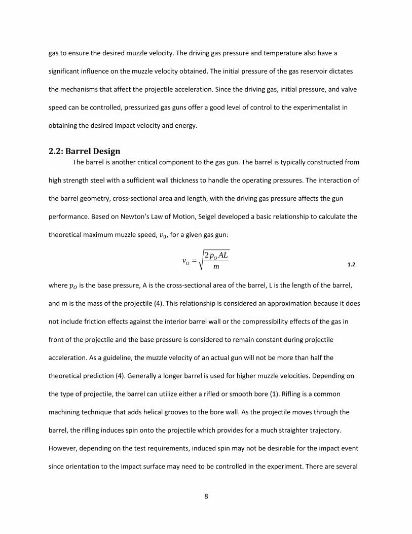
For the final design iteration, a testing program required a spherical steel projectile measuring
1-3/8” in diameter. In order to house the projectile, a larger barrel was necessary. Due to time and
budget constraints, it was determined that the optimum solution was to utilize the basic gun
configuration developed thus far. Therefore the existing gun structure and barrel supports were adapted
to accept the upsized barrel. The upsized barrel configuration was designed such that the
experimentalist could change between the 5/8” bore diameter barrel configuration and the upsized
barrel configuration within one man-hour. The gun in the upsized barrel configuration is shown in Figure
2.9. The nominal inner diameter of the barrel is 1-1/2” and the factor of safety calculated to be 4.80 as
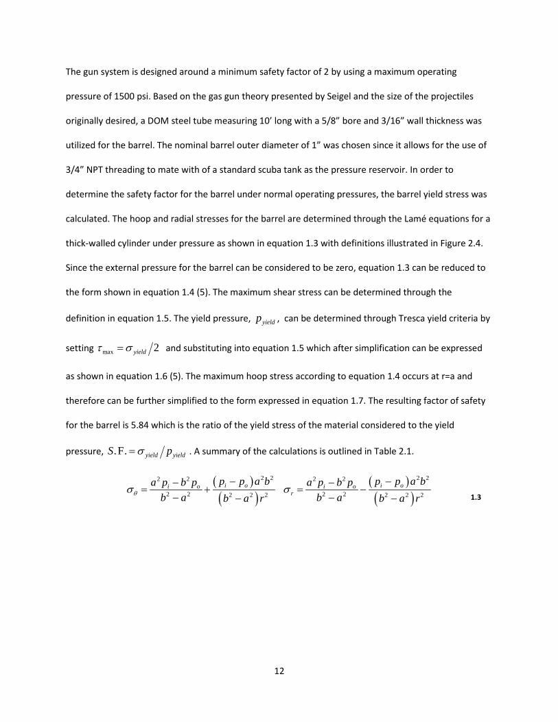
outlined in Table 2.1. The existing barrel supports were also reused. For the larger barrel size, suitable
linear bearings for barrel supports were cost prohibitive. As such bushings were made using Delrin with
DOM steel tube as the bushing housing. The Delrin bushings were manufactured using a lathe and then
press fit into DOM housings. The Delrin bushing assemblies are shown in Figures 2.10 and 2.11 for the
center and end supports, respectively.
17
Figure 2.9: Experimental Gas Gun Upsized Barrel Configuration
Figure 2.10: Upsized Barrel Delrin Bushing; Center Support
18

Figure 2.11: Upsized Barrel Delrin Bushing; End Support
2.5 : Gas Gun Design Performance The gas gun developed during the course of the research is currently capable of impact
velocities ranging from 100 to 800 meters per second. As mentioned in previous sections, the main
impact velocity control mechanisms for the current gun design are the choice of the driving gas and the
initial pressure of the reservoir. As such for each driving gas, air and helium, a performance relationship
can be established for a particular projectile. In order to establish the pressure versus impact velocity
relationship, 1/4” diameter spherical steel projectiles were accelerated using a range of pressures. The
velocities were measured using a high speed video camera as outlined in Chapter 3. As shown in Figure
2.12, a logarithmic regression was used to establish the pressure-velocity relationship for air. Beyond
approximately 600 psi the impact velocity does not increase significantly and plateaus. In addition it is
also apparent that the speed of sound is the limiting factor for the single stage gun design.
19

Figure 2.12: Projectile Velocity As A Function Of Pressure For Air
Performing the same tests using helium as the driving gas resulted in the logarithmic pressure-velocity
relationship illustrated in Figure 2.13. It is easily noticed that the helium easily outperforms air but
unlike air the gas gun was not able to approach the speed sound for helium as closely as in the case of
air. This is likely due to the fact that the barrel is initially filled with ambient air prior to projectile
acceleration. Immediately after the fast-acting valve releases the pressurized helium, the barrel
becomes filled with a mixture of helium and air where the density and thus the speed of sound is
somewhere between that of helium and air. This mixture negatively affects the resulting velocity. As
mentioned in a previous section, a typical countermeasure to increase the velocity obtained at a given
initial pressure of helium is to evacuate the barrel and fill it with helium. Since additional equipment
would need to be implemented and the performance obtained is satisfactory, this countermeasure is
left for future improvement efforts.
20

Figure 2.13: Projectile Velocity As A Function Of Pressure For Helium
Impact location accuracy and precision are part of the design parameters for the gun and also
are highly important in ballistic experiments. By striking in the center of the target for each of the test
shots, the experimentalist can ensure that the effect of the boundary conditions are comparable
between each test and minimizes the chance the boundary conditions affect the resulting data. In Figure
2.14, a location plot of the impact is provided for a test consisting of 13 samples at various velocities in
order to simulate an actual test matrix. The center of the target is at the x and y coordinates of 2.5” and
2.5”, respectively. From visual inspection, both the precision and accuracy of the gun is high. The
standard deviation for the impact locations in both the x and y coordinates are 0.027” and 0.145”
respectively. Reviewing the standard deviations the y coordinate location is less precise but is expected
as the amount the projectile drops is related to the velocity at which it is traveling. The impact locations
21

are no greater than a 0.14” radius from center for a maximum striking zone area of 0.062 𝑖𝑖𝑖𝑖2. Based on
this analysis, the interaction effects between the impact location and the boundary conditions can be
considered constant in experimental testing.
Figure 2.14: Projectile Impact Location
2.6 : Sabot Design Implementation The sabot developed is a three piece push design consisting of three main parts: the two sabot
halves and the interlocking rod. The design can readily handle solids of revolution such as spheres or
cylinders having various impact geometries such as blunt, conical, parabolic, and hemispherical.
Additionally the design can also house asymmetrical geometries effectively. An acetal plastic, known by
the trade name Delrin, was selected as the sabot material based on its strength characteristics, low
friction, and machinability. As can be seen in Figures 2.15 and 2.16, an angled ramp is added to promote
sabot separation through aerodynamic forces. The interlocking rod maintains the positioning of the two
22

halves by preventing relative translation and also provides a pivot point for sabot separation from the
projectile.
Figure 2.15: CAD Representation of Sabot Design With Spherical Projectile
A low cost method, developed by the author, utilizes common machine shop equipment to
create the sabots’ design features. The manufacturing method consists of seven main operations listed
by equipment used and operation description:
1) Lathe - turn down a cylindrical rod of Delrin stock to the appropriate outer diameter
2) Lathe - drill to create the channel to house the projectile
3) Lathe - countersink aerodynamic ramp feature to aid in sabot separation
4) Drill press - drill channel for interlocking rod
5) Miter Saw - precut the sabot to allow for better sabot separation
6) Custom Shear Press - initiate a crack and create two sabot halves
7) Assemble three sabot pieces
23

Figure 2.16: Completed Sabot With Spherical Projectile
The sawing and shear operations are highlighted in Figure 2.17. A custom shear jig was created that
utilizes the mechanical advantage of a drill press to initiate a crack in the Delrin sabot as shown in
Figures 2.18 and 2.19. Additionally the shear jig guides the motion of the cutting blade through the
shearing process. By using a shearing process, no material is lost and the sabot retains its cylindrical
cross section which ensures that proper sealing can be achieved against the barrel bore.
24

Figure 2.17: Assembled Sabot
Figure 2.18: Prototype Shear Jig
25

Figure 2.19: Prototype Shear Jig Mounted In Drill Press
The main benefit to the outlined manufacturing method is that it is readily modified to produce sabots
that can house a wide range of size and geometries. Some of the sabots created for different testing
projects are shown in Figure 2.20.
Figure 2.20: Sample Of Sabots Manufactured
26

2.7 : Sabot Design Validation A high speed video camera was utilized to validate the performance of the sabot. As mentioned
previously, an effective sabot design will accelerate and then separate from the projectile without
affecting the trajectory or inducing trajectory deviations or attitude as illustrated in Figure 2.21. In order
to validate the sabot design, cylindrical rods were shot at approximately 200 meters per second. High
speed video was used to track the sabot and projectile trajectories to evaluate the sabot design.
Cylindrical rods were selected as the evaluation projectile since it is prone to pitch and yaw. Since the
single high speed video camera limits observation to one plane, only projectile pitch will be considered.
Figure 2.21: Projectile Trajectory Deviations, Attitude (Zukas, 1990)
As can be seen in the video stills of Figure 2.22, the sabot starts to separate from the projectile at 3 feet
from the muzzle and is fully separated from the projectile at 4 feet. Through several rounds of
experimentation, the sabot design demonstrated consistent separation from the projectile without
affecting the trajectory or inducing pitch. Also evident from the video stills is that although the sabot
separates from the projectile, the sabot maintains the same general trajectory as the projectile and thus
additional protection is needed to protect the test sample from impact with the sabot. As illustrated in
Figure 2.23, two sabot stripper plates were placed in front of the impact location to ‘strip’ or separate
the sabot from the projectile. The first stripper plate is constructed of 12 gauge sheet steel and the
second plate is a 0.5” thick Lexan plate. Lexan was selected for the second stripper plate to allow for
27

light to illuminate the impact location. Each stripper plate has a hole cut to allow only the projectile to
pass through the plate. The first stripper plate blocks most of the sabot but causes a particle field due to
the fracture of the Delrin upon impact. The second stripper plate blocks the sabot particle field from
impacting the test sample.
Figure 2.22: High Speed Video Stills Of Sabot Design Validation
28

Figure 2.23: Sabot Stripper Plates
29

Chapter 3 : Velocity Measurement In order to establish the energy absorption capabilities of the composite, the velocity of the
projectile both pre- and post-impact must be measured. There are several different methodologies
available which include chronographs, laser array fields, and high speed video cameras. Chronographs
and laser field arrays typically have two gates that are a predetermined distance apart at each point
where velocity needs to be measured. As an object breaks the gate, a timer is started and stopped. The
average velocity over the gate distance is calculated using the elapsed time and the gate distance.
Similarly for a high speed video camera the elapsed time between each of the frames is known and
using a reference distance the instantaneous velocities can be calculated for each frame. Each of the
methods has its advantages and disadvantages. Chronographs and laser arrays calculate the velocity
very close to real time. Thus a near instantaneous velocity readout is obtained. The main problem with
chronographs and laser arrays is that the gates may not sense the object passing and no velocity
calculation will be recorded. High speed cameras not only provide the velocity measurements but may
also provide additional information such as the deflection of the composite panel during impact or the
amount of particulate created due to impact and the particulate dispersion. However high speed video
will result in many frames and require post-processing the images to calculate the velocities. So the
velocity measurement is not produced in real time. All of the aforementioned methods require that
lighting in the area of interest be controlled. For this study, a high speed camera was selected since it is
possible to gain further insight regarding the impact event.
3.1 : High Speed Camera The camera used for the present study is a NAC HotShot 512c shown in Figure 3.1. Its
capabilities include resolutions of 512 x 512 pixels with frame rates up to 200,000 frames per second (6).
The camera can record full resolution frames up to 5,000 frames per second and beyond which the
resolution is reduced to maintain within the camera’s data throughput limitations (6). For the velocities
30

and recording environment in this study, a frame rate of 10,000 frames per second and a shutter speed
of 1/100,000 were found to provide suitable video quality. As mentioned earlier, lighting is a very
important consideration to the video quality possible given a particular recording environment. Since
the safety enclosures do not allow for much ambient lighting to enter, an array of halogen lights were
utilized to illuminate the impact event. Note that special care must be taken to mitigate the level of heat
gain in the composite samples when using halogen lighting due to the heat output. In addition to the
halogen lighting, the interior walls of the safety enclosure were either painted or coated white to take
advantage of the reflectivity provided by the white paint. An example of the resulting images is depicted
in Figure 3.2. It is apparent from the image stills that additional information such as the particulate
distribution can be observed.
Figure 3.1: High Speed Video Camera Used For Velocity Measurements
31

Figure 3.2: High Speed Video Frames From Composite Panel Ballistic Impact
3.2 : Velocity Calculations Using Image Processing As mentioned earlier, velocity calculations using high speed video images requires a reference
distance. Since a digital high speed camera was utilized the cameras’ pixel grid array can be calibrated to
an object. A common technique to obtain calibration is the use of a metric board as pictured in Figure
3.3. The metric board used in the study is a translucent plastic board with gridlines measuring 2” x 1”,
vertically and horizontally, respectively. During calibration, the metric board is placed in the trajectory
path of the projectile and a scaling factor is obtained from the cameras pixel grid array. The camera
software provided by the manufacturer has a built-in feature to facilitate determining the scaling factor.
32

Figure 3.3: Metric Board During Calibration Of High Speed Video Camera
Since the frame rate selected for this research produces a large number of frames to
postprocess for the velocity measurements, the author developed a stand-alone program to better
facilitate velocity calculations of the projectile. The graphical user interface, GUI, of the velocity
calculation program is shown in Figure 3.4.
Figure 3.4: Velocity Calculation Program GUI
The program was written and compiled using the deployment compiler in MATLAB. MATLAB was chosen
since the existing image processing functions could be leveraged in order to expedite the development
of the program. The program can calculate the x- and y-coordinate velocities of the projectile, calculate
33

Coefficient of Restitution or COR, and export the resulting velocity data and processed video files. The
user can select the units of measure for both time and distance.
In order to demonstrate the program flow, an example of a 1/4” steel ball impacting the
composites from the research study will be given. To start the velocity calculation process, the user first
imports the desired video file and trims out unnecessary frames. Next the video frames can be cropped
to eliminate unnecessary pixel data as shown in Figure 3.5. The user can then adjust the pixel contrast
by adjusting the pixel intensity as illustrated in Figure 3.6. The RGB data of the frames are then
converted into black and white data while simultaneously removing image noise. The resulting black and
white images should show the projectile as a white entity. In this case an optional function allows the
user to invert the image as shown in Figure 3.7. Next the image tracking algorithm can be requested by
the user. The algorithm identifies the centroid pixel coordinates of the white entity in each of the video
frame images and the program marks the centroid calculated with an orange-colored marker as shown
in Figure 3.8. Now, depending on the calculations desired, the user can select the x- and y-velocities or
COR to be calculated. Figure 3.9 shows the plot that is outputted from the velocity calculations which in
this example shows an average velocity of 154.5685 meters per second. At this point the user can
choose to export the data used to calculate the velocities. For the majority of the research, the velocity
data was processed in this fashion. However in the case where no perforation occurred and the
projectile deflected back, the COR algorithm could be utilized. In order to demonstrate the COR
calculation algorithm, an example of a baseball impacting a steel plate is analyzed. The COR can be
defined as the ratio of the residual projectile velocity to the initial velocity as shown in equation 2.1.
Re sidual VelocityCORInitial Velocity
= 2.1
Figure 3.10 shows the unprocessed video file image. After processing the image in the same manner as
described for the previous example, the resulting video file appears as illustrated in Figure 3.11. The plot
34

results from the COR calculation algorithm is shown in Figure 3.12 where a COR of 0.5089 is obtained for
an impact velocity of 53.616 miles per hour. The plot also shows the velocities that are averaged to
compute the initial and final velocities. The COR algorithm identifies the minimum acceleration where
the ball bounces back and uses a velocity threshold value inputted by the user to determine the pre- and
post-impact velocities to calculate the COR as shown in Figure 3.13
Figure 3.5: Video Data Trimmed And Cropped
35

Figure 3.6: Pixel Intensity Adjusted
Figure 3.7: Image Inversion
36

Figure 3.8: Centroid Data Calculated For Video Frame Images
Figure 3.9: X- And Y-Velocity Plot Output
37

Figure 3.10: Unprocessed Baseball Impact Video
Figure 3.11: Processed Baseball Impact Video
38

Figure 3.12: COR Output Results
Figure 3.13: COR Algorithm; Determination of Minimum Acceleration
39

Chapter 4 : Composite Panel Ballistic Impact Testing Results Experimental ballistic testing was performed for two different research projects studying
composite material behavior. Previous testing has suggested that a performance differential exists
between thermoplastic and epoxy composites with the same fiber structure and or layup orientation.
Since the data was very limited in those preliminary observations, a more detailed study is needed to
better quantify the performance differential. A formal study comparing the performance differential of
thermoplastic and epoxy based composites subject to ballistic impact was performed. Additionally a
new performance requirement to establish the energy absorption capability for composite structures
subject to a specific falling object hazard requires an experimental test procedure. The test setup is
developed and a preliminary test matrix is tested. The results from the falling object hazard test are
examined for the composite behavior. Areas where improvements can be made in the initial test setup
are identified.
4.1: Introduction Carbon fiber composites are currently being adopted into applications where a combination of
light weight and strength are needed. In many applications such as those in the aerospace sector, the
response to errant fragments and the resulting particle debris field is pertinent to evaluate a potentially
critical failure mode such as the hypervelocity impact of the Columbus module shielding (7) (8). The
kinetic energy of the resulting debris field can also cause further damage to internal components such as
structural elements and control systems. However experimental testing is an expensive process to incur
on several possible designs. In order to reduce the amount of experimental testing needed, considerable
effort is going towards a better understanding of the underlying mechanics involved in terminal ballistics
and accurately modeling the response using numerical methods such as Finite Element methods (9).
In order to properly apply a numerical approach to model the impact event, experimental
testing is needed for model evaluation and validation. One of the common performance characteristics
40

in impact dynamics is the 𝑉𝑉50 or ballistic limit velocity (10) (11). 𝑉𝑉50 is defined as the velocity at which
perforation of the target occurs 50% of the time and as such is considered to be the threshold for the
energy absorption capabilities. There are several different methodologies to develop
𝑉𝑉50 experimentally. The most referenced are the Jonas-Lambert correlation and Recht-Ipson formula as
shown in equations 4.1 and 4.2, respectively (12) (13).
( ) ( )1/22 250 , /RES IMPV a V V a M M m= − = + 4.1
( )1/
50
PP PRES IMPV a V V= − 4.2
Both are based on the conservation of energy but the Jonas-Lambert correlation utilizes a semi-
empirical approach through two correlation factors: a and p (14). A minimum of three experimental data
points are needed in the Jonas- Lambert correlation to solve for the three variables (15). As has been
demonstrated by others, these techniques have difficulty due to the fact that as the 𝑉𝑉50 is approached,
there is a ‘zone of mixed results’ where perforation predictability varies as shown in Figure 4.1 (10) (15)
(16).
Figure 4.1: V50 And The Zone Of Mixed Results (Solsby, 1987)
The methodology used in this research is a variation on the bisection method or also known as
bracketing. Generally the bisection method is the most efficient but can be still problematic in the ‘zone
of mixed results’ (15). The operating principle starts with an initial velocity bracket based on available
41

ballistic data for both composite construction and projectile impact geometry. The first experimental
test is performed at the midpoint value of the initial velocity bracket. If perforation occurs, then a slower
impact velocity will be chosen for the next shot based on the residual velocity, whereas, if perforation
does not occur, then a higher impact velocity will be chosen. A velocity bracket is created in this manner
where the next impact velocity is at the midpoint between the initial estimate and the initial bracket
range. The testing continues until the resulting 𝑉𝑉50 converges within a desired range of error.
4.2 : Ballistic Impact Comparison of Thermoplastic and Epoxy Based Composites
As mentioned earlier the development of the gas gun was performed in conjunction with
Mechanical Engineering undergraduate design teams. In parallel, Polymer Fiber Engineering
undergraduate design teams designed, manufactured, and experimentally tested composites panels.
Part of the experimental testing included high velocity ballistic testing utilizing the developed
experimental gas gun system outlined previously. Several design teams created a range of composite
panels using various constituent materials and layup orientations. During the course of the testing of the
student-produced panels, it was observed that there was a significant performance differential between
epoxy and thermoplastic based composite panels using a 4 x 4 twill woven carbon fiber fabric. Since the
students produced the composites in a manual press where the pressure and temperature had to be
controlled manually during the curing cycle, some of the panels were suspected to be of various levels of
quality in terms of matrix infusion and void presence. This could lead to a higher variation in panel
performance. Also the student teams produced very few panels for each of the experimental tests in
their study which limited the significance of the performance differential observed. As such a more in-
depth analysis was deemed necessary.
A common aerospace grade carbon fiber, T300 five harness satin with a 3k fiber count (T300 5HS
3k), was used as the basis of the comparison. The test matrix proposed for the testing included four
42

different matrix constituents. These included a standard and toughened epoxy, RM2002 and RM2005
respectively, and two thermoplastics, polyphenylene sulfide (PPS) and polyethylenimine (PEI). RM2002
and RM2005 are manufactured by Renegade Materials. The epoxies are similar in formulation to Hexcell
8552 epoxy (17) (18). The thermoplastics were manufactured by Tencate (19) (20). The panels were 12
plies thick or 4.1 millimeters nominally. The layup was orientated in the 0° direction such that the warp
and weft fabric orientations were the same between each ply. In previous rounds of testing, typically a
minimum of five tests were needed to experimentally determine the ballistic limit velocity. For each of
the four constructions, obliquity angles of 0° and 45° were tested. It is well known that the obliquity
angle or angle of the trajectory path to the normal direction of the panel plane will have an effect due to
both geometry considerations and also the resulting asymmetrical stress wave propagation. The test
fixture, as in Figure 4.2, was adjusted appropriately to obtain the desired obliquity angles. Additionally it
should be noted that a standard torque sequence was utilized on the fixture to obtain a uniform
clamping pressure along the boundary condition. The torque sequence moved in a clockwise fashion
where bolts across from each other are tightened. Uneven clamping pressure along the boundary
condition could lead to test panel slippage and also localized crushing which can both have a significant
influence on the test results.
43

Figure 4.2: CAD Representation Of Test Sample Fixture (AMRDEC, 2010)
A total of 48 tests were performed where six panels were tested for each construction/obliquity angle
combination. No replication was used in this study as this would increase the amount of experimental
testing necessary considerably. Thus statistical significance cannot be reported to establish the variance
of the panels tested. Each of the panels measured 6” x 6” (LW) and was constrained by a 0.5”overlap
clamped condition on the perimeter such that the unconstrained portion of the panel measured 5” x 5
(LW). A CAD representation of the test fixture used in experimental testing is shown in Figure 4.2. The
projectile selected for the testing was a 1/4” diameter steel spherical ball bearings. The projectile is
shown with the sabot in Figure 4.3. The testing was performed using the gas gun configuration shown in
Figure 2.5 with the 5/8” bore diameter. Both helium and air were used as driving gases in the
experimental testing.
44

Figure 4.3: 1/4" Diameter Spherical Projectile With Sabot
The summaries of the ballistic results for the RM2005, RM2002, PPS and PEI constructions are in
Tables 4.1, 4.2, 4.3, and 4.4, respectively. The entrance and exit velocities have been normalized relative
to the maximum velocity in each dataset. For each of the constructions and obliquity angles, pre- and
post-impact panel weights and projectile velocities were recorded. The panel weights were used to
quantify the level of mass loss for each of the impact events. The digital weigh scale used has a
resolution of 0.05 grams. The initial and residual velocities were measured using the high speed video
camera as outlined in Section 3.2. The ballistic limit velocities or 50V are calculated by estimating the
intercept of the initial and residual velocities.
From Tables 4.1 and 4.2, the toughened and standard epoxies performance can be compared.
Initially in the testing, it was anticipated that the panels would require velocities well beyond 300
meters per second, thus helium was selected as the driving gas. However from the RM2005 epoxy test
matrix in Table 4.1, helium provided too much energy for the composite panels and projectile
considered. For the remainder of tests, air was used for the driving gas. The calculated ballistic limit
45
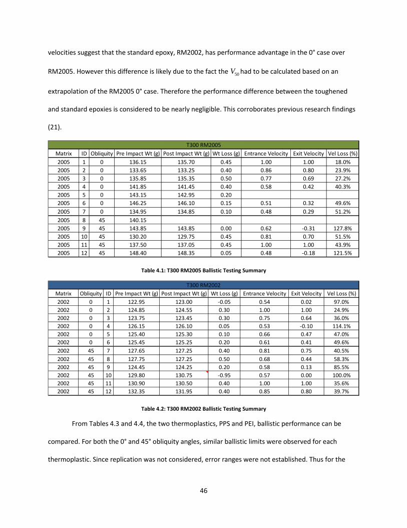
velocities suggest that the standard epoxy, RM2002, has performance advantage in the 0° case over
RM2005. However this difference is likely due to the fact the 50V had to be calculated based on an
extrapolation of the RM2005 0° case. Therefore the performance difference between the toughened
and standard epoxies is considered to be nearly negligible. This corroborates previous research findings
(21).
Table 4.1: T300 RM2005 Ballistic Testing Summary
Table 4.2: T300 RM2002 Ballistic Testing Summary
From Tables 4.3 and 4.4, the two thermoplastics, PPS and PEI, ballistic performance can be
compared. For both the 0° and 45° obliquity angles, similar ballistic limits were observed for each
thermoplastic. Since replication was not considered, error ranges were not established. Thus for the
Matrix ID Obliquity Pre Impact Wt (g) Post Impact Wt (g) Wt Loss (g) Entrance Velocity Exit Velocity Vel Loss (%)2005 1 0 136.15 135.70 0.45 1.00 1.00 18.0%2005 2 0 133.65 133.25 0.40 0.86 0.80 23.9%2005 3 0 135.85 135.35 0.50 0.77 0.69 27.2%2005 4 0 141.85 141.45 0.40 0.58 0.42 40.3%2005 5 0 143.15 142.95 0.202005 6 0 146.25 146.10 0.15 0.51 0.32 49.6%2005 7 0 134.95 134.85 0.10 0.48 0.29 51.2%2005 8 45 140.152005 9 45 143.85 143.85 0.00 0.62 -0.31 127.8%2005 10 45 130.20 129.75 0.45 0.81 0.70 51.5%2005 11 45 137.50 137.05 0.45 1.00 1.00 43.9%2005 12 45 148.40 148.35 0.05 0.48 -0.18 121.5%
T300 RM2005
Matrix Obliquity ID Pre Impact Wt (g) Post Impact Wt (g) Wt Loss (g) Entrance Velocity Exit Velocity Vel Loss (%)2002 0 1 122.95 123.00 -0.05 0.54 0.02 97.0%2002 0 2 124.85 124.55 0.30 1.00 1.00 24.9%2002 0 3 123.75 123.45 0.30 0.75 0.64 36.0%2002 0 4 126.15 126.10 0.05 0.53 -0.10 114.1%2002 0 5 125.40 125.30 0.10 0.66 0.47 47.0%2002 0 6 125.45 125.25 0.20 0.61 0.41 49.6%2002 45 7 127.65 127.25 0.40 0.81 0.75 40.5%2002 45 8 127.75 127.25 0.50 0.68 0.44 58.3%2002 45 9 124.45 124.25 0.20 0.58 0.13 85.5%2002 45 10 129.80 130.75 -0.95 0.57 0.00 100.0%2002 45 11 130.90 130.50 0.40 1.00 1.00 35.6%2002 45 12 132.35 131.95 0.40 0.85 0.80 39.7%
T300 RM2002
46

purpose of the study, the difference in ballistic performance between PPS and PEI will be considered
small to negligible. A larger study will be needed to better quantify the difference between the two
thermoplastics.
Table 4.3: T300 PPS Ballistic Testing Summary
Table 4.4: T300 PEI Ballistic Testing Summary
The ballistic data for the epoxies and thermoplastics in Tables 4.1, 4.2, 4.3, and 4.4 can be
reorganized for graphical plot comparison. Based on the results obtained previously, a negligible
performance difference is assumed within each matrix class: epoxies and thermoplastics. Therefore the
data and plots are organized to compare the matrix classes. The 0° and 45° obliquity cases are illustrated
in Figures 4.4 and 4.5, respectively, using the normalized velocity data. It is readily apparent that the
Matrix Obliquity ID Pre Impact Wt (g) Post Impact Wt (g) Wt Loss (g) Entrance Velocity Exit Velocity Vel Loss (%)PPS 0 1 160.00 159.85 0.15 1.00 1.00 35.5%PPS 0 2 159.50 159.55 -0.05 0.70 0.00 100.0%PPS 0 3 160.45 160.45 0.00 0.51 -0.15 118.9%PPS 0 4 160.15 160.15 0.00 0.83 0.51 60.4%PPS 0 5 160.05 159.95 0.10 0.62 -0.17 117.5%PPS 0 6 160.40 160.35 0.05 0.83 0.52 59.9%PPS 45 7 160.95 160.85 0.10 0.91 0.25 85.3%PPS 45 8 158.40 158.35 0.05 0.86 0.31 80.8%PPS 45 9 158.75 158.45 0.30 1.00 1.00 45.6%PPS 45 10 158.65 158.45 0.20 0.94 0.77 55.2%PPS 45 11 160.25 161.35 -1.10 0.82 0.00 100.0%PPS 45 12 159.65 159.55 0.10 0.78 -0.28 119.1%
T300 PPS
Matrix ID Obliquity Pre Impact Wt (g) Post Impact Wt (g) Wt Loss (g) Entrance Velocity Exit Velocity Vel Loss (%)PEI 1 0 159.30 158.85 0.45 1.00 1.00 37.4%PEI 2 0 159.75 159.55 0.20 0.74 0.09 92.8%PEI 3 0 157.25 157.25 0.00 0.60 -0.14 114.5%PEI 4 0 159.35 158.95 0.40 0.90 0.78 45.9%PEI 5 0 160.05 159.80 0.25PEI 6 0 160.15 160.25 -0.10 0.71 -0.12 110.5%PEI 7 45 159.65 159.15 0.50 0.84 0.59 57.6%PEI 8 45 160.05 159.45 0.60 0.76 0.36 71.3%PEI 9 45 159.95 159.85 0.10 0.66 -0.05 105.0%PEI 10 45 159.95 159.55 0.40 0.85 0.58 58.2%PEI 11 45 157.35 156.80 0.55 1.00 1.00 39.3%PEI 12 45 157.05 156.60 0.45 0.79 0.56 57.4%
T300 PEI
47

ballistic limit velocity is noticeably different between the thermoplastic and epoxy matrices. Regardless
of the obliquity angle used, the thermoplastics outperform the epoxies by approximately 10%.
Figure 4.4: 0° Obliquity Ballistic Performance Thermoplastic And Epoxy Comparison
Figure 4.5: 45° Obliquity Ballistic Performance Thermoplastic And Epoxy Comparison
4.3 : Falling Object Hazard, Ballistic Impact With Large Diameter Projectiles Up to this point the majority of the testing has been performed with emphasis on examining the
perforation of composite panels with small projectiles. A new test requirement was needed to establish
the energy absorption of composite panels to an impact of a 6 ounce, 1-3/8” diameter steel sphere
48

traveling at an initial velocity of 150 feet per second. The test is intended to simulate a falling object
hazard for composite structures. In the test, penetration and indentation may occur but it is expected
that the composites will not be perforated. In order to facilitate testing, the gun was modified to handle
the larger projectile as outlined in Figure 2.9. The sabot design and manufacturing process defined in
Section 2.6 were modified in order to handle the larger projectile. The resulting sabot with the projectile
is shown in Figure 4.6. The assembled sabot with the 1-3/8” diameter projectile is shown in Figure 4.7. In
order to keep testing costs low and to avoid special machining, a standard ball bearing was used for the
experimental testing. Figure 4.9 shows early sabot development while testing a composite sample at
approximately 658 feet per second. The video demonstrates that the operating principles of the sabot
translate to the larger design to provide a controlled trajectory. Machining for the large sabot was
slightly more difficult and thus made obtaining a good fit in the barrel bore more challenging. In order to
compensate for the machining difficulties, layers of masking tape were applied on the sabot interior.
The layered tape, as shown in Figure 4.6, provided the additional gauge to ensure good sealing in the
barrel bore and therefore provide repeatable gun performance in both projectile velocity and trajectory.
Figure 4.6: 1-3/8" Spherical Sabot
49

Figure 4.7: Assembled 1-3/8" Spherical Sabot With Projectile
Figure 4.8: CAD Representation Of Large Projectile Test Fixture (AMRDEC, 2012)
50

Figure 4.9: High Speed Video Stills Of Large Projectile Sabot Development; 658 fps
Since the test fixture for previous testing would place the boundary condition too close to the
impact area, a larger test fixture was developed. Figure 4.8 shows the CAD representation of the large
test fixture. The fixture is a larger version of the previous design. It also allows for obliquity angles of 0°
and 45°. The intended panel size for the fixture is 12” x 12” (LW) with the same 0.5” overlap clamped
condition along the perimeter. The free portion of the panel measures 11” x 11” (LW). The same
standard torque sequence mentioned previously is utilized for the large test fixture to ensure even
clamping pressure. The floor of the safety enclosures were further reinforced to minimize the amount of
51

deflection anticipated from the larger mass of the projectile and the mechanical advantage from the
larger test fixture.
A limited test matrix was performed to compare quasi-isotropic layup carbon fiber/epoxy and
carbon fiber/nylon composite panels to a reference of aluminum (AL6061). Since the testing is currently
in the preliminary phases, this round of testing is performed with the intent of establishing the baseline
material performance in addition to evaluation of the test itself. For each of the three materials, four
tests were performed where different thickness samples were tested to an impact of approximately 150
feet per second with the large projectile. In order to consistently obtain an initial projectile velocity of
150 feet per second, air was chosen as the driving gas. Additionally the assembled sabot, as in Figure
4.7, was fitted prior to each test and gauge was adjusted using the layers of tape mentioned previously.
A summary of the results for the considered materials is outlined in Table 4.5.
Table 4.5: Large Projectile Impact Test Summary
Velocities were measured using the methods outlined in Section 3.2. The coefficient of restitution (COR)
for each of the test cases were also calculated using the analysis software developed. As expected, the
COR for the composites have an inverse relationship with respect to the thickness of the composites
such that the COR increases as the thickness decreases. This phenomenon is mainly due to what is
commonly referred to as the ‘trampoline’ effect. As the material becomes thinner, the material starts to
behave more like a trampoline and will more readily deform and deflect impact. As the thickness
Test # Panel Thickness, in Initial Velocity, fps Residual Velocity, fps COR Initial Weight, gr Residual Weight, gr1 Aluminum 0.10 178.14 -58.35 0.3282 Aluminum 0.10 171.76 -54.29 0.3163 Aluminum 0.09 150.20 -51.45 0.3434 Q-I-Epoxy 0.51 158.52 -31.48 0.1995 Q-I-Epoxy 0.39 156.38 -44.54 0.285 1359.20 1359.206 Q-I-Epoxy 0.26 157.99 -65.29 0.413 912.45 912.457 Q-I-Epoxy 0.13 159.88 -81.80 0.512 461.65 461.658 Carbon/Nylon 0.42 157.51 -24.72 0.157 1354.05 1354.059 Carbon/Nylon 0.30 161.12 -32.24 0.200 939.90 938.96
10 Carbon/Nylon 0.20 162.73 -44.43 0.273 591.55 591.3511 Carbon/Nylon 0.10 155.81 -60.20 0.386 336.45 336.3512 Aluminum 0.09 160.33 -52.59 0.328
52

increases, the panel becomes stiffer and deforms less. Therefore more energy is absorbed through the
increased stiffness and mass and also internal damage mechanisms such as delamination and matrix
cracking. Figure 4.10 compares the relationship of COR with respect to the sample thickness. For the
samples considered the quasi-isotropic carbon fiber composite mechanically dissipates more of the
projectile energy evident by the higher COR values for comparable sample thicknesses. Meanwhile the
carbon/nylon composite absorbs more of the projectile energy.
Figure 4.10: COR As Function Of Sample Thickness
The modifications made to the gun configuration allowed for simulation of the falling object
hazard. However some issues were noticed with the test fixture developed. During testing at the
prescribed impact velocity, noticeable deflection was observed in the test fixture. The majority of the
deflection of the test fixture resulted from the mid-span flexure. The progression of the flexure during
impact for test 6 is shown in Figure 4.11. The arrows highlight the flexure where both bending and
twisting is observed. Additionally the test fixture deflected due to flexure in the safety enclosure despite
the reinforcements installed prior to testing. It is unclear the level of influence the test fixture flexure
has on the composite response. A formal study could be performed to quantify the influence of the test
fixture flexure has on the composite response. Based on the observed performance of the test setup,
53

several improvements are suggested for future falling object hazard testing. The test fixture needs a
higher level of rigidity which can be obtained by using thicker plates for clamping the plate or by
switching to steel from the aluminum currently used. Also further reinforcement is needed for the safety
enclosure floor.
Figure 4.11: Test Fixture Mid-span Deflection
54

Chapter 5 : Viscoplastic Composite Model The plasticity framework can effectively be used to describe the nonlinear, rate-dependent
behavior observed in composites. A viscoplastic material model is presented that is suitable for a wide
range of composites under various loading conditions. The model makes no assumption regarding
whether plasticity can form in the fiber axial direction. A return mapping integration scheme is
presented suitable for the viscoplastic material model. Since the model requires more parameters than
the models typically used in the literature, an optimization algorithm has been developed to determine
the parameters for the viscoplastic model. Finally the model is considered for a unidirectional carbon
fiber composite presented in the literature. The model results are compared to the published
experimental data.
5.1 : Development of Sun’s Plastic Potential The associated flow rule is stated as shown in equation 5.1 where f is the plastic potential
function and dλ is the proportionality factor (22). The associated flow or normality flow rule implies
that the plastic strain formation is in normal direction from the yield surface (23). The term associated is
due to the fact that the flow rule and yield criterion are the same functions (23).
pij
ij
fd dλ∂ε =
∂σ
5.1
Hill proposed a generalized orthotropic plastic potential based on the von Mises’ J2 plasticity
theory where the Baushinger effect was ignored and that the addition of hydrostatic loading has no
influence on yielding, the plastic potential, or yield criterion (24). The form of Hill’s plastic potential
takes the form shown in equation 5.2. The expression is equivalent to von Mises’ criterion when
F G H= = and 3L M N F= = = (24).
( ) ( ) ( )2 2 2 2 2 222 33 33 11 11 22 23 31 122 ( ) 2 2 2ijf F G H L M Nσ = σ − σ + σ − σ + σ − σ + σ + σ + σ 5.2
55

Based on Hill’s plastic potential, Sun and Chen proposed a more generalized form of the orthotropic
plastic potential shown in equation 5.3 which did not have the restriction of no plasticity due to
hydrostatic loading (22).
2 2 211 11 22 22 33 33
12 11 22 23 22 33 13 11 332 2 2
44 23 55 13 66 12
2 ( )2 2 2
2 2 2
ijf a a aa a aa a a
σ σ σ σ σ σ
σ = σ + σ + σ
+ + +
+ σ + σ + σ
5.3
Sun and Chen originally formed a 2-D viscoplastic model where the simplifying assumptions were that
no plastic strain occurred along the fiber direction, no plasticity forms due to dilatation, and transverse
isotropic behavior (22). Equation 5.4 is the form derived for the plastic potential where 22 1a = (22).
2 222 22 66 122 ( ) 2ijf a aσ = σ + σ
5.4
Chen et al observed that in effect by making the aforementioned simplifications the derived plastic
potential for the special case of transverse isotropy is equivalent to Hill’s (25). Chen et al further
illustrated that for some cases, such as the example of Boron-Aluminum examined, exhibit plasticity
under uniform dilatation (25). Thiruppuzhi and Sun applied the form of the Sun and Chen’s 2-D
viscoplasticity model shown in equation 5.4 to an Abaqus Finite Element material model for strain rates
from 0.0001 to 1.0 per second (26). Using the recommendations made by Ninan et al, Tsai and Sun
performed a comprehensive analysis on the model by performing off-axis compressive Split Hopkinson
Bar testing at various angles and compared the determined plastic potential coefficients and parameters
for low strain rate and those determined from strain rates ranging from 400 to 1000/s (27) (28). Tsai and
Sun found that the low strain rate parameters could be applied to higher strain rate loadings and
produce good model results (28). Weeks and Sun proposed a 3-D viscoplastic model using the same
assumptions made by Sun and Chen where the plastic potential takes the form shown in equation 5.5
and compared the model to experimental data for strain rates ranging from 10e-6 to 1000 per second
from servo-hydraulic and Split Hopkinson testing (29). The Split Hopkinson testing was performed from
56

100 to 1000 per second on balanced angle ply composites (29). Weeks and Sun obtained good results
from the 3-D viscoplasticity model and posited that the model could also be applied to determine the
off-axis behavior (29).
( ) ( )2 2 2 222 33 23 66 13 122 ( ) 4 2ijf aσσ = σ − σ + + σ + σ 5.5
Recently Flesher et al applied the aforementioned 3-D viscoplastic model to carbon fiber triaxial braided
composites tubes for dynamic crush simulations (30) (31) (32). A simple micromechanical model was
implemented where the axial tows were assumed to have no undulation and took into account the
‘scissoring’ effect of triaxial composites. Flesher also developed a new procedure to determine the 𝑎𝑎66
parameters through the use of rail-shear test data (31). Janapala et al also have recently have expanded
upon Flesher’s work by developing a more generalized form of the plastic potential to model the
behavior of Kevlar braided tubes to dynamic crush, although the actual form of the adopted plastic
potential was not reported (33). As noted by Janapala et al, the original assumptions that plastic strain
did not occur in the tow direction is no longer applicable due to both the rate dependency and plastic
behavior of Kevlar (33). This is readily apparent in the tensile Split Hopkinson testing from the work of
Wang et al for Kevlar fiber bundles reproduced in Figure 5.1 (34). From the positive initial results,
Janapala et al posited that the model was suitable and could be applied to impact analysis (33).
Figure 5.1: Stress-strain curves of Kevlar 49 fiber bundles, Wang et al (34)
57

5.2: Derivation of Viscoplastic Model In the scope of the present work, a more generalized version is desired to represent behavior of
a wider range of composites constituents. In order to be suitable for more fiber types, some of the
plasticity potential constraints such as the lack of plasticity forming along the axis of the tow are
removed.
Chen and Sun later revisited the Hill type plastic potential and derived a new form based on the
finite element results from a representative volume element (RVE) of a square packed array composite
fiber (35). Based on the RVE study, the following observations were made:
a) ‘Plastic strains are compressible and plastic behavior occurs due to hydrostatic stresses’
b) ‘Uniform dilatation does not have an impact on plastic behavior’
c) ‘Behavior along the fiber direction is essentially linear elastic.’
Chen et al noted that to enforce observation ‘b’ the following relation in equation 5.6 results due to the
fact that under uniform dilation 11 22 33ε ε ε ε= = = .
( )( )( )
11 11 12 13
22 12 22 23
33 13 23 33
11 22 33
11 12 13 12 22 23 13 23 33
ij
C C C
C C C
C C C
C C C C C C C C Cwhere C are components of the elastic stiffness matrix
σ ε
σ ε
σ εσ σ σ
= + +
= + +
= + +
= =+ + + + + +
5.6
From the original form of the plastic potential in equation 5.3 and applying the relation in equation 5.6,
a new form of the plastic potential was derived as presented in equation 5.7 (35). This form of the
plastic potential will be utilized in the development of the viscoplastic model since it is a more
generalized form. Additionally the ijα terms can be defined explicitly without the definitions in equation
5.7 to allow for more anisotropic plastic behavior.
58

( ) ( ) ( )2 2 212 11 12 22 23 22 23 33 31 33 31 11
2 2 244 23 55 13 66 12
11 12 13 12 22 23 13 23 3312 23 31
12 22 23 13 23 33 11 12 13
2 ( )
2 2 2ijf A A A
a a awhere
C C C C C C C C CC C C C C C C C C
σ α σ σ α σ σ α σ
σ σ σ
α α α
σ = − + − + −
+ + +
+ + + + + += = =
+ + + + + +
5.7
Chen and Sun observed that although the ijα terms do not equal, Hill’s original plasticity
potential can be obtained by setting the ijα terms equal to unity (35). Also implicit to this plastic
potential is the fact that the initial plasticity is related to the elastic behavior through the ijα terms. As
will be demonstrated in the following section, this feature will be important for modeling highly
anisotropic behavior such as that present in carbon fiber composites when the simplification of linear
elastic axial behavior is not enforced.
Although the form of the plastic potential in equation 5.7 will be used throughout the research,
it is instructive to show that the plastic potential can be simplified for transversely isotropic behavior
present in unidirectional composites. As Hill originally stated, for the case of transversely isotropic
behavior, the plastic potential must remain invariant for an arbitrary rotation about the normal direction
of the isotropic plane (24). Considering the 1-direction to be the direction of the tows, it can be shown
that the following relations in equation 5.8 result from an arbitrary rotation about the 1-axis.
2 212 13 31 13 12 12 55 66A A A A a aα α= = =
5.8
Additionally for transversely isotropic materials the following stiffness matrix components relations can
be applied, 12 13 22 33C C C C= = , resulting in the simplifications to the ijα terms as shown in equation
5.9.
11 12 12 22 23 12 22 2312 23 31
12 22 23 12 22 23 11 12 12
2 112
C C C C C C C CC C C C C C C C
α α αα
+ + + + += = = = =
+ + + + +
5.9
59

Applying the simplifications from equations 5.8 and 5.9 with further algebraic manipulation, the plastic
potential simplifies to the following simplified form.
( ) ( ) ( )( )
2 2 212 11 12 22 23 22 33 12 11 12 33
2 2 244 23 66 13 12
2 ( )
2 2ijf A A A
a a
σ α σ σ σ σ α σ
σ σ σ
σ = − + − + −
+ + +
5.10
The anisotropic terms control the level of anisotropic plastic behavior exhibited by the material.
Through work equivalence, the increment of plastic work per unit volume, PdW , can be
expressed in terms of the stress and plastic strain increment tensors (22). By substituting the associated
flow rule from equation 5.1 into 5.11, the incremental plastic work takes the form shown in equation
5.12. Additionally PdW can also be expressed in terms of the effective stress, σ , and the effective
plastic strain increment, pdε (22).
P pij ijdW dσ ε=
5.11
Pij
ij
fdW dσ λσ∂
=∂
5.12
P pdW dε= σ 5.13
From expansion of equation 5.12, it is apparent that the incremental plastic work is equal to the plastic
potential as shown in equation 5.14.
( )2P pij ij ij ij
ij
fdW d d fσ ε σ λ σσ∂
= = =∂
5.14
After further manipulation of equation 5.14, the proportionality factor can be expressed in terms of σ
and pdε (22). Also the incremental plastic strain can be expressed as shown in equation 5.16. Upon
evaluation of the aforementioned expression, the effective plastic strain increment for the generalized
model, equation 5.7 takes the form shown in 5.17
60

( )( )
3 322
pij p
ij
f dd df
σ ελ εσ
= =σ
5.15
23
pijp
ij
dd f
εε
σ=
∂∂
5.16
( ) ( ) ( )1
2 2 22 2 2
2 12 1 3 23 2 1 31 3 12 23 132 2 2
12 12 23 23 31 31 66 44 55
23 2 2 2
p p p p p p p p pp d d d d d d d d dd
A A A a a aε α ε ε α ε ε α ε ε ε εε
α α α
− − − = + + + + +
5.17
In a similar fashion as the derivation by Thiruppukuzhi, the rate forms of the proportionality factor and
effective plastic strain, equations 5.15 and 5.17 respectively, are expressed as follows. Also, the
viscoplastic modulus term is introduced at this point, PΗ (26) .
3 32 2
p
P pP
whereελε
σ σ= = Η =
σ Η σ
5.18
( ) ( ) ( )1
22 2 22 2 2
2 12 1 3 22 2 1 31 3 12 23 132 2 2
12 12 23 23 31 31 66 44 55
23 2 2 2
p p p p p p p p pp
A A A a a aε α ε ε α ε ε α ε ε ε εε
α α α
− − − = + + + + +
5.19
As Hill and Sun stated, the effective stress can be expressed as the following form (22) (24).
3 fσ = 5.20
Evaluating the expression in equation 5.20 with the plastic potential from equation 5.10, the effective
stress for the two parameter model takes the form shown in equation 5.21.
( ) ( ) ( )
1222 2
12 11 12 22 23 22 23 33 31 33 31 11
2 2 266 12 44 23 55 13
32 2 2 2a a a
σ α σ α σ α σ
σ
Α − + Α σ − σ + Α − σ = + σ + + σ
5.21
The effective stress rate is found by taking the derivative of equation 5.21 with respect to time. After
simplification and reordering the effective stress rate equation can be represented as shown in 5.22.
61

( ) ( )( )( ) ( )( )( ) ( )( )
12 11 12 22 31 31 33 31 11 11
23 22 23 33 12 12 11 12 22 22
31 33 31 11 23 23 22 23 33 33
66 12 12 44 23 23 55 13 13
( ) 32
2 2 2
ddt
a a a
α σ α α σ
α σ α α σσσ α σ α α σ
σ σ σ σ
Α σ − − Α σ − σ + Α σ − − Α σ − σ σ = = + Α σ − − Α σ − σ + + + σ σ
5.22
As noted from Sun, fiber composites experimentally do not exhibit a definite yield point so a
simple power law was used to fit the master effective stress - effective strain curve as shown in equation
5.23. The master effective stress- effective strain curve is developed from off-axis testing. Thiruppukuzhi
expanded the power law such that the coefficient Α is a power law of the effective plastic strain rate as
shown in equation 5.24. Applying the aforementioned power laws, the viscoplastic modulus can be
expressed as shown in equation 5.25. As noted by Flesher there can be several suitable nΑ, pairs and
thusly proposed and implemented a relationship established from the monotonic loading conditions
present in a rail-shear test (31). The terms χ and m are denoted the viscoplasticity terms (26). χ and m
are determined by plotting the log-log relation of Α and the effective plastic strain rate where they are
the intercept and slope, respectively (26). As evidenced by the power law, χ has a linear effect on the
material behavior (31). m controls the rate sensitivity of the material (26). Negative values of m
correspond to stiffening behavior as load rate increases which is often observed in polymeric
composites (31). The n term controls the shape of the power law curve fit (31).
p nε σ= Α 5.23
( ) ( )m mp p p nA χ ε ε χ ε σ= = 5.24
( ) ( ) 1
1P mp npnε χ ε σ −
σΗ = =
5.25
Since this material model will be implemented into an explicit integration Finite Element code
where many small time steps are made, the small strain assumption can be made and the strain rate can
62

be additively decomposed into elastic and plastic contributions (36). By evaluating the additive
decomposition strain rates, and likewise strain, in equation 5.26, the strain rate-stress rate relationship
can be considered to be a function of the elastic and viscoplastic compliance matrices, ES and VPS
respectively, shown in equation 5.27.
{ } { } { }e pε ε ε= + 5.26
{ } { },TOT TOT E VPS where S S Sε σ = = + 5.27
The elastic compliance matrix for transversely isotropic materials can be expressed as shown in equation
5.28 (37). Note that the order of the compliance matrix is the nonstandard order utilized by LS-DYNA
and this order will be used throughout the present study.
11 12 13
12 22 23
13 23 33
44
55
66
131211 12 13
1 1 1
2322 23 33
2 2 3
44 55 6612 23 13
0 0 00 0 00 0 0
0 0 0 0 00 0 0 0 00 0 0 0 0
1
1 1
1 1 1
E E E
E E E
E E EE
E
E
E
E E E
E E E
E E E
S S SS S SS S S
SS
SS
where
S S SE E E
S S SE E E
S S SG G G
νν
ν
=
−−= = =
−= = =
= = =
5.28
Considering the rate form of the associated flow rule in equation 5.29 and applying equations 5.18, and
5.25, the viscoplastic compliance matrix can be determined as defined explicitly in equations 5.30-5.32.
pij
ij
f λ∂ε =
∂σ
5.29
63

1111
2222
3333
1212
2323
1313
p
p
pVPijp
p
p
S
εεε
σ σ σ = τγ τγ
τγ
5.30
( ) ( )
11 12 13 14 15 16
12 22 23 24 25 263
13 23 33 34 35 36
14 24 34 44 45 46
15 25 35 45 55 56
16 26 36 46 56 66
94
VP VP VP VP VP VP
VP VP VP VP VP VP
m np VP VP VP VP VP VPVP
VP VP VP VP VP VP
VP VP VP VP VP VP
VP VP VP VP VP VP
S S S S S S
S S S S S S
n S S S S S SS
S S S S S S
S S S S S S
S S S S S S
χ ε σ −
=
5.31
( )
2 211 12 13 14 15 16 22
223 24 25 26 33 34 35
2 2 236 44 45 46 55 56 66
212 31 31 11 12 12 22
VP VP VP VP VP VP VP
VP VP VP VP VP VP VP
VP VP VP VP VP VP VP
S A S AB S AC S AD S AE S AF S BS BC S BD S BE S BF S C S CD S CES CF S D S DE S DF S E S EF S F
where
A α α σ
= = = = = = == = = = = = == = = = = = =
= Α + Α σ − Α −
( )( )
31 31 33 66 12
212 12 22 23 12 12 22 23 23 33 44 23
231 31 11 23 23 22 31 23 23 33 55 13
2
2
2
D a
B E a
C F a
α σ
α σ α α σ σ
α σ α σ α
Α = σ
= −Α + Α + Α σ − Α =
= −Α − Α + Α + Α σ = σ
5.32
5.3 : Return Mapping Algorithm In general solving the 1st order ordinary differential equations represented by equations 5.29
through 5.32 explicitly will result in a conditionally stable solution which requires a sufficiently small step
to maintain numerical stability. Since it is expected that large strain increments may occur in the ballistic
impact simulations, a return mapping algorithm based on a 1st order backward Euler integration
algorithm will be utilized to obtain unconditional stability (38). Additionally, as pointed out by Simo et al,
the return mapping algorithm transforms the differential equations into an algebraically constrained
optimization problem (38). An example of the general class of return mapping algorithms is the well-
known radial return integration scheme for J2-plasticity proposed by Key and Krieg (39). Return mapping
64

integration schemes are based on the split operator methodology where the elastic and plastic
components of the material response are split into a predictor-corrector scheme (38) (39). The most
common split is the elastic predictor/plastic corrector but Fotiu et al have also proposed a plastic
predictor/elastic corrector scheme (40). For the elastic predictor/plastic corrector split, the elastic
prediction is returned to the plastic yield surface which is convex due to the associated flow rule utilized.
Ortiz and Simo formulated the generalized algorithm for rate-independent elastoplastic material
behavior (41). Return mapping algorithms have also been extended to viscoplastic constitutive behavior
using overstress functions such as the Duvaut-Lions and Perzyna models and also rate tangent modulus
method (38) (39). Wang et al have proposed a consistency model for rate-dependent elastoplastic
models that uses the consistency condition that results from the Kuhn-Tucker or loading/unloading
conditions, equation 5.33 (42), where F denotes the plastic yield function.
0 0 0
( , , ) 0
F Fwhere
F
λ λ
σ λ λ
≥ ≤ ≤
=
5.33
Since the associated flow rule and hardening rule have been implemented, the algorithm
outlined by Wang et al is applicable and will be utilized for the present research. From equation 5.33,
the consistency condition can be expressed as shown in 5.34. The summarization of the general
algorithm is shown in Figure 5.2 where n and k refer to the global and the local solution steps,
respectively (42). It should also be noted that a slight modification was made to the algorithm to be able
to use the dual power law hardening rule shown in equation 5.24. In order to obtain a continuous
solution the power law requires that the instantaneous viscoplastic scaling factor rate, λ , must be
initialized to the value at the previous time step. This relaxes the split operator definition which states
that the plastic evolution is frozen during the elastic predictor.
65

( , , ) : 0F F FF σ λ λ σ λ λ
σ λ λ∂ ∂ ∂
= + + =∂ ∂ ∂
5.34
( )
( )
1 1
1
0 0 0 0 0 01 1 1 1
12
2
, 0;
0 , ,
En tr n n
tr n
k k k k k kn n n tr tr n n
th
k E k
Tk k
Calculate Elastic PredictorC
if F plastic state
Initialize
F F
Begin k iteration
FH S
F FH
ε σ σ ε
σ λ
λ λ λ σ σ σ λ λ
λσ
β λσ σ
+ +
+
= = = = = =+ + + +
−
∆ = + ∆
≥
∆ = = = =
∂= + ∆ ∂
∂ ∂ = + ∆ ∂ ∂
2 2
1
1 11 1
11 1
1
1
1
, ,
,;
kk
kk k
k
k E kn n n
kk k
tr n
k
n tr
F F F Ft t
F
FC
F Ft
if F tol perform next iterationelse elastic state
λσ λ λσ λ λ
λ λβ
σ σ ε λσ
λσ λ λ
σ σ
+
+ ++ +
++ +
+
+
∂ ∆ ∂ ∂ ∂+ − − ∂ ∂ ∆ ∂ ∆∂ ∂ ∂
∆ = ∆ +
∂ = + ∆ − ∆ ∂ ∆
= + ∆ ∆ >
=
Figure 5.2: 3-D General Return Mapping Algorithm
Up to this point the general orthotropic model presented in the previous section has been
stated in the quadratic form, equation 5.7. For the return mapping algorithm, the yield function, F, can
be stated in terms of the effective stress as shown in equations 5.35 since pλ ε= through work
equivalence. The 1st partial derivatives and 2nd partial derivatives, or Hessian matrix, of the yield
function, F, for the return mapping algorithm can be defined explicitly as shown in equations 5.36 and
5.37. It can be observed that the Hessian matrix defined in equation 5.37 is symmetric.
66

( )
( ) ( ) ( )
( )( )
1222 2
12 11 12 22 23 22 23 33 31 33 31 11
2 2 266 12 44 23 55 13
1
( , , ) , 0
32 2 2 2
,
p p p p
np
p pmp
F
where
a a a
σ ε ε σ σ ε ε
σ α σ α σ α σ
σ
εσ ε εχ ε
= − =
Α − + Α σ − σ + Α − σ = + σ + + σ
=
5.35
{ }
( )
( )
( )( )
1
1
212 31 31 11 12 12 22 31 31 33 66 12
212 12 22 23 12 12 22 23 23 33 44 23
31 31 11 23 23 22 31 23 2
32
1
2
2
T
np
mp p p
np
mp p p
F A B C D E F
Fn
F mn
where
A D a
B E a
C
σ σ
εε ε χ ε
εε ε χ ε
α α σ α σ
α σ α α σ σ
α σ α σ α
∂=
∂
∂ = − ∂
∂ = ∂
= Α + Α σ − Α − Α = σ
= −Α + Α + Α σ − Α =
= −Α − Α + Α + Α
( )23 33 55 132F aσ = σ
5.36
67

2 2 2 2 2 2
21 2 1 3 1 12 1 23 1 13 1
2 2 2 2 2 2
22 1 2 3 2 12 2 23 2 13 22 2 2 2 2 2
2 23 1 3 2 3 12 3 23 3 13 32 2 22
12 1 12 2 12
F F F F F F
F F F F F F
F F F F F FF
F F F
σ σ σ σ σ σ σ σ σ σ σ
σ σ σ σ σ σ σ σ σ σ σ
σ σ σ σ σ σ σ σ σ σ σσ
σ σ σ σ σ
∂ ∂ ∂ ∂ ∂ ∂∂ ∂ ∂ ∂ ∂ ∂ ∂ ∂ ∂ ∂ ∂∂ ∂ ∂ ∂ ∂ ∂
∂ ∂ ∂ ∂ ∂ ∂ ∂ ∂ ∂ ∂ ∂∂ ∂ ∂ ∂ ∂ ∂
∂ ∂ ∂ ∂ ∂ ∂ ∂ ∂ ∂ ∂ ∂ ∂=∂ ∂ ∂∂
∂ ∂ ∂ ∂ ∂ ∂
2 2 2
23 12 23 12 13 12
2 2 2 2 2 2
223 1 23 2 23 3 23 12 23 13 232 2 2 2 2 2
213 1 13 2 13 3 13 12 13 23 13
2
21
3
F F F
F F F F F F
F F F F F F
where
F
σ σ σ σ σ σ
σ σ σ σ σ σ σ σ σ σ σ
σ σ σ σ σ σ σ σ σ σ σ
σ
∂ ∂ ∂
∂ ∂ ∂ ∂ ∂ ∂ ∂ ∂ ∂ ∂ ∂ ∂ ∂ ∂ ∂ ∂ ∂ ∂ ∂ ∂ ∂ ∂
∂ ∂ ∂ ∂ ∂ ∂ ∂ ∂ ∂ ∂ ∂ ∂ ∂ ∂ ∂ ∂ ∂
∂=
∂( )
22
12 31 31 12 122 21 2 1 2
2 2
31 312 23 1 3 12 1 12
2 2
2 223 1 23 13 1 13
2
232 22
32 2
3 32 2
3 32 2
32
F F FA A
F F F FA A
F F F FA A
F
α σ α σσ σ σ σ σ σ
α σσ σ σ σ σ σ σ σ
σ σ σ σ σ σ σ σ
σ σ
∂ ∂ ∂Α + Α − = −Α − ∂ ∂ ∂ ∂
∂ ∂ ∂ ∂= −Α − = − ∂ ∂ ∂ ∂ ∂ ∂
∂ ∂ ∂ ∂= − = − ∂ ∂ ∂ ∂ ∂ ∂
∂= Α
∂( )
( )
22
12 12 23 2322 3 2 2
2 2
2 212 2 12 23 2 232 2
231 23 232 2 2
13 2 13 3 32
212 3
32
3 32 2
3 32 2
32
F F FB B
F F F FB B
F F F FB C
F FC
α σ α σσ σ σ σ σ
σ σ σ σ σ σ σ σ
α σσ σ σ σ σ σ σ
σ σ σ
∂ ∂ ∂+ Α − = −Α − ∂ ∂ ∂ ∂
∂ ∂ ∂ ∂= − = − ∂ ∂ ∂ ∂ ∂ ∂
∂ ∂ ∂ ∂= − = Α + Α − ∂ ∂ ∂ ∂ ∂
∂ ∂= −
∂ ∂
2
212 23 3 23
2 2
66 122 2 213 3 13 12 122 2
2 223 12 23 13 12 13
2
44 232 223 23
32
3 3 22 2
3 32 2
3 22
F FC
F F F FC a
F F F FD D
F Fa
σ σ σ σ σ
σ σσ σ σ σ σ σ σ
σ σ σ σ σ σ σ σ
σ σσ σ σ
∂ ∂= − ∂ ∂ ∂ ∂ ∂ ∂ ∂ ∂
= − = − ∂ ∂ ∂ ∂ ∂ ∂ ∂ ∂ ∂
= − = − ∂ ∂ ∂ ∂ ∂ ∂ ∂ ∂
= −∂ ∂
2
213 23 13
2
55 132 213 13
32
3 22
F FE
F Fa
σ σ σ σ
σ σσ σ σ
∂ ∂= − ∂ ∂ ∂
∂ ∂= − ∂ ∂
5.37
68

5.4 : Material Parameter Determination Procedure In order to develop the material parameters for the tow model, a 1-D simplification to off-axis
tensile loads was utilized as originally outlined by Sun et al for their 2-D model (22). Assuming an
arbitrary rotation θ about the 3-axis, the stress transformation equations can be expressed as shown in
equations 5.38.
( )
2 211
2 222
33
2 212
23
13
cos sin 2sin cos
sin cos 2sin cos
sin cos sin cos cos sin
cos sinsin cos
x y xy
x y xy
z
x y xy
yz xz
yz xz
θ σ θ σ θ θ τ
θ σ θ σ θ θ τ
σ σ
τ θ θ σ θ θ σ θ θ τ
τ θ τ θ τ
τ θ τ θ τ
σ = + +
σ = + −
=
= − + + −
= −
= +
5.38
For an axis tensile test where the loading direction is along the x-axis, the following relations hold true:
0; 0x y z xy yz xzσ σ σ τ τ τ≠ = = = = = . Thus, equations 5.38 reduces to those shown in 5.39.
211
222
33
12
23
13
cos
sin0sin cos
00
x
x
x
θ σ
θ σστ θ θ σττ
σ =
σ === −==
5.39
Applying the aforementioned relations to the effective stress equation in 5.21, yields the following
simplification in equations 5.40 where ( )h θ is an off-axis function that contains the anisotropy
parameters.
69

( ) ( )( )
( ) ( )( )
12
12
2 4 2 412 31 31 23 12 12
2 266 12 12
2 4 2 412 31 31 23 12 12
2 266 12 12
cos sin32 2 cos sin
( ):
cos sin3( )2 2 cos sin
x
x
a
or hwhere
ha
α θ α θσ
α θ θ
θ σ
α θ α θθ
α θ θ
Α + Α + Α + Α σ = + − Α
σ =
Α + Α + Α + Α = + − Α
5.40
Rearranging equation 5.15 and substituting the relation in equation 5.40, the effective plastic
strain increment can be expressed as shown in 5.41.
23
2 ( )3
p
px
d d
d h d
ε λ
ε θ σ λ
= σ
=
5.41
From coordinate transformation, the off-axis plastic strain increment can be expressed in terms of
composite coordinate system’s strains as shown in equation 5.42.
2 211 22 12cos sin cos sinp p p p
xd d d dε θ ε θ ε θ θ γ= + − 5.42
From the associated flow rule and the plastic potential, equations 5.1 and 5.10, the incremental plastic
strains are found to be the following in 5.43.
( )( )( )( )
( )
211 12 31 31 11 12 12 22 31 31 33
222 12 12 22 23 12 12 22 23 23 33
12 66 12
323
23 2
2
p
p
p
d d
d d
d a d
ε α α σ α σ λσ
ε α σ α α σ λσ
γ σ λσ
= Α + Α σ − Α − Α
= −Α + Α + Α σ − Α
=
5.43
Substituting equations 5.39 and 5.43 into 5.42 and simplifying yields the off-axis plastic strain increment
in terms of the off-axis function as shown in equation 5.44.
70

( ) ( )( )
2 4 2 412 31 31 23 12 12
2 266 12 12
cos sin32 2 cos sin
( )
px x
px
d da
d h d
α θ α θε σ λ
σ α θ θ
ε θ λ
Α + Α + Α + Α = + − Α
=
5.44
Comparing equations 5.41 and 5.44, the effective plastic strain increment can be expressed as shown in
equation 5.45.
( )
pp xdd
hεεθ
= 5.45
Since equation 5.45 is well-defined, integration yields equation 5.46 for the plastic strain in the loading
direction.
( )p px hε θ ε= 5.46
Recalling the power law, p nε σ= Α , and effective stress simplification, ( ) xh θ σσ = , plastic strain in
the loading direction can be expressed in terms of the power law, loading stress, and off axis function
( )h θ as shown in 5.47
[ ] 1( ) np nx xh Aε θ σ+=
5.47
Using the additive decomposition of the total strain, e px x xε ε ε= + , and the total strain is defined as
equation 5.48 using the apparent elastic modulus xE .
[ ] 1
4 2 2 412
1 12 1 2
( )
:
1 1 1 2 1cos sin cos sin
np nxx x
x
x
h AE
where
E E G E E
σε θ σ
νθ θ θ θ
+= +
= + − +
5.48
The power law relates the effective plastic strain to the effective stress and as such a master
curve can be created from the off-axis data at a particular strain rate relating the two using equations
5.40 and 5.46. Suitable anisotropic parameters are determined by adjusting the parameter values to
71

collapse the master effective plastic strain vs. effective stress curve data into a single curve. Notably
additional loading condition data can also be utilized into the master curve data. Next a linear regression
through a log-log transformation can be used to calculate a suitable A and n pair for that particular
strain rate. As mentioned by Flesher, there are several A and n pairs that are suitable to model the
yielding of the tow (31). This procedure can be repeated at several strain rates while keeping the n
parameter constant to find the A parameter at each strain rate. Again performing another log-log
transformation and using the relations in equation 5.24, the χ and m parameters can be determined to
allow the model response be interpolated and extrapolated to other strain rates.
5.5 : Material Parameter Determination Algorithm Since a more complex plastic potential is being utilized in the pursuant research, equation 5.7, a
more systematic methodology is needed to determine the optimum anisotropic and hardening law
parameters. In the majority of the literature, simpler forms of the plastic potential often only involving a
single anisotropic term such as the form in equation 5.5. As such simple trial and error is adequate to
determine the parameters for the single term model but becomes cumbersome for the more
generalized model under consideration, equation 5.7. It is proposed that a simple optimization
algorithm can easily be implemented to calculate the parameters for more complex viscoplastic models.
To facilitate this, the 1-D uniaxial off-axis simplification presented in the preceding section will be used
to calculate the parameters. It should be noted that this method could be extended to other loading
conditions. Since the algorithm needs to be able to handle any strain/time history, a 1-D simplification of
the general 3-D return mapping algorithm shown in Figure 5.2 can be used to solve for the uniaxial
stress for the off-axis tension/compression loading condition. A summary of the 1-D return mapping
algorithm is presented in Figure 5.3
72

( )
( )1 1
1 1
,
( , , ) :
( , , ) , 0; ( )
, , 0;
p p p px p p
x
p p p px
n tr n x n
p ptr n n
pn
Consistency ConditionF F FF
Yield Function
F h
Calculate Elastic PredictorE
if F plastic state
Initialize
σ ε ε σ ε εσ ε ε
σ ε ε σ σ ε ε σ θ σ
ε σ σ ε
σ ε ε
ε
+ +
+ +
∂ ∂ ∂= + +
∂ ∂ ∂
= − = =
∆ = + ∆
≥
∆
( )
( )
0 , 0 0 0 , 0 , 01 1 1 1
12
2
2
1
11
0 , ,
1
1 1
k p k p k k p k p kn n tr tr n n
th
k kx
x x
k kxp p p p
x x
kk k
k
kn n x n
F F
Begin k iteration
FH EE
F F F F F FH h Et t
F
E
ε ε σ σ σ ε ε
λσ
β θσ σ ε ε ε ε
λ λβ
σ σ ε
= = = = = =+ + + +
−
+
++
= = = =
∂= + ∆ = ∂
∂ ∂ ∂ ∂ ∂ ∂= − − = − − ∂ ∂ ∂ ∆ ∂ ∂ ∆ ∂
∆ = ∆ +
= + ∆
, 11
, 11 , 1
1
1
, ,
,;
p k
x
p kk p p k
tr n
k
n tr
F
F Ft
if F tol perform next iterationelse elastic state
εσ
εσ ε ε
σ σ
++
++ +
+
+
∂− ∆ ∂
∆= + ∆ ∆
>
=
Figure 5.3: 1-D Uniaxial Off-Axis Return Mapping Algorithm
Although advanced search algorithms could be utilized to identify potential optimum solutions,
for the sake of simplicity the algorithm searches over the entire range of suitable permutations
designated by the analyst. For each of these permutations the algorithm performs the following
operations:
1) Form the master effective stress – effective plastic strain curve from the reference off-axis
stress-strain data using equations 5.40 and 5.46. A minimum of two angles is required to form
73

the master curve. Additionally the best results will be obtained by using the lowest strain rate as
the reference data to form the master curve.
2) Linearize the master curve data from step 1 using a log-log transformation and perform linear
regression on the transformed data. Record the coefficient of determination or 2R to use as a
threshold value. From the linear regression analysis, calculate the resulting nΑ, pair.
3) While holding the n parameter constant, calculate the Α parameter using the off-axis data at
strain rates different from the reference state using the same method from step 1. Repeat this
for each strain rate to be considered. During the step the effective plastic strain rate is also
calculated.
4) Perform a linear regression on the log-log transformation of the Α parameter and
corresponding effective plastic strain rate data. Calculate the resulting χ and m viscoplasticity
terms.
5) If the 2R exceeds the minimum threshold value designated by the analyst, the 1-D return
mapping algorithm can be used. Since the return mapping algorithm is unconditionally stable
the exact strain-time history can be used to calculate the 1-D model response. The 1-D model
response can now be compared for all off axis input data. Since this process is akin to non-linear
regression analysis, the standard error of regression value, or SER, can used as means to
evaluate how well each curve fits. SER was chosen since 2R , in general, is not an appropriate
measure to evaluate a nonlinear regression analysis (43). SER is defined by equation 5.49 (43).
The SER calculates how closely the fitted curve represents the original data. Therefore from
equation 5.49, the smaller the SER value the better the fit with a value of zero being an exact fit.
For all of the curves the average SER value calculated and recorded. Although in the present
work an equal weighting is given to each curve’s SER value a different weighting scheme can be
chosen by the analyst.
74

6) Repeat above steps for all response curves designated by the analyst.
( )2
. . . # #parameters. . .
data fity ySER where D O F data points
D O F−
= = −∑
5.49
Once the above algorithm has completed evaluation of all anisotropic parameter permutations,
the optimum solution is simply chosen by one of the permutations that meets the 2R threshold
requirement with the minimum average SER value. During the development of the algorithm these
simple criteria have been shown to be effective indicators of suitable parameters. The benefit to using
this methodology to determine the optimum solution is it provides a structured procedure that can
more quickly determine suitable parameters. A potential downside to this method is that many
permutations need to be performed. The number of permutations can be reduced by careful
consideration by the analyst. Although the method requires many permutations to be performed, it is
relatively efficient in that tens of thousands of permutations can be performed within minutes using a
high level language as MATLAB in this case. If implemented into a lower level language such as C or
Fortran, it is likely that this execution time could be reduced further. Also more advanced search
algorithms could be implemented to predetermine suitable ranges of permutations. The major
downside to the algorithm is that although the SER value is convenient in both its ease of calculation and
the fact that it provides a singular numerical evaluation of the fit of the model, it does not indicate
where the model differs from the data. This deficiency can be mitigated by manually reviewing the
algorithm output.
5.6: IM7/8552 Parameter Determination The material parameters for the unidirectional IM7/8552 carbon fiber epoxy laminate reported
by Koerber et al will be determined using the procedure outlined in Section 5.5 (44). Koerber et al
performed split Hopkinson pressure bar experiments at different angle orientations from 15° to 90° in
75

15° increments. Each experiment was replicated at least three times for each angle. Although the strain
rate varies in SPHB throughout the duration of the test, constant strain rates were assumed since
Koerber et al did not publish the strain-time histories. The constant strain rate values are listed in Table
6.2. Compression experiments were also performed at quasi-static loading conditions with a strain rate
of 4.0 E-4 per second. The reported graphical data from Koerber was digitized to obtain numerical data.
Since each of the experiments’ graphical data contained multiple datasets, a 4th order nonlinear
polynomial regression analysis was performed on all datasets to reduce the variability in the data to help
improve the performance of both the 1-D return mapping and parameter determination algorithms. The
15°, 30°, and 60° datasets were considered in the parameter determination and are summarized below
in Figures 5.4, 5.5, and 5.6.
Figure 5.4: IM7/8552 15° Off-Axis
0 0.002 0.004 0.006 0.008 0.01 0.012 0.014 0.0160
100
200
300
400
500
600
ε
σ, M
Pa
15° Off-Axis Stress vs Strain
StaticDynamic
76

Figure 5.5: IM7/8552 30° Off-Axis
Figure 5.6: IM7/8552 60° Off-Axis
The elastic constants used for the composite were reported from Camanho et al since the fiber volume
fractions were similar (45). The elastic constants are summarized in Table 5.1.
0 0.005 0.01 0.015 0.02 0.025 0.03 0.035 0.04 0.0450
50
100
150
200
250
300
350
400
ε
σ, M
Pa
30° Off-Axis Stress vs Strain
StaticDynamic
0 0.01 0.02 0.03 0.04 0.05 0.06 0.07 0.08 0.090
50
100
150
200
250
300
350
400
ε
σ, M
Pa
60° Off-Axis Stress vs Strain
StaticDynamic
77

Table 5.1: IM7/8552 Elastic Constants; 1D Model
The resulting parameters for the anisotropic and hardening rule parameters calculated by the
optimization algorithm are summarized in Tables 5.2 and 5.3, respectively.
Table 5.2: IM7/8552 Anisotropic Parameters; 1D Model
Table 5.3: IM7/8552 Hardening Law Parameters; 1D Model
The master curve of the effective stress against the effective plastic strain was formed from the 30° and
60° datasets at quasi-static loading conditions as shown in Figure 5.7. The master curve data is used to
form a single dataset from which the power law as expressed in equation 5.23 can be fitted.
Figure 5.7: Master Curve Effective Stress vs. Effective Plastic Strain for IM7/8552
Poisson's Ratio
E1 E2 G12 v12
171.420 9.080 5.068 0.32
Moduli, GPa
A12 A23 a66 α12 α31
0.1 0.1 48.0 10.4964 0.0953
A, (MPa)-n n χ, (MPa)-n m4.9756E-17 4.3930861 1.0010E-17 -0.16103
0 0.002 0.004 0.006 0.008 0.010
200
400
600
800
1000
1200
1400
1600
1800
εPEFF
σE
FF, M
Pa
σEFF vs εPEFF
30°60°
78

A linear regression is next performed on the log-log transformation data of the master curve as shown in
Figure 5.8. The resulting power law fit for equation 5.23 is shown in Figure 5.9.
Figure 5.8: Log-Log Transformation of Master Curve IM7/8552 Data
Figure 5.9: IM7/8552 Power Law Hardening Rule Fit
6.2 6.4 6.6 6.8 7 7.2 7.4 7.6-13
-12
-11
-10
-9
-8
-7
-6
-5
-4Log-Log Transformation of Effective Plastic Strain vs. Effective Stress
ln(σEFF)
ln( ε
P EFF
)
400 600 800 1000 1200 1400 1600 18000
0.002
0.004
0.006
0.008
0.01
0.012
σEFF, MPa
εP EFF
Power Law Regression 4e-4, R-Sqr= 0.971489
79

Holding the n parameter constant in equation 5.23, the A parameter is calculated for the SPHB dynamic
loading cases for the 30° and 60° angles. A linear regression is performed on the log-log transformed
data of the relationship of the A parameter against the effective plastic strain rate. From the linear
regression shown in Figure 5.10 the χ and m parameters for the dual power law hardening rule in
equation 5.24 can be determined.
Figure 5.10: Linear Regression Calculation for χ and m Parameters
Comparing the 4th order polynomial fitted data to the viscoplastic model, the static and dynamic cases
are considered. Recall that the polynomial fits were used to average the variation from the test
replications. For the static case illustrated in Figure 5.11 an excellent agreement is observed between
the fitted data. For the dynamic case in Figure 5.12 a reasonable fit is obtained for the 15° and 30° cases.
Although the viscoplastic model under-predicts in the 60° case, the overall model response for the
dynamic cases is still acceptable. Figures 5.13 and 5.14 compare the viscoplastic model response to the
experimental data for the static and dynamic cases, respectively.
-15 -10 -5 0 5-49
-48.5
-48
-47.5
-47
-46.5
-46
-45.5Log-Log Transformation of A Parameter vs. Effective Plastic Strain Rate
ln(A
)
ln(εPREFF)
80

Figure 5.11: IM7/8552 Stress vs Strain; Comparison of Model to Fitted Data; Static Cases
Figure 5.12: IM7/8552 Stress vs Strain; Comparison of Model to Fitted Data; Dynamic Cases
0 0.01 0.02 0.03 0.04 0.05 0.06 0.07 0.08 0.090
50
100
150
200
250
300
350
400
450Model vs Fit; Static Cases
εx
σx, M
Pa
15° Model30° Model60° Model15° Fit30° Fit60° Fit
0 0.01 0.02 0.03 0.04 0.050
100
200
300
400
500
600Model vs Fit; Dynamic Cases
εx
σx, M
Pa
15° Model30° Model60° Model15° Fit30° Fit60° Fit
81

Figure 5.13: IM7/8552 Stress vs Strain; Comparison of Model to Experimental Data; Static Cases
Figure 5.14: IM7/8552 Stress vs Strain; Comparison of Model to Experimental Data; Dynamic Cases
0 0.01 0.02 0.03 0.04 0.05 0.06 0.07 0.08 0.090
50
100
150
200
250
300
350
400
450Model vs Experimental: Static Cases
εx
σx, M
Pa
15° Model30° Model60° Model15° Exp30° Exp60° Exp
0 0.01 0.02 0.03 0.04 0.050
100
200
300
400
500
600Model vs Experimental: Dynamic Cases
εx
σx, M
Pa
15° Model30° Model60° Model15° Exp30° Exp60° Exp
82

Chapter 6 : Coupled Viscoplastic Progressive Damage Model The viscoplastic material model presented in Chapter 5 is algorithmically coupled to an energy-
based progressive damage model in the on-going chapter. As such the viscoplastic model is restated in
terms of the Continuum Damage Mechanics (CDM) framework. The energy-based progressive damage
model is derived (46) (47). Intralaminar and interlaminar fracture energies are dissipated through the
damage model. Based on the experimental data for composite behavior, a strain-based failure criteria is
selected as the initiation criteria for the damage model. A 3-D smeared crack model is presented that
links the fracture mechanics and continuum damage mechanics frameworks through characteristic
lengths. The material model is implemented into the commercial Finite Element code LS-DYNA as a user
defined material model subroutine. The required material model parameters are developed based on
experimental data presented in the literature, the results from the optimization algorithm presented in
Section 5.6, and estimations. LS-DYNA simulations are then performed to examine and evaluate the
model response to various loading conditions.
6.1: Continuum Damage Mechanics Approach Using the classical definitions, the nominal Cauchy stresses, σ , is based on the undamaged
material while the effective stresses, σ , is based on the damaged material (48). Note that hereafter
boldface denotes a tensor. The nominal and effective stresses can be related through a damage variable,
ijd , which represents a ratio between the initial undamaged cross-sectional area and the damaged
cross-sectional area as shown in equation 6.1. Alternatively equation 6.1 can be expressed in matrix
form as shown in equation 6.2. The value of the damage variable ranges from 0 for undamaged material
to 1 for fully damaged.
(1 )ij ij ij
initial
dAwhere d
A
σ σ= −
= 6.1
83

{ }
( )( )
( )( )
( )( )
{ }
11
22
33
12
23
13
1 0 0 0 0 00 1 0 0 0 00 0 1 0 0 00 0 0 1 0 00 0 0 0 1 00 0 0 0 0 1
dd
dd
dd
or D
− − − = −
− −
=
σ σ
σ σ
6.2
Composite materials damaged in tension can still bear a load under compressive loading. The damage
variables for the normal stresses and thus the damage due to tension and compression are maintained
separately. The damage for the shear stresses are the same regardless of the shear direction. Since the
damage criteria for this model will be strain based, the material loading state is determined by the total
strain. Equation 6.3 explicitly defines the damage variables for the normal stresses under tensile or
compressive loading.
11 11 22 22 33 33
11 22 3311 11 22 22 33 33
0 0 00 0 0
t t t
c c c
d if d if d ifd d dd if d if d ifε ε εε ε ε
≥ ≥ ≥= = =≤ ≤ ≤ 6.3
6.2: Viscoplastic Model Within Damage Mechanics Framework The viscoplastic material model presented in Chapter 5 can be restated in terms consistent with
the traditional terminology present in the CDM approach. Based on equation 6.1 effective stresses will
be considered as the Cauchy stresses in terms of the undamaged cross-sectional area. In order to remain
consistent, the effective stress, effective plastic strain, and effective plastic strain rate in the plasticity
framework will from this point forward be referred to as the equivalent stress, equivalent plastic strain,
equivalent plastic strain rate in the CDM framework, respectively (49). The notation for the effective
stress, effective plastic strain, and effective plastic strain rate will accordingly be updated for the CDM
framework as shown in equation 6.4.
p p
p p
σ
ε ε
ε ε
→
→
→
σ
6.4
84

The plastic potential from equation 5.7 is simply reframed as shown in equation 6.5 using the effective
stress definition from the CDM framework:
( ) ( ) ( )2 2 212 11 12 22 23 22 23 33 31 33 31 11
2 2 244 23 55 13 66 12
11 12 13 12 22 23 13 23 3312 23 31
12 22 23 13 23 33 11 12 13
2 ( )
2 2 2ijf A A A
a a awhere
C C C C C C C C CC C C C C C C C C
σ α σ σ α σ σ α σ
σ σ σ
α α α
= − + − + −
+ + +
+ + + + + += = =
+ + + + + +
σ
6.5
Likewise, the equivalent stress can be expressed as shown in equations 6.6 and 6.7.
3 fσ = 6.6
( ) ( ) ( )1
22 2 212 11 12 22 23 22 23 33 31 33 31 11
2 2 244 23 55 13 66 12
32 2 2 2
A A A
a a a
σ α σ σ α σ σ α σσ
σ σ σ
− + − + −=
+ + + 6.7
The rate-independent and rate-dependent hardening rules from equation 5.24 are restated as shown in
equations 6.8 and 6.9, respectively.
( )
1p n
p
Aεσ ε
=
6.8
( )( )
1
,n
pp p
mp
εσ ε εχ ε
=
6.9
The plastic yield function from equation 5.35 is reframed as shown in equation 6.10.
( ) ( ) ( )
( )( ) ( )
( )( )
122 2
112 11 12 22 23 22 23 33
2 231 33 31 11 44 23
2 255 13 66 12
, , , 0
3, , 2 02
2 2
p p p p
np
p pmp
F
or
A A
F A a
a a
ε ε σ σ ε ε
σ α σ σ α σεε ε σ α σ σ
χ εσ σ
= − =
− + − = + − + − = + +
σ σ
σ
6.10
From the associated flow rule, the plastic strain rates can be defined explicitly as in equation 6.11.
85

( )( )
( )
212 31 31 11 12 12 22 31 31 33
212 12 11 23 12 12 22 23 23 33
231 31 11 23 23 22 31 23 23 33
66 12
44 23
55 13
32 2
22
pij
aaa
α α σ α σ
α σ α α σ
α σ α σ αε λσ
σ
Α + Α σ − Α − Α
−Α + Α + Α σ − Α −Α − Α + Α + Α σ= σ σ
6.11
6.3: Energy-Based Damage Progression As suggested by Zheng et al, it can be argued that a strain-based failure criteria is more
appropriate for rate-dependent composite materials subject to dynamic loading conditions such as
ballistic impact (50). Koerber et al performed off-axis compressive testing for unidirectional IM7/8552
carbon fiber/epoxy composite panels for various fiber angles relative to the loading direction at both
quasi-static and dynamic loading conditions (44) (51). The experimental results for the failure stress and
strain from Koerber et al are summarized in Tables 6.1 and 6.2 for quasi-static and dynamic compressive
loading conditions, respectively. The results show that the strength is rate-dependent for all of the cases
tested while the failure strain varied less for the majority of the off-axis angles considered. Additionally,
stress-based failure criteria can be difficult to implement for a composite model in that the stress at
failure will change with the loading rate. In order to facilitate the change of failure stress, Yen utilized a
Johnson-Cook type relationship to represent the current failure stress in terms of the current strain rate
and the failure stress at a reference strain rate [3] [4]. Thus strain-based failure criteria will be utilized
for the damage model in the present research.
Table 6.1: IM7/8552 Unidirectional Strength Off-Axis Compression Quasi-static Loading
Fiber Angle Ultimate Strength (MPa) Ultimate Strain (%) Strain Rate (1/second)15° 399 1.27 4.0E-0430° 266 3.68 4.0E-0445° 254 8.38 4.0E-0460° 263 6.16 4.0E-0475° 252 4.20 4.0E-0490° 255 4.26 4.0E-04
86

Table 6.2: IM7/8552 Unidirectional Strength Off-Axis Compression Dynamic Loading
In order to maintain simplicity, the maximum strain failure criteria will be utilized since there are no
assumptions regarding the preform structure (i.e. unidirectional or woven) and also there are no
interactions between the strains. The lack of interactions will make attributing damage to particular
failure criteria easier. Although the maximum strain criteria do not directly have interactions defined,
due to Poisson’s effect there are indirect interactions between the normal strains. The maximum strain
failure criteria for the damage model can be defined as shown in equation 6.12.
, ,( ) 1 0 0 ( ) 1 0 0
( ) 1 0
ii iiii ii ii ii ii iifail t fail c
ii ii
ijij ij fail
ij
F if F if
F
ε εε ε ε εε ε
γγ
γ
= − ≥ ≥ = − ≥ <
= − ≥ 6.12
Iannucci et al have presented an energy-based damage mechanics model that assumes linear
energy dissipation post-failure using a smeared crack methodology [27] [28] [29] [30]. A representative
volume element was assumed and therefore the energy dissipation and crack growth are defined in
terms of the energy needed to expand the fracture area [28]. Iannucci et al linked the damage
mechanics model with fracture mechanics to reduce the level of mesh sensitivity present in the solution.
The specific fracture energy can be written in terms of the stress and strain relationship as in equation
6.13.
0F ij ijE dσ ε∞
= ∫ 6.13
Fiber Angle Ultimate Strength (MPa) Ultimate Strain (%) Strain Rate (1/second)15° 549 1.27 12230° 370 3.14 24645° 354 6.00 32160° 365 4.81 36775° 363 4.38 31790° 371 4.58 271
87

Assuming a largely bi-linear stress strain damage relationship, Iannucci demonstrated that the specific
fracture energy, FE , can be decomposed into the elastic, EE , and plastic, PE , energy contributions as
defined in equation 6.14 and illustrated in Figure 6.1.
F E PE E E= + 6.14
Figure 6.1: Energy Contributions to Total Fracture Energy
The fracture energy per unit area, often referred to as either the intralaminar or interlaminar fracture
energy depending on direction, can be expressed as shown in equation 6.15 where δ is the increase in
crack length. The intralaminar and interlaminar fracture energies are determined experimentally using
different methodologies depending on the direction and the underlying structure [31] [32] [33] [34] [35]
[36].
0fr ij ijG dσ δ∞
= ∫ 6.15
Using equations 6.13 through 6.15 and defining the characteristic length, ell , and fracture area in the
element, elA , the energy released is defined as in equation 6.16.
88

( )E P el el fr elE E A l G A+ = 6.16
Simplifying equation 6.16 and rearranging in terms of the plastic energy contribution gives the
relationship in equation 6.17.
frP E
el
GE E
l= − 6.17
Based on the assumption that the energy dissipated can be described by a bi-linear relationship, the
specific fracture energy and the elastic and plastic contributions can be defined as in equations 6.18 and
6.19, respectively.
max
12F failE σ ε= 6.18
( )max1 12 2E fail fail P fail failE Eσ ε σ ε ε= = − 6.19
Using equations 6.17 and 6.18, the maximum strain, maxε , can be defined explicitly for the bilinear
assumption as defined in equation 6.20.
max
2 fr
fail el
Gl
εσ
= 6.20
Additionally Iannucci et al noted that the representative volume element should not exceed a particular
size in order to prevent negative PE (46). Using equations 6.16 and 6.18, an inequality for the
maximum characteristic length results.
2 frel
fail fail
Gl
σ ε< 6.21
The linear damage progression for different directions can be defined in terms of the strain and
maximum strain defined in equation 6.20.
max, ij , ij
max, ij , ij
( ) 1 failij ij
fail ij
dε ε
εε ε ε
= − −
6.22
Donadon et al presented an interpolation polynomial damage progression function based on the linear
relationship assumed by Iannucci et al as shown in equation 6.23 (47).
89

( ) ( )( )( )
( )
, ij 2
, ij
max, ij , ij
( ) 1 1 2 3failij ij ij ij ij ij
ij
ij failij ij
fail
d
where
εε κ ε κ ε
ε
ε εκ ε
ε ε
= − + −
−=
−
6.23
Figure 6.2 compares the polynomial and linear damage progression for a 1-D uniaxial tensile loading
case. The interpolation polynomial proposed by Donadon et al allows for a smoother transition from
damage initiation to a fully damaged material as evidenced by the post failure stress. As such the
interpolation polynomial will be utilized in the present research.
Figure 6.2: Comparison of Energy Dissipation for Polynomial and Linear Damage Progression
Figure 6.3 examines a 1-D uniaxial tensile loading case in terms of the element size and the damage
variable progression. As the element size increases, and correspondingly the characteristic length, the
maximum strain obtained reduces. This ensures that regardless of the element size, the energy released
for the structure will remain the same for different mesh discretizations.
90

Figure 6.3: 1-D Uniaxial Tensile Damage Progression
6.4: Smeared Crack Model As mentioned in the previous section the damage progression model is coupled to the fracture
mechanics framework though the smeared crack methodology. A large discontinuity such as fracture
violates the continuum assumption inherent to the finite element method. The smeared crack model is
a methodology to treat this discontinuity by representing the fracture as a dense distribution of micro-
cracks (52) (53). The fracture energy dissipated is maintained for different element sizes by the
characteristic length of the element. The characteristic length depends on the crack direction in addition
to the element size. For 2-D models, the crack band model proposed by Bazant et al (52) has been used
by several authors effectively (54) (55) (49) (56).
However, for 3-D composite models, the crack propagation can also occur through the thickness
direction in addition to within the composite plane. Donadon et al extended the 2-D smeared crack
model proposed by Oliver (53) for 3-D composite models (57) (58) (47). Oliver assumed a curvilinear
singularity band formed by a pair of singular lines. By enforcing equilibrium across the singularity band,
Oliver established the relationship between the specific energy and fracture energy, equation 6.24,
91

where φ is a continuous, derivable function and the characteristic length, ell , is a function of the crack
direction in an auxiliary x’-y’coordinate system.
( )1
,
frF fr
el
el
GE G
x l
where l x yx
φ
φ −
∂= =
′∂
∂ ′ ′ = ′∂
6.24
Oliver considered the single integration point quadrilateral or Q4 element. The isoparametric coordinate
relationships to the global coordinate system for the Q4 element are shown in equation 6.25. Thus the
function φ can be expressed as shown in equation 6.26 and meets the requirement that the function
equals +1 if the node position is ahead of the crack and 0 if the node position is behind the crack (53).
( ) ( )
( ) ( ) ( )
4 4
1 1
, ,
1, 1 14
i i i ii i
i i i
x x N y y N
where N
x h x h
x h x x h h
= =
= =
= + +
∑ ∑ 6.25
( ) ( )
4
1
, ,i ii
Nφ x h x h φ=
= ∑ 6.26
Donadon et al considered a single integration point hexahedral or ‘brick’ element. In order to consider
failure modes both in-plane and out-of-plane, virtual Q4 elements are formed in the mid-planes as
shown in Figure 6.4. An auxiliary coordinate system (x’-y’-z’) for the virtual mid-plane elements, Figure
6.5, is formed for each integration point j. The direction of the local x’ axis is defined by the normal to
the fracture plane which is also the fiber direction. The local auxiliary coordinate transformation is given
by equation 6.27.
92

Figure 6.4: Isoparametric Coordinate System and Element Node Numbering for Hexahedral Element
Figure 6.5: Virtual Mid-planes of Hexahedral Element (a) in-plane failure modes (b) out-of-plane failure modes
cos sinsin cos
j ji i
i j j i
x xy y
θ θθ θ
′ = ′ − 6.27
Using equations 6.24, 6.26, and 6.27 the characteristic length for fiber failure under tension or
compression is defined as in equation 6.28. As pointed out by Donadon et al, in-plane shear cracking is
93
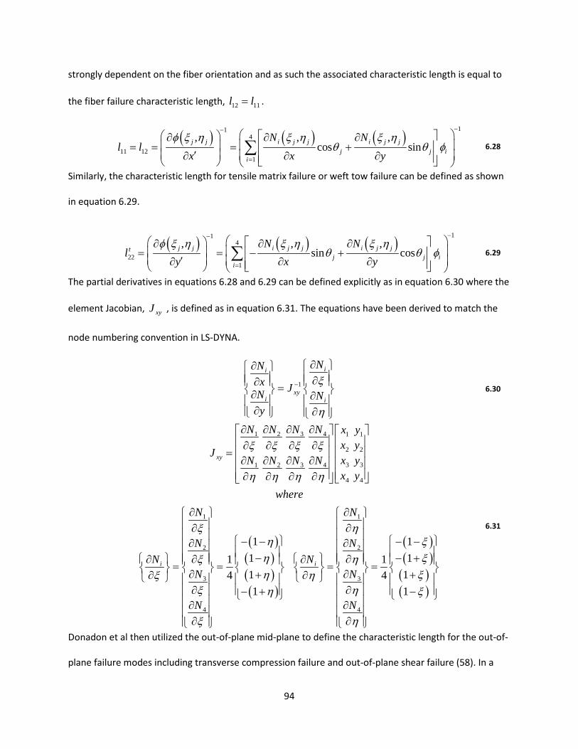
strongly dependent on the fiber orientation and as such the associated characteristic length is equal to
the fiber failure characteristic length, 12 11l l= .
( ) ( ) ( )11
4
11 121
, , ,cos sinj j i j j i j j
j j ii
N Nl l
x x yφ x h x h x h
θ θ φ
−−
=
∂ ∂ ∂ = = = +
′ ∂ ∂ ∂ ∑ 6.28
Similarly, the characteristic length for tensile matrix failure or weft tow failure can be defined as shown
in equation 6.29.
( ) ( ) ( )11
4
221
, , ,sin cosj j i j j i j jt
j j ii
N Nl
y x yφ x h x h x h
θ θ φ
−−
=
∂ ∂ ∂ = = − + ′ ∂ ∂ ∂ ∑ 6.29
The partial derivatives in equations 6.28 and 6.29 can be defined explicitly as in equation 6.30 where the
element Jacobian, xyJ , is defined as in equation 6.31. The equations have been derived to match the
node numbering convention in LS-DYNA.
1
ii
xyi i
NNx JN Ny
x
h
−
∂ ∂ ∂ ∂ = ∂ ∂
∂ ∂
6.30
( )( )( )( )
1 2 3 4 1 1
2 2
3 31 2 3 4
4 4
1 1
2 2
3
4
111141
xy
i i
N N N N x yx y
Jx yN N N Nx y
whereN N
N NN N
N
N
x x x x
h h h h
x hh
hx hhx h
x h
x
∂ ∂ ∂ ∂ ∂ ∂ ∂ ∂ = ∂ ∂ ∂ ∂
∂ ∂ ∂ ∂
∂ ∂ ∂ ∂ − −∂ ∂ − ∂ ∂∂ ∂ = = = ∂ +∂ ∂
∂ − + ∂
∂
( )( )
( )( )
3
4
111
141
N
N
xx
xh x
h
− − − + = ∂ +
∂ − ∂
∂
6.31
Donadon et al then utilized the out-of-plane mid-plane to define the characteristic length for the out-of-
plane failure modes including transverse compression failure and out-of-plane shear failure (58). In a
94

similar fashion, transverse compression characteristic length, 22cl , is defined by equations 6.32, 6.33, and
6.34.
( ) ( ) ( )11
4
221
, , ,cos sinj j i j j i j jc
j j ii
N Nl
x x zφ x ς x ς x ς
θ θ φ
−−
=
∂ ∂ ∂ = = + ′ ∂ ∂ ∂ ∑ 6.32
1
ii
xzi i
NNx J
N Nz
x
ς
−
∂ ∂ ∂ ∂ = ∂ ∂
∂ ∂
6.33
( )( )( )( )
1 2 3 4 1 1
2 2
3 31 2 3 4
4 4
1 1
2 2
3
4
111141
xz
i i
N N N N x zx z
Jx zN N N Nx z
whereN N
N NN N
N
N
x x x x
ς ς ς ς
x ςς
ςx ςςx ς
x ς
x
∂ ∂ ∂ ∂ ∂ ∂ ∂ ∂ = ∂ ∂ ∂ ∂
∂ ∂ ∂ ∂
∂ ∂ ∂ ∂ − −∂ ∂ − ∂ ∂∂ ∂ = = = ∂ +∂ ∂
∂ − + ∂
∂
( )( )
( )( )
3
4
111
141
N
N
xx
xς x
ς
− − − + = ∂ +
∂ − ∂
∂
6.34
For the remaining out-of-plane failure modes, the micro-cracks are assumed to be smeared over
thickness of the ‘brick’ element which corresponds to 90jθ = (58). Thus the characteristic length for
the out-of-plane failure modes is defined as in equation 6.35.
( )1
4
33 13 231
,i j ji
i
Nl l l
zx ς
φ
−
=
∂ = = = ∂ ∑ 6.35
6.5: Erosion Algorithm During ballistic impact simulations, elements can become overly distorted which can lead to
numerical instabilities and premature termination of the simulation. In order to avoid overly distorted
elements, several different techniques can be utilized such as adaptive Lagrangian-Eulerian meshing
95

(ALE) and element erosion. ALE remeshing involves switching from the distorted Lagrangian elements to
an Eulerian definition and back to a Lagrangian defined element mesh. ALE is quite effective in
simulations where large deformations are present however it can add significant computational cost.
Element erosion instead simply maintains the original Lagrangian mesh and deletes elements once given
criteria are met. The downside to erosion algorithms is that the element deletion can lead to unrealistic
mass loss and thus energy imbalances in the presence of large deformations. For the impact velocities in
the present research the deformations are not expected to lead to many distorted elements, thus the
element erosion algorithm will be utilized. Several different criteria can used for the erosion algorithm
such as different combinations of the damage variables, ijd . However it is desired to have criteria that
are not directly involved in the progressive model in order to avoid premature deletion of elements that
could affect the results of the simulation. Yen utilized three simple criteria for the proposed progressive
damage composite model (59) (60). As such, for the present research the same criteria will be utilized.
The first two criteria define the limit compressive and expansive relative element volumes, ECRSH and
EEXPN, as shown in equation 6.36.
el elinitial initial
el el
V VECRSH EEXPNV V
≥ ≤ 6.36
The relative element volume can readily be calculated using the element Jacobian which is simply the
determinant of the deformation gradient, DEFF (61). The deformation gradient is readily obtained by
the material model from the main LS-DYNA program.
( )det DEFelREL initial
el
VV FV
= = 6.37
The remaining criteria is simply a limit on the normal strain, E_LIMT, for the 1-direction for
unidirectional composites and both the 1-/2-directions for plain-weave composites. The aforementioned
criteria were incorporated into the user-defined material model.
96

6.6: Material Model Assumptions And Limitations Throughout the development of the material model several assumptions have been made
regarding the material behavior to simplify either the implementation of the model or the material
behavior itself. These implied assumptions will be explicitly defined and explored at this time. It is well
known that composite materials exhibit a differential in both stiffness and strength when under either
compression or tension. This is due to both the residual stresses from manufacturing processes and the
various mechanisms between the constituents such as adhesion. Although some CDM-based models
such as those for concrete include this differential (62), the present model assumes that there is no
difference in stiffness between compressive and tensile loads. However the model does take into
account the difference in strength through the maximum strain failure criteria for the normal strains.
The failure strains are assumed to be rate-independent based on the experimental data presented in
Tables 6.1 and 6.2 (44). Since strain-based failure criteria are desired, the maximum strain criteria have
been selected as the failure criteria for the present model. Additionally the damage model also takes
into account the strength differential through the characteristic lengths calculated for the 1- and 2-
directions by the smeared crack model. As noted by Zhu et al, from a thermodynamic standpoint the
anisotropic parameters in equation 6.5 of the viscoplastic model would change in accordance with the
loading conditions (63). However establishing and implementing the anisotropic parameter relationships
to the loading condition would lead to an untenable engineering solution. As such the anisotropic
parameters for the viscoplastic model are considered to be constant for all loading conditions. Several
researchers have performed Split Hopkinson Pressure Bar (SPHB) testing to verify whether the
anisotropic parameters could be considered constant for increasing strain rates. Both Thiruppkuzhi et al
and Ninan et al performed off-axis SPHB testing and verified for S2-Glass/8552 epoxy composites that
the anisotropic parameters for the viscoplastic model can be considered constant up to a strain rate of
1000 per second (64) (27). Weeks et al performed SPHB testing to verify the anisotropic parameters for
97

AS4/PEEK composites up to strain rates of 1000 per second (29). Strain rates in excess of 2500 per
second could occur in ballistic impact for the velocity regimes used in previous rounds of experimental
testing (21). Thus for the present research it is necessary to assume that the anisotropic parameters are
constants. Additionally it is assumed that the rate-dependent hardening rule in equation 6.9 can be
extrapolated beyond the range of strain rates used to fit the dual power law. The coupled damage
model divides the material behavior into elastic, plastic, and damage regimes as depicted in Figure 6.6.
Figure 6.6: Material Model Energy Dissipation Due To Elastic, Plastic, And Damage Contributions
The energy dissipation attributed to the elastic, plastic, and damage contributions are EE , PE , and DE ,
respectively. Iannucci et al and Donadon et al considered stress response to be a largely bilinear
response as shown in Figures 6.1 and 6.2 where the damage is due to the elastic and damage
contributions. Based on the bilinear response assumption, Iannucci et al approximated the area
underneath the curve or the energy dissipation to be simply the area of a triangle as evidenced in
equations 6.18 and 6.19. In order to simplify the implementation of the material model, the same
bilinear response will be assumed. This saves computational effort by avoiding explicitly integrating the
stress-strain relationship to determine the energy balance. It is assumed that there will be negligible
98

error introduced in the energy balance for the damage model by the bilinear response assumption.
Currently the material model is only derived for explicit solver FEM codes since they are more efficient
for the anticipated strain rate regimes present in ballistic impact. The model could be readily
implemented into implicit FEM solvers since the return mapping algorithm is unconditionally stable and
also maintains the quadratic rate of convergence for the Newmark implicit integration (38). This would
allow for use of the model in long duration quasi-static simulations. Derivation of the consistent tangent
modulus tensor is necessary for the stiffness matrix calculations present in the implicit integration
scheme.
6.7: LS-DYNA Implementation The coupled viscoplastic progressive damage material model has been implemented into LS-
DYNA as a user-defined material model. LS-DYNA allows for the user-defined material model (UMAT)
through programming a Fortran subroutine which can be called using the user-defined material model
interface (65). The LS-DYNA Fortran source code for the user defined interface is written using Fortran
77, 90, and 95 conventions. The UMAT can be written in either scalar or vectorized subroutines. The
vectorized subroutines group the models’ elements into blocks of up to 192 elements. Vectorized
subroutines offer an efficiency advantage over scalar subroutines since fewer calls are made to the
material subroutine during each time step (65). For the present research a vectorized UMAT will be
implemented on the Auburn University High Performance Compute Cluster (AU HPCC) in order to
exploit the computational power. The AU HPCC utilizes the MPICH Message Passing Interface running
Redhat Linux on 512 processors over 4 nodes (66). LS-DYNA can utilize either Shared Memory Processing
(SMP) or Massively Parallel Processing (MPP) for single and multiple processor computations (65). The
UMAT was implemented in both SMP and MPP double precision versions of LS-DYNA release 7.0. For the
cluster configuration and release of LS-DYNA, the Intel Fortran Compiler version 10.1 is required.
99

6.7.1 : LS-DYNA UMAT Overview The overview of the coupled viscoplastic damage model algorithm is outlined in the flowchart in
Figure 6.7. Before the simulation begins, LS-DYNA initializes the Cauchy stresses and history variables for
each element. During the pre- simulation initialization the equivalent plastic strain and plastic strain rate
also need to be defined to remain consistent with the dual power law. A result of using a power law is
that upon loading the equivalent plastic strain and plastic strain rate will instantaneously progress (22).
Based on the precision for the history variables, the equivalent plastic strain and plastic strain rate are
both initialized to a value of 1.0 16E − . During the simulation, for each load cycle, LS-DYNA calls the
UMAT and passes Cauchy stresses and the incremental strains in addition to the history variables which
includes the equivalent stress, equivalent plastic strain and plastic strain rate, plastic strains, damage
variables, and maximum strain from the previous time step for each element. The characteristic lengths
are calculated using relations defined in the 3-D smeared crack model for the element. Next, the
viscoplastic return mapping algorithm calculates the effective stresses, plastic strains and equivalent
plastic strain and plastic strain rate using the present state of strain. The progressive damage model
then calculates the current value for the damage variables. Using the damage variables, the Cauchy
stresses can be calculated from the effective stresses. The values for the Cauchy stresses and the history
variables are returned to the main LS-DYNA executable for use in the next time step calculations.
100

Figure 6.7: Coupled Viscoplastic Damage Material Model Flowchart
6.7.2 : Smeared Crack Model Algorithm The smeared crack model algorithm is depicted in the flowchart shown in Figure 6.8. As with
most finite element codes LS-DYNA renumbers the nodes and elements during the simulation to
improve calculation efficiency. The node and element numbering used in the time step calculations are
referred to as the internal ID while the numbering defined in the LS-DYNA model is the external ID. For
each element during the current time step, the UMAT requests the external ID for the element. Then
using the external element ID, the internal node IDs are obtained. LS-DYNA provides the internal node
101

IDs in the same order as defined in Figure 6.4 which is critical to ensure that a positive element Jacobian
is obtained. Otherwise the simulation will terminate prematurely due to a negative element volume.
Next the algorithm uses the internal node IDs to obtain the global x-y-z coordinates for the elements’
nodes. For both the in-plane and out-of-plane virtual planes, as defined in Figures 6.4 and 6.5,
associated with in-plane and out-of-plane failure modes, the global coordinates are calculated. The Q4
virtual nodes are calculated using the midpoint rule for the hexahedral element node pairs as defined in
Table 6.3. The node associations defined in Table 6.3 are easily verified by Figures 6.4 and 6.5.
Table 6.3: Virtual Mid-plane Q4 Element Node-Hexahedral Element Node Pair Associations
Using the calculated global coordinates for the virtual mid-planes, equations 6.30, 6.31, 6.33, and 6.34
are used to calculate the partial derivatives of the virtual Q4 mid-plane element isoparametric functions
with respect to the global coordinates.
{ } { }0 0 0cos ,sin ,0T
f f fθ θ=e 6.38
{ } { }
{ }0
0
DEFf
f DEFf
F
F
=
ee
e 6.39
( )( )
1 2tan
1f
ff
θ −
=
ee
6.40
Since it is anticipated that a significant amount of element deformation may occur during the
simulation, the element deformation gradient, DEFF , is used to calculate the current fiber angle, fθ .
LS-DYNA allows the UMAT to request the deformation gradient, DEFF , from the main program. The
Node 1 Node 21 1 52 2 63 3 74 4 81 1 42 2 33 6 74 5 8
In-Plane
Out-of-Plane
Hexahedral Element Node PairQ4 Node ID
Virtual Midplane
102

deformation gradient is passed into the material model subroutine at the end of the history variable
array. The initial fiber direction vector, 0fe , is defined in equation 6.38. The current fiber direction can
then be calculated using the deformation gradient as defined in 6.39. The current fiber direction is then
calculated using the inverse tangent of the x and y components of the fiber direction vector as defined
in equation 6.40. Given the current state of strain, the current fiber angle and the relations defined in
equations 6.28, 6.29, 6.32, and 6.35 are used to calculate the characteristic lengths for the element.
Figure 6.8: Smeared Crack Model Algorithm Flowchart
6.7.3 : Viscoplastic Return Mapping Algorithm The viscoplastic damage model is coupled through the integration algorithm. The approach
presented by Chen et al (49) will be utilized since it provides a simpler method than the thermodynamic
framework of Zhu et al (63) to fully couple the viscoplastic and damage models. Since the material
103

model will be only implemented for the explicit solver, the consistent tangent stiffness matrix does not
need to be defined. Additionally since explicit solvers do not have the convergence issues due to strain
softening and damage progression as implicit solvers, viscous regularization is not necessary for the
present research.
As is typical for most finite element codes, LS-DYNA is based on an incremental strain driven
solution. For each load cycle, the incremental strains, time increment, state variables, and stress state
from the previous load step, n, are passed to the material model which returns the updated state
variables and stress state for the current load step, n+1, for each element. Since the material model is
intended for highly dynamic simulations where large strain increments can occur in a load cycle, the
integration algorithm for viscoplastic model should be stable for all loading conditions. For the present
research a return mapping algorithm will be utilized since it is unconditionally stable and reasonably
efficient.
Return mapping algorithms transform the nonlinear problem from a system of ordinary
differential equations into an algebraic constrained optimization problem (38). The algorithms are based
on the split operator methodology which divides the material response into the elastic and plastic
contributions (38) (39). Typically the response is decomposed into an elastic predictor and plastic
corrector where the response is returned to the plastic yield surface. The integration scheme usually for
the return mapping algorithms is either fully implicit or semi-implicit. Fully implicit integration schemes
are desired where unconditional stability is required. Wang et al (42) proposed a fully implicit backward
Euler return mapping algorithm that is applicable to the yield function presented in equation 6.10. The
Wang return mapping algorithm was referred to as the ‘Consistency Model’ since the integration is
constrained by the consistency condition. The consistency condition, equation 6.42, results from the
Kuhn Tucker or loading/unloading conditions, equation 6.41.
104

0, 0, 0 ( , , ) 0F F where Fλ λ σ λ λ≥ ≤ ≤ = 6.41
( , , ) : 0F F FF σ λ λ σ λ λ
σ λ λ∂ ∂ ∂
= + + =∂ ∂ ∂
6.42
( )
( )
1 1
1 1
, 0 , 0 0 0 , 0 , 01 1 1 1
2,
2
, , 0;
0 , ,
En tr n n
p ptr n n
p k p k p k k p k p kn n n tr tr n n
th
k E p k
Calculate Elastic PredictorC
if F plastic state
Initialize
F F
Begin k iteration
FH S
ε σ σ ε
σ ε ε
ε ε ε σ σ σ ε ε
εσ
+ +
+ +
= = = = = =+ + + +
∆ = + ∆
≥
∆ = = = =
∂= + ∆ ∂
1
2 , 2,
, 1 ,
1 , 11 1
, 11 , 1
1
1
, ,
,
T p kk k p k
p pp p
kp k p k
k
k E p kn n n
p kk p p k
tr n
k
F F F F F FHt t
F
FC
F Ft
if F tol perform n
εβ εσ σ σ ε εσ ε λε
ε εβ
σ σ ε εσ
εσ ε ε
−
+
+ ++ +
++ +
+
∂ ∂ ∂ ∆ ∂ ∂ ∂ = + ∆ + − − ∂ ∂ ∂ ∂ ∆ ∂ ∆∂ ∂ ∂
∆ = ∆ +
∂ = + ∆ − ∆ ∂ ∆
= + ∆ ∆ >
1; n tr
ext iterationelse elastic state σ σ+ =
Figure 6.9: Viscoplastic Return Mapping Algorithm
Simplifying the general form presented by Wang et al, the return mapping algorithm can be
summarized as in Figure 6.9. The partial derivatives for the plastic yield function defined by equation
6.10 are defined in equations 6.43 - 6.45. For each time step, t∆ , the algorithm begins with the elastic
predictor step to calculate the trial stresses, trσ , from the strain increments, 1nε +∆ , using the elastic
stiffness matrix, EC . During the elastic predictor step plasticity is ‘frozen’ where the equivalent plastic
105

strain is zero, , 01 0p k
nε =+∆ = . If the material state predicted exceeds the yield surface, the material state is
returned iteratively until yield function is within a predefined error tolerance.
( ) ( )
1 1
1n n
p p
m mp p p pp p
F F mn n
ε εε ε ε εχ ε χ ε
∂ ∂ = − = ∂ ∂
6.43
{ }
( )( )
( )
212 31 31 11 12 12 22 31 31 33 66 12
212 12 22 23 12 12 22 23 23 33 44 23
231 31 11 23 23 22 31 23 23 33 55 13
32
2
2
2
TF A B C D E F
where
A D a
B E a
C F a
σ σ
α σ α σ α σ σ
α σ α σ α σ σ
α σ α σ α σ σ
∂=
∂
= Α + Α − Α − Α =
= −Α + Α + Α − Α =
= −Α − Α + Α + Α =
6.44
106

2 2 2 2 2 2
21 2 1 3 1 12 1 23 1 13 1
2 2 2 2 2 2
22 1 2 3 2 12 2 23 2 13 22 2 2 2 2 2
2 23 1 3 2 3 12 3 23 3 13 32 2 22
12 1 12 2 12
F F F F F F
F F F F F F
F F F F F FF
F F F
σ σ σ σ σ σ σ σ σ σ σ
σ σ σ σ σ σ σ σ σ σ σ
σ σ σ σ σ σ σ σ σ σ σσ
σ σ σ σ σ
∂ ∂ ∂ ∂ ∂ ∂∂ ∂ ∂ ∂ ∂ ∂ ∂ ∂ ∂ ∂ ∂∂ ∂ ∂ ∂ ∂ ∂
∂ ∂ ∂ ∂ ∂ ∂ ∂ ∂ ∂ ∂ ∂∂ ∂ ∂ ∂ ∂ ∂
∂ ∂ ∂ ∂ ∂ ∂ ∂ ∂ ∂ ∂ ∂ ∂=∂ ∂ ∂∂
∂ ∂ ∂ ∂ ∂ ∂
2 2 2
23 12 23 12 13 12
2 2 2 2 2 2
223 1 23 2 23 3 23 12 23 13 232 2 2 2 2 2
213 1 13 2 13 3 13 12 13 23 13
2
21
3
F F F
F F F F F F
F F F F F F
where
F
σ σ σ σ σ σ
σ σ σ σ σ σ σ σ σ σ σ
σ σ σ σ σ σ σ σ σ σ σ
σ
∂ ∂ ∂
∂ ∂ ∂ ∂ ∂ ∂ ∂ ∂ ∂ ∂ ∂ ∂ ∂ ∂ ∂ ∂ ∂ ∂ ∂ ∂ ∂ ∂
∂ ∂ ∂ ∂ ∂ ∂ ∂ ∂ ∂ ∂ ∂ ∂ ∂ ∂ ∂ ∂ ∂
∂=
∂( )
22
12 31 31 12 122 21 2 1 2
2 2
31 312 23 1 3 12 1 122 2
2 223 1 23 13 1 13
2
2
32 2
3 32 2
3 32 2
F F FA A
F F F FA A
F F F FA A
F
α σ α σσ σ σ σ σ σ
α σσ σ σ σ σ σ σ σ
σ σ σ σ σ σ σ σ
σ
∂ ∂ ∂Α + Α − = −Α − ∂ ∂ ∂ ∂ ∂ ∂ ∂ ∂
= −Α − = − ∂ ∂ ∂ ∂ ∂ ∂ ∂ ∂ ∂ ∂
= − = − ∂ ∂ ∂ ∂ ∂ ∂ ∂∂
( )
( )
22
23 12 12 23 232 2 22 3 2 2
2 2
2 212 2 12 23 2 232 2
231 23 232 2 2
13 2 13 3 3
3 32 2
3 32 2
3 32 2
F F FB B
F F F FB B
F F F FB C
α σ α σσ σ σ σ σ σ
σ σ σ σ σ σ σ σ
α σσ σ σ σ σ σ σ
∂ ∂ ∂= Α + Α − = −Α − ∂ ∂ ∂ ∂
∂ ∂ ∂ ∂= − = − ∂ ∂ ∂ ∂ ∂ ∂
∂ ∂ ∂ ∂= − = Α + Α − ∂ ∂ ∂ ∂ ∂
∂
2 2
2 212 3 12 23 3 232 2
66 122 2 213 3 13 12 12
2 2
2 223 12 23 13 12 13
2
23
3 32 2
3 3 22 2
3 32 2
F F F FC C
F F F FC a
F F F FD D
F
σ σ σ σ σ σ σ σ
σ σσ σ σ σ σ σ σ
σ σ σ σ σ σ σ σ
σ
∂ ∂ ∂= − = − ∂ ∂ ∂ ∂ ∂ ∂
∂ ∂ ∂ ∂= − = − ∂ ∂ ∂ ∂ ∂
∂ ∂ ∂ ∂= − = − ∂ ∂ ∂ ∂ ∂ ∂
∂∂
2
44 232 2 223 13 23 13
2
55 132 213 13
3 322 2
3 22
F F Fa E
F Fa
σ σσ σ σ σ σ σ
σ σσ σ σ
∂ ∂ ∂= − = − ∂ ∂ ∂ ∂
∂ ∂= − ∂ ∂
6.45
107

6.7.4 : Damage Model Algorithm The overall damage model algorithm is summarized in Figure 6.10. As established in Section 6.3,
the maximum strain failure criteria will be used to determine damage initiation. In addition, different
failure strains will be defined for the normal strains when the material is under either compressive or
tensile loading. As such a total of nine damage variables will be tracked through the load time history:
11 11 22 22 33 33 12 23 13, , , , , , , ,t c t c t cd d d d d d d d d . There are nine maximum strains, maxε , associated with each of
the damage variables.
Figure 6.10: Damage Model Algorithm Flowchart
The damage progression for the normal strains is dependent on the current state of strain. The
corresponding failure strain is selected and used to determine if failure has occurred. If failure is
detected by the maximum strain criteria, damage has either initiated or progressed. At the time of
damage initiation, maxε is calculated using equation 6.20. In order to maintain the initial energy balance
illustrated in Figure 6.1, the value of maxε at damage initiation is stored as a history variable and used in
the subsequent time steps to calculate the progression of damage. If full damage has not occurred yet,
1niid < , then the damage for the current time step, 1n
iid + , is calculated using equation 6.23. Since
damage is an irreversible process, damage may only progress in an increasing fashion. As such the
108

calculated damage value for the current time step, 1niid + , is compared to the previous time step value,
niid , and if the value has not increased, the previous value is stored to preserve the damage accrued. The
resulting damage variable from the above algorithm is then stored as a history variable and returned to
the main LS-DYNA program. A summary of the damage progression logic for the normal strains is
outlined in Figure 6.11.
( )
( )max
,
, 1
, 1 ,
, 1 ,
0 ( )
1
( Pr )
variable
iit
ii fail ii
t
iit nii
t nii
t n t nii iit n t nii ii
tii
if then Tensile Strain
if then
if Damage Initiated then
Calculate
if d thenCalculate d
if d d then Ensure Damage ogressiond d
Update d historyel
ε
ε ε
ε
+
+
+
≥
≥
<
<
=
( )
( )max
c,
c, 1
c, 1 c,
c, 1 c,
( )
1
( Pr )
variable
c
ii fail ii
c
iin
iin
iin n
ii iin n
ii iicii
se Comressive Strain
if then
if Damage Initiated then
Calculate
if d thenCalculate d
if d d then Ensure Damage ogressiond d
Update d history
ε ε
ε
+
+
+
≥
<
<
=
Figure 6.11: Normal Strain Damage Progression Algorithm
The damage progression of the shear strains follows the same general logic as the normal strains. The
algorithm is illustrated in Figure 6.12.
109

( )
( )max
1
1
1
0
1
( Pr )
variable
ij
ij fail ij
ij
nij
nij
n nij ij
n nij ij
ij
if then
if then
if Damage Initiated then
Calculate
if d then
Calculate d
if d d then Ensure Damage ogression
d d
Update d history
ε
ε ε
ε
+
+
+
≥
≥
<
<
=
Figure 6.12: Shear Strain Damage Progression Algorithm
After the effective stresses are calculated for the current time step using the viscoplastic return mapping
integration scheme, is used to calculate the nominal Cauchy stresses with the relationship described by
equation 6.2.
6.7.5 : Erosion Criteria Algorithm LS-DYNA allows user-defined material models to access the erosion algorithm utilized by other
material models natively implemented into the program. The erosion algorithm simply removes an
element and its’ mass from the simulation solution as a means to prevent severe element distortion.
The UMAT must define the criteria for which determine when the erosion algorithm is called. A logical
array, FAILELS, is passed between the main LS-DYNA program and the UMAT which maintains which
elements have failed and been eroded or deleted from the simulation. The outline of the calculation of
the erosion criteria is depicted in Figure 6.13.
110

( )
11
11 22
det
_
_ _
DEFelREL initial
el
REL REL
VCalculate V FV
if V EEXPN OR V ECRSH thenFAILELS TRUE
if Unidirectional thenif E LIMT then
FAILELS TRUEelseif Plain Weave then
if E LIMT OR E LIMT thenFAILELS TRUE
if FAILELS TRUE the
ε
ε ε
= =
≥ ≤=
≥
=
≥ ≥
==
0ij
nσ =
Figure 6.13: Erosion Criteria Algorithm
Using the erosion criteria from Yen highlighted in Section 6.5, ECRSH, EEXPN, and E_LIMT, the
element failure can easily be determined. The relative element volume is calculated from the
determinant of the deformation gradient. Next the relative element volume is compared to both the
EEXPN and ECRSH criteria and the element is failed if the criteria are met. Depending on whether the
composite panel considered is unidirectional or plain weave, either the absolute value of the total strain
in the 1-direction or both the 1- and 2-directions are compared to the E_LIMT criteria. Finally if the
element has failed, the Cauchy stresses can be set to zero.
6.8: LS-DYNA UMAT Model Validation In order to validate the material model, published experimental data for IM7/8552
unidirectional composite was considered for several single element and coupon test cases. The simple
test cases include the viscoplastic behavior under off-axis uniaxial tensile loading, mesh sensitivity for
energy dissipation, and damage progression to cyclic loading.
111

6.8.1 : IM7/8552 Material Model Parameters As mentioned previously, Koerber et al performed both quasi-static and SPHB off-axis
compression testing for IM7/8552 unidirectional composites (44) (51). The off-axis loading was
performed from 0° to 90° with increments of 15°. The quasi-static cases were performed on a hydraulic
mechanical tester at a constant strain rate of 4.0E-4 per second. The SPHB strain rates ranged from ~100
to 400 per second depending on the off-axis angle. The IM7/8552 composite exhibited significant
nonlinear behavior at the larger off-axis angles where the material behavior is matrix-dominated. At the
shallower angles where the behavior is fiber-dominated the response is largely linear elastic. This
behavior is expected due to the fact that carbon fiber has been reported to be rate-independent, linear
elastic such as the case of T300 reported by Zhou et al (67). Also evident is that the IM7/8552 composite
at larger off-axis angles is significantly rate-dependent in that the composite becomes stiffer at higher
loading rates.
The elastic constants were either reported values (51) (68), calculated, or estimated under the
assumption of transverse isotropy. The thermodynamic constraints presented by Jones were observed
for the elastic constant estimations (69). The material constants are summarized in Table 6.4. LS-DYNA
requires the density, elastic modulus, and bulk modulus be defined for time step, boundary condition,
and contact calculations (65). It was observed during the research that for orthotropic models the
simulation stability was highly dependent on the elastic and bulk moduli defined. A poor definition of
the moduli caused negative element volume errors similar to the issue present in the simulation of soft
materials such as foam (70). As such the moduli were increased to the maximum values calculated
within 1-/2-plane with a rotation about the 3-axis. The exaggerated moduli values improved the element
stability to varied loading conditions while having no effect on the stress response in the simulation.
112

Table 6.4: IM7/8552 Material Constants
From the optimization algorithm outlined in Sections 5.5 and 5.6 the anisotropic and hardening
rule parameters can be determined. Using the relations in equations 5.8 and 5.9 with the results for the
1-D off-axis loading case considered by the optimization algorithm, the anisotropic parameters for the
3D UMAT can be expressed as shown in Table 6.5.
Table 6.5: IM7/8552 Anisotropic Parameters
The hardening rule parameters calculated by the optimization algorithm are reiterated in Table 6.6.
Table 6.6: IM7/8552 Hardening Rule Parameters
The fracture energies utilized for the IM7/8552 composite were obtained from data presented by
Camanho et al summarized in Table 6.7 (45). The fracture energies are related to intralaminar and
interlaminar crack growth under Mode I and Mode II fracture.
Type Constant Value SourceDensity (ton/mm3) ρ 1.59E-09 Koerber
Modulus (GPa) E 158.720 CalculatedBulk Modulus (GPa) K 64.931 Calculated
E1 171.420 ASTM 3039E2 9.080 ASTM 3039E3 9.080 EstimatedG12 5.068 CalculatedG23 3.492 CalculatedG13 5.068 Calculatedv12 0.32 ASTM 3039v23 0.30 Estimatedv13 0.32 Estimated
Moduli (GPa)
Poisson Ratios
A12 A23 A31 a44 a55 a66 α12 α23 α31
0.1 0.1 11.0174 2.0 48.0 48.0 10.4964 1.0000 0.0953
A, (MPa)-n n χ, (MPa)-n m4.9756E-17 4.3930861 1.0010E-17 -0.16103
113
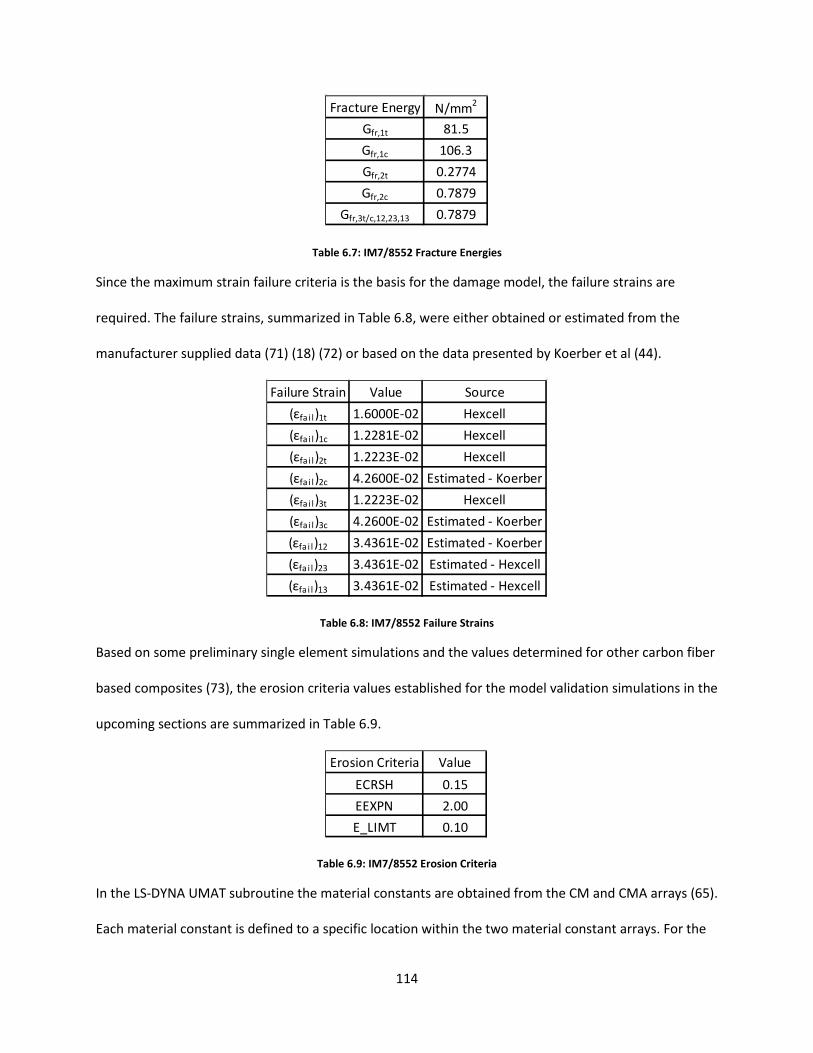
Table 6.7: IM7/8552 Fracture Energies
Since the maximum strain failure criteria is the basis for the damage model, the failure strains are
required. The failure strains, summarized in Table 6.8, were either obtained or estimated from the
manufacturer supplied data (71) (18) (72) or based on the data presented by Koerber et al (44).
Table 6.8: IM7/8552 Failure Strains
Based on some preliminary single element simulations and the values determined for other carbon fiber
based composites (73), the erosion criteria values established for the model validation simulations in the
upcoming sections are summarized in Table 6.9.
Table 6.9: IM7/8552 Erosion Criteria
In the LS-DYNA UMAT subroutine the material constants are obtained from the CM and CMA arrays (65).
Each material constant is defined to a specific location within the two material constant arrays. For the
Fracture Energy N/mm2
Gfr,1t 81.5Gfr,1c 106.3Gfr,2t 0.2774Gfr,2c 0.7879
Gfr,3t/c,12,23,13 0.7879
Failure Strain Value Source(εfa i l)1t 1.6000E-02 Hexcell(εfa i l)1c 1.2281E-02 Hexcell(εfa i l)2t 1.2223E-02 Hexcell(εfa i l)2c 4.2600E-02 Estimated - Koerber(εfa i l)3t 1.2223E-02 Hexcell(εfa i l)3c 4.2600E-02 Estimated - Koerber(εfa i l)12 3.4361E-02 Estimated - Koerber(εfa i l)23 3.4361E-02 Estimated - Hexcell(εfa i l)13 3.4361E-02 Estimated - Hexcell
Erosion Criteria ValueECRSH 0.15EEXPN 2.00E_LIMT 0.10
114

current implementation the populated material keycard is shown in Figure 6.14. The anisotropic
parameters 12α , 23α , and 31α can be calculated by the UMAT as shown in Figure 6.14 by leaving the
values entered as zero or can also be overridden, if necessary, by explicitly entering values. This allows
the analyst more flexibility in defining anisotropic plastic behavior mentioned previously. For the
following simulations an error tolerance, ERRTOL, of 1.0E-3 is used for the viscoplastic return mapping
algorithm. As noted in Figure 6.14, the consistent system of units are metric ton, millimeter, and
seconds such that the derived units for force, pressure, and energy are newtons, megapascals, and
kilojoules per squared millimeter, respectively.
Figure 6.14: Populated LS-DYNA Keycard For Coupled Viscoplastic Damage UMAT
In addition to the material parameters, LS-DYNA requires the material density, and the bulk and
shear moduli for the critical time step calculation. Additionally the material orientation must be defined
for orthotropic material models. The parameter selection IORTHO = 1 denotes the directional
115

behavior of the model and therefore definition of the material orientation is required. For the present
work due to the geometry and layup pattern in the simulations, the material orientations were defined
with respect to the global coordinate system, AOPT = 2 , through definition of the vectors A and D
where the parameters 1 2 3a , a , a and 1 2 3d , d , d are the respective x, y, and z vector components. As
noted previously the routine has been implemented in the vectorized form which is noted by
IVECT = 1 . Since the element erosion algorithm will be utilized, the parameter IFAIL is set to one.
The deformation gradient is requested from the main routine by setting IHYPER = 1 . The LS-DYNA
main program provides the deformation gradient to the material model through the history variables.
For the present implementation of the material model, forty four history variables are used by the
routine and are requested by the parameter NHV . Currently no equation of state is implemented and
thus the equation of state parameter, IEOS , is set to zero.
6.8.2 : LS-DYNA User Defined Material Implementation Validation In order to verify that the Fortran subroutine is performing as intended, a series of single
element simulations were performed to evaluate the viscoplastic model using the IM7/8552 data
presented in previous sections. In order to isolate the viscoplastic model behavior, the simulations were
performed without the evaluation of damage. Damage will also be considered in the upcoming section.
Off-axis uniaxial tension was performed on a unit sized element for rotations about the Z- and X-axes as
shown below in Figure 6.15 where the X-axis if the fiber direction as defined previously. Off-axis uniaxial
tension load case was selected since it will demonstrate the nonlinear model behavior in various
directions and the simulation results can be readily verified using the 1-D simplification of the load case
with the 1-D return mapping integration scheme summarized in Figure 5.3. It should be noted that
although the 1-D return mapping algorithm presented in Figure 5.3 has been derived explicitly for off-
axis uniaxial tension/compression loading with a rotation about the Z-axis, a similar simplification can be
easily obtained for rotations about the X-axis. The 1-D return mapping algorithms to solve the off-axis
116

load cases have been programmed into MATLAB in order to compare the results calculated by the LS-
DYNA implementation.
Figure 6.15: Off-Axis Tension Rotation About (a) Z-Axis (b) X-Axis
Rotation angles of 0°, 30°, 60°, and 90° about both the Z- and X- axes were simulated at an
arbitrary constant strain rate of 100 per second. Tension at a constant strain rate was enforced through
displacement at the element boundary as shown in Figure 6.16. The off-axis angles were defined
through specification of the material orientation with respect to the global coordinate system. LS-DYNA
internally performs the coordinate system transformations to obtain the correct material response. Due
to the directional behavior of the model and to reduce the error due to element rotations, the
*CONTROL_ACCURACY keyword was selected so that the second order terms will be utilized in the
stress updates (65).
117

Figure 6.16: LS-DYNA Single Element Off-Axis Tension Boundary Conditions and Material Orientations for Rotations About: a) Z-Axis b) X-Axis
Figures 6.17, 6.18, 6.19, and 6.20 below compare the 1-D model calculations to the 3-D LS-DYNA
user defined material subroutine output for the Z-axis off-axis cases. As can be seen from the plots, the
simulation results match almost identically to the calculated 1-D simplification calculations. However the
30° case shows some difference at the larger strains. Most of the discrepancy in the results is due to
element rotation that is present at higher strains in the simulations. As the element rotates the off-axis
loading angle is affected. The reason for the element rotation is the highly directional behavior of the
material considered. For the 30° load case the material behavior is largely fiber-dominated and in
combination with the off-axis strain state which consists of normal and shear strains, the element has a
tendency to rotate due to the shear contributions. IN order to reduce or eliminate the element rotation,
additional nodal constraints would be necessary. However for the purposes of validating the LS-DYNA
implementation, it is desired to have a minimal amount of nodal constraints in order to avoid over
constraining the element and affecting the LS-DYNA calculations. Thus the minimal boundary constraints
were only utilized.
118

Figure 6.17: LS-DYNA Comparison; Off-Axis Tension 0° Rotation About Z-Axis
Figure 6.18: LS-DYNA Comparison; Off-Axis Tension 30° Rotation About Z-Axis
119

Figure 6.19: LS-DYNA Comparison; Off-Axis Tension 60° Rotation About Z-Axis
Figure 6.20: LS-DYNA Comparison; Off-Axis Tension 90° Rotation About Z-Axis
120

Figures 6.21, 6.22, 6.23, and 6.24 compare the 1-D calculations for the off-axis tensile load cases
with a rotation about the X-axis. For all the angles considered, the results are nearly identical to the
expected response calculated in MATLAB. Additionally, since the IM7/8552 unidirectional composite for
the present case is considered to be transversely isotropic, the angles of 0° and 90°, and 30° and 60° are
identical as well.
Figure 6.21: LS-DYNA Comparison; Off-Axis Tension 0° Rotation About X-Axis
121
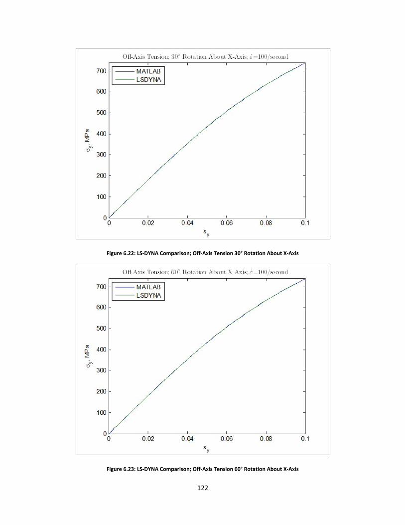
Figure 6.22: LS-DYNA Comparison; Off-Axis Tension 30° Rotation About X-Axis
Figure 6.23: LS-DYNA Comparison; Off-Axis Tension 60° Rotation About X-Axis
122
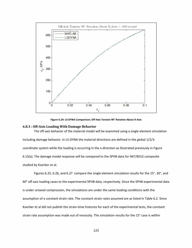
Figure 6.24: LS-DYNA Comparison; Off-Axis Tension 90° Rotation About X-Axis
6.8.3 : Off-Axis Loading With Damage Behavior The off-axis behavior of the material model will be examined using a single element simulation
including damage behavior. In LS-DYNA the material directions are defined in the global 1/2/3-
coordinate system while the loading is occurring in the x-direction as illustrated previously in Figure
6.15(a). The damage model response will be compared to the SPHB data for IM7/8552 composite
studied by Koerber et al.
Figures 6.25, 6.26, and 6.27 compare the single element simulation results for the 15°, 30°, and
60° off-axis loading cases to the experimental SPHB data, respectively. Since the SPHB experimental data
is under uniaxial compression, the simulations are under the same loading conditions with the
assumption of a constant strain rate. The constant strain rates assumed are as listed in Table 6.2. Since
Koerber et al did not publish the strain-time histories for each of the experimental tests, the constant
strain rate assumption was made out of necessity. The simulation results for the 15° case is within
123

reasonable agreement with the experimental data in the failure strain. From Figure 6.25, large
oscillations in the stress response are observed post-damage. These oscillations are due to the explicit
solver and the damage model. In order to avoid the oscillating behavior, global damping could be added
to the simulation without affecting the material stress response.
Figure 6.25: 15° Off-Axis Compressive Loading With Damage Model; Strain Rate 122 1/sec
The 30° case comparison presented in Figure 6.26 shows that the model does not predict the ultimate
strain well. For the loading case the damage variable 12d is leading to the premature damage. Although
the shear failure strain ( )12failε has been increased beyond what has been reported by the
manufacturer of the composite, the maximum failure strain criteria does not predict the ultimate strain
for the 30° case well.
124

Figure 6.26: 30° Off-Axis Compressive Loading With Damage Model; Strain Rate 246 1/sec
Figure 6.27: 60° Off-Axis Compressive Loading With Damage Model; Strain Rate 367 1/sec
Considering the 60° case in Figure 6.27, the model shows a discrepancy between the failure strain
obtained experimentally. The model discrepancies between the predicted and the observed failure
strains result from the underlying assumptions where the failure strains remain constant regardless of
the strain rate and that all of the behavior pre-failure is plastic. However in reality the plastic and
damage processes occur concurrently. As such in experimental testing the reported failure strains are at
the onset of damage. The failure strains used in the simulations, Table 6.8, likely do not include all of the
plasticity and damage. Despite this deficiency the model should still be suitable since the intended
ballistic simulation uses a ( )7
0 90 0
layup (74).
125

6.8.4 : Cyclic Loading As damage accumulates the stiffness of the composite progressively degrades accordingly. This
is also a physically based behavior present in cyclic loading of composite materials in experimental
testing. As a means to demonstrate the progressive nature of the damage model, a cyclic tensile loading
simulation was created. A single element simulation was used where the loading direction is aligned
with 1-axis material direction along the fiber axis. The strain rate was held constant at 1 per second. For
the simulation the element remained under tension and was cyclically loaded and unloaded until the
element was fully damaged. Figure 6.28 demonstrates the progressive nature of the damage model.
From the figure it is apparent that the modulus is progressively degrading. In addition plastic strain is
accumulating as the damage progresses.
Figure 6.28: Progressive Damage Of Uniaxial Tensile Cyclic Loading Case
6.8.5 : Mesh Sensitivity Study One of the key considerations of the material model is the damage model and the ability to
dissipate energy due to fracture regardless of the specific mesh discretization. Similar to Oliver and
Donadon et al, a coupon test comparison using solid hexahedral elements was performed at a strain
rate of 1 per second with the dimensions of 10 x 5 x 1 mm (length, width, and depth) (53) (58). The
126

coupons are under uniaxial tension along the length axis. The boundary conditions for the coupons are
illustrated in Figure 6.29 where one side is fixed such that contraction due to Poisson effect can still
occur and the other side is under constant displacement to approximate constant strain rate.
Figure 6.29: Mesh Sensitivity Coupon Boundary Conditions
The five coupons considered have different levels of mesh density and element distortion as shown in
Figure 6.30.
Figure 6.30: Mesh Sensitivity Coupon Comparison
127

The force exerted on the coupon and the resulting displacement for all of the coupons
considered is summarized in Figure 6.31 where the area underneath the curve represents the energy
dissipated by the coupon. From the figure it is apparent that the material model is largely mesh
insensitive for the coupons considered. However there is still some variation present in the energy
dissipated. This is largely due to the location of damage and its proximity to either the fixed or
displacement boundary condition. As noted by Donadon et al, the damage location results from the
rounding errors for the viscosity used to average the stress wave over the elements (58). Coupons 1, 4,
and 5 have the greater level of damage at the fixed boundary condition while Coupons 2 and 3 occur on
the constant displacement boundary condition. These results are corroborated by the disparity in the
energy dissipated between the two Coupon groups shown in Figure 6.31.
Figure 6.31: Fracture Energy Dissipation Comparison
In order to establish the rate of convergence with mesh refinement, the structured or mapped meshes
of Coupons 1, 2, and 3 are compared with maximum force prior to full damage. Figure 6.32 shows that
the smeared crack model allows for the solution to converge rapidly as the element number is increased
from 8 to 200 for Coupons 1 and 3, respectively.
128

Figure 6.32: Smeared Crack Model Mesh Convergence; Maximum Force vs Element Number
Contour plots of the coupons at the time where one of the elements has reached full damage are
provided in Figures 6.33 through 6.37 to show the location of maximum damage in the coupon.
Figure 6.33: Mesh Sensitivity Damage Study Coupon 1
129

Figure 6.34: Mesh Sensitivity Damage Study Coupon 2
Figure 6.35: Mesh Sensitivity Damage Study Coupon 3
130

Figure 6.36: Mesh Sensitivity Damage Study Coupon 4
Figure 6.37: Mesh Sensitivity Damage Study Coupon 5
131

Chapter 7 : IM7/8552 Ballistic Impact Simulation Results The material model response to ballistic impact will be considered using the same IM7/8552
unidirectional composite presented previously. Karthikeyan et al performed experimental testing
comparing the ballistic response of IM7/8552 and Ultra High Molecular Weight Polyethylene (UHMWPE)
composite laminate panels to monolithic 304 stainless steel plates subject to spherical steel projectiles
(74). The steel plate was used as a reference to the composite panels. Additionally, Karthikeyan et al
utilized a Moiré technique presented by Espinosa et al (75) to measure the backplane deflection of the
composite panels. For the present research, it is assumed that the material behavior of the IM7/8552
composite plates reported by the multiple sources reported in the literature matches that used in the
ballistic impact experiments and thus can be used in the ballistic simulation of the composite panels.
Since Karthikeyan et al anticipated that the isotropic material behavior of the 304 stainless steel
would lead to circular Moiré fringe patterns, a circular clamped boundary condition with inner and outer
diameters of 100 and 150 millimeters, respectively, was implemented in order to facilitate a more direct
comparison of the composite and the steel reference plate impact responses. The clamped condition
induces a similar radial fringe pattern on the composite panels as observed on the reference steel plate.
The panels tested are 15 plies thick for a total 3.75 millimeters with a ( )7
0 90 0
layup. The
IM7/8552 carbon fiber composite panels were impacted by a 8.3 gram, 12.7 millimeter diameter
spherical steel projectile normal to the composite panel face at initial velocities ranging from
approximately 54 to 100 meters per second.
In order to reduce the computational requirements of the simulation, a quarter symmetry
model was created as shown in Figure 7.1 where the boundary conditions are highlighted. On the
perimeter of the clamped boundary condition, a no slip condition is assumed and as such the nodes are
fully constrained in all six degrees of freedom.
132

Figure 7.1: LS-DYNA Ballistic Impact Simulation Model Boundary Conditions
Along the symmetry planes, symmetry boundary conditions are enforced to prevent translation and
rotation with respect to the plane. A mapped mesh consists of hexahedral solid elements created using
the 2-D and block element meshers native to the LS-PrePost pre-/post-processor. The material
orientations of the model are based on the layup pattern ( )7
0 90 0
where the angle orientations
are with respect to the X-axis. The ply definitions are defined in the model as highlighted in Figure 7.2.
133

Figure 7.2: LS-DYNA Ballistic Model Composite Layup
During the initial development of the ballistic simulation, difficulty was encountered using
underintegrated ‘brick’ elements with hourglass energy. A viscosity based hourglassing routine was used
which still allowed for more than 30% of the total simulation energy be due to hourglassing. Since an
appropriate hourglass setting could not be established, fully integrated hexahedral elements were
selected for the simulation to avoid hourglassing or spurious modes associated with under-integrated
elements. Since fully integrated elements with poor aspect ratios, such as those in the composite plies,
can encounter transverse shear locking, a fully integrated element formulation developed for poor
aspect ratio elements is utilized in the present analysis (65) (70) (76). LS-DYNA has two variations of the
element available as presented by Borvall (76). The higher efficiency formulation is utilized for the
present work through the selection of the element formulation option, ELFORM = -1 , in the keyword
*SECTION_SOLID (65). In the model each of the 15 plies in the composite panel are represented
individually.
Although LS-DYNA offers both cohesion and contact elements that can represent the adhesion
between the plies, it is desired for the present research to evaluate only the performance of the
134

material model without the influence due to the interaction of the material model and contact model.
Therefore for this simulation adhesion will be assumed to be perfect and duplicate nodes from adjacent
plies can be merged which allows for better evaluation of the material models’ performance. However it
should be noted that the material model does consider both intralaminar and interlaminar fracture
energies. A penalty-based contact model between the projectile and the composite panel was defined.
The static and dynamic coefficients of friction, 0.33 and 0.68, were obtained from the published data
provided by Quitelier et al and Schön, respectively (77) (78). For orthotropic materials undergoing large
deformations such as in ballistic impact, the material direction orientation can have a large influence on
the accuracy of the material model response. LS-DYNA allows for the improved accuracy for such events
by utilizing second order stress updates with the Jaumann rates when the *CONTROL_ACCURACY
keyword is called (65) (70).
In early development of the ballistic impact simulation, a mesh convergence study was
performed to determine the optimum level of mesh refinement. The center composite plate deflection
at an impact velocity of 54 meters per second was used to determine mesh convergence. This impact
velocity was chosen since, based on the published results from Karthikeyan et al, perforation is not
expected to occur. The model response is plotted for various levels of mesh refinement in Figure 7.3.
The model is trending towards convergence at the higher mesh refinement of 38000 elements. However
the computational cost increases disproportionately from approximately three and half hours at the
lowest number of elements to over 20 hours for the finest mesh case. In the interest of the
development effort for the material model, the moderate mesh refinement will be selected as it offers a
better balance of accuracy and computational efficiency.
135

Figure 7.3: Mesh Convergence Study; Maximum Center Deflection at 54 mps Impact Velocity
Since the deformation of the steel projectile will be negligible in comparison to the composite
panel during the ballistic event, the steel material behavior can be assumed to be perfectly rigid in order
to reduce computational load in the simulation. *MAT_RIGID material model was used for the steel
projectile where the material constants are defined in Table 7.1.
Table 7.1: Steel Projectile Material Model Parameters
7.1: Backplane Deflection Ballistic simulations were created to simulate the impact velocities reported by Karthikeyan et
al: 54, 70, and 100 meters per second. Additional simulations were performed at other velocities to
determine the bsllistic limit velocity, or 50V , for the carbon fiber panels considered. The experimental
Moiré fringe deflection data as a function of the radial location, r, and the time after impact for the
initial velocity of 54 meters per second is summarized in Figure 7.4. In a similar fashion, the panel
deflection predicted in the FEM simulation at various times after impact are illustrated in Figure 7.5.
Comparison of the experimental data to the simulation data shows that the simulations under predict
Density (kg/m3) 7877Elastic Modulus (GPa) 207
Poisson's Ratio 0.33
136

the backplane deflection throughout time after impact. The maximum deflection observed
experimentally is approximately 2.9 millimeters compared to 1.75 predicted by the FEM simulation. For
both the experimental results and FEM predictions, the maximum deflection occurs at approximately
107 microseconds after impact. The difference in deflection is largely due to two key contributors: the
material characterization data used to determine the model’s material parameters and the perfect bond
simplification assumed in the model. In the ballistic impact event considered, in-plane tension towards
the outer boundary condition plays a large role in the overall panel response. However, in the
immediate vicinity of the impact, out of plane behavior such as through the thickness compression and
bending have a larger impact. For the present simulation, the material model parameters have been
determined using in-plane behavior under both tension and compression from the literature. As such an
accurate description of the out of plane behavior is needed to further improve the material model
response. Additionally the perfect bond simplification prevents delamination of the composite and the
following translation between the delaminated plies. This simplification has a stiffening effect on the
panel response which also leads to the reduce panel deflection observed in the simulations.
Figure 7.4: Moiré Fringe Experimental Data; 54 mps Impact Velocity
137

Figure 7.5: FEM Simulation Deflection Results; 54 mps Impact Velocity
7.2: Damage Progression Ultrasonic analysis of composite panels post-impact oftentimes will show a ‘figure-eight’ or
‘peanut’ shaped pattern for the delamination between plies. Since for this particular model the
interlaminar fracture energy is dissipated only through the material model, the damage variables related
to the out-of-plane failure modes should also show this ‘figure-eight’ pattern. Considering the 54 meter
per second case the damage for the shear in the 2/3 plane, 23d , the total damage accrued post-impact
is compared among plies in Figure 7.6. As seen in the literature the same pattern is predicted by the LS-
DYNA simulation for some of the plies. In addition the pattern varies in relation to the orientation of
each individual ply. The layup of the plies is ( )7
0 90 0
with the top ply being ply 1 in Figure 7.6.
138

Figure 7.6: 𝒅𝒅𝒅𝒅𝒅𝒅 Damage Variable Ply Comparison; 54 mps Case
7.3: Ballistic Limit Velocity Figure 7.7 compares initial and residual velocities for all of the simulations considered in the
ballistic limit study. The negative values denote a change in direction where the composite deflected the
projectile. Similar to experimental testing, the bisection method was used to determine the ballistic limit
or the root of the initial and residual velocity relationship. The model predicts that the ballistic limit will
occur at around 87.06 meters per second which is a conservative estimation to the reported 50V of
approximately 100 meters per second by Karthikeyan et al.
139

Figure 7.7: Comparison of Initial and Residual Velocities for IM7/8552 Ballistic Impact Simulations
Figure 7.8 shows the simulation where the composite stops the projectile at 165 microseconds
after impact. It is apparent from the figure that while the erosion criteria are not causing premature
deletion of elements, there is still potential for some elements to become overly distorted during the
simulation. After the element is fully damaged for one of the particular failure modes, plasticity can still
occur. Since none of the erosion criteria implemented directly control the progression of plasticity, the
element can become highly distorted post-damage.
140

Figure 7.8: Element Distortion at 85 mps Impact Velocity; 140 μsec after impact
141

Chapter 8 : Polycarbonate Glazing Experimental Test Methodology Experimental equipment to facilitate the requirements of the ISO 11839 standard for thrown
saw teeth against operator enclosures used in forestry applications are proposed and outlined (79).
Polycarbonate panels are tested under high velocity impact using a representative chain fragment that
has been identified to be particularly hazardous. The results are compared to what has been observed in
the field and other researchers.
8.1: Chainshot or Thrown Object Hazard Polycarbonate glazing in forestry applications is an integral component in the protection of
operators during operation. Polycarbonate is also known by its tradenames of Lexan and Makrolon.
Polycarbonate has demonstrated an excellent impact resistance in comparison to other polymers and
some metals (80). Currently low velocity methods are typically utilized by manufacturers to establish the
energy absorption capabilities of polycarbonate glazing. Drop impact towers in ASTM D3763 are used to
establish the puncture resistance of plastics (81). This is appropriate in establishing the impact
resistance to obstructions such as tree branches but is not able to properly establish high speed impact
resistance. The response of the polycarbonate panel is dependent on the rate of impact. As noted by
Zukas, the overall response of a plate subject to impact is highly localized for high velocity impact (82).
For low velocity impact the response becomes more global as the contact time is longer. A comparison
of the general response of plates to low and high velocity impact is illustrated in Figure 8.1. As such, high
velocity testing is necessary to fully establish the energy absorption capabilities of polycarbonate for
glazing applications.
Figure 8.1: Plate Response To (a) Low And (b) High Velocity Impact
142

Recently ISO 11839 has been accepted to address the needs for a high velocity testing
methodology for the chainshot impact hazard in forestry applications. Chainshot is defined as “the high
velocity separation and ejection of a piece or pieces of cutting chain from the end of a broken chain in
mechanized timber harvesting.” (83) Chain failure and/or derailment often occurs due to either unsafe
operating conditions or poor equipment maintenance. The sequence of events after chain failure is
outlined in Figure 8.2 (84). Initially the chain fails and breaks which leads to some initial separation from
the chain bar. In the absence of any guards to restrict the motion of the chain, the inertia of the chain
leads to a whipping action which causes further separation from the chain bar. Eventually the whipping
motion can lead to substantial dynamic energy to fragment the chain and eject a piece or pieces in the
vicinity of the harvesting equipment. The chainshot event is highly unpredictable since it depends on
the location of the chain failure, the chain speed at the time of failure, and the guard system
implemented on the particular harvesting equipment. A particular danger is when the chainshot
trajectory is towards the cab and operator of the harvester. Recently the Washington State Department
of Labor & Industries reported an investigation of a chainshot incident that resulted in fatal injuries to
the harvester operator (85). The glazing was 12 mm thick Lexan Margard MR5E which was struck by
0.404” pitch Carlton chain.
143

Figure 8.2: Chainshot Event Sequence (Oregon Mechanical Timber Harvesting Handbook, 2005)
The chainshot event has been analyzed through an experimental setup developed through
collaboration between The Forestry Research Institute of Sweden (Skogforsk) and the Swedish
Machinery Testing Institute (SMP) (86). An experimental test rig was created that was capable of
rotating the chain at speeds between 20 and 50 meters per second. The experimental launcher consists
of an Oregon chain bar, a 15 kW electric motor to drive the chain, and a chain arrestor mechanism to
instantly stop the chain. The launcher mounted within a safety enclosure is shown in Figure 8.3 where
the arresting mechanism is highlighted. The chain arrestor induces a chain failure to create the whipping
action demonstrated in Figure 8.2.
144

Figure 8.3: Experimental Chainshot Launcher (Skogforsk, 2004)
High speed video stills of the chain whip and chainshot event recreated by the experimental launcher is
shown in Figure 8.4. The chain fragment is highlighted in the video stills. The researchers found that at a
normal operation chain speed of 40 meters per second, the chain fragment velocity ranged between
250 to 325 meters per second regardless of whether the fragment consisted of a rivet, tie strap, or
multiple parts (86). This confirms reports made by Carlton Products of approximate chainshot velocities
of 310 meters per second (85).
Figure 8.4: High Speed Video Stills of Chain Shot Event (Skogforsk, 2004)
The experimental launcher developed by Skogforsk is able to accurately recreate the chainshot
event which is beneficial in the development of chain guard systems. However the inherent
unpredictability in the resulting fragment and the chain fragment trajectory does not allow for a
145

repeatable, accurate validation of polycarbonate panels to chainshot event. The response of a
polycarbonate panel will be dependent on the impact surface geometries of the projectile and impacted
material, the trajectory and attitude of the projectile, projectile mass and velocity, and ambient
conditions. In order to quantify the energy absorption capabilities of the polycarbonate panels to
chainshot, several measures are necessary. First a representative fragment must be selected so that a
direct comparison between experimental tests can be made. Oftentimes the representative fragment is
referred to as a fragment simulating projectile (FSP) in the ballistic literature. Secondly the experimental
launcher must be able to accelerate the projectile in a controlled, repeatable trajectory with minimal
attitude (pitch, yaw, and roll) and a high level of control of the energy delivered to the panel (projectile
velocity). In order to meet these requirements an experimental launcher is proposed. Experimental
testing is performed based on the reported fatality incident. A LS-DYNA Finite Element simulation is
performed to reconfirm the experimental findings.
8.2 : Chainshot Fragment Simulating Projectile Due to the chaotic and unpredictable nature of the chainshot event, various chain fragments
may be ejected from the harvester and impact the operator cabin. In the interest of creating a
repeatable experiment that allows for replication where statistical confidence levels are desired, a FSP
for the chainshot event is needed. As noted by the incident report from Washington State various chain
fragments impacted the operator cabin (85). Skogforsk researchers observed similar chain
fragmentation in their experimental launcher (86). As illustrated in Figure 8.5, typical harvester chains
consist of the following main components: tie straps, rivets, driving links, and cutters (84).
146

Figure 8.5: Harvester Chain Components (Oregon Mechanical Timber Harvesting Handbook, 2005)
Oregon Products, a harvester chain manufacturer, has suggested that some of the more potentially
dangerous combination of chain fragments and combinations are shown in Figure 8.6 (83).
Figure 8.6: Highest Potentially Hazardous Chainshot Fragments (Oregon, 2013)
Based on the harvester chain involved in the incident, Oregon 0.404” pitch chain was selected for the
experimental testing. In order to maximize the mass and proportionately the energy delivered to the
polycarbonate panels, the chain fragment consisting of the tie straps, rivets, and driving link was
selected. The selected fragment simulating projectile, FSP, has a nominal weight of 6.1 grams. A CAD
representation of the chainshot FSP is illustrated in Figure 8.7 and based on measurements made from
the considered Oregon 0.404” harvester chain. The FSPs used in the experimental testing were created
by segmenting the chain using disassembly techniques outlined in the Oregon Timber Harvesting
Handbook.
147

Figure 8.7: CAD Representation Of Chainshot FSP
8.3: Test Setup An existing single-stage gas gun was utilized to accelerate the chain fragment. The gun consists
of a gas reservoir, a fast-acting solenoid valve, and 10’ long barrel with a bore diameter of 5/8” as shown
in Figure 8.8.
Figure 8.8: Experimental Single-Stage Gas Gun System
148
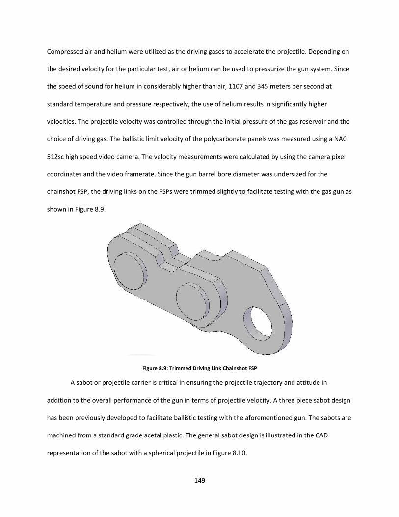
Compressed air and helium were utilized as the driving gases to accelerate the projectile. Depending on
the desired velocity for the particular test, air or helium can be used to pressurize the gun system. Since
the speed of sound for helium in considerably higher than air, 1107 and 345 meters per second at
standard temperature and pressure respectively, the use of helium results in significantly higher
velocities. The projectile velocity was controlled through the initial pressure of the gas reservoir and the
choice of driving gas. The ballistic limit velocity of the polycarbonate panels was measured using a NAC
512sc high speed video camera. The velocity measurements were calculated by using the camera pixel
coordinates and the video framerate. Since the gun barrel bore diameter was undersized for the
chainshot FSP, the driving links on the FSPs were trimmed slightly to facilitate testing with the gas gun as
shown in Figure 8.9.
Figure 8.9: Trimmed Driving Link Chainshot FSP
A sabot or projectile carrier is critical in ensuring the projectile trajectory and attitude in
addition to the overall performance of the gun in terms of projectile velocity. A three piece sabot design
has been previously developed to facilitate ballistic testing with the aforementioned gun. The sabots are
machined from a standard grade acetal plastic. The general sabot design is illustrated in the CAD
representation of the sabot with a spherical projectile in Figure 8.10.
149

Figure 8.10: CAD Representation Of General Sabot Design With Spherical Projectile
The general sabot design was modified to support the chainshot FSP. Figure 8.11 shows the finished
sabot. The sabot has been lengthened and on the interior an oblong profile secures the FSP preflight. A
closer examination of the interior profile is shown in Figure 8.12.
Figure 8.11: Assembled Chainshot FSP Sabot
150

Figure 8.12: Unassembled Chainshot FSP Sabot
It is anticipated that the FSP due to geometry and the moment of inertia will be susceptible to a
significant amount of pitch, roll, and yaw. During the development of the sabot design, 1/4” diameter,
1” long cylindrical rods were used to verify the amount of projectile attitude during flight. The rods were
fired at a velocity of approximately 200 meters per second. The high speed video camera was used to
document the behavior of the projectile and sabot. From the video stills in Figure 8.13, the sabot is
shown to readily separate from the projectile without inducing any attitude. As the sabot further
separates, the projectile maintains its’ trajectory path. The video stills were further analyzed and in all of
the validation performed no more than 5° of pitch were observed where the sabot had a tight fit in the
barrel bore. Thus it was expected that the proposed design would yield similar results for the chainshot
FSP.
151

Figure 8.13: Sabot Design Validation High Speed Video Stills
8.4: Experimental Test Results
8.4.1 : 0.5” Monolithic Lexan Impact Monolithic Lexan panels measuring 6” x 6” x 0.5” (LWD) were impacted with the
aforementioned chainshot FSP using the gas gun. The Lexan panels were clamped around the perimeter
with 0.5” overlap. The FSPs impacted in a trajectory path normal to the panel surface. For the panels
considered, air was used as the driving gas since it yielded sufficient gun performance. The panels were
152

tested at a room temperature of approximately 70° F. A summary of the tests performed are highlighted
in Table 8.1
Table 8.1: 0.5” Monolithic Lexan Chainshot FSP Impact Testing Summary
Based on the testing it is estimated that for the particular testing conditions the ballistic limit velocity of
the monolithic Lexan panel is approximately 282 meters per second. The damage modes observed for
the monolithic Lexan impact testing was plastic deformation and crazing or the generation of
microcracks. The crazing was denoted by a slight discoloration or whitening of the Lexan.
From Test 1 the isometric view of the post-impact damage is presented in Figure 8.14. The FSP
in this case has almost fully perforated the panel. From the damage it is apparent that after the
projectile initial penetrates the Lexan panel, a plastic deformation front forms and progresses through
the thickness of the panel as the projectile moves forward. The plastic deformation front in this case has
taken a mushroom or plug shape. This is similar to the plug formation that occurs in metals under high
velocity impact (9). Wright et al reported the same plugging behavior for thick polycarbonate panels
under impact from cylindrical projectiles (87).
Panel Projectile Panel Projectile Impact Residual1 345.8 6.35 N/A N/A 291.1999 0 Projectile Stuck2 342.15 6.15 341.55 6.15 294.17 128.083 Full Perforation3 343.55 6.2 N/A N/A 281.669 0 Projectile Stuck4 344.15 6.15 343.85 6.25 291.33 83.09 Full Perforation5 344.15 6 343.9 6.05 309.203 143.77 Full Perforation6 340.85 6.05 340.55 6.05 305.689 127.316 Full Perforation
Initial Weight (grams) Residual Weight (grams) Velocity (meters/sec)Test Number
Comments
153

Figure 8.14: 0.5" Monolithic Lexan Post-Impact Damage For Test 1; Isometric View
From Test 4 post-impact damage is shown in Figures 8.15 and 8.16. The predominant damage mode is
plastic deformation. Slight crazing was observed in the direct vicinity of the impact.
Figure 8.15: 0.5" Monolithic Lexan Post-Impact Damage For Test 4; Front Face
154

Figure 8.16: 0.5" Monolithic Lexan Post-Impact Damage For Test 4; Side View
The video stills from Test 5 show that the progression of the pre-impact projectile trajectory.
Minimal attitude is present. In the fifth frame there is a noticeable amount of plastic flow. As the FSP
progresses the plastically deformed plug is driven from the panel and ejected into a small particulate
cloud. After impact the projectile perforates the Lexan panel at an upwards angle. The high speed video
corroborates the progression of the plug formation observed post-impact in Figures 8.14, 8.15, and 8.16.
155

Figure 8.17: 0.5” Monolithic Lexan Impact – Test 5 High Speed Video Stills
8.4.2: 0.75” Laminated Lexan Impact Laminated Lexan panels measuring 6” x 6” x 0.75” (LWD) were impacted using the chainshot FSP
with a normal trajectory path. The laminates Lexan consisted of a central 0.5” thick panel with 0.125”
thick panels adhered to each side. Due to the thickness of the panels, helium was necessary to be able
to fully perforate the panels. The summary of the impact test results for the 0.75” laminated Lexan
panels is shown in Table 8.2.
156

Table 8.2: 0.75" Laminated Lexan Chainshot FSP Impact Testing Summary
Based on the test results it is estimated that the ballistic limit velocity of the laminated Lexan panels is
approximately 425 meters per second. Due to the construction of the laminated panels, the damage
modes present are more complex than in the monolithic case. It was observed that at velocities
significantly lower than the ballistic limit that a substantial amount of delamination, cracking, and plastic
flow occurred. While velocities at or beyond the ballistic limit, plastic flow was the predominant damage
mode.
In Figure 8.18 post-impact damage of Test 1 is shown. The bubble shown is the delamination of
the laminates from the central monolithic panel. Several radial cracks have formed from the center of
the impact point. Also crazing is present on the central monolithic panel as shown in Figure 8.19.
Figure 8.18: 0.75" Laminated Lexan Post-Impact Damage For Test 1; Front Face
Panel Projectile Panel Projectile Impact Residual1 520.05 6.15 N/A N/A 303.66 0 Projectile Stuck2 539.25 6.15 N/A N/A 425.09 0 Projectile Stuck3 540.25 6.05 537.95 464.79 179.27 Full Perforation4 532.55 6.2 532.33 454.18 105.2 Full Perforation5 530.05 6.1 472.98 234.28 Full Perforation6 546.05 6.05 546.1 452 191.81 Full Perforation
Test Number
Initial Weight (grams) Residual Weight (grams) Velocity (meters/sec) Comments
157
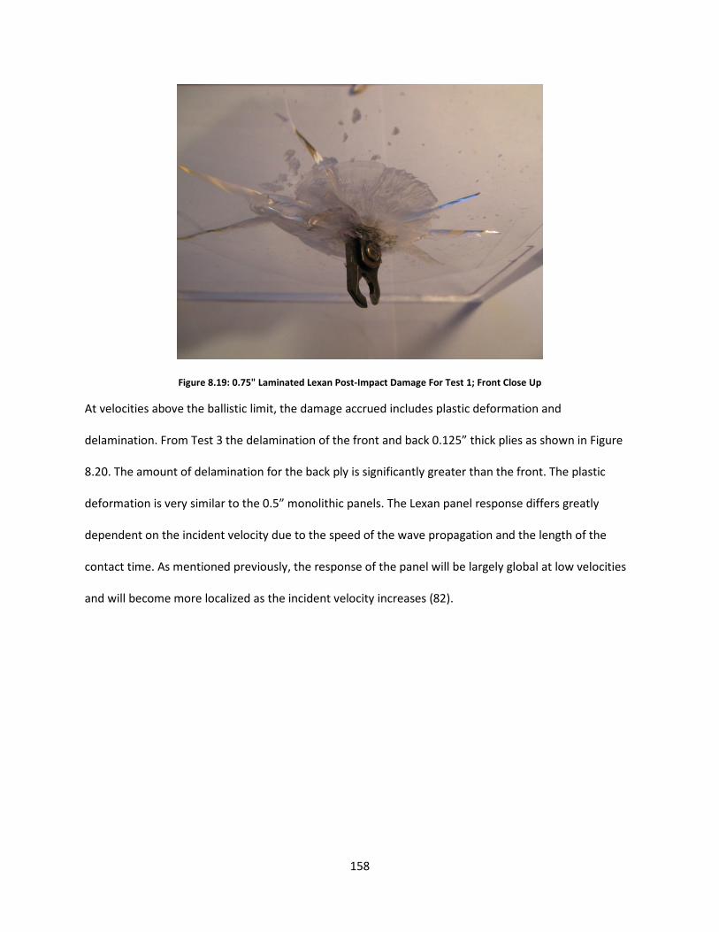
Figure 8.19: 0.75" Laminated Lexan Post-Impact Damage For Test 1; Front Close Up
At velocities above the ballistic limit, the damage accrued includes plastic deformation and
delamination. From Test 3 the delamination of the front and back 0.125” thick plies as shown in Figure
8.20. The amount of delamination for the back ply is significantly greater than the front. The plastic
deformation is very similar to the 0.5” monolithic panels. The Lexan panel response differs greatly
dependent on the incident velocity due to the speed of the wave propagation and the length of the
contact time. As mentioned previously, the response of the panel will be largely global at low velocities
and will become more localized as the incident velocity increases (82).
158

Figure 8.20: 0.75" Laminated Lexan Post-Impact Damage For Test 3; Front Close Up
Figure 8.21: 0.75" Laminated Lexan Post-Impact Damage For Test 3; Back
159

Chapter 9 : Polycarbonate Glazing Ballistic Impact Simulations Finite simulations were developed in LS-DYNA to further explore the chainshot experiments
performed for the Lexan panels. Since many different trajectories and projectile fragments can occur in
chainshot events, there can be a substantial savings for the analyst to develop Finite Element
simulations that can accurately reflect the ballistic impact event. Towards this end, the monolithic case
presented in Section 8.4.1 will be considered. A suitable material model in LS-DYNA to represent the
polycarbonate is explored. Experimental characterization for polycarbonate presented in the literature
is analyzed to develop the material parameters necessary for the ballistic impact simulation. The results
obtained from the simulation are compared to the observations made during testing.
9.1: Polycarbonate Material Behavior Polycarbonate behavior is rate-dependent in addition to being affected by the loading
conditions such as loading direction and ambient temperature. Moy et al performed SPHB testing
comparing the response of Lexan 9034 to increasing strain rates under compressive loads (88). From
Figure 9.1, it is apparent that polycarbonate is rate-dependent exhibits linear elastic, yielding, strain
softening, and strain hardening behavior (88).
Figure 9.1: Polycarbonate Stress-Strain Relationship at Various Strain Rates (Moy et al)
160

Additionally the elastic modulus increases with the strain rate. Li et al studied the strain rate effect of
polycarbonate under compressive dynamic loading conditions using a SPHB setup. The strain rate effects
reported by Li et al are summarized in Table 9.1. It is clear from Figure 9.1 and Table 9.1 the modulus
can be divided by strain rate regime.
Table 9.1: Polycarbonate Strain Rate Effects On Yield Stress And Elastic Modulus (Li et al)
Polycarbonate exhibits a strength differential depending on whether it under compressive or tensile
loading conditions. In Figure 9.2 Boyce et al compared the polycarbonate response under uniaxial
compressive and tensile quasi-static loading (89). There is a clear difference in the stress magnitude
depending on the loading direction.
Figure 9.2: Strength Differential of Polycarbonate (Boyce et al)
Additionally, polycarbonate is also temperature dependent. Richeton et al compared the response
under compressive loads for a range of temperatures as illustrated in Figure 9.3 (90). Comparing Figures
Strain Rate (1/second) Yield Stress (MPa) Elastic Modulus (GPa)4.00E-05 25.2 2.44.00E-02 35 2.4
1200 47.5 5.41700 54.1 5.42200 68.9 5.4
161

9.1 and 9.3, increasing strain rates and decreasing sample temperature both increase the magnitude of
the stress response of polycarbonate.
Figure 9.3: Polycarbonate Stress-Strain Relationship at Various Temperatures at 0.01 / second Strain Rate (Richeton et al)
As a result the yield stress follows the same increasing trend for increasing strain rates and decreasing
temperatures. From Moy et al, Figure 9.4 shows the yield stress increasing to the increasing strain rates
(88). Richeton et al considered yield stress in relation to strain rate and temperature (91). In Figure 9.5
both increasing trends related to strain rate and temperature are observed in the yield stress (91).
Figure 9.4: Polycarbonate Yield Stress As Function of Strain Rate (Moy et al)
162

Figure 9.5: Polycarbonate Yield Stress As Function of Strain Rate and Temperature (Richeton et al)
9.2: LS-DYNA Polycarbonate Ballistic Impact Model Based on the experimental testing outlined in Chapter 8, the LS-DYNA Finite Element model was
created. Figure 9.6 shows the model before impact. Since it was observed in the experimental testing
that the post-impact trajectory of the chain fragment could be unpredictable, symmetry could not be
used to reduce the number of elements in the simulation. A mapped hexahedral mesh for the
polycarbonate panel was created using LS-Prepost. The element size was biased towards the center of
the panel where a finer resolution is needed to capture the highly localized response of the ballistic
impact.
163

Figure 9.6: LS-DYNA FEM Model For Chainshot Impact
The chain fragment consisted of the assembly of five parts: rivets, chain, tie straps, and the driving link.
Due to the geometry of the chain fragment assembly, a mixed mesh of tetrahedral and hexahedral
elements was used. A close-up of the resulting chain fragment assembly mesh is shown in Figure 9.7.
Between each of the individual parts, contact elements are defined to form the assembly. The
*CONTACT_AUTOMATIC_SURFACE_TO SURFACE contact model was defined between each of the chain
fragment components using the standard penalty-based method. For the present model, friction
between the chain components was ignored. As a result of the contact element definitions, the driving
link is able to rotate freely in relation to the assembly. Contact elements were also defined between the
Lexan panel and the chain fragment assembly using *CONTACT_ERODING_SURFACE_TO_SURFACE. The
contact model is also based on the penetration methodology. Additionally it allows for the erosion or
deletion of distorted elements due to the contact model. The static and dynamic friction coefficients
were defined as 0.38 for each (92).
164

Figure 9.7: Chain Fragment Assembly Finite Element Mesh
Under-integrated elements are used in the simulation to reduce the computational cost of the
simulations. As such hourglass control was enabled though the keyword *CONTROL_HOURGLASS to
prevent the non-physical modes that can result when using under-integrated elements.
9.2.1 : Chain Fragment Steel Material Model In the experimental testing no noticeable permanent deformation or damage was observed in
the chain fragments therefore it is assumed that the majority of deformation will be elastic. Additionally
since there is a large difference in modulus between steel and polycarbonate, the chain fragment
deformation will be considered to be largely negligible. Based on the aforementioned assumptions, a
bilinear elasto-plastic material model, *MAT_PLASTIC_KINEMATIC, was used to model the behavior of
the steel chain fragment. The material model parameters for the chain fragment are summarized in
Table 9.2.
165
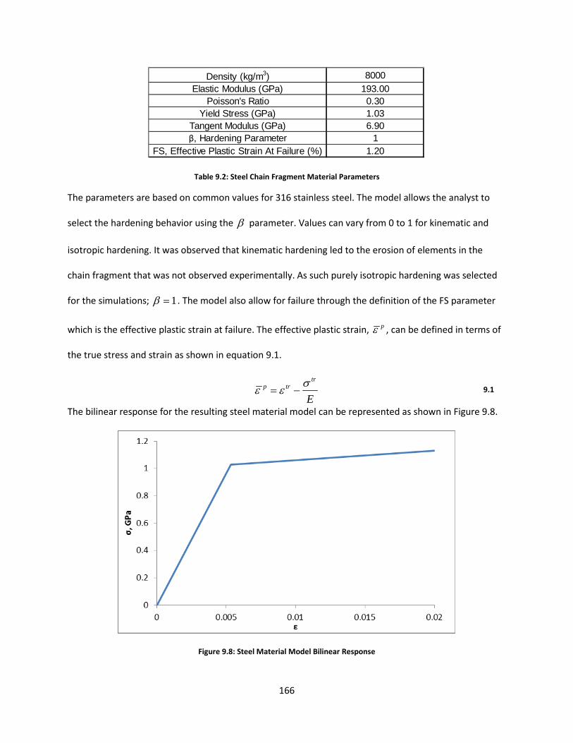
Table 9.2: Steel Chain Fragment Material Parameters
The parameters are based on common values for 316 stainless steel. The model allows the analyst to
select the hardening behavior using the β parameter. Values can vary from 0 to 1 for kinematic and
isotropic hardening. It was observed that kinematic hardening led to the erosion of elements in the
chain fragment that was not observed experimentally. As such purely isotropic hardening was selected
for the simulations; 1β = . The model also allow for failure through the definition of the FS parameter
which is the effective plastic strain at failure. The effective plastic strain, pε , can be defined in terms of
the true stress and strain as shown in equation 9.1.
trp tr
Eσε ε= − 9.1
The bilinear response for the resulting steel material model can be represented as shown in Figure 9.8.
Figure 9.8: Steel Material Model Bilinear Response
Density (kg/m3) 8000Elastic Modulus (GPa) 193.00
Poisson's Ratio 0.30Yield Stress (GPa) 1.03
Tangent Modulus (GPa) 6.90β, Hardening Parameter 1
FS, Effective Plastic Strain At Failure (%) 1.20
166

9.2.2 : Polycarbonate Material Model Given the material behavior observed in the literature summarized in Section 9.1, the strain rate
dependent material model *MAT_STRAIN_RATE_DEPENDENT_PLASTICITY was selected since it can
model the majority of the behavior observed experimentally in Section 9.1. The model is capable of
capturing the rate-dependent behavior but does not include the thermal effects or strength differential.
For the present research, it is assumed that the chainshot impact is an isothermal process so thermal
effects are ignored. Additionally it is assumed that the impact of the strength differential will be
negligible in the overall response.
The model allows for the analyst to define curves to describe the relationship of yield strength,
elastic modulus, and tangent modulus in terms of the effective strain rate (65). The effective strain rate,
ε , can be defined in terms of the deviatoric strain rates, ε ′ , as defined in equation 9.2 (65).
122
3 ij ijε ε ε ′ ′=
9.2
The yield stress in terms of the yield strength, 0σ , elastic modulus, E , tangent modulus, tE , and
effective plastic strain can be defined as in equation 9.3.
( )0p
y p
tp
t
E
whereE EE
E E
σ σ ε ε= +
=−
9.3
Additionally the model has a simple material failure option by allowing the analyst to define a failure
curve in relation to the effective strain rate. The failure curve can be defined in terms of either the
effective or Von-Mises stress , effective plastic strain, maximum and absolute value of the principal
stresses, or the maximum principal stresses at failure (65). The effective stress and effective plastic
strain can be defined as shown in equations 9.4 (5) and 9.5 (70), respectively. The effective plastic strain
is in terms of the true stress and strain for a uniaxial load.
167

( ) ( ) ( ) ( )
122 2 2 2 2 2
11 22 22 33 33 11 12 23 311 32
σ σ σ σ σ σ σ σ σ σ = − + − + − + + + 9.4
p trtr E
σε ε= − 9.5
The material parameters for the polycarbonate are summarized in Table 9.3. The density and
poisson’s ratio were obtained from the manufacturer datasheet for Lexan 9034 (93). As mentioned
earlier a curve relating the elastic modulus with the effective strain rate can be defined. However this
option is not recommended in LS-DYNA (65). As such a constant elastic modulus is defined. Since high
strain rates are expected during the ballistic impact event, the elastic modulus is based on the values
reported by Li et al for high strain rates.
Table 9.3: Polycarbonate Material Constants
In order to define the curves relating yield strength and tangent modulus to effective strain rate, the
data from Richeton et al (90) was considered. The material model takes the discrete curve data and
interpolates for intermediate values. In order to reduce the amount of interpolation required, a curve fit
was used for the dataset in order to provide a continuous and smooth representation of the
relationships. In Figures 9.9 and 9.10, the strain rate effects for the yield stress and tangent modulus are
plotted. The nonlinear regression was performed on the experimental data using power law
relationships for strain rates ranging from 1E-3 to 3000 per second. The model fit obtained for the curve
was excellent. Since it is unknown whether the strain rate relationships will follow the same
relationships as shown in Figures 9.9 and 9.10, the last calculated datapoint was used for strain rates
above 3000 per second to form a piecewise function. Curve data was generated for strain rates ranging
from 1E-3 to 1E+7 per second.
Density (kg/m3) 1200Elastic Modulus (GPa) 5.00
Poisson's Ratio 0.37
168

Figure 9.9: Polycarbonate Yield Stress As A Function of Strain Rate
Figure 9.10: Polycarbonate Tangent Modulus As A Function of Strain Rate
As mentioned earlier, the model allows for the analyst to define material failure through several
different options. For the current research failure was defined in terms of the effective plastic strain in
relations to the corresponding strain rate. The failure strains are calculated by determining the plastic
169

strain using the uniaxial data from Richeton et al (90) and Moy et al (88). After converting the failure
strains back to engineering strain from true strain, the relationship based on strain rate can be
summarized as in Table 9.4. Due to the difficulty of developing a smooth curve through a regression
model fit, a piecewise step function was defined for the material model using the experimental data.
Table 9.4: Polycarbonate Effective Plastic Strain at Failure Versus Strain Rate
9.3: LS-DYNA Simulation Results The simulations were performed at the impact velocities for each of the experimental tests
outlined in Section 8.4.1. The relationship between the impact and residual velocities are summarized in
Figure 9.11 for both the experimental and simulation results. As shown in the plot, the LS-DYNA
simulations are in good agreement with the experimental test for impact velocities above 290 meters
per second. As the model approaches closer to the ballistic limit velocity, a larger discrepancy in the
residual projectile velocity is observed. The FEM model predicts a ballistic limit of approximately260
meters per second compared to 281.67 determined experimentally. The 7.7% percent difference for the
ballistic limit is a good first estimation since limited experimental data was available for the yield stress,
tangent modulus, and failure strain curves.
Strain Rate Failure Strain1.00E-03 1.801.00E-01 1.70
10 1.403000 0.654600 0.50
170

Figure 9.11: 0.5" Monolithic Lexan Ballistic Impact Experimental Vs. FEM Comparison
In the simulations, the plugging behavior observed experimentally during the impact event was
recreated. A comparison of the high speed video stills to the corresponding simulation output is
depicted in Figure 9.12 for Test 5 of the monolithic testing matrix. After impact plastic deformation
initiates and progresses as the chain fragment continues to penetrate the panel. As more plastic
deformation occurs, the plug size continues to increase. After perforation the plug is ejected from the
panel. Figure 9.13 shows the progression of the effective plastic strain for the cross-section of the Lexan
panel. Simulation stills 1 and 2 clearly show the plastic plug formation observed experimentally in Figure
8.14. The remaining stills show the ejection of the plastic plug and the plastic zone evolution as the
chain fragment further perforates the panel.
171

Figure 9.12: Comparison Of Experimental And LS-DYNA Ballistic Event for Test 5 of Monolithic Testing
172
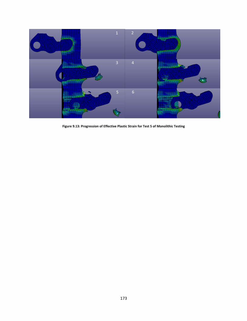
Figure 9.13: Progression of Effective Plastic Strain for Test 5 of Monolithic Testing
173

Chapter 10 : Conclusions The preceding chapters have covered the experimental and numerical methods developed and
utilized throughout the course of the research studying ballistic impact of polymeric composites and
polymers. The experimental portion of the research included the development of the ballistic impact
test equipment and procedures, comparison between thermoplastic and epoxy based composites for
ballistic performance, development of the falling object hazard test, and ‘chainshot’ polycarbonate
impact. The numerical analysis included the derivation of a coupled viscoplastic progressive damage
composite material model, development of an optimization algorithm to determine the composite
model parameters, implementation of the aforementioned model into the explicit integration FEM
solver LS-DYNA, and validation of the LS-DYNA implementation for various loading conditions.
A single stage gas gun system has been developed and utilized for several test programs.
Through continuous improvement activities, the gun is capable of accelerating 1/4" diameter steel
spherical projectiles consistently within a velocity range of 100 to 800 meters per second at a high level
of target accuracy. By maintaining a modular system design, the gun is capable of accommodating a
wide range of projectile sizes through the standard and upsized barrel configurations. Due to the
simplicity of both the sabot design and corresponding manufacturing processes, asymmetrical projectile
geometries can also be accelerated with a true trajectory and minimal attitude. The velocity calculation
GUI for the high speed camera video data demonstrated that it can readily handle the video files
typically produced during the different ballistic impact testing programs. The current implementation
utilizes very simple image preprocessing techniques for identification of the projectile. Future works
should consider more advanced routines which can also predict the trajectory path based on previous
data and subdivide the pixel data for a quicker grid search of the projectile. This would help minimize
the amount of preprocessing necessary while also allowing for the tracking of multiple objects
simultaneously.
174

It was observed in the thermoplastic comparison that there is a significant performance
advantage for thermoplastic based composites over the epoxy based subject to high velocity impact.
Since, in the present research, replication was not utilized, a significant difference within the
thermoplastic and epoxy matrix classes could not be established. A larger sample size would be
necessary to quantify the difference. The upsized gun configuration developed for the large object
falling hazard test program was capable of accelerating the 1-3/8” diameter steel sphere to a velocity of
150 feet per second at an acceptable level of accuracy. Prior to future testing programs, the target
fixture and safety enclosure will both need to be further stiffened to eliminate or significantly reduce
the amount of deflection observed during the initial testing. The gas gun was also used for the
‘chainshot’ impact against monolithic and laminated polycarbonate panels. The experimentally-
determined ballistic limit velocity of 282 meters per second for the considered monolithic case is in
agreement with the reports made by the chain manufacturer. Using published experimental material
characterization data for polycarbonate, the ‘chainshot’ event for 0.5” thick monolithic Lexan panel was
simulated using a strain rate dependent plasticity model. The simulation results were able to recreate
the plastic plug formation observed experimentally in the polycarbonate panels. Additionally the model
predicted a ballistic limit velocity of approximately 260 meters per second. This is a reasonable estimate
of the ballistic limit for monolithic polycarbonate panels.
A 3-D coupled viscoplastic progressive damage material model suitable for simulation of the
ballistic response of composite materials was developed with the intent of implementation into the
Finite Element software, LS-DYNA. The model describes the nonlinear behavior exhibited by composites
through both the plasticity and progressive damage models. The composite material model
algorithmically couples the plastic and damage models through a return mapping integration scheme
where the viscoplastic model response is corrected by the damage model. Based on literature
recommendations and published experimental data for a common aerospace-grade composite material,
175

the maximum strain criteria was selected for determining the onset of damage. The damage model uses
a bilinear energy balance approach for the dissipation of the intralaminar and interlaminar fracture
energies of the composite material. In order to couple the fracture mechanics and the continuum
damage mechanics frameworks, a 3-D smeared crack model was utilized. The smeared crack model
represents the microcracks with the composite by a characteristic length relative to the element size. A
benefit to the smeared crack model is that the energy dissipation of a composite structure predicted by
the model will not be as sensitive due to the level discretization in the Finite Element simulation.
The composite material model was implemented into the commercial FEM software, LS-DYNA,
for model validation and ballistic simulation. A common aerospace-grade composite, IM7/8552 carbon
fiber/epoxy, was presented as an example for model validation. Since the viscoplastic model is
generalized to accommodate a wider range of composite constituents, there are more material
parameters to determine. In order to ease the use of the model, a simple optimization algorithm was
developed to determine the viscoplastic model parameters. The example case was then validated
through a series of simulations to examine the behavior of the viscoplastic, progressive damage, and
smeared crack algorithms within the composite material model. The simulations demonstrated that for
the IM7/8552 example the model was able to reproduce the majority of the nonlinear behavior
demonstrated in the published characterization data. However for off-axis loading, the maximum strain
criteria did not predict the amount of damage observed experimentally for the larger angles. This
limitation is mainly attributed to the estimation of the failure shear strain since it was desired to avoid
the use of exaggerated shear strain values. For future research efforts, further development is necessary
for the failure criteria utilized. Also the model demonstrated minimal variation in the fracture energy
dissipation when comparing the sensitivity to different levels of mesh refinement and distortion.
Based on the validation of the material model for the considered IM7/8552 case, ballistic testing
published in the literature was simulated for the prediction of both the ballistic limit velocity and center
176

panel deflection. The simulation result was within a reasonable margin with the experimentally
determined ballistic limit velocity. The model predicted velocity of 87.06 meters per second compared
with approximately 97 meters per second reported in the literature. However the model under-
predicted the central panel deflection predicted with a value of 1.75 millimeters at 107 microseconds
after impact. This discrepancy in the predicted panel deflection is largely attributed to the perfect bond
assumption made between each of the plies made for computational efficiency and that the material
model parameters were developed with only in-plane behavior. The damage associated with shear in
the 2-/3-plane for the 54 meters per second case simulation exhibited a similar pattern to what is
observed experimentally in ultrasonic testing. As anticipated, for each of the plies the orientation of the
damage coincided with the ply orientation.
177

References 1. Stilp, A. J. and Hohler, V. Experimental Methods for Terminal Ballistics and Impact Physics. [book auth.] Jonas A. Zukas. High Velocity Impact Dynamics. s.l. : John Wiley & Sons, Inc., 1990, pp. 515-592.
2. Development of a three-stage, ligh-gas gun at the University of Dayton Research Institute. Piekutowski, A.J., Poorman, K.L. s.l. : International Journal of Impact Engineering, 2006, Vol. 33.
3. Fox, Robert W. and McDonald, Alan T. Introduction to Fluid Mechanics. s.l. : John Wiley & Sons, Inc., 1998. ISBN 0-471-12464-8.
4. Seigel, Arnold E. The Theory of High Speed Guns. s.l. : United States Naval Ordinance Laboratory, 1965.
5. Ugural, Ansel C. and Fenster, Saul K. Advanced Strength And Applied Elasticity. s.l. : Prentice Hall, 2009.
6. NAC Image Technology. NAC HotShot 512sc User's Manual. 2010.
7. Hypervelocity impact daamge prediction in composites: Part I-material model and characterisation. Clegg, R.A., White, D.M., Riedel, W., Harwick, W. s.l. : International Journal of Impact Engineering, 2006, Vol. 33.
8. Hypervelocity impact daamge prediction in composites: Part II-experimental investigations and simulations. Riedel, W., Nahme, H., White, D.M., Clegg, R.A. s.l. : International Journal of Impact Engineering, 2006, Vol. 33.
9. Nicholas, Theodore and Recht, Rodney F. Introduction to Impact Phenomena. [book auth.] Jonas A. Zukas. High Velocity Impact Dynamics. s.l. : John Wiley & Sons, Inc., 1990.
10. Zukas, Jonas A. Introduction to Penetration Mechanics. High Velocity Impact Dynamics. s.l. : John Wiley & Sons, Inc., 1990.
11. Recht, Rodney F. High Velocity Impact Dynamics: Analytical Modeling of Plate Penetration Dynamics. [book auth.] Jonas A. Zukas. High Velocity Impact Dynamics. s.l. : John Wiley & Sons, Inc., 1990.
12. Ballistic Perforation Dynamics. Recht, R.F. and Ipson, T.W. s.l. : Journal of Applied Mechanics, 1963, Vol. 30.
13. Lambert, J. P. and Jonas, G. H. Towards Standardization in Terminal Ballistics Testing: Velocity Represention. Aberdeen Proving Grounds, MD : Ballistic Research Laboratories, 1975.
14. On the Lambert-Jonas approximation for ballistic impact. Ben-Dor, G., Dubinsky, A. and Elperin, T. 29, s.l. : Elsevier Science Ltd., 2002, Vol. Mechanics Research Communications.
178

15. Ferriter, E. Andrew, McCulloh, Ian A. and DeRosset, William. Techniques Used to Estimate Limit Velocity in Ballistics Testing with Small Sample Size. s.l. : U.S. Army Aviation School.
16. Silsby, G. Penetration Mechanics of Anti-Armor Kinetic Energy Penetrators. s.l. : LAB-R-GFS871, 1987.
17. Renegade Materials Corporation. RM-2005 Toughned Epoxy (Product Data Sheet). 2012.
18. Hexcell. HexPly 8552 Epoxy Matrix Product Data. 2014.
19. Tencate. Datasheet Tencate Cetex PPS.
20. —. Datasheet Tencate Cetex PEI.
21. Terminal Ballisitics Of Composite Panels and Verfication of Finite Element Analysis; Masters Thesis. Grupp, J.S. Auburn : Auburn University, 2011.
22. A Simple Flow Rule for Characterizing Nonlinear Behavior of Fiber Composites. Sun, C. T. and Chen, J. L. 10, s.l. : Journal Composite Materials, 1989, Vol. 23.
23. Srinivasa, Arun R. and Srinivasan, Sivakumar M. Inelasticity Of Materials: An Engineering Approach and a Practical Guide. s.l. : World Scientific, 2009. ISSN: 1793-0901.
24. A theory of the yielding and plastic flow of anisotropic metals. Hill, R. 1033, s.l. : Proceedings Of The Royal Society London A, 1948, Vol. 193.
25. A Quadratic Yield Function for Fiber-Reinforced Composites. Chen, J. K., Allahdadi, F. A. and Sun, C. T. 8, s.l. : Journal Of Composite Materials, 1997, Vol. 31.
26. Model for the strain-rate-dependent behavior of polymer composites. Thiruppukuzhi, Srikanth V. and Sun, C. T. s.l. : Composites Science and Technology, 2001, Vol. 61.
27. Use of split Hopkinson pressure bar testing off-axis composites. Ninan, Lal, Tsai, J. and Sun, C. T. s.l. : International Journal Of Impact Engineering, 2001, Vol. 25.
28. Constitutive model for high strain rate response of polymeric composites. Tsai, J. and Sun, C. T. s.l. : Composites Science and Technology, 2002, Vol. 62.
29. Modeling Non-Linear Rate-Dependent Behavior In Fiber-Reinforced Composites. Weeks, C. A. and Sun, C. T. 3-4, s.l. : Composites Science and Technology, 1998, Vol. 58.
30. Crash energy absorption of braided composite tubes. Flesher, Nathan D. s.l. : Thesis, Stanford University, 2005.
31. A dynamic crash model for energy absorption in braided composite materials. Part I: Viscoplastic material model. Flesher, Nathan D., Chang, Fu-Kuo and Janapala, Nageswara R. 8, s.l. : Journal Of Composites Materials, 2011, Vol. 45.
179

32. A dynamic crash model for energy absorption in braided composite materials - Part II: Implementation and verification. Flesher, Nathan D., Chang, Fu-Kuo and Janapala, Nageswara R. 8, s.l. : Journal Of Composite Materials, 2011, Vol. 45.
33. Crashworthiness of Composite Structures with Various Fiber Architectures. Janapala, Nageswara R., et al., et al. Detroit : 11th International LS-DYNA Users Conference, 2010.
34. The effects of strain rate on the mechanical behaviour of kevlar fibre bundles: an experimental and theoretical study. Wang, Yang and Xia, Yuanming. s.l. : Composites Part A, 1998, Vol. 29 A.
35. A Plastic Potential Function Suitable for Anisotropic Fiber Composites. Chen, J.L. and Sun, C.T. 14, s.l. : Journal Of Composite Materials, 1993, Vol. 27.
36. Micro-mechanical Model with Strain-Rate Dependency and Damage for Impact Simulation of Woven Fabric Composites. Tabiei, Ala and Ivanov, Ivelin. s.l. : Mechanics of Advanced Materials and Structures, 2007, Vol. 14.
37. Hyer, Michael W. Stress Analysis Of Fiber-Reinforced Composite Materials. s.l. : McGraw-Hill, 1998. 0-07-016700-1.
38. Simo, J.C. and Hughes, T.J.R. Computational Inelasticity. New York : Springer-Verlag, 1998. 0-387-97520-9.
39. Belytschko, Ted, Liu, Wing Kam and Moran, Brian. Nonlinear Finite Elements for Continua and Structures. West Sussex : John Wiley & Sons Ltd., 2000. 0-471-98773-5.
40. A Universal Integration Algorithm For Rate-Dependent Elastoplasticity. Fotiu, P.A. and Nemat-Nasser, S. 6, s.l. : Computers & Structures, 1996, Vol. 59.
41. An Analysis Of A New Class Of Integration Algorithms For Elastoplastic Constitutive Relations. Ortiz, M and Simo, J.C. s.l. : International Journal For Numerical Methods In Engineering, 1986, Vol. 23.
42. Viscoplasticty For Instabilities Due To Strain Softening And Strain-Rate Softening. Wang, W.M., Sluys, L.J. and De Borst, R. s.l. : International Journal For Numerical Methods In Engineering, 1997, Vol. 40.
43. Ramsey, Fred and Schafer, Daniel. The Statistical Sleuth: A Course In Methods Of Data Analysis. s.l. : Cengage Learning, 2002. 978-0534386702.
44. High strain rate characterisation of unidirectional carbon-epoxy IM7-8552 in transverse compression and in-plane shear using digital image correlation. Koerber, H, Xavier, J. and Camanho, P.P. s.l. : Mechanics Of Materials, 2010, Vol. 42.
45. Prediction of size effects in notched laminates using continuum damage mechanics. Camanho, P.P., Maimi, P. and Davila, C.G. s.l. : Composites Science and Technology, 2007, Vol. 67.
46. An energy based damage mechanics approach to modelling impact onto woven composite materials: Part I. Numerical models. Iannucci, L., Willows, M.L. s.l. : Composites: Part A, 2006, Vol. 37.
180

47. A Three-Dimensional Ply Failure Model for Composite Structures. Donadon, M.V., Almeida, S.F.M., Arbelo, M.A., Faria, A.R. s.l. : International Journal of Aerospace Engineering, 2009, Vol. 2009.
48. Kachanov, L.M. Introduction to Continuum Damage Mechanics. Brookline, MA : Martinus Nijhoff Publishers, 1986. 90-247-3319-7.
49. A combined elastoplastic damage model for progressive failure analysis of composite materials and structures. Chen, J.F., Morozov, E.V., Shankar, K. s.l. : Composite Structures, 2012, Vol. 94.
50. LS-DYNA Implementation of Polymer Matrix Composite Model Uner High Strain Rate Impact. Zheng, X., Goldberg, R.K., Binienda, W.K., Roberts, G.D. s.l. : NASA 2003-212583, 2003.
51. High strain rate characterisation of unidirectional carbon-epoxy IM7-8552 in longitudinal compression. Koerber, H., Camanho, P.P. s.l. : Composites: Part A, 2011, Vol. 42.
52. Crack Band theory for fracture of concrete. Bazant, Z.P., Oh, B.H. s.l. : Materials and Structures, 1983, Vol. 16.
53. A Consistent Characteristic Length For Smeared Cracking Models. Oliver, J. s.l. : International Journal For Numerical Methods In Engineering, 1989, Vol. 28.
54. A continuum damage model for composite laminates: Part I - Constitutive model. Maimí, P., Camanho, P.P., Mayugo, J.A., Dávila, C.G. s.l. : Mechanics of Materials, 2007, Vol. 39.
55. A continuum damage model for composite laminates: Part II - Computational implementation and vaildation. Maimí, P., Camanho, P.P., Mayugo, J.A., Dávila, C.G. s.l. : Mechanics of Materials, 2007, Vol. 39.
56. Progressive damage modeling in fiber-reinforced materials. Lapczyk, I., Hurtado, J.A. s.l. : Composites: Part A, 2007, Vol. 38.
57. An Objectivity Algorithm for Strain Softening Material Models. Donadon, M.V., Iannucci, L. Dearborn, MI : 9th International LS-DYNA Users Conference, 2006.
58. A progressive failure model for composite laminates subjected to low velocity impact damage. Donadon, M.V., Iannucci, L., Falzon, B.G., Hodgkinson, J.M., de Almeida, S.F.M. s.l. : Computers and Structures, 2008, Vol. 86.
59. Ballisitic Impact Modeling of Composite Materials. Yen, Chian-Fong. 7th International LS-DYNA Users Conference.
60. A ballisitc material model for continuous-fiber reinforced composites. Yen, Chian-Fong. s.l. : Internation Journal of Impact Engineering, 2012, Vol. 46.
61. Lai, Michael W., Rubin, David and Krempl, Edward. Introduction To Continuum Mechanics. s.l. : Butterwortk-Heinemann;Elsevier, 2010. 978-07506-8560-3.
181
62. CDPM2: A damage-plasticity approach to modelling the failure of concrete. Grassl, Peter, et al., et al. s.l. : International Journal Of Solids And Structures, 2013, Vol. 50.
63. A Fully Coupled Elasto-Viscoplastic Damage Theory For Anisotropic Materials. Zhu, Y.Y., Cescotto,S. 11, s.l. : International Journal of Solids and Structures, 1994, Vol. 32.
64. Testing and modeling high strain rate behavior of polymeric composites. Thiruppukuzhi, S.V and Sun, C.T. s.l. : Composites Part B, 1998, Vol. 29B.
65. (LSTC), Livermore Software Technology Corporation. LS-DYNA Keyword User's Manual Version 971. s.l. : (LSTC), Livermore Software Technology Corporation, 2007.
66. Auburn University College of Engineering. vSMP HPCC - Virtual Symmetric Multiprocessing High Performance Compute Cluster description. Auburn University College of Engineering. [Online] February 9, 2011. [Cited: July 21, 2014.] http://www.eng.auburn.edu/admin/ens/hpcc/hpcc-description.html.
67. Tensile mechanical behavior of T300 and M40J fiber bundles at different strain rate. Zhou, Yuanxin, Jiang, Dazhi and Xia, Yuanming. s.l. : Journal Of Materials Science, 2001, Vol. 36.
68. American Society for Testing and Materials (ASTM). ASTM D3039/D3039M-00 Standard test method for tensile properties of polymer matrix composite materials.
69. Jones, Robert M. Mechanics Of Composite Materials. s.l. : Taylor & Francis, 1999. ISBN: 1-56032-712-X.
70. (LSTC), Livermore Software Technology Corporation. LS-DYNA Theory Manual. s.l. : (LSTC), Livermore Software Technology Corporation, 2006.
71. Hexcell. HexTow IM7 Product Data. 2014.
72. —. HexTow Carbon Fiber. 2014.
73. Material Sciences Corporation (MSC). MAT 162 Material Model Users Manual V1.0. 2010.
74. The effect of shear strength on the ballisitic response of laminated composite plates. Karthikeyan, K., Russell, B.P., Fleck, N.A., Wadley, H.N.G., Deshpande, V.S. s.l. : European Journal of Mechanics A/Solids, 2013, Vol. 42.
75. A Novel Fluid Structure Interaction Experiment to Investigate Deformation of Structural Elements Subjected to Impulsive Loading. Espinosa, H.D., Lee, S., Moldovan, N. s.l. : Experimental Mechanics, 2006, Vol. 46.
76. A heuristic attempt to reduce transverse shear locking in fully integrated hexahedra with poor aspect ratio. Borvall, T. s.l. : 7th European LS-DYNA Conference, 2009.
77. Wear of Steel Against Carbon Fibre Reinforced PPS. Quintelier, Samyn, P., De Baets, Ost, W., Van Paepegem, W. 3 & 4, s.l. : Tribology In Industry, 2005, Vol. 27.
182

78. Coefficient of friction for aluminum in contact with a carbon fiber epoxy composite. Schön, Joakim. s.l. : Tribology International, 2004, Vol. 37.
79. Machinery for forestry - Glazing and panel materials used in operator enclosures for protection against thrown sawteeth - Test Method and performance criteria. International Organization for Standardization (ISO). Vol. ISO 11839:2010.
80. Normal missile penetration and perforation of layered plates. Radin, J and Goldsmith, W. s.l. : International Journal of Impact Engineering, 1988, Vol. 7.
81. D3763-10: Standard Test Method for High Speed Puncture Properties of Plastics Using Load and Displacement Sensors. American Society for Testing and Materials (ASTM). 2010.
82. Zukas, Jonas A. Introduction to Hydrocodes. s.l. : Elsevier Science, 2004. ISBN: 0-08-044348-6.
83. Oregon Products North America. Chain Shot. Oregon Products North America. [Online] 2013. [Cited: July 31, 2014.] http://www.oregonproducts.com/harvester/service/chain_shot.htm.
84. Oregon Products. Oregon Mechanical Timber Harvesting Handbook. Portland, Oregon : s.n., 2005.
85. Washington State Department of Labor Industries. Timber Harvester Operator Killed Following a Chain Shot Incident. 2014. Investigation # 10WA04801; SHARP Report # 52-30-2014.
86. Johansson, Louise, Hallonborg, Ulf and Granlund, Paul. Chain shot - clear road ahead for development and testing of shot guards. s.l. : Skogforsk, The Forestry Institute of Sweden, 2004.
87. Ballisitic Impact Of Polycarbonate - An Experimental Investigation. Wright, S.C., Fleck, N.A. and Stronge, W.J. 1, s.l. : International Journal of Impact Engineering, 1993, Vol. 13.
88. Strain Rate Response Of A Polycarbonate Under Uniaxial Compression. Moy, P., et al., et al. Charlotte, NC : Proceedings of SEM Annual Conference on Experimental Mechanics, 2003.
89. An experimental and analytical investigation of the large strain compressice and tensile response of glassy polymers. Boyce, M.C. and Arruda, E.M. 20, s.l. : Polymer Engineering & Science, 1990, Vol. 30.
90. Influence of temperature and strain rate on the mechanical behavior of three amorphous polymers: Characterization and modeling of the compressive yield stress. Richeton, J., et al., et al. s.l. : International Journal of Solids And Structures, 2006, Vol. 43.
91. Constitutive modeling of polymer matierials at impact loading rates. Richeton, J., et al., et al. s.l. : J. Phys. IV France, 2006, Vol. 134.
92. American Society for Metals (ASM). Appendix: Static and Kinetic Friction Coefficients for Selected Materials. [book auth.] American Society for Metals (ASM). ASM Handbook. 1992.
93. General Electric Structured Products. Lexan 9034 Sheet Product Data Sheet. 1998.
183

184


