
ESD.77 FINAL PROJECT SPRING 2010
Barge Design Optimization Anonymous MIT Students
Abstract— In this project, three members of the Armed Forces tested the multi-disciplinary system design optimization approach to concept evaluation on a simplified platform, a barge. A barge is a non-self propelled vessel that incorporates the basic disciplines of ship building: hydrodynamics, hydrostatics, and structural mechanics. Using four bounded design variables, we attempt to optimize the payload, in tons, that a barge could carry within the physical constraints. We conduct a design of experiments to select an initial design to further optimize. Sequential quadratic programming (SQP) was used to solve the non-linear program (NLP) in computer software MATLAB. The NLP was also solved using the genertic algorithm (GA) heurisitic. SQP converged quickly and found the optimal solution. The problem was expanded to include another objective, structural weight. The multi-objective problem was solved to create a Pareto front to show the trade-offs for each objective. The results of the study show this approach is feasible for these types of platforms and allow the opportubnity for expansion of included disciplines as well as increased fidelity of the model used. Thus, eventually, a warship or some other such complex system could be designed with this approach.
Index Terms—Barge, MDO, SQP, Genetic Algorithm
—————————— ——————————
1 INTRODUCTION
barge is a typically non-self propelled , flat-
bottomed vessel used initially for river or canal
transportation of heavy goods. Although other
means of transportation have been developed since their
introduction, barges are still used all over the world as a
low-cost solu tion for carrying either low -value or heavy
and bulky items.
Although a barge is very simplistic compared to most
of its waterborne brethren, it still presents ample oppor-
tunity to experiment with balanced designs. A customer
may desire to carry as much payload as possible to gain
effeciencies in their transportation costs, but maximizing
these payloads must be balanced by engineers to operate
within the laws of physics (including stability, buoyancy,
powering, resistance, structures, etc.) and balanced by
financiers to operate within a customer ’s allowable limits
of cost. These two very obvious considerations alone can
create quite a complex balancing act, since these forces -
requirements, feasibility, cost - tend to oppose each other.
2 MOTIVATION
The team’s interest and background in many asso-
ciated d isciplines has primarily motivated this project.
During the team’s tenure at Massachusetts Institu te of
Technology, they have taken a range of courses inclu ding
Marine Hydrodynamics, Design Principles for Ocean Ve-
hicles, Principles of Naval Architecture, Power and Pro-
pulsion, Structural Mechanics, Plates and Shells, Ship
Structural Analysis and Design, and Ship Design and
Construction. Each of these courses had one of two ap-
proaches. Either the course examined a particular d iscip-
line of ship design and mentioned that a designer should
not forget other d isciplines, or the course examined the
design as a process and recognized the many disciplines
but encouraged an iterative, ―throw -it-over-the-wall‖ ap-
proach to converge to a point design. To further emphas-
ize, even the courses that recognized the multi-
d isciplinary aspects of ship design only designed for con-
vergence to any feasible design within the space, not nec-
essarily an optimal design.
Thus, the team wished to explore the possibility of an
optimal design amongst each of the d isciplines. We
wanted to create an optimal design from a multi-
d isciplinary standpoint and understand the associated
trade-offs within the design vector. Meanwhile, we
wanted to acquire knowledge and skills by using the m e-
thods and tools of this new trade.
The team knew, however, that using these tools to d e-
sign any standard sea-going vessel would provide d im i-
nishing returns due to the incredibly complex and
coupled nature of the entire set of design variables. Thus,
the team used a simplified , low -fidelity model on a sim-
ple vessel – a barge – to demonstrate the benefit of these
tools within the marine design environment. The under-
standing was that the design vector could grow and th e
fidelity of the model could increase modularly to accom-
modate increasingly complex designs for more typical
ocean platforms. Indeed, two team members have the
task of performing a clean slate design of a warship for
the next year, so, should they incorporate these tools in
the design process, the d esign vector will grow and the
ESD.77 © 2010 IEEE
————————————————
Student A is pursuing a Naval Engineer’s Degree and an MS in Engi-neering Management through the Systems Design and Management pro-gram, both at the Massachussetts Institute of Technology in Cambridge, MA 02139.
Student B i s pursuing a Naval Engineer’s Degree and an MS in
Engineering Management through the Systems Design and Management program, both at the Massachussetts Institute of Technology in Cambridge, MA 02139. Student C is pursuing an MS in Operational Research at Massachu-
setts Institute of Technology in Cambridge, MA 02139.
A

2 ESD.77 FINAL PROJECT SPRING 2010
fidelity and computational expense of the model will in-
crease very quickly. This project proved a good proof of
concept for the team members to grow and add variables,
parameters, constraints, and fidelity to at a later date.
3 PROBLEM FORMULATION
As with any vessel operating in the marine environ-
ment, the designer has to deal with stability, seakeeping
and structural strength issues – to name a few - all of
which come from different d isciplines: hydrostatics, hy-
drodynamics, and structural mechanics. The team used
the methods and tools of multi-d isciplinary system d e-
sign optimization to optimize the design of a barge with
respect these d isciplines. The primary design objective
was to maximize the payload (i.e. the cargo capacity) that
the barge can effectively carry. Eventually, this project also
balanced that optimization against the cost of the vessel,
represented by the barge’s weight .
To start, the team utilized a MATLAB® code imple-
mented to model a barge’s seakeeping behavior (the hy-
drodynamics of the vessel) during a Design Princip les of
Ocean Vehicles term project. The code was limited to non-
self-propelled vehicles, and only evaluated heave and
pitch motions. The original code also only studied one
particular hull shape with a particular beam to draft ratio.
Out of a desire to eliminate d iscrete variables, the hydro-
dynamic properties represented in the code for each beam
to draft ratio were first fitted to curves in order to allow
for a continuous design space exploration instead of limit-
ing the beam to be either 2-, 4-, or 8- times the draft of the
barge.
Additionally, the team modeled the hydrostatics and
structural strength of the barge. The hydrostatics re-
quirements and implementation were derived from Prin-
ciples of Naval Architecture, and provided the basic re-
quirements that the barge float (buoyancy equals weight)
and that it floats upright (positive metacentric height).
The structural mechanics module was derived from the
American Buereau of Shipping (ABS) ru les for steel ves-
sels assuming mild steel as the type of m aterial.
Originally, the team designated 8 design variables to be
changed during the exporation of the design space. These
variables were length, beam, draft, depth, vertical center
of gravity (VCG), speed, cross-sectional area coefficient,
and d isplacement. However, cross-sectional area coeffi-
cient was a result of beam and draft, so it was elim inated
and only used as an intermediate variable. Also, d is-
placement and VCG were a result of length, beam, draft,
and the payload – our objective – so they were eliminated
as design variables, also, and only used as an interm e-
diate variables. Because draft was also a result of payload ,
it was eliminated as a design variable. Finally, speed was
removed as a design variable because it only affected the
hydrodynamics, not the hydrostatics or structural m e-
chanics, so the team thought it uninteresting to explore at
this time, besides the fact that typically a speed is desig-
nated as a requirement by a cu stomer.
Thus, the remaining design variables for this project
were:
The length (L)
The beam (B)
The depth (D)
The thickness of the steel plates (t)
The bounds for our design variables are typical of
barges.
Additionally, implementation of the code required
several other inputs that the team considered fixed for the
purposes of this exploration. These parameters were re-
quired by one or more modules to adequately model the
appropriate responses of the modules to the design vec-
tor. These design parameters were:
The significant wave height of the assumed
ocean cond itions (H)
Peak spectral frequency of the assumed
ocean cond itions (ω)
Mild steel material density (ρ)
Young’s Modulus of mild steel (E)
The longitud inal position of the center of
gravity (LCG)
Sea-water density (ρsw
)
Fresh water density (ρfw
)
Like any typical engineering problem, the team recog-
nized there would be constraints that limited our poten-
tial solu tion set. Steel beams and plates cannot extend to
infinite without buckling under their own weight at some
point, let alone sustain added pressure from a payload
without buckling. Other physical constrainsts were ac-
counted for. There were also assumed customer con-
straints, for instance the frequency that the customer
would allow the cargo to get wet given the assumed sea
state. The team did their best to account for several physi-
cal and customer constraints on this problem, finally end-
ing with:
Inequality constraints:
Design Parameters Value Unit
v Speed 10 knots
kg Payload vertical center of gravity 1.2D
lcg Payload longitudinal center of gravity 0.5L
ω Peak spectral frequency 0.7 rad/sec
H Signif icant wave height 2.5 m
ρ Sea water density 1025 kg/m3
ρstr Material thickness 7850 kg/m3
3-1: Design Variables and Bounds
3-2: Design Parameters and Values

ESD.77 FINAL PROJECT SPRING 2010 3
The maximum allowable stresses for the
deck and the keel in sagging, hogging and
calm water cond itions must be less than or
equal to the critical stress of mild steel
Initial metacentric height greater than
0.15m for initial stability (Limit set by
American Bureau of Shipbuild ing (ABS)
rules)
Occurrences of green water on deck less
than or equal to one every minute
The draft must be less than 6m, a reason a-
ble depth for a d redged channel or river
The wid th mu st be less than 35m in order
to fit in certain locks along seaways
Equality constraints were:
Buoyancy must equal the weight (floating
condition)
Because the model was greatly simplified , the Design
Structure Matrix (DSM) representation of each of the p a-
rameters and variables within each of the modules was
also rather simple to see. We were able to remove itera-
tions and loops using only one iteration through the
DSM, as noted from Figure 1 to Figure 2 below.
The analysis routines include the evaluation of the
three d isciplines modules. The hydrostatic module com-
prises calculations for determining the position of the
barge’s center of gravity in its loading condition . This is
then used to determine the vertical metacentric height
(GM), which is the most representative stability index.
This implementation evaluates GM that has to be greater
than 0.15m according to the ABS rules.
The structural analysis module evaluates ABS-derived
parametric equations to determine the maximum stresses
in hogging and sagging wave cond itions. This assumes a
uniform longitudinal weight d istribution, which is not
expected to be always true in real-case scenarios but is a
reasonable assumption within the scope of this project .
Maximum bending moment stresses are experienced in
the deck and keel edges and these particular values are
evaluated against the stress limit for mild steel, which is
our material choice.
The hydrodynamic module evaluates the seakeeping
behavior of the barge. Seakeeping analysis is limited in
the coupled heave and pitch responses and the output is
the number of occurrences of green water on deck per
hour. For this project we have set the constraint to be less
than sixty. Pitch and heave motions are calculated based
on 2D strip theory and are evaluated against head seas.
The local hydrodynamics properties are based on exper i-
mental measurements from Lewis form theory. The neces-
sary curve fitting is implemented to allow for a cont i-
nuous design space exploration . Seakeeping is evaluated
for the Bretschneider spectrum with a significant wave
height of 3m and peak spectral frequency of 0.7rad/ sec.
This choice of spectrum may not be ideal for a barge
project design since it is most applied for fu lly developed
seas but still is adequate for the purpose of this project .
The basic input/ output d iagram is depicted below in
Figure 3. There are several intermediate variables and
parameters, as mentioned, but this simple d iagram cap-
tures the design variables, the outputs of the modules,
and the subsequent calculation of our objectives using
those outputs.
The program starts from zero payload and performs
iterations until the maximum payload is achieved for a
specific design vector without violating any constraint in
a Multi-d isciplinary Feasible (MDF) aproach. At the same
time the structural weight necessary to implement this
design is calculated , this value can be used as a surrogate
Inequality Constraints
N<60 Number of occurences of green water on deck per hour
T<6m Draft
GM>0.15m Metacentric height
B<30m Beam <30m to f it through Panama Canal
σk,sag<250MPa Keel stress at sagging wave
σk,hog<250MPa Keel stress at hogging wave
σd,sag<250MPa Deck stress at sagging wave
σd,hog<250MPa Deck stress at hogging wave
Design Vector Const Vector Hydrodynamics Hydrostatics
Structural
Mechanics
1-6,8 1-5,8 1-5
20,21,25,26,27 23,25-27 22-24
7 7
Figure 1: Initial DSM
Design Vector Const Vector Hydrostatics Hydrodynamics
Structural
Mechanics
1-5,8 1-6,8 1-5
23,25-27 20,21,25,26,27 22-24
7 7
Figure 2: Final DSM Figure 3: Input/Output Diagram with Modules
3-3: Inequality Constraints

4 ESD.77 FINAL PROJECT SPRING 2010
result for the cost of the vessel.
4 VALIDATION
The code was used in analysis mode to validate its re-
sults against a known barge, the MARMAC 400, found
with Macdonough Marine Service. This benchmarking
gave good confidence in the model and the results. Our
design vector was:
122m length
30m beam
6.1m depth
16mm thickness
The analysis code gave the results of:
4.35m load line draft
14,670MT payload
These results compare very well with the MARMAC
400. The characteristics of this existing barge are:
121.92m length
30.4m beam
6.1m depth
4.34m load line draft
11,453.9MT payload
Initially, there was concern that the team’s result for
payload was significantly higher (28% higher) than this
existing barge. However, upon further inspection of the
characteristics of the MARMAC 400, there are d ifferences
that can explain a good portion of this d ifference. For in-
stance, the modeled barge was an exact square box with
an inner bottom for added structural strength. The
MARMAC 400 is not a perfect box; it has shaped bow and
edges. This decreases the volume of the MARMAC 400
compared to the model.
Additionally, the MARMAC 400 does not have an in-
ner bottom for added strength. The team postu lates that
the MARMAC 400 could be limited in the capacity it can
carry due to its structural members; the shell might
buckle earlier and thus have hogging or sagging stresses
in the deck or keel as a limiting factor, whereas the active
constraint of the model was the number of occurances of
water on deck. Additionally, the MARMAC 400 likely has
more structural members in the form of plate stiffeners
and girders that likely increase the structural weight of
that vessel compared to ours, which will also increase the
hogging and saggin moments of that vessel compared to
ours, which in trun decrease the payload.
Lastly, the payload characteristic of the MARMAC 400
is based on operations, where the segmentation of the
stores on the MARMAC 400 limits its capacity. O perators
could overcome this limitation by stacking cargo higher,
but then would run into the metacentric height constraint
for stability. Contrastingly, the model has no segmenta-
tion, and assumes a uniformly d istributed load both lon-
gitudinally and athwartship throughou t the vessel (un-
iformly d istributed d irt, or sugar cane, or concrete, for
instance). This aspect allows the model to fit more pay l-
oad in the vessel with a lower metacentric height of the
vessel-payload system.
Thus, with these considerations in mind, the team con-
sidered the model adequate enough for evaluation pu r-
poses. Additionally, the team recognized that these d iffer-
ences and real world constraints would scale with the
barge, so that any optimal solu tion would remain the op-
timal solu tion with the above considerations, even though
the payload may not be exact.
5 INITIAL DESIGN SPACE EXPLORATION
An initial exploration of the design space was carried
out using a fractional factorial design . We d iscretized the
remaining four continuous design variables to three levels
– high, medium, and low. For simplicity, the team chose
the high values to be the upper bounds of each of the d e-
sign variables, the low values to be the lower bounds of
the variables, and the medium values to be the midpoint
of the bounds. A fu ll factorial design would mean 34=81
experiments. At the time, the team was only interested in
the main effects and two-way interactions, so a fractional
factorial design was selected instead .
Thus, the team completed 48 runs. Sixteen of these
runs returned infeasible results, and were eliminated ,
leaving 32 runs to analyze. The results of these 32 runs
were used in JMP® statistical software to determine the
main effects. The results, in Figure 4 below, conclude that
the beam had the most significant effect on the payload ,
and length and depth had about half as much affect. The
values for length and beam had very high confidence le-
vels, while the draft was quite widely d istributed . This
gave the team good confidence in the model, but, more
importantly, gave a good starting point for the numerical
optimizations.
Specifically, the starting point used during optimiza-
tion, based on the results of the DOE, was:
140m length 30m beam 9m depth 20mm plate thickness
6 OPTIMIZATION ALGORITHMS
6.1 Gradient-based Optimization: SQP
We selected Sequential Quadratic Programming (SQP)
for our grad ient-based optimizer. MATLAB uses this al-
gorithm in the function ―fmincon.‖ The barge model uses
a multi d isciplinary feasible (MDF) approach that builds
the equality and inequality constraints into the subsystem
modules. Subsequently, no constraints are handled by the
optimization algorithm at the system level.
The bounds on the design variables make the optimi-
Figure 4: Design Variable Estimates from JMP®

ESD.77 FINAL PROJECT SPRING 2010 5
zation process challenging using an unconstrained algo-
rithm. MATLAB’s ―fminsearch‖ and ―fminunc‖ functions
were available to use Steepest Descent, Quasi-Newton, or
Newton’s method but would require a formulation to
penalize the objective function when the design variables
fell outside of the feasible region (ou tside of the design
variable bounds). Introducing penalties for bounds viola-
tion would introduce complexity in the optimization a l-
gorithm. Consequently, the team selected ―fmincon‖ as
the most effective and elegant way to input bounds for
the design variables and optimize the model.
6.2 Single Objective Optimization: Payload
Payload was selected as the single objective function to
be optimized . Between payload and structural weight, we
believe that the process of optimizing the payload will
provide better insights for the design process. Moreover,
payload seems to be more d irectly coupled with all con-
straints.
Convergence of the algorithm was achieved only a fter
the convergence tolerance on the model was significantly
reduced . High convergence tolerance initially cau sed the
optimization algorithm to finite d ifference noise and fail .
When we specified a smaller convergence tolerance, the
optimization algorithm yielded the local optimum in the
order of 20-25 iterations with a random starting point .
Starting from
20
9
35
140
0x
where the DOE found the best
solu tion. After 16 iterations the algorithm yielded:
78.15
2.8
35
140
*x
as the optimal solution, resulting in a payload of 24,358
tons. Compared to the initial starting point payload of
23,757 tons, the optimal had an increase in 601 tons.
The optimal barge maintains the maximum length and
beam, but is 0.7 meters less deep, and 4.22 mm less plate
thickness. The DOE showed, and w e expected , the largest
boat in length and beam to provide the largest payload
possible. The solver confirmed that and d id not move
from the upper bound on length and beam . The decrease
in the last two variables, depth and p late thickness, pro-
duced a more efficient ship , mainly because of structural
considerations. Reducing plate thickness applies to the
entire barge so even a small reduction brings down over-
all barge weight. Any lessening in hull thickness needs to
maintain the structural constraints, such as maximum
allowable stresses at a hogging wave, but will also reduce
the weight that goes into the hydrostatic constraints. The
solver found the thinner hall, with a reduced depth, was
still feasible and reduced the barge weight allowing for
additional payload .
The algorithm yielded a moderate improvement . Tak-
ing into account that our starting point was the best est i-
mation from the DOE, the small amount of improvement
seems reasonable.
6.3 Sensitivity Analysis
The gradient of the objective function at the optimal
solu tion was:
140
16
717
10*62.1 6
J
Figure 5 shows the normalized sensitivities for each
design variable after normalization around the optimal
solu tion.
The length (L) has the significant effect. This agrees
with intu ition; the size of the barge has a significant effect
on the payload capacity of the barge. This finding streng-
thens our notion that SQP found the optimal solu tion .
Any increase in length has a large impact on im proving
the objective; the SQP solu tion was the upper bound of
length. As long as constraints are not v iolated , the most
length will be used . We expected to experience similar
results with beam, but found that it had little impact.
The plate thickness (t) slightly decreases the payload as
it increases. This also follows intu ition . Any additional
thickness of the hull will increase the barge weight, and
will not allow the same amount of payload to meet stru c-
tural constraints.
Two of the constraints were active at the optimal solu-
tion, the number of occurrences of green water on deck
per hour (N) and deck stress at hogging wave (σd ,hog
).
We manually extracted the parameter sensitivity. The
output arguments of the optimization algorithm could
not provide this because we used an MDF implementa-
tion -- all constraints were handled within the model. This
is a d isadvantage of MDF implementation of the model.
The manually extracted parameter sensitivity showed
us the impact of speed, v, as seen in the Figure 6. The con-
straint of green water on deck is highly dependent on
speed . The increase of speed will cause more green w ater
Figure 5: Normalized Sensitivites for Design Variables

6 ESD.77 FINAL PROJECT SPRING 2010
on deck and violate the constraint. The violation of the
constraint because of faster spped could be remedied by
decreasing the payload or the size of the barge (which
would also decrease the payload).
The parameters payload vertical center of gravity (kg)
and significant wave height (H) also had negative impact
on the overall payload . An increase in either parameter
would also impact the number of green waves on deck ,
but not as significantly as speed .
6.4 Heuristic Optimization
We used a Genetic Algorithm on maximize barge payl-
oad . The team expected the GA to be easiest heuristic to
understand and implement. Moreover, the fitness func-
tion implementation was straightforward for our max-
imization problem and w ithout necessity to include any
constraints. Finally, the bounds of the design variables
can be set within the algorithm.
Although the GA was expected to be computationally
expensive, we decided to leverage the probabilistic transi-
tion ru les it u ses for a more robust design space explor a-
tion.
Our first attempt to implement the GA yielded results
comparable to the gradient-based SQP we used in the
previously. Specifically, the best fitness occurred at:
1.25
9.8
6.34
7.138
*gax
resulting to P = 22,468 tons compared to 24,358 tons at
2.14
7.8
35
140
*SQPx
from the grad ient-based SQP.
The GA appeared to stop near a local optimal that was
much thicker than the SQP solu tion (10.9 mm greater).
The thicker hull probably required a smaller boat so the
length and beam were reduced . This p late thickness was
actually greater than the 20 mm we used from the DOE.
This GA implementation used crossover rate of 1, m u-
tation rate of 0.03 and 16 bit encoding for all design v a-
riables. This encoding corresponds to a precision higher
than 10-2 for all design variables based on
xxUB xLB
2bits and drives the population size.
A second attempt was made by at 0.02 mutation rate.
The results were comparable to the first GA implementa-
tion but d id not reach the gradient-based SQP implemen-
tation.Namely, the best fitness occurred at
29.24
99.8
97.34
77.139
*gax with P = 23,060 tons.
Both GA runs exceeded 10 hours to evaluate 100 gen-
erations. The noticeable d ifference between GA and SQP
was the plate thickness (t). Both GA implementations
pointed higher thicknesses but the lower thickness found
from the SQP yields higher payload and follows intu ition
as explained previously. Additional GA tuning was seen
unnecessary.
6.5 Global Optimum
Running the optimization with d ifferent starting points
resulted in d ifferent optimum solu tions. This reveals that
our design space is non-linear. Although, after leveraging
the DOE results, we expected SQP to have found the
global optimum, we were cautious since SQP is inherently
incapable of dealing with local optima and we had indica-
tions that there may be m any in this design problem . GA
implementation pointed towards this d irection even
though it d id not succeed in reaching the optimum with
good accuracy.
The global optimum is thus estimated at:
2.14
7.8
35
140
*SQPx
where P = 24,358 tons.
7 POST-OPTIMALITY ANALYSIS
The calculated Hessian matrix using second order fi-
nite d ifferencing for a stesize of 10-4 at the optimal solu-
tion was
[2.4473x10¹²
2.44731x10¹²
2.44695x10¹²
2.44695x10¹²
]
Altough these entries were very high, they still were of
the same order and subsequent attempt to scale the d e-
sign variables d id not provide any improved results. This
was expected as the convergence history was fairly
straightforward as depicted in Figure 7. The function ap-
proaches convergence at the sixth iteration of the algo-
Figure 6: Normalized Sensitivites of Design Parameters
ESD.77 FINAL PROJECT SPRING 2010 7
rithm.
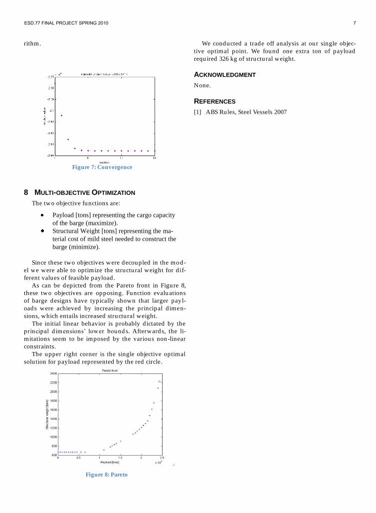
8 MULTI-OBJECTIVE OPTIMIZATION
The two objective functions are:
Payload [tons] representing the cargo capacity
of the barge (maximize).
Structural Weight [tons] representing the ma-
terial cost of mild steel needed to construct the
barge (minimize).
Since these two objectives were decoupled in the mod-
el we were able to optimize the structural weight for d if-
ferent values of feasible payload.
As can be depicted from the Pareto front in Figure 8,
these two objectives are opposing. Function evaluations
of barge designs have typically shown that larger pay l-
oads were achieved by increasing the principal d imen-
sions, which entails increased structural weight.
The initial linear behavior is probably d ictated by the
principal d imensions’ lower bound s. Afterwards, the li-
mitations seem to be imposed by the various non -linear
constraints.
The upper right corner is the single objective optimal
solu tion for payload represented by the red circle.
We conducted a trade off analysis at our single objec-
tive optimal point. We found one extra ton of payload
required 326 kg of structural weight.
ACKNOWLEDGMENT
None.
REFERENCES
[1] ABS Rules, Steel Vessels 2007
Figure 7: Convergence
Figure 8: Pareto

MIT OpenCourseWarehttp://ocw.mit.edu
ESD.77 / 16.888 Multidisciplinary System Design OptimizationSpring 2010 For information about citing these materials or our Terms of Use, visit: http://ocw.mit.edu/terms.


