
Bioconductor and R for preprocessing and analyses of
genomic microarray data
Tanya Logvinenko, PhD
Biostatistician
Children’s Hospital Boston

Bioconductor • Open source software project for analyses
and comprehension of high-throughput genomic data
http://www.bioconductor.org/

Bioconductor
• Based on R statistical programming language
• R
– Free, open source
• Need R installed to use Bioconductor

R References
• “Modern Applied Statistics with S” (4th edition, 2005) by Venables and Ripley (outdated but still relevant); ISBN: 0387954570
• “R for Beginners” on CRAN website http://cran.r-project.org/doc/contrib/Paradis-rdebuts_en.pdf
• “A beginners Guide to R” by Zuur, Leno & Meesters; ISBN:
0387938362
• “R manuals” on CRAN website http://cran.r-project.org/manuals.html
– An Introduction to R (mainly)

Bioconductor References
• “Bioinformatics and Computational Biology Solutions Using R and Bioconductor” (2005) by Genteleman, Carey, Huber, Irizarry and Dudoit; ISBN: 0387251464
• “Bioconductor Case studies” (2008) by Hahne, Huber, Genetleman & Falcon; ISBN: 0387772391
• Workflows on Bioconductor website http://www.bioconductor.org/help/

R Installation
• From:
http://cran.r-project.org/
• Choose latest version
– try to not use versions .0
• Download executable
• Follow prompts to install

R programming language
• q() – command to quit R

R Programming
• Start R
• Open New Script (File -> New Script) – Type and keep all your code saved in the script file

R programming
• In the editor can type commands
• Highlight commands and press Ctrl R to execute
• To stop execution Press “Stop” button or “Esc”
• To open new Editor press Ctrl N
• To save commands press Ctrl S

R Programming
• Setting working directory – Create a special folder, e.g. C:\GenCourse
– Command will set your working directory setwd(“C:/GenCourse/”);
• Note the change from \ to /!
• This is where we will have data and will keep work!
• To check working directory use function getwd()

R Programming
• R is case sensitive – myData and Mydata are different names!!! – In names can use alphanumerics, “_” and “.”
• Names need to start with a letter
• Assignment operators are “<-” or “=“
x<-2 #assigns to x a value of 2
y<-c(1,2,3) #assigns to y a vector of length 3
• Comments can be typed after hash # (to the end of
line)
R Programming
• Everything in R is an object
• R creates and manipulates objects: – Variables, matrices, functions, etc.
• Every object has a class
– ’character’: a vector of character strings – ’numeric’: a vector of real numbers – ’integer’: a vector of integers – ’logical’: a vector of logical (true/false) values – ’list’: a vector of R objects

R Programming
# Vectors
x.vec <- seq(1,7,by=2)
names(x.vec) <- letters[1:4]
y.Vec <- x.vec*4+3;
# Matrices
x.mat <- cbind(x.vec, rnorm(4), rep(5, 4))
y.mat <- rbind(1:3, rep(1, 3))
z.mat <- rbind(x.mat, y.mat)
# Data frames
x.df <- as.data.frame(x.mat)
names(x.df) <- c(’ind’, ’random’, ’score’)

R Programming • Accessing elements # Access first element of ’x.vec’
x.vec[1]
# or if you know the name
x.vec[’a’]
# Access an element of ’x.mat’ in the second row,
# third column
x.mat[2,3]
# Display the second and third columns of
# matrix ’x.mat’
x.mat[,c(2:3)]
# or
x.mat[,-c(1)]
# What does this command do?
x.mat[x.mat[,1]>3,]
# Get the vector of ’ind’ from ’x.df’
x.df$ind
x.df[,1]

R Programming
• Modifying elements # Change the element of ’x.mat’ in the third
row
# and first column to ’6’
x.mat[3,1] <- 6
# Replace the second column of ’z.mat’ by
0’s
z.mat[,2] <- 0
R Programming
• Sorting, might want to re-order the rows of a matrix or see the sorted elements of a vector
# Simplest ’sort’
z.vec <- c(5,3,8,2,3.2)
sort(z.vec)
order(z.vec)

R Programming Bracket Function
() For function calls f(x) and to set priorities 3*(2+4)
[] For indexing purposes in vectors, matrices, data frames
{} For qrouping sequences of commands {mean(x); var(x)}
[[]] For list indexing

R Programming
• Getting help with functions and features help(hist)
?hist
help.search(’histogram’)
help.start()
example(hist)
• The last command will run all the examples included
with the help for a particular function. If one wants to run particular examples, can highlight the commands in the help window and submit them by pressing Ctrl V

R Programming
• Graphics – Univariate:
• hist() • stem() • boxplot() • density()
– Bivariate
• plot()
– Multivariate • pairs()

R Programming
• Libraries
– R has packages called “libraries” which can be installed and used.
– In R,choose Packages -> Install Packages
– Choose CRAN mirror
– Choose package
– Once package (e.g., gplot) loaded library(gplots) #library gplots is loaded

BioConductor Installation
• Load BioConductor source("http://bioconductor.org/biocLite.R")
• Load a library
– Affy for preprocessing/analysis of Affymetrix oligo arrays
biocLite("affy")
library(affy)

Affymetrix Data
• We will work with a subset of the data on Down Syndrome Trisomy 21
– Mao R, Wang X, Spitznagel EL Jr, Frelin LP et al. Primary and secondary
transcriptional effects in the developing human Down syndrome brain and heart. Genome Biol 2005;6(13):R107. PMID: 16420667
• Experiment with Affymetrix® GeneChip™ Human U133A arrays
• The raw data for this study is available as experiment number GSE1397 in the Gene Expression Omnibus: http://www.ncbi.nlm.nih.gov/geo/

Working with data in R/Bioconductor
• Zipped data is in http://sites.tufts.edu/cbi/resources/geneexpressionanalysis/
• Extract data in your special course directory
• Check the directory where the .CEL files are
• In R set this as your working directory – Remember to change / to \!!!
Working with Affy data
• Installing Bioconductor packages
biocLite("affy")
biocLite("affycoretools")
• Loading affy and affycoretools packages into our R environment:
library(affy)
library(affycoretools)
Read/Pre-process
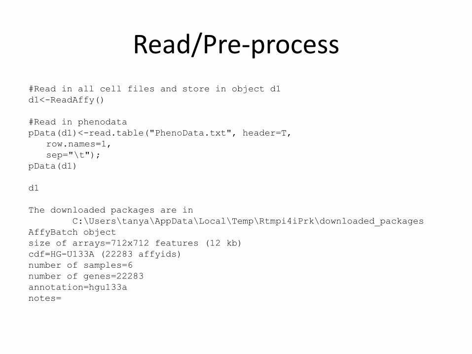
#Read in all cell files and store in object d1
d1<-ReadAffy()
#Read in phenodata
pData(d1)<-read.table("PhenoData.txt", header=T,
row.names=1,
sep="\t");
pData(d1)
d1
The downloaded packages are in
C:\Users\tanya\AppData\Local\Temp\Rtmpi4iPrk\downloaded_packages
AffyBatch object
size of arrays=712x712 features (12 kb)
cdf=HG-U133A (22283 affyids)
number of samples=6
number of genes=22283
annotation=hgu133a
notes=

image(d1[,1])

hist(d1)
6 8 10 12 14
0.0
0.1
0.2
0.3
0.4
log intensity
de
nsity

boxplot(d1)
Down.Syndrome.Cerebellum.1218.1.U133A.CEL Normal.Cerebellum.1411.1.U133A.CEL
68
10
12
14

plot(exprs(d1)[,1], exprs(d1)[,2])

Normalization
• Background correction
• Normalization
• Probe-set expression extraction
– RMA
– GC-RMA
– MAS5 (Affymetrix)
– MBEI
– …

Normalization
• RMA
eset.rma <- rma(d1) #RMA to normalize the data and
extract probe-set intensity
• MAS5
eset.mas <- mas5(d1) #MAS5 to normalize the data
and extract probe-set intensity

Normalization
• GC-RMA – In Bioconductor package “gcrma”
biocLite(“gcrma”)
library(gcrma)
eset.gcrma <- gcrma(d1) #GC-RMA to normalize the data and
extract probe-set intensity
• MBEI (algorithm from dChip, Li-Wong) – In affy library
eset.dchip <- expresso(d1, normalize.method=“invariantset”,
bg.correct=TRUE, pmcorrect.method=“pmonly”,
summary.method=“liwong”) #MBEI to normalize the data
and extract probe-set intensity
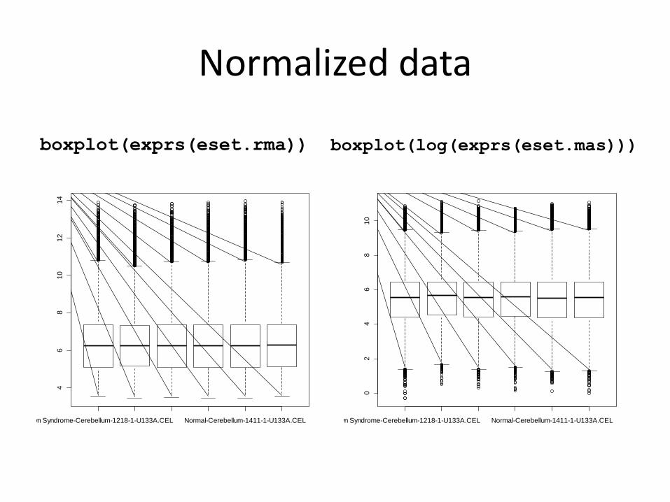
Normalized data
boxplot(exprs(eset.rma))
Down Syndrome-Cerebellum-1218-1-U133A.CEL Normal-Cerebellum-1411-1-U133A.CEL
46
81
01
21
4
boxplot(log(exprs(eset.mas)))
Down Syndrome-Cerebellum-1218-1-U133A.CEL Normal-Cerebellum-1411-1-U133A.CEL
02
46
81
0

Differential Expression
• Genes differentially expressed between Down Syndrome and normal samples
• Use library “limma” biocLite("limma");
library(limma)
plotPCA(eset.rma, groups =
as.numeric(pData(d1)[,1]),
groupnames =
levels(pData(d1)[,1]))
-10 0 10 20 30
-10
-50
51
0
Principal Components Plot
PC1
PC
2
DownSyndrom
Normal

Differential expression • Create a design matrix for analysis (compare Normal to Down Syndrome) pData(d1)[,1 ]
[1] DownSyndrom DownSyndrom DownSyndrom Normal Normal Normal
Levels: DownSyndrom Normal
group<- factor(pData(d1)[,1 ] , levels = levels(pData(d1)[,1]))
design<- model.matrix(~group)
(Intercept) groupNormal
1 1 0
2 1 0
3 1 0
4 1 1
5 1 1
6 1 1

Differential Expression
• Fit linear model to each gene – The data is in eset.rma
– Model matrix is design fit1 <-lmFit(eset.rma, design)
• Get p-values for comparisons fit1 <-eBayes(fit1)
Gets significance attached to the estimated coefficients. Uses that all genes were present across all arrays to obtain better estimates of statistical significance. Important to not forget this step!!!

Differential Expression
• Create a list of 50 genes with strongest differential expression (highest significance)
tab50 <- topTable(fit1, coef = 2, adjust = "fdr",
n = 50)
• Option coef=2 means we are looking at the coefficient for β in the model, the one corresponding to the difference between Normals and Down Syndrome samples
• Option adjust=“fdr” means we adjust for multiple testing – very important!!!
• View the top two rows of the created table head(tab50, n=2)

Adjustment for Multiple testing
• With multiple genes tested simultaneously (22K in our case) at 5% significance level we expect 5% of the genes to show differential expression just due to chance (in case there is really NO genes with differential expression).
• To correct it need to adjust for multiple testing

Adjustment for Multiple testing
p.adjusted<-p.adjust(p.values, method =“BH”)
• Available methods for adjustment
– Controlling for False Discovery Rate (expected number of false positives) – more powerful • “BH” (or “fdr”): Benjamini-Hochberg • “BY”: Benjamini-Yakuteli
– Controlling for Family-Wise error rate – less powerful • “bonferroni”: very conservative (Bonferroni) • "holm“: less conservative (Holm, ‘79) • "hochberg“: less conservative (Hochberg, ‘88) • "hommel”
– "none“
• These methods are available in topTable() function

Differential Expression
head(tab50, n=2) ID logFC AveExpr t P.Value adj.P.Val B
18842 219478_at -0.5145739 7.408018 -7.644772 6.267949e-05 0.5022679 0.6624038
9620 210136_at -1.2367957 6.372380 -7.549204 6.851779e-05 0.5022679 0.6216099
ID =probe-set logFC =log of Fold Change (Normal toDownSyndrome) logFC (DownSyndrome to Normals)is negative of it AveExpr = average expression across all arrays t =t-statistic P.Value = p.value comparing Normal to Down Syndrome group
for a gene Adj.P.Val =adjusted for multiple testing p-value B =log-odds ratio for differential expression

heatmap(exprs(esetSel))

Pretty Heatmap
library(gplots)
colMy=c("green", "magenta");
heatmap.2(exprs(esetSel),
trace="none",
ColSideColors=colMy[
as.numeric(as.numeric(group))],
labRow="",
cexCol=0.6, scale="row",
col=redgreen,
main="Significant Genes with p-
value < 0.001")

Pretty Heatmap Code
• Library where function heatmap.2 is – library(gplots)
• Spedicifcation of colors for identification of cases – colMy=c("green", "magenta");
• Option trace="none“ removes trace across each array
• Option ColSideColors=colMy[
as.numeric(as.numeric(group))] assigns the colors to vertical bar at the top, green (1st color to DownSyndrome (determined by alphabetical order of groups)
• Option scale="row“ scales gene expressions across arrays to have mean 0 and standard deviation 1
• Option col=redgreen for heatmap in green/red instead of default red/yellow

Annotation
probeList <- rownames(exprs(eset.rma));
if (require(hgu133a.db) & require(annotate))
{
geneSymbol <- getSYMBOL(probeList, 'hgu133a.db')
geneName <- sapply(lookUp(probeList, 'hgu133a.db',
'GENENAME'), function(x) x[1])
EntrezID <- sapply(lookUp(probeList, 'hgu133a.db',
'ENTREZID'), function(x) x[1])
}

Annotation
numGenes <- nrow(eset.rma);
annotated_table <- topTable (fit1, coef=2, number=numGenes,
genelist=fit1$genes);
#note logFC is between Normals and DownSyndrome; change it
annotated_table$logFC <- -annotated_table$logFC;
annotated_table$FC <- ifelse (annotated_table$logFC > 0,
2^annotated_table$logFC, -1/2^annotated_table$logFC);
colnames(annotated_table)
[colnames(annotated_table)=="FC"] <-
"FoldChange DownS/Norm";

Annotation
UP_annotated_table <-
annotated_table[(annotated_table[,
"FoldChange DownS/Norm"] > 0),]
DOWN_annotated_table <-
annotated_table[(annotated_table[,
"FoldChange DownS/Norm"] < 0),]
write.table (UP_annotated_table,
file="Upregulated in DS genes_all.txt",
sep="\t",quote=FALSE,row.names=F);
write.table (DOWN_annotated_table,
file="Downregulated in DS genes_all.txt",
sep="\t",quote=FALSE,row.names=F);

Illumina Bead Array Data
• Need libraries from Bioconductor
– limma
– lumi
– genefilter
– Mapping info library (Human is lumiHumanAll.db)
– gplots

Illumina Analyses
Set working directory (where your data is) setwd("C:/Users/tanya/Desktop/GenCourse/Illumina");
Load libraries (if not installed need to call Bioconductor and install them using biocLite() function library(limma);
library(lumi);
library(genefilter);
library(lumiHumanAll.db)
library(gplots)
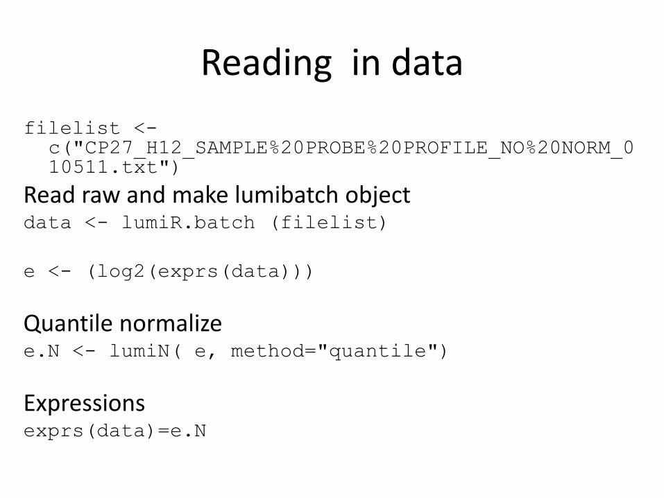
Reading in data
filelist <- c("CP27_H12_SAMPLE%20PROBE%20PROFILE_NO%20NORM_010511.txt")
Read raw and make lumibatch object data <- lumiR.batch (filelist)
e <- (log2(exprs(data)))
Quantile normalize e.N <- lumiN( e, method="quantile")
Expressions exprs(data)=e.N

• We will consider only those probes that are present in all 20 arrays
presentCount <- detectionCall(data, Th=0.05)
sele.N1<- e.N[presentCount==20,]
selprobeList <- rownames(sele.N1)
probeList <- rownames(e.N)

Annotation
if (require(lumiHumanAll.db) & require(annotate)) {
geneSymbol <- getSYMBOL(probeList, 'lumiHumanAll.db')
selgeneSymbol <- getSYMBOL(selprobeList, 'lumiHumanAll.db')
geneName <- sapply(lookUp(probeList, 'lumiHumanAll.db', 'GENENAME'), function(x) x[1])
EntrezID <- sapply(lookUp(probeList, 'lumiHumanAll.db', 'ENTREZID'), function(x) x[1])
selgeneName <- sapply(lookUp(selprobeList, 'lumiHumanAll.db', 'GENENAME'), function(x) x[1])
}
e.Nsel=e.N[rownames(e.N) %in% selprobeList,];
dim(e.Nsel)

Design of Experiment
des=read.table("Design.txt", sep="\t",
header=T);
head(des)
des=des[,1:7];
des=des[order(des$SampleID),];
des$SampleID == colnames(e.Nsel)
#YES, otherwise order e.Nsel columns by
colnames.

Analysis (Model Building)
TumorType=as.factor(des$TumorType);
Patient=as.factor(des$Patient);
tp=model.matrix(~-1+TumorType+Patient);
tp
fit1 <- lmFit(e.Nsel,design=tp)
boxplot (as.data.frame
(fit1$coefficients))

Comparison between groups
?makeContrasts
contr1=makeContrasts(TumorTypeDL-TumorTypeL,
TumorTypeDL-TumorTypeLP,
TumorTypeDL-TumorTypeM, TumorTypeDL-TumorTypeUN,
TumorTypeL-TumorTypeLP, TumorTypeL-TumorTypeM,
TumorTypeL-TumorTypeUN, TumorTypeLP-TumorTypeM,
TumorTypeLP-TumorTypeUN, TumorTypeM-TumorTypeUN,
levels=c("TumorTypeDL", "TumorTypeL", "TumorTypeLP",
"TumorTypeM", "TumorTypeUN", "Patient2", "Patient3"));
fit2 <- contrasts.fit(fit1,contrasts=contr1)
fit3 <- eBayes(fit2)

Annotation + Significance
fit3$genes <- data.frame(ID= selprobeList, geneSymbol=selgeneSymbol,
geneName=selgeneName, stringsAsFactors=FALSE)
write.table(fit3, "ResultsContr.txt", sep="\t", row.names=F)
numGenes=dim(fit3)[1];
res.contr=read.table("ResultsContr.txt", sep="\t", header=T);
res.contrSign1=subset(res.contr, F.p.value<0.01)
eSign1=e.Nsel[rownames(e.Nsel) %in% res.contrSign1$genes.ID,]

Heatmap
colMy=c("magenta", "red", "yellow", "green", "blue", "darkgreen", "lightblue");
heatmap.2(eSign1, trace="none",
ColSideColors=colMy
[as.numeric(as.numeric(
TumorType))],
labRow="", labCol=paste(Patient, colnames(eSign1), sep="_"),
cexCol=0.6, scale="row", col=redgreen,
main="Significant Genes in >=2 Comparisons")
2_
57
30
08
80
12
_H
2_
57
30
08
80
12
_E
2_
57
30
08
80
12
_B
2_
57
30
08
80
12
_G
2_
57
30
08
80
12
_C
1_
57
30
08
80
12
_I
1_
57
30
08
80
12
_A
2_
57
30
08
80
12
_K
3_
57
30
08
80
12
_D
1_
57
30
08
80
12
_F
3_
57
30
08
80
31
_F
3_
57
30
08
80
31
_B
3_
57
30
08
80
31
_C
3_
57
30
08
80
31
_G
3_
57
30
08
80
31
_E
3_
57
30
08
80
12
_J
3_
57
30
08
80
31
_D
3_
57
30
08
80
31
_A
3_
57
30
08
80
12
_L
3_
57
30
08
80
31
_H
Significant Genes in >=2 Comparisons
-2 0 2
Row Z-Score
01
00
0
Color Key
and Histogram
Co
un
t

The end • To save R code
– Make sure editor is in the forefront
– Go to File -> Save as… (choose name with R extension you want to keep)
• To save R workspace with all objects to use at a later time using code save.image("An1.RData");
• Can retrieve R workspace using code (in the same directory where file is stored) load ("An1.RData");


