
Blockbuster Culture’s Next Rise or Fall:
The Impact of Recommender Systems on Sales Diversity
Daniel Fleder
The Wharton School University of Pennsylvania
Kartik Hosanagar The Wharton School
University of Pennsylvania [email protected]
December 2008
Working Paper # 2009-05-03
_____________________________________________________________________ Risk Management and Decision Processes Center The Wharton School, University of Pennsylvania 3730 Walnut Street, Jon Huntsman Hall, Suite 500
Philadelphia, PA, 19104 USA
Phone: 215‐898‐4589 Fax: 215‐573‐2130
http://opim.wharton.upenn.edu/risk/ ___________________________________________________________________________

THE WHARTON RISK MANAGEMENT AND DECISION PROCESSES CENTER
Established in 1984, the Wharton Risk Management and Decision Processes Center develops and promotes effective corporate and public policies for low‐probability events with potentially catastrophic consequences through the integration of risk assessment, and risk perception with risk management strategies. Natural disasters, technological hazards, and national and international security issues (e.g., terrorism risk insurance markets, protection of critical infrastructure, global security) are among the extreme events that are the focus of the Center’s research.
The Risk Center’s neutrality allows it to undertake large‐scale projects in conjunction with other researchers and organizations in the public and private sectors. Building on the disciplines of economics, decision sciences, finance, insurance, marketing and psychology, the Center supports and undertakes field and experimental studies of risk and uncertainty to better understand how individuals and organizations make choices under conditions of risk and uncertainty. Risk Center research also investigates the effectiveness of strategies such as risk communication, information sharing, incentive systems, insurance, regulation and public‐private collaborations at a national and international scale. From these findings, the Wharton Risk Center’s research team – over 50 faculty, fellows and doctoral students – is able to design new approaches to enable individuals and organizations to make better decisions regarding risk under various regulatory and market conditions.
The Center is also concerned with training leading decision makers. It actively engages multiple viewpoints, including top‐level representatives from industry, government, international organizations, interest groups and academics through its research and policy publications, and through sponsored seminars, roundtables and forums.
More information is available at http://opim.wharton.upenn.edu/risk.
Blockbuster Culture’s Next Rise or Fall:
The Impact of Recommender Systems on Sales Diversity
Daniel Fleder and Kartik Hosanagar The Wharton School, University of Pennsylvania
{dfleder,kartikh}@wharton.upenn.edu
Net Institute Working Paper 07-10
First Draft: May 2007 This Draft: December 2008
This paper examines the effect of recommender systems on the diversity of sales. Two anecdotal views exist about such effects. Some believe recommenders help consumers discover new products and thus increase sales diversity. Others believe recommenders only reinforce the popularity of already popular products. This paper seeks to reconcile these seemingly incompatible views. We explore the question in two ways. First, modeling recommender systems analytically allows us to explore their path dependent effects. Second, turning to simulation, we increase the realism of our results by combining choice models with actual implementations of recommender systems. We arrive at three main results. First, some well known recommenders can lead to a reduction in sales diversity. Because common recommenders (e.g., collaborative filters) recommend products based on sales and ratings, they cannot recommend products with limited historical data, even if they would be rated favorably. In turn, these recommenders can create a rich-get-richer effect for popular products and vice-versa for unpopular ones. This bias toward popularity can prevent what may otherwise be better consumer-product matches. That diversity can decrease is surprising to consumers who express that recommendations have helped them discover new products. In line with this, result two shows that it is possible for individual-level diversity to increase but aggregate diversity to decrease. Recommenders can push each person to new products, but they often push users toward the same products.. Third, we show how basic design choices affect the outcome, and thus managers can choose recommender designs that are more consistent with their sales goals and consumers’ preferences. __________________________________________________________________________________________ The authors thank Yannis Bakos, Eric Bradlow, Terry Elrod, Pete Fader, Greg Linden, Robin Pemantle, David Schweidel, Michael Steele, Christophe Van den Bulte, and seminar participants at Carnegie Mellon University, New York University, Stanford University, the University of Connecticut, the University of Pennsylvania, University of Washington, Seattle and WISE for their comments. This work is a much extended version of a conference paper by the same authors (2007) from the ACM Conference on Electronic Commerce, and we thank their three anonymous reviewers. The authors also thank Barrie Nault, an associate editor, and two anonymous reviewers for their valuable suggestions. The paper benefited thoroughly from their comments, and any remaining errors are the authors’. Finally, we thank the NET Institute (www.NETinst.org) and Ackoff Fund of the Wharton Risk Management and Decision Processes Center for financial support.
1
1. INTRODUCTION
Media has historically been a “blockbuster” industry (Anderson 2006). Of the many products
available, sales have concentrated among a small number of hits. In recent years, such concentration has
begun to decrease. The last ten years have seen an extraordinary increase in the number of products
available (Brynjolfsson et al. 2006; Clemons et al. 2006), and consumers have taken to these expanded
offerings. Many believe this increased variety allows consumers to obtain more ideal products, and if it
continues it could amount to a cultural shift from hit to niche products. One difficulty that arises,
however, is how consumers find such niche products among seemingly endless alternatives.
Recommender systems are considered one solution to this problem. These systems use data on
purchases, product ratings, and user profiles to predict which products are best suited to a particular user.
These systems are commonplace at major online firms such as Amazon, Netflix, and Apple’s iTunes
Store. In author Chris Anderson’s view, “The main effect of filters, [which include online recommender
systems], is to help people move from the world they know (‘hits’) to the world they don’t (‘niches’)”
(2006, p. 109).
While recommenders have been assumed to push consumers toward the niches, we present an
argument why some popular systems might do the opposite.1 Anecdotes from users and researchers
suggest recommenders help consumers discover new products and thus increase diversity (Anderson
2006). Others believe several recommender designs might reinforce the position of already popular
products and thus reduce diversity (Mooney & Roy 2000; Fleder & Hosanagar 2007). This paper attempts
to reconcile these seemingly incompatible views. Holding supply-side offerings fixed, we ask whether
recommenders make media consumption more diverse or more concentrated.
We explore this question in two ways. First, modeling recommender systems analytically allows us
to explore their path dependent effects. Second, using simulation, we increase the realism of our results
by combining choice models with actual implementations of recommender systems. Our main result is
1 With so many different recommenders employed by firms, one cannot state a universal result for all. Instead this paper picks
several recommenders we believe are commonly used in industry and focuses on them.

2
that some popular recommenders can lead to a reduction in diversity. Because common recommenders
(e.g., collaborative filters) recommend products based on sales or ratings, they cannot recommend
products with limited historical data, even if they would be viewed favorably. These recommenders create
a rich-get-richer effect for popular products and vice-versa for unpopular ones. Several popular
recommenders explicitly discount popular items, in an effort to promote exploration. Even so, we show
this step may not be enough to increase diversity.
That diversity can decrease is surprising to consumers who express that recommendations have
helped them discover new products. The model provides two insights here. First, we find it is possible for
individual-level diversity to increase but aggregate diversity to decrease. Recommenders can push each
person to new products, but they often push similar users toward the same products. Second, if
recommenders are simply replacing best-seller lists, diversity can increase by cutting out what is an even
more popularity-biased tool.
The results have implications for firms and consumers. For retailers, we show how design choices
affect sales and diversity. For consumers and niche content producers, we show how a recommender’s
bias toward popular items can prevent what would otherwise be better consumer-product matches. We
find that recommender designs that explicitly promote diversity may be more desirable.
The rest of the paper is organized as follows. Section 2 reviews prior work. Section 3 gives a formal
problem statement. Section 4 presents the analytic model, which is stylized but still able to show how
sales information can bias recommenders. To increase the realism of our setting, and in particular
incorporate actual recommender designs, a complementary simulation is developed in Sections 5-7. The
simulation combines consumer choice models with actual recommender algorithms. Section 8 discusses
the implications for producer and consumer welfare. Section 9 concludes, reviewing the findings and
offering directions for future work.

3
2. PRIOR WORK
Recommender systems help consumers learn of new products and select desirable products among
myriad choices (Resnick & Varian 1997). A simplified taxonomy divides recommenders into content-
based versus collaborative filter-based systems. Content-based systems use product information (e.g.,
author, genre) to recommend items similar to those a user rated highly. Collaborative filters, in contrast,
recommend what similar customers bought or liked. Perhaps the best-known collaborative filter is
Amazon.com’s, with its tagline, “Customers who bought this also bought…”
The design of these systems is an active research area. Reviews are provided in Breese et al. (1998)
and Adomavicius and Tuzhilin (2005). For business contexts, Ansari et al. (2000) describes how firms
can integrate other data sources (e.g., expert opinions) into recommendations. Work by Bodapati (2008)
places recommender systems into a profit-maximizing framework. For industry applications,
implementations at firms such as Amazon.com and CDNOW are described by Schafer et al. (1999) and
Linden et al. (2003). Although there is a large body of work on building these systems, we know less
about how they affect consumer choice and behavior.
Studies have recently begun to examine individual-level, behavioral effects. In marketing, Senecal
and Nantel (2004) show experimentally that recommendations do influence choice. They find that online
recommendations can be more influential than human ones. Cooke et al. (2002) examine how purchase
decisions under recommendations depend on the information provided, context, and familiarity.
While the above studies ask how recommenders affect individuals, our interest is the aggregate effect
they have on markets and society. In particular, we are interested in how recommenders affect sales
diversity. In related work, Brynjolfsson et al. (2007) find that a firm’s online sales channel has slightly
higher diversity than its offline channel. They suggest demand-side causes, such as active tools (search
engines) and passive tools (recommender systems), but do not isolate the specific effect of recommenders.
In contrast, Mooney and Roy (2000) suggest collaborative filters may perpetuate homogeneity in choice
but do not study it formally.

4
Given our focus on aggregate effects, the streams of work on information cascades and Internet
balkanization are also related. The information cascades literature has looked at aggregate effects of
observational learning and resulting convergence in behavior, or “herding” (Bikhchandani et al. 1998).
The Internet balkanization literature asks whether the Internet creates a global community freed of
geographic constraints. Van Alstyne and Brynjolfsson (2005) find that while increased integration can
result, the Internet can also lead to greater balkanization wherein groups with similar interests find each
other. Although our problem is different, we see these papers as complementary in highlighting the social
implications of technologies that share information among users.
This prior work reveals four themes. One, recommender systems research in the data mining literature
has focused more on system design than understanding behavioral effects. Two, the marketing literature is
just beginning to examine such behavioral effects. Three, of the existing behavioral work, the focus has
been more on individual outcomes than aggregate effects. Four, regarding aggregate effects, there are
opposing conjectures as to the effect of recommenders on sales diversity.
3. PROBLEM DEFINITION
3.1 Focus on Collaborative Filters
The current work focuses on collaborative filtering recommender systems which appear to be more
common than content based ones. The diversity debate focuses specifically on collaborative filters
because these systems use historical sales data to generate recommendations. Content based systems do
not use historical data and so do not naturally raise the question of whether positive feedback cycles could
emerge and lower diversity. For ease of exposition, throughout the paper recommender system is
synonymous with collaborative filter.
3.2 Measure of Sales Diversity
Our context is a market with a single firm selling one class of good (e.g., music versus movies).
Before examining recommender systems’ effects, it is necessary to distinguish between sales and product
diversity. Product diversity, or product variety, typically measures how many different products a firm

5
offers. It is a supply-side measure of breadth. In contrast, we use sales diversity to describe the
concentration of market shares conditional on firms’ assortment decisions. To measure sales diversity, we
adopt the Gini coefficient. The Gini is a common measure of distributional inequality. It has been applied
to many problems, the most common being perhaps wealth inequality (e.g., Sen 1976).
Let L(u) be the Lorenz curve denoting the percentage of the firm’s sales generated by the lowest
100u% of goods sold during a fixed time period. Further, let A = ∫ −1
0 ))(( duuLu and B = 0.5 – A. The
Gini coefficient is defined G := A / (A + B). Figure 1 illustrates this. Thus G ∈ [0,1], and it measures how
much the L(u) deviates from the 45° line. A value G = 0 reflects diversity (all products have equal sales),
while values near 1 represent concentration (a small number of products account for most of the sales).
0
0.2
0.4
0.6
0.8
1
0 0.2 0.4 0.6 0.8 1
L(u)f(u)=u
A
B
Fraction of products (u)
Fra
ctio
n o
f sa
les
0
0.2
0.4
0.6
0.8
1
0 0.2 0.4 0.6 0.8 1
L(u)f(u)=u
A
B
Fraction of products (u)
Fra
ctio
n o
f sa
les
Figure 1. Lorenz curve
3.3 Problem Statement
Consider a firm with I customers c1,… cI and J products p1,…, pJ. Define a recommender system as a
function r that maps a customer ci and database onto a recommended product pj. Typically the database
records consumer purchases and/or ratings. Consider next a set of different recommenders r1,…,rk. Each ri
reflects certain design choices. For example, ri might be the “standard” user-to-user collaborative filter,
while rj might be a variant that explicitly gives low weight to popular items. Denote by G0 the Gini
coefficient of the firm’s sales during a fixed time period in which a recommender system was not used. In
contrast, let Gi be the Gini coefficient of the firm’s sales in which ri was employed with all else equal.

6
Definition. Recommender bias. Recommender ri is said to have a concentration bias, diversity bias, or no
bias depending on the following conditions:
⎪⎩
⎪⎨
⎧
=<>
0
0
0
bias No biasDiversity biasion Concentrat
GGGGGG
i
i
i
For various recommenders, we examine whether a bias exists and its direction.
4. ANALYTICAL MODEL
4.1 Assumptions and Model
Collaborative filters can operate on purchase or ratings data. To fix a context, our model considers
purchases. We consider a set of customers making purchases sequentially.
Assumption 1. Each consumer buys one product per time step.
The customer’s decision is which product to buy and not whether to buy. For example, at a
subscription media service, this could reflect customers who decide to consume an item (e.g., a movie or
song) but have not yet chosen which.
Assumption 2. We assume there are only two products, w and b (white and black).
This assumption is for tractability, but it still allows us to illustrate how the use of sales information
affects diversity.
Assumption 3. Consumers have purchase probabilities (p,1–p) for (w,b) in the absence of
recommendations.
We do not model the decision process that generates these purchase probabilities.
Assumption 4. At each occasion, the firm recommends a product, which is accepted with probability r.
Assumption 5. The firm’s recommendation is generated using a function g(Xt) ∈ {w,b}, where Xt is the
segment share of w just before purchase t.
The recommender’s inputs are segment shares (market shares within a segment of similar users), and
its output is a product. The system modeled recommends the product with higher segment share. This
choice of g has a parallel with collaborative filters, which identify similar customer segments and

7
recommend the most popular item within them (e.g., “people who bought X also bought Y”). This
recommender can be represented by the step function
g(Xt) := P(w recommended | Xt) = ⎪⎩
⎪⎨
⎧
>=<
, , ,
1
0
212121
21
t
t
t
XXX
(1)
where Xt ∈ [0,1]. Figure 2 plots this. When Xt = ½ and the products have equal shares, the
recommendation is determined by a Bernoulli(½) trial. To start, the recommender does not favor either
product, and we assume X1 = ½ .
Assumption 6. The segment of consumers constituting Xt is pre-selected and does not change over time.
This segment of similar consumers is identified based on past behavior, possibly from purchases of
products in other categories. The assumption that the group does not evolve is for tractability, but it does
have a parallel with business practice. In industry, real-time updating of segments is often
computationally prohibitive, so many firms update segments periodically.2
The process defined by these assumptions can be illustrated by an urn model. Consider the two urn
system of Figure 4. Urn 1 contains balls representing products w and b. A fraction p of the balls in urn 1
are white; this fraction is the consumer’s purchase probability for w in the absence of recommendations.
Urn 2 is the recommender: its contents reflect the sales history within the segment, and it produces
recommendations according to g(Xt), where Xt is the fraction of w in urn 2 just before t. To start, urn 2
contains one w and one b. At time t=1, a ball is drawn with replacement from urn 1 representing the
consumer’s choice before seeing the recommendation. Next, a ball is drawn with replacement from urn 2
according to g(Xt), representing the recommended product. With probability r, the consumer accepts the
recommendation, and with probability (1–r) the consumer retains the original choice. The ball chosen
represents the actual product purchased; a copy of it is added to urn 2, which is equivalent to updating the
2 Section 5 presents an alternate approach where we relax these assumptions. Specifically, we model the consumer’s decision
process, consider multiple products with a no-purchase option, and allow segments to evolve over time.

8
recommender’s sales history (e.g., the firm’s database). Consumer 2 then arrives, and the process repeats
(p and r are the same, but X2 is used instead of X1), and so on for other customers.
From these assumptions, the probability that w is purchased at time t is
f(Xt) := P(w chosen on occasion t | Xt)
= p(1 – r) + g(Xt)r
=⎪⎩
⎪⎨
⎧
>=<
+−
+−+−−
,,,
)1(2
])1([)]1([)1(
212121
t
t
t
XXX
rrp
rrprprp
""""""
hml
(2)
Figure 3 plots an example of f. The labels in (2) “l”, “m”, “h” are short-hand; they visually refer to the
low (l), middle (m), and high (h) portion of f’s shape in Figure 3. The geometry of this figure helps
illustrate the results derived next.
Figure 2. Recommender g(Xt) Figure 3. f(Xt) and 45º line (p=0.7, r=0.5)
p g(Xt)
(1-r) r
Urn 2Urn 1
p g(Xt)
(1-r) r
Urn 2Urn 1
Figure 4. A two-urn model for recommender systems
0
0.5
1
0 0.5 1
Xt
g ( X t )
0
0.5
1
0 0.5 1
X t
(X t)f

9
4.2 Model Results
4.2.1 Theoretical results
The following results are derived in a random walks framework by examining the difference w – b over
time. All proofs are in the online appendix.
Without recommendations, shares converge to (p, 1–p). The first proposition asks how this is affected
by the presence of a recommender. As t→∞, {Xt} converges to one of two values. These limiting values
depend on the consumer’s initial p and recommender’s influence r and are given by
Proposition 1. Support points. As t → ∞, Xt converges to
Case Support point 1 Support point 2
1. )1/()( 21 rrp −−≤ l n/a
2. )1/()1/()( 21
21 rprr −<<−− l h
3. )1/(21 rp −≥ h n/a
where the shorthand l and h are from equation (4), p ∈ [0,1], and r ∈ (0,1) (r = 0 or 1 is trivial).
The cases in Proposition 1 have an attractive geometric interpretation: The support points are simply
the intersections of f(Xt) with the 45º line in Figure 3. That is, the support points are {x : f(x) = x}.3
Visually, p and r shift and stretch the step function; as a result, it has either one intersection occurring
below f(Xt) = 0.5 (Case 1), one intersection occurring above f(Xt) =0.5 (Case 3), or both (Case 2).
Corollary 1. Chance and winning the market. In Case 2, P(limt→∞Xt<½)>0 and P(limt→∞Xt>½) >0.
This is evident because l <0.5 and h > 0.5 are both support points. This shows an interesting aspect of
Case 2: regardless of the initial p, either product can obtain and maintain the majority share.
With the limiting value(s) of {Xt} known, we ask whether they reflect higher or lower concentration.
Let the term “increased concentration” define shares that are less equal than they would be without
recommendations. Increased concentration means limt→∞ Xt > p when p > ½ and limt→∞ Xt < p when p <
½. The effect on concentration is given by the following proposition.
10
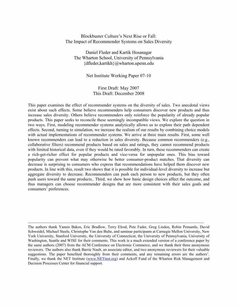
Proposition 2. Relation of limit points to concentration. For any (p,r), the effect on concentration is
Case Support points Effect on concentration relative to p 1 L Increased concentration 2 2 Case 2A: ),( 2
121
rrrp −−
−∈ . Increased concentration for both support points Case 2B: ),( 2
121
rrrp −−
−∉ . Increased concentration for one support point; decreased for the other
3 1 Increased concentration
These cases are shown in Figure 5. For Cases 1 and 3, there is a single outcome and that outcome
always has increased concentration. These are areas of the p×r space where consumers have strong initial
probability (p) relative to the recommender’s strength (r); as a result, the recommender’s effect is to
reinforce this tendency even more. For example, if consumers have a fairly strong tendency to buy w with
p = .90 and the recommender is fairly influential with r = .25, the recommender creates a positive
feedback loop, reinforcing the popularity of w and giving it a limit share of 0.93 > 0.90. Product w was
initially bought more, which made it recommended more, which made it bought more, and so on.
Case 2A occurs where the recommender’s influence (r) is high relative to the initial probability (p).
This has two implications, one at the sample-path and one at the aggregate level. At the sample path level,
either product can win the market, regardless of p. For example, p = 0.55 and r = 0.75 imply limiting
market shares of (w,b) ∈ {(0.89,0.11), (0.14,0.86)}. In the first outcome, w wins the market. In the
second, b wins, even though p = 0.55 initially favored w (c.f. Corollary 1). This occurs because r is large
relative to p, and the recommender reinforces whichever product does well early on without too much
resistance from p. This leads to the finding that recommenders can create hits. Some product will become
a winner with a permanent, majority share, but we cannot say which beforehand. At the aggregate level,
concentration always increases. We do not know which of w or b will win, but we know that one will and
whichever does will be an outcome with greater concentration. Although they start with different models,
a similar phenomenon occurs in other contexts (e.g., studies of firm location). Arthur (1994) provides an
overview of applications, while earlier mathematical results are in Hill (1980).
3 The visual interpretation applies only to where f’s line segments intersect the 45º line (not the single point at Xt = 0.5).
11
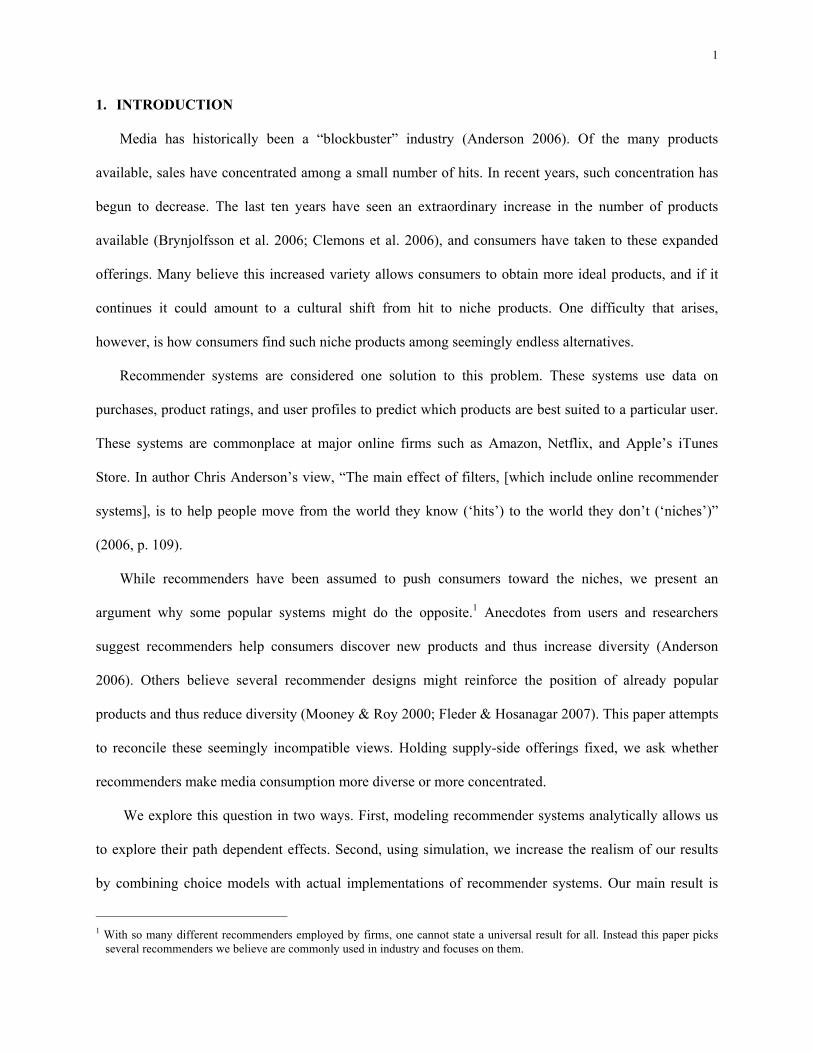
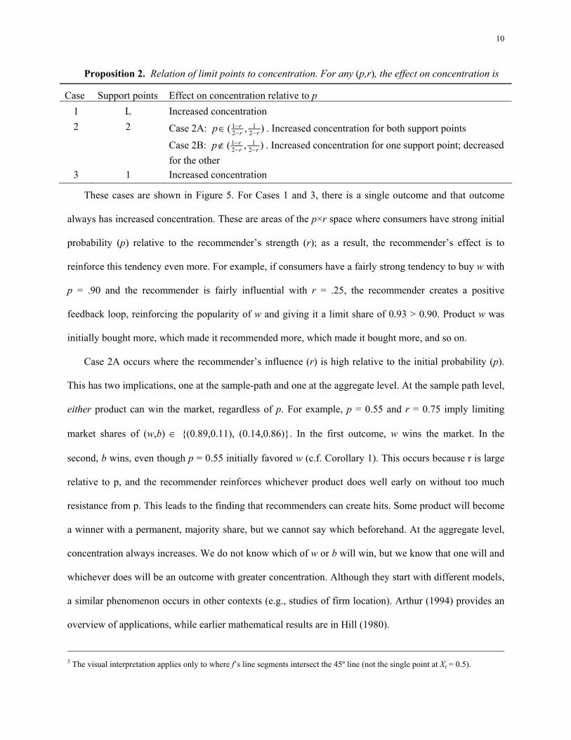
Last, in Case 2B, neither the initial probability (p) nor the recommender’s influence (r) is strong
relative to one another. As a result, two outcomes are possible. The tendency p can be reinforced by the
recommender. This increases concentration. Or, the recommender can give whichever product was not
favored a small majority. This decreases concentration. For example, if p = .60, which is mild, and r =
.25, the limit points are .70 and .45. Often w has more early successes and the recommender reinforces
this, leading to less diverse .70 outcome. In some cases, if b is chosen enough early on, the recommender
reinforces b leading to the .45 outcome, which entails less concentration than the initial share of .40.
0.0 0.5 1.00.0
0.5
1.0
r
p
3
1
2B
2B
2A
0.0 0.5 1.00.0
0.5
1.0
r
p
3
1
2B
2B
2A
Figure 5. Relating the p×r space to concentration effects (numbers refer to cases in Proposition 2).
Figure 6. Concentration increases in white areas and decreases in shaded ones.
While both outcomes are possible in 2B, they are not equally likely. Next we determine the probability of
arriving at each. This, in turn, allows us to calculate the expected effect on concentration.
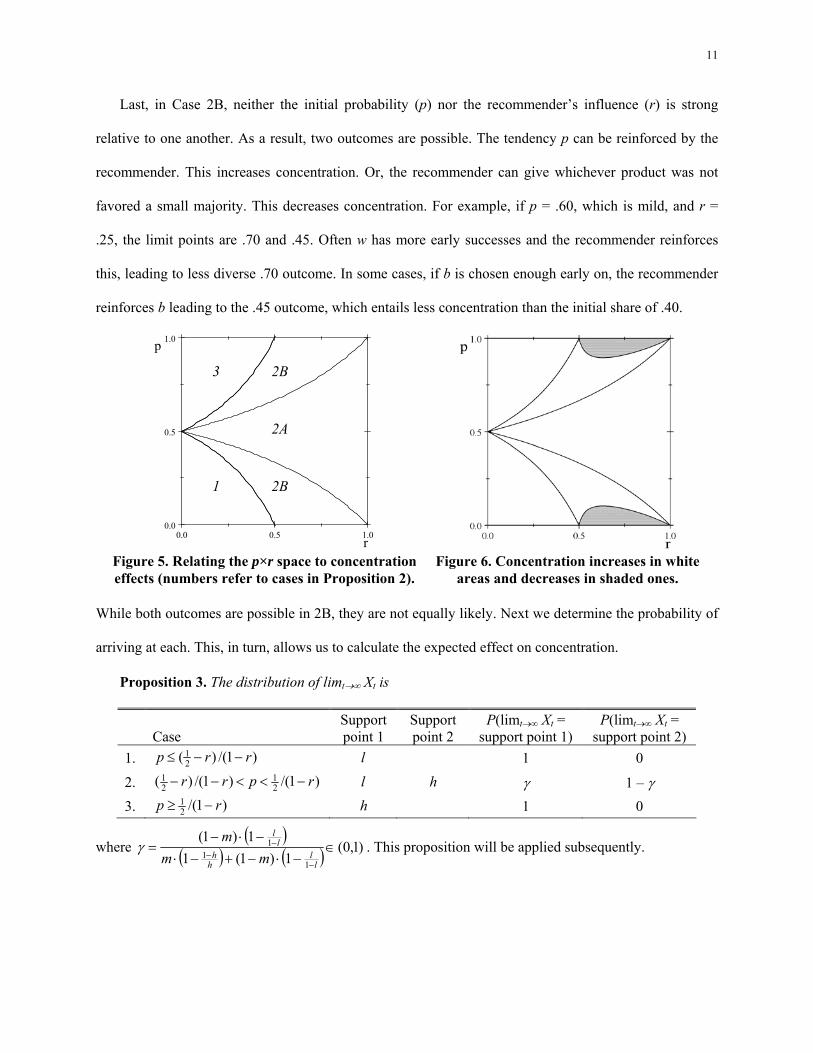
Proposition 3. The distribution of limt→∞ Xt is
Case
Support point 1
Support point 2
P(limt→∞ Xt = support point 1)
P(limt→∞ Xt = support point 2)
1. )1/()( 21 rrp −−≤ l 1 0
2. )1/()1/()( 21
21 rprr −<<−− l h γ 1 – γ
3. )1/(21 rp −≥ h 1 0
where ( )
( ) ( ) )1,0(1)1(1
1)1(
11
1 ∈−⋅−+−⋅
−⋅−=
−−
−
ll
hh
ll
mmm
γ . This proposition will be applied subsequently.
12
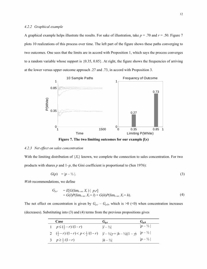
4.2.2 Graphical example
A graphical example helps illustrate the results. For sake of illustration, take p = .70 and r = .50. Figure 7
plots 10 realizations of this process over time. The left part of the figure shows these paths converging to
two outcomes. One sees that the limits are in accord with Proposition 1, which says the process converges
to a random variable whose support is {0.35, 0.85}. At right, the figure shows the frequencies of arriving
at the lower versus upper outcome approach .27 and .73, in accord with Proposition 3.
1 15000
0.35
0.85
110 Sample Paths
Time
P(W
hite
)
0 0.35 0.85 10
1
Limiting P(White)
Frequency of Outcome
0.27
0.73
Figure 7. The two limiting outcomes for our example f(x)
4.2.3 Net effect on sales concentration
With the limiting distribution of {Xt} known, we complete the connection to sales concentration. For two
products with shares p and 1–p, the Gini coefficient is proportional to (Sen 1976):
G(p) = |p – ½ |. (3)
With recommendations, we define
Gp,r = E[G(limt→∞ Xt ) | p,r] = G(l)P(limt→∞ Xt = l) + G(h)P(limt→∞ Xt = h).
(4)
The net effect on concentration is given by Gp,r – Gp,0, which is >0 (<0) when concentration increases
(decreases). Substituting into (3) and (4) terms from the previous propositions gives
Case Gp,r Gp,0 1 )1/()( 2
1 rrp −−≤ |l – ½| |p – ½ |
2 )1/()1/()( 21
21 rprr −<<−− |l – ½|γ + |h – ½|(1 – γ) |p – ½ |
3 )1/(21 rp −≥ |h – ½| |p – ½ |

13
The above gives a closed-form expression for the change in Gini coefficient. Figure 6 shows this
graphically. For most of the p×r square, concentration increases. This is true, of course, for areas under
Case 1, 2A, and 3, where the only possibility was increased concentration. It is also true for most areas
where both outcomes were possible (Case 2B). In extreme cases, it is possible for a net decrease to occur,
as shown by the shading. These areas are largely an artifact of the initial conditions assumed for urn 2,
which place one w and one b in a high r recommender even when p ≈ 0 or ≈ 1. 4
Summarizing, under recommendations the shares converge to either one or two limiting outcomes
depending on (p,r). When there is one outcome, it always reflects increased concentration: the
recommender reinforces the popularity of the initially preferred product. In the two outcome cases, either
both outcomes have greater concentration or one has greater concentration and the other has less. For the
latter, a net effect must be calculated. This typically has greater concentration, although for extreme (p,r),
as discussed, increased diversity may occur. Thus the recommender seems to increase concentration
among a set of similar users.
5. SIMULATIONS
5.1 Rationale for Simulation
Simulation offers three benefits for this problem. First, while actual recommender algorithms are difficult
to represent analytically, they can be implemented in simulation. Second, heterogeneity in user
preferences is easily accommodated. Third, more complex choice processes can be represented.
5.2 Choice Model and Simulation Design
We now turn to a simulation that combines a choice model with actual recommender systems. Repeat
purchases are permitted in the simulation. Examples of contexts with repeat purchases could include
music and video streaming from a subscription service (e.g., Rhapsody).
4 An example illustrates how this is related to initial conditions. Suppose p = 0.99, and r = 0.99, which is in the shaded region.
Since X1 = .50, P(b on first purchase) ≈ 0.50. If b is chosen, the recommender next suggests b; since r = 0.99 the next consumer is almost certain to pick b too, and so on for the remaining consumers even though p = 0.99 favors w. If the initial conditions are determined by k Bernoulli(p) trials, diversity decreases even more: the shaded areas of Figure 6 begin to turn white even for small k. (These additional experiments are available from the authors on request.)
14
An overview of the process is as follows. There are I consumers and J products positioned in an
attribute space. Consumers are not aware of all products. Each consumer knows most of the center
products and a small number of products in his own neighborhood. Every period, a consumer either
purchases one of the products or makes no purchase at all. To model this choice, a multinomial logit is
used for J products plus an outside good. Just before choosing a product, a recommendation is generated.
The recommender has two effects. First, the consumer becomes aware of the recommended product if he
was not already. This increase in awareness is permanent. Second, the salience of the recommended
product is increased temporarily, raising the chance that the recommended product is purchased in that
purchase instance. The next consumer makes a purchase in a similar manner, and the process repeats after
all consumers have purchased. After a predetermined number of iterations, the Gini is computed. The
Gini is then compared to a benchmark G0, the Gini from an equivalent period in which recommendations
were not offered.
We now discuss each of the simulation components: (i) the map of products and consumers, (ii) the
recommender r, (iii) the awareness distribution, (iv) the choice model, and (v) the salience factor δ.
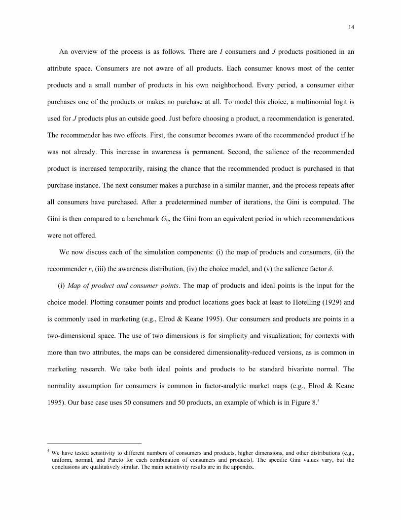
(i) Map of product and consumer points. The map of products and ideal points is the input for the
choice model. Plotting consumer points and product locations goes back at least to Hotelling (1929) and
is commonly used in marketing (e.g., Elrod & Keane 1995). Our consumers and products are points in a
two-dimensional space. The use of two dimensions is for simplicity and visualization; for contexts with
more than two attributes, the maps can be considered dimensionality-reduced versions, as is common in
marketing research. We take both ideal points and products to be standard bivariate normal. The
normality assumption for consumers is common in factor-analytic market maps (e.g., Elrod & Keane
1995). Our base case uses 50 consumers and 50 products, an example of which is in Figure 8.5
5 We have tested sensitivity to different numbers of consumers and products, higher dimensions, and other distributions (e.g.,
uniform, normal, and Pareto for each combination of consumers and products). The specific Gini values vary, but the conclusions are qualitatively similar. The main sensitivity results are in the appendix.
15
Figure 8. Map of product and consumer
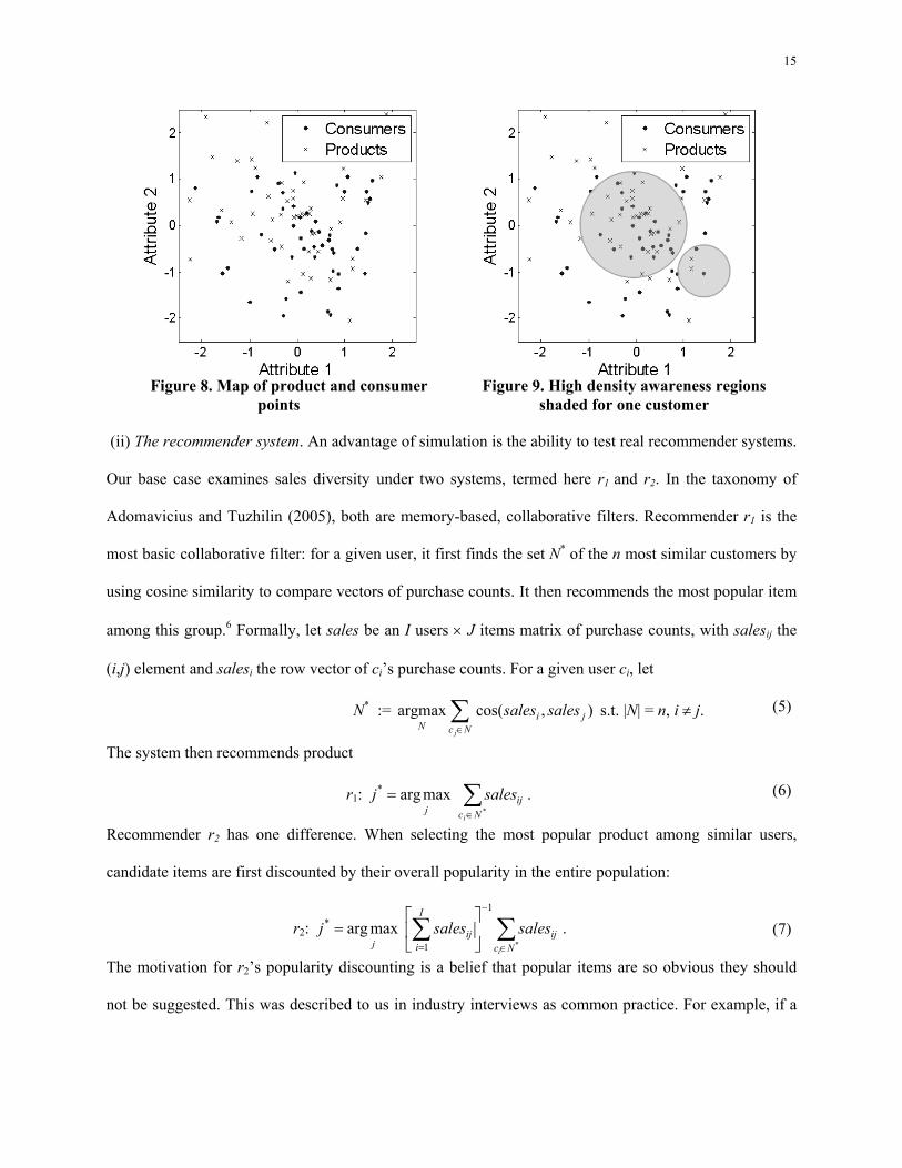
points Figure 9. High density awareness regions
shaded for one customer
(ii) The recommender system. An advantage of simulation is the ability to test real recommender systems.
Our base case examines sales diversity under two systems, termed here r1 and r2. In the taxonomy of
Adomavicius and Tuzhilin (2005), both are memory-based, collaborative filters. Recommender r1 is the
most basic collaborative filter: for a given user, it first finds the set N* of the n most similar customers by
using cosine similarity to compare vectors of purchase counts. It then recommends the most popular item
among this group.6 Formally, let sales be an I users × J items matrix of purchase counts, with salesij the
(i,j) element and salesi the row vector of ci’s purchase counts. For a given user ci, let
N* := ∑∈Nc
jiN
j
salessales ),cos( argmax s.t. |N| = n, i ≠ j. (5)
The system then recommends product
r1: ∑∈
=*
maxarg*
Ncij
ji
salesj . (6)
Recommender r2 has one difference. When selecting the most popular product among similar users,
candidate items are first discounted by their overall popularity in the entire population:
r2: ∑∑
∈
−
=⎥⎦
⎤⎢⎣
⎡=
*
1
1
* maxargNc
ij
I
iij
ji
salessalesj . (7)
The motivation for r2’s popularity discounting is a belief that popular items are so obvious they should
not be suggested. This was described to us in industry interviews as common practice. For example, if a
16
consumer is expected to buy or be aware of a product with high probability, the firm should recommend
something else. Note, r2 is not the same as applying “term-frequency inverse-document frequency”
weights (tf-idf) to algorithm r1. tf-idf would insert discounting in the user similarity calculation (Breese et
al. 1998), whereas r2 inserts it in the final argmax of (7). In Section 7, we test other recommenders,
including one with tf-idf weights, and show the results are directionally the same.
(iii) Awareness. Recommenders are valuable to consumers because they help overcome information
asymmetry: the seller and other users may know of a product, but the given consumer may not.
Recommenders share this information across the population. We assume each consumer is aware of a
subset of the J products, and only items in this awareness set can be purchased. Once an item is
recommended to a consumer, he is always aware of it in future periods. At the start, consumers are aware
of many of the central products on the map plus a few items in their own neighborhood. These initial
awareness states for each consumer-product pair are sampled according to
κθθ λλ /distance/distance 220 )1() of aware ( ijj eepcP ji
−− −+= , (8)
where distance0j and distanceij are respectively the Euclidean distances from the origin to product pj and
from consumer ci to product pj. The higher is λ, the more users are aware of central, mainstream products
(left term), and the higher is 1 – λ the more users are aware of products in their neighborhood. θ and κθ
determine how fast awareness decays with distance. Note that users are not aware of the same products:
they are likely to overlap in their awareness of the central products but less so in the local products.
The awareness model for one consumer is shown in Figure 9 for λ=.75, θ=.35, and κ=1/3. We use
these values for our base case. Setting λ=.75 creates a market with consumers more aware of mainstream
goods than niche ones. This assumption is consistent with a market in which mass advertising makes
consumers aware of the center, mainstream products. Under the opposite (λ < .5), the base-case is already
a market of niches and it only strengthens later results that diversity can decrease. θ determines how many
central products users know. Setting θ=.35 creates an easy to understand “radius 1” rule: e-1/.35 = .057 ≈ 0.
6 An alternative is to use correlation (i.e. cosine on mean-centered data). This does not qualitatively affect the results.

17
In other words, outside a radius of 1, the consumer is unlikely to be aware of the product. In our maps,
about 40% of the products are within 1 unit from the origin; it is on this 40% of products that consumers
are likely to overlap most in their awareness. The value κ determines awareness in the consumer’s own
neighborhood. The value κ=1/3 creates roughly a 0.5 radius rule. Outside the 0.5 radius, the consumer is
unlikely to know about products, unless they are the central ones. The approach in selecting these
parameters was to create an interpretable base case. In sensitivity analysis, we find the Gini can change
for other parameter values but the results are directionally the same.7
(iv) Choice model. At each step of the simulation, a consumer either purchases an item in his
awareness set or makes no purchase at all. We model this using the multinomial logit. The logit is well
established in economics and marketing and has an axiomatic origin in random utility theory (for a
Marketing application, see Guadagni & Little 1983). Consumer ci’s utility for product pj at time t is
defined as uijt := vijt + εijt, where vijt is a deterministic component and εijt is an i.i.d. random variable with
extreme value distribution. Under these assumptions
P(ci buys pj at t | ci aware of pj at t) = ∑ =
J
kv
v
ikt
ijt
e
e
1
. (9)
The unconditional probability is defined P(ci buys pj at t) = P(ci buys pj at t | ci aware of pj at t) P(ci aware
of pj at t). If a consumer is unaware of a product, the rightmost term is zero, and he cannot buy it.
The deterministic component vijt is often modeled as a linear combination of a brand intercept,
product attributes, and covariates (e.g., price, promotion). In our context, since all relevant variables up to
white noise are encompassed in the map, we define the logit’s deterministic portion as
vijt := similarityij = -k log distanceij , (10)
7 If consumers know only the central products (λ=1) the results are directionally the same. If consumers are aware of all products
(θ→∞), the results are the same direction as well. The same holds if awareness is Pareto distributed instead of normal.
18
where distanceij is the Euclidean distance between consumer ci and product pj. Our choice of a log
transformation from distance to similarity is consistent with prior research (e.g., Schweidel et al. 2007).8
The parameter k determines the consumer’s sensitivity to distance on the map. The higher is k, the
more the consumer prefers the closest products. For our base case, as k ranges from 1 to 40, the Gini
increases from .68 to .75. This range is consistent with several prior estimates of market concentration in
media and e-commerce settings. An estimate for a major online clothing retailer is 0.70 (Brynjolfsson et
al. 2007), an estimate for the music sales of debut albums is 0.724 (Hendricks & Sorensen 2007)9, and an
estimate for the online book market is also near 0.75 (Chevalier & Goolsbee 2003)10. To fix a base case,
we use k = 10 because the 0.72 Gini it produces matches the average of the estimates above. This k forms
our base case. For other values, the results change in magnitude but not direction.
Last, as noted, consumers may choose not to purchase. This is modeled by an outside good with equal
distance to all users. This approach is one common specification for modeling a no-purchase option (e.g.,
Chintagunta 2002). Our base cases uses a distance of .75 for this option, which implies the outside good’s
proximity is about 90th percentile (.87) for each consumer. That is, for each person, the outside good is
closer than roughly 90% of the other goods. This means consumers have a fairly good outside option. If
the outside good is farther, consumers substitute farther products for the outside good and diversity
increases. The change in Gini under recommendations, however, is in the same direction.
(v) Salience δ. The term δ is the amount by which a recommended product’s salience is temporarily
increased in the consumer’s choice set. The impact of the salience boost is that the purchase probability
for the recommended item j is the same as that for an item 'j with δ+= ijij vv ' . The functional form is
analogous to the modeling of store displays in marketing (e.g., Guadagni & Little 1983), which might be
8 Other transformations have been used, and the literature does not have a single standard: for example, –k⋅distanceij in Elrod
(1988); (distanceij)-k in DeSarbo and Wu (2001); and -k⋅log(distanceij) in Schweidel et al. (2007) with k a scaling parameter. While our base case uses the log transformation (e.g., Schweidel et al. (2007) and other references contained therein), we have tested sensitivity to the other specifications, and the results are not substantively different.
9 The .724 could underestimate concentration because the authors’ data excludes less successful artists. This may not affect their objective, which differs from that in this paper.

19
considered an offline example of recommendations. The resulting choice probability is P(ci buys pj at t | ci
aware of pj at t) = ( ) 1−
≠+∑ ijtiktijt v
jkvv eeeee δδ .
When δ = 0, the recommender has only an awareness effect. Recommended items enter the awareness
set if not there already. When δ > 0, the recommender also has a salience effect, which increases the
probability of buying the item (conditional on awareness). The salience effect exists for several reasons.
First, consumers aware of many goods may have difficulty comparing all of them; recommended items
become more salient in this comparison. Second, the salience boost may reflect the ease of clicking a
recommended item versus continuing to search through a firm’s website. Last, salience may capture
persuasive effects. Recommendations often show an item’s packaging and artwork, akin to a persuasive
advertisement. We assume the combined effect is to increase the salience by δ. Experiments have begun
to demonstrate that recommendations can have influential effects beyond awareness (Senecal & Nantel
2004). This simultaneity of both effects, awareness and salience, has parallels with advertising’s
informative and persuasive effects (e.g., Narayanan et al. 2005).
The salience term δ is a key parameter because it controls the strength of the recommender. For this
reason, the paper’s main results are shown for a range of δ and not a single point. To give some intuition
for δ, consider the purchase probability of the 75th percentile closest item on the map (with 50 products,
this is the 13th closest item). In our normal maps, if δ = 0 the user chooses item 13 with <10-4 probability.
Item 1 is purchased with probability 0.85. If the 75th percentile item is recommended, for δ = (1, 5, 10,
15) the item takes on purchase probability (<10-3, <.01, .15, and .48) respectively. Thus δ = 0-1 is low, for
it has little effect on purchase probability. A value δ=15 is high, for it makes a close item (100th
percentile) and far item (75th percentile) equal in probability.
10 The Zipf formulation can be equated to a power law, and from the power law a closed form expression for the Gini can be derived. A rank-on-sales coefficient of 1.17 in a power law implies a Gini of (2×1.17 – 1)-1 = 0.75.
20
6. RESULTS
We now present simulation results for the two real-world recommenders.11 We use 50 consumer points
and 50 products sampled from a bivariate normal distribution N2(0,I) with k = 10.
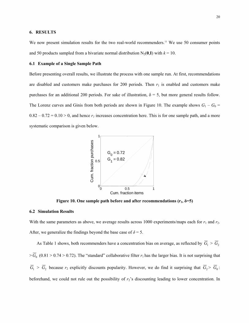
6.1 Example of a Single Sample Path
Before presenting overall results, we illustrate the process with one sample run. At first, recommendations
are disabled and customers make purchases for 200 periods. Then r1 is enabled and customers make
purchases for an additional 200 periods. For sake of illustration, δ = 5, but more general results follow.
The Lorenz curves and Ginis from both periods are shown in Figure 10. The example shows G1 – G0 =
0.82 – 0.72 = 0.10 > 0, and hence r1 increases concentration here. This is for one sample path, and a more
systematic comparison is given below.
0 0.5 10
0.5
1
Cum. fraction items
Cum
. fra
ctio
n pu
rcha
ses
G0 = 0.72
G1 = 0.82
Figure 10. One sample path before and after recommendations (r1, δ=5)
6.2 Simulation Results
With the same parameters as above, we average results across 1000 experiments/maps each for r1 and r2.
After, we generalize the findings beyond the base case of δ = 5.
As Table 1 shows, both recommenders have a concentration bias on average, as reflected by 1G > 2G
> 0G (0.81 > 0.74 > 0.72). The “standard” collaborative filter r1 has the larger bias. It is not surprising that
1G > 2G because r2 explicitly discounts popularity. However, we do find it surprising that 2G > 0G :
beforehand, we could not rule out the possibility of r2’s discounting leading to lower concentration. In

21
fact, in a small number of runs (17%), r2 increases diversity, but in the majority of runs (83%) and on
average it reduces diversity. A t-test of paired differences for unequal means (pre versus post
recommendations) shows the differences are significant.
For r1, this is partly explained by (6), in which popularity determines what product is recommended.
This creates a self-reinforcing cycle: popular items are recommended more, items recommended more are
purchased more, purchased items are recommended more, and so on. Despite this, the increased
concentration was not readily obvious: recommendations are generated in many local user groups, making
a priori conclusions difficult. Although r2 dampens the popularity bias, the result also originates from
using only sales data to make recommendations. Products with limited historical sales have little or no
chance of being recommended even if they would be favorably received by the consumer.12
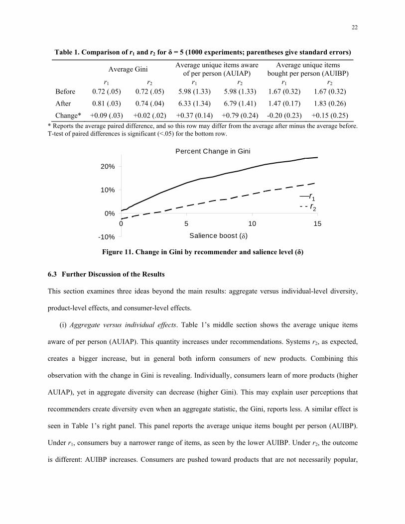
Figure 11 shows the change in Gini for a range of δ. When the recommender has both awareness and
salience effects, concentration increases in δ. The effect is most pronounced at high δ, where by
construction the recommender has a bigger effect. In the special case δ = 0, the recommender has only
awareness effects. System r1 continues to increase concentration, although by much less (+1.4%), as seen
in Figure 11. The feedback loop is weaker: even if popular items are recommended more, recommended
items are not necessarily purchased more because δ = 0. As a result, the Gini’s increase is attenuated.
With r2, diversity increases under δ = 0, although the magnitude is small (-1.4%) as shown in Figure 11.
The deliberate exploration of r2 coupled with low salience of recommendations increases diversity.
To summarize, when recommenders have both effects, diversity generally decreases. When
recommenders affect only awareness, diversity decreases slightly for r1 and increases slightly for r2. The δ
= 0 case is of conceptual interest, although it may not be commonplace. It is difficult to show consumers
information without influencing them. As an example, the experiments of Senecal and Nantel (2004)
show recommendations are influential even when consumers are aware of all products.
11 The simulation code is available from the authors upon request 12 With content based recommenders, we would not expect the same dynamics because past sales no longer affect which product
is recommended. Studying the diversity question for content based systems is an interesting question but beyond the current scope.
22
Table 1. Comparison of r1 and r2 for δ = 5 (1000 experiments; parentheses give standard errors)
Average Gini Average unique items aware of per person (AUIAP)
Average unique items bought per person (AUIBP)
r1 r2 r1 r2 r1 r2 Before 0.72 (.05) 0.72 (.05) 5.98 (1.33) 5.98 (1.33) 1.67 (0.32) 1.67 (0.32)
After 0.81 (.03) 0.74 (.04) 6.33 (1.34) 6.79 (1.41) 1.47 (0.17) 1.83 (0.26)
Change* +0.09 (.03) +0.02 (.02) +0.37 (0.14) +0.79 (0.24) -0.20 (0.23) +0.15 (0.25) * Reports the average paired difference, and so this row may differ from the average after minus the average before. T-test of paired differences is significant (<.05) for the bottom row.
Percent Change in Gini
-10%
0%
10%
20%
0 5 10 15
Salience boost (δ)
––r1- - r2
Percent Change in Gini
-10%
0%
10%
20%
0 5 10 15
Salience boost (δ)
––r1- - r2
Figure 11. Change in Gini by recommender and salience level (δ)
6.3 Further Discussion of the Results
This section examines three ideas beyond the main results: aggregate versus individual-level diversity,
product-level effects, and consumer-level effects.
(i) Aggregate versus individual effects. Table 1’s middle section shows the average unique items
aware of per person (AUIAP). This quantity increases under recommendations. Systems r2, as expected,
creates a bigger increase, but in general both inform consumers of new products. Combining this
observation with the change in Gini is revealing. Individually, consumers learn of more products (higher
AUIAP), yet in aggregate diversity can decrease (higher Gini). This may explain user perceptions that
recommenders create diversity even when an aggregate statistic, the Gini, reports less. A similar effect is
seen in Table 1’s right panel. This panel reports the average unique items bought per person (AUIBP).
Under r1, consumers buy a narrower range of items, as seen by the lower AUIBP. Under r2, the outcome
is different: AUIBP increases. Consumers are pushed toward products that are not necessarily popular,
23
which means they are less likely to have bought them previously. The Gini, however, still increases. This
again leads to the finding that individual diversity can increase while aggregate diversity decreases.
Consumers are discovering new products, but they are discovering the same products others have bought.
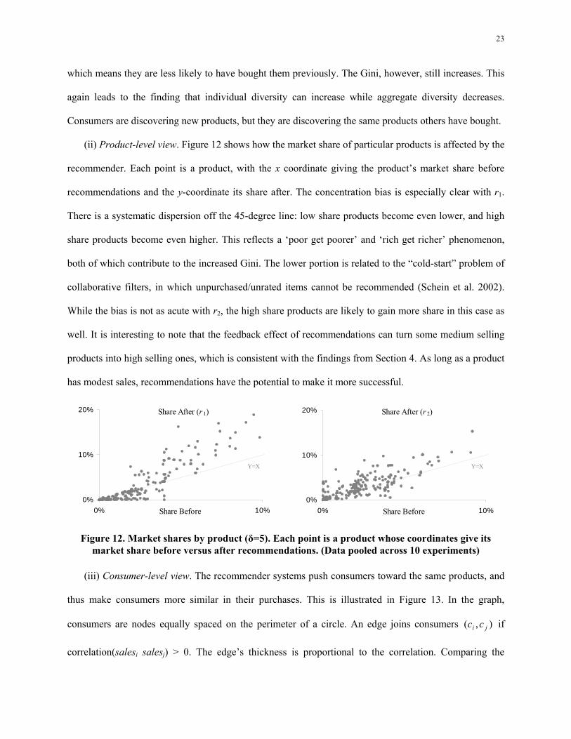
(ii) Product-level view. Figure 12 shows how the market share of particular products is affected by the
recommender. Each point is a product, with the x coordinate giving the product’s market share before
recommendations and the y-coordinate its share after. The concentration bias is especially clear with r1.
There is a systematic dispersion off the 45-degree line: low share products become even lower, and high
share products become even higher. This reflects a ‘poor get poorer’ and ‘rich get richer’ phenomenon,
both of which contribute to the increased Gini. The lower portion is related to the “cold-start” problem of
collaborative filters, in which unpurchased/unrated items cannot be recommended (Schein et al. 2002).
While the bias is not as acute with r2, the high share products are likely to gain more share in this case as
well. It is interesting to note that the feedback effect of recommendations can turn some medium selling
products into high selling ones, which is consistent with the findings from Section 4. As long as a product
has modest sales, recommendations have the potential to make it more successful.
Share After (r 1)
0%
10%
20%
0% 10%Share Before
Y=X
Share After (r 2)
0%
10%
20%
0% 10%Share Before
Y=X
Figure 12. Market shares by product (δ=5). Each point is a product whose coordinates give its market share before versus after recommendations. (Data pooled across 10 experiments)
(iii) Consumer-level view. The recommender systems push consumers toward the same products, and
thus make consumers more similar in their purchases. This is illustrated in Figure 13. In the graph,
consumers are nodes equally spaced on the perimeter of a circle. An edge joins consumers ),( ji cc if
correlation(salesi salesj) > 0. The edge’s thickness is proportional to the correlation. Comparing the

24
graphs, the increased density at right shows that consumers have become more similar in their purchases.
The figure alone does not imply the Gini has increased. For example, a correlation of 1 among all users
could occur if everyone bought a single product (Gini=1), but it could also occur if all users bought all
items equally (Gini=0). On its own, the figure shows consumers have become more alike. Combining this
with the increased Gini, we see the complete picture: users are more similar (from Figure 13), and the
items they purchase come from a smaller, more popular set (Ginis in Table 1).
Before Recommendations After Recommendations
Figure 13. Each point is a user, and edge thickness is proportional to the pair’s similarity
7. SENSITIVITY ANALYSIS
We approach sensitivity analysis in four parts: additional recommenders; best-seller lists in the base case;
variety seeking in the utility specification, and alternate parameter values.
7.1 Alternate Recommender Systems
The base case examined two recommenders that were considered representative of industry practice. This
section tests additional systems. A comparison of eight recommenders ri (i=1,...,8) is given in Table 2.
The recommenders tested are as follows. r1 and r2 are as before. r3 is another popularity-discounting
variation on r1 (Breese et al. 1998). It places discounting in the user similarity calculation but not the
product selection calculation. (i.e. r2 and r3 add discounting in opposite places). Specifically, in (5) the
user-item frequencies are multiplied by the inverse of each item’s total sales (known as the “inverse
document frequency” (idf) in the field of information retrieval); once the similar user group is determined,
the undiscounted argmax of (6) is used. This still leads to an increase in the Gini. The magnitude is
similar to r1’s increase for the following reason. The intention of r3 is to prevent latently different users

25
with little purchase history from being grouped together (e.g., two users who each bought Harry Potter
and one very different item). Because of the initialization period, our users have several purchases, and so
the similar user-groups under r1 and r3 are often similar (and hence 1G ≈ 3G ). System r4 is a combination
of r2 and r3: discounting is performed in both the user similarity calculation and argmax. As with its
parents, r4 also lowers diversity.
To build context for these comparisons, we tested four other designs (r5 – r8). System r5 recommends
the lowest sales product. As expected, it decreases the Gini. System r6 recommends the median selling
product. It also reduces the Gini because it diverts attention from otherwise higher selling products.
System r7 recommends the best-selling product and as expected increases the Gini. We highlight that the
Gini under r7 is not higher than under r1. A single product, the best seller, cannot be close to everyone.
As a result, fewer users accept r7’s recommendations, limiting its influence. In contrast, r1 recommends
local best-sellers, which are closer to each user and thus accepted more. r8 is a best-seller list, which
recommends the top 5 selling items. This system has the highest concentration: it shows the most popular
items, and by showing multiple items increases the chance that at least one is close to the user. Similar
results were confirmed experimentally by Salganik et al. (2006).
Table 2. Comparison of additional recommenders (1000 experiments).
r1 r2 r3 (r1 + idf weights) r4 (r2 + r3 combined)
iG 0.81 (0.03) 0.74 (0.05) 0.81 (0.03) 0.74 (0.05)
0GGi −* +0.09 (0.03) +0.02 (0.02) +0.09 (0.03) +0.02 (0.02)
r5 (lowest) r6 (median) r7 (highest) r8 (top-five sellers) iG 0.45 (0.10) 0.61 (0.03) 0.81 (0.04) 0.85 (0.03)
0GGi −* -0.27 (0.10) -0.11 (0.04) +0.09 (0.02) +0.14 (0.04)
* Significant at the 0.05 level (2-sided, paired differences t-test for unequal means). For all cases, 0G = 0.72 (0.05). 7.2 Best-seller Lists in the Base Case
Without recommenders, consumers might obtain product suggestions from best-seller lists. We model
this by introducing a best-seller list in the base case. This is equivalent to r8 from the previous subsection
– but now r8 is the base case and r1 or r2 the treatment. Viewed this way (Table 2), the Gini decreases:

26
1G < 8G (0.82 < 0.85) and 2G < 8G (0.75 < 0.85). If recommenders are simply replacements for best-
seller lists, diversity can increase by cutting out what is an even more popularity-biased tool. Although it
is unlikely that best-seller lists drive purchase decisions in all product categories, it seems feasible that
best-seller lists affect purchase decisions in some categories. If so, this implies the role of recommenders
is misunderstood. Relative to an ‘older’ world of best-seller lists, recommenders may reduce
concentration, by virtue of cutting out the even more popularity-biased tool ( 1G , 2G < 8G ). But relative to
a world without such lists, recommenders may increase concentration ( 1G , 2G > 0G ).
7.3 Modifying the Utility Specification: Variety Seeking
Since the choice model allowed for repeat purchases, we ask whether the concentration results are
affected if consumers seek variety across purchase occasions. The concept of state dependence has a long
history in choice models (e.g., McAlister 1982). “Structural state dependence” (Seetharaman 2004) is the
extent to which prior purchases of a product affect its future purchase propensity; positive dependence is
termed inertia, while negative dependence is termed variety seeking.
To incorporate variety and inertia in the specification, we use a common approach and define
vijt := -k log distanceij + βXijt
Xijt := αXijt-1 + (1 – α)I(ci bought pj on t – 1).
Xijt is an exponential smooth of purchase indicators I( ), and thus it summarizes how often and recently ci
has bought pj. The parameter α ∈ (0,1) determines how much weight is placed on recent versus distant
purchase occasions. β determines the effect strength, with β < 0 for variety seeking, and β > 0 for intertia.
This approach has been used frequently in the literature (e.g., see Guadagni & Little 1983; Seetharaman
2004). Past empirical studies have found consistent values of α in the range 0.70-0.80, and thus we set α
= 0.75 (Guadagni & Little 1983; Lattin 1987; Seetharaman 2004). For β, we consider a range of values to
explore both variety-seeking and inertia. The β term is not applied to the outside good, which by
definition has the same distance to all consumers at all times.

27
Table 3 shows the Gini under state dependence. Under inertia (β > 0), the findings are directionally
the same as before: concentration increases. Under high inertia, consumers do not want to deviate from
their choices in the pre-recommendation period, and so the recommender’s influence becomes limited.
Under variety seeking (β < 0), concentration still increases for r1 but by less. r1 suggests heavily
purchased items, which are less likely to provide variety. As a result, users ignore recommendations that
are too similar, and the change in Gini is lessened. For r2, at moderate levels of variety seeking (e.g., β = -
5) concentration still increases. At strong levels of variety seeking, the diversity can increase. For
example, at β = -20, the Gini drops .03 points. We note that this level of variety seeking is high. Suppose
ci buys pj semi-frequently so that Xijt = 0.5 at some time. β = -20 implies βXijt = (-20)(0.5) = -10, which is
twice as strong as the δ = 5 salience effect of recommendations. Under such high variety seeking, the Gini
decreases because users ignore recommendations of popular items and selectively accept
recommendations of less popular ones. Whereas r1 cannot supply these (r1 focuses on past hits), r2 makes
this possible. Users want items not purchased recently, and r2’s discounting meets this goal.13
The variety seeking results have an interesting interpretation. If consumers turn to recommendations
only in their most variety-seeking moments, diversity increases under r2. However, as recommenders
become ubiquitous, consumers are affected by them all the time – e.g., as with sites users visit regularly,
such as personalized news, personalized radio, and personalized retail. In these instances, diversity
decreases even under r2.
Table 3. Gini values under state dependence at δ=5. For variety seeking β < 0, and for inertia β > 0
β -30 -20 -10 -5 0 5 10 20 30
01 GG − +.04 +.05 +.07 +.08 +.09 +.07 +.04 +.02 +.02
02 GG − -.04 -.03 -.01 +.01 +.02 +.03 +.02 +.02 +.02
13 Letting variety seeking go to –∞, we test the case where repeat purchases are not allowed. To implement this, we ensure the
number of products is more than the number of simulation iterations. The results are similar to those in Table 3. Concentration still increases under r1. Consumers always buy new products, but the recommender still pushes them toward products that others purchased previously. With r2, concentration can decrease at such a high level of variety seeking as discussed above.

28
7.4 Altering Other Simulation Parameters
We also examine sensitivity to other simulation parameters (e.g., number of consumers and products, map
distributions). The main sensitivity results appear in the online appendix, and others are available on
request. In general, we find that varying these parameters affects the degree of the results (e.g., the Gini
may increase more versus less), but the substantive findings remain the same.
8. WELFARE IMPLICATIONS
Thus far we have examined how recommenders affect concentration. We next ask whether these changes
leave firms and consumers better off.
For firms, we examine the change in sales. For consumers, we examine the change in product fit.
Consumers’ product fit is defined as the average of -k log distanceij + εijt over all purchases, including
those of the outside good. This measure reflects the map distance between consumers and purchased
products. Figure 14 shows these quantities, plotting the numbers in percent change so that both firm and
consumer effects can be plotted together. When δ = 0, the recommender has a pure awareness effect. The
firm’s sales are higher, and consumers find products closer to them. The gains for both parties are larger
under r2. The deliberate exploration of r2 helps consumers find better products, which translates into
higher sales (fewer no-purchases) for the firm. When δ > 0, recommenders have both awareness and
salience effects. At low δ, the results are the same as δ = 0. At high δ, firms always sell more: the greater
the salience δ, the more likely the consumer is to buy the recommended product than the outside good.
For consumers, high δ increases the average map distance of purchases: consumers may forgo a slightly
closer product if the recommended product has increased salience. A slightly better song or news article
may be available deeper in the website, but the recommendation’s salience makes it easier to click.
Does this mean consumers are worse off if δ >> 0? If the salience effect is simply a momentary
increase in purchase probability but does not contribute to post-purchase satisfaction, then consumers are
worse off because their purchases are farther away. However, a more complete answer considers
additional factors. First, it is possible that δ, or part of it, should be included in the consumer’s utility.

29
This is the case if recommendations add value to the choice occasion. In this case, the consumer effect in
Figure 14 becomes positive and increasing (not shown for clarity). This view is consistent with several
logit applications in marketing in which a store display adds utility to the choice occasion (e.g., Guadagni
& Little 1983). For example, a display means the user does not have to walk down the aisle to get the
product or price information. Similarly, choosing the recommended item may
Percent Change
-10%
0%
10%
20%
30%
0 5
Salience boost (δ)
––r1- - r2
Sales
– k·log(distance)+ε
Percent Change
-10%
0%
10%
20%
30%
0 5
Salience boost (δ)
––r1- - r2
Sales
– k·log(distance)+ε
Figure 14. Percent changes in consumer and producer surplus for varying levels of salience (δ) save time browsing the site or effort in making product comparisons. Second, to the extent media
products have positive externalities, these may offset the increased distance. For example, watching the
same movies as others is valuable if it permits discussion. In this case, the recommender serves a
coordinating role whose value is not fully accounted for by measuring map distances. For firms, we
measured the change in sales. To the extent changes in concentration simplify inventory management,
these factors are also unaccounted for. Last, recommenders may have welfare implications at the societal
level. Sunstein (2001) discusses the risk of “filters” creating a fragmented society. He asks whether en
masse filtering of all but one's exact interests will reduce people’s ability to understand one another. Such
considerations are beyond the current scope, but we raise them to show that an exhaustive analysis of
welfare implications would involve more than changes in sales and map distances.
9. CONCLUSIONS AND FUTURE WORK
This paper examined the effect of popular recommender designs on sales concentration and offered
evidence that recommenders do influence sales diversity. Several common recommenders were found to
30
exert a concentration bias. Thus the traditional view that recommenders increase diversity may not always
hold. The work also demonstrated that some designs may be associated with greater bias than others. The
results have important managerial and consumer implications. We find that recommenders can increase
sales, and recommenders that discount popularity appropriately may increase sales more. For consumers,
we showed that the awareness effects of recommenders can inform consumers of better (closer) products.
However, if recommendations are highly salient, popularity-influenced recommendations may displace
what would otherwise be better product matches. Future, empirical work would be valuable for
determining the relative strength of the awareness versus salience effects.
Given these findings, why do consumers feel that recommendations have increased the range of
media they consume? We offered several explanations. The first is that diversity can increase at the
individual level but still decrease in aggregate. This was borne out under r2, in which each user became
aware of more items and purchased more unique items, but the Gini still increased. Individuals may be
exploring more choices, but they are being pushed toward the same choices. Second, if recommenders are
simply replacing best-seller lists, diversity can increase by virtue of cutting out an even more popularity-
biased tool. A final possibility is that the effect of increased product offerings outweighs the effect of
recommenders. Increased offerings may lower concentration (Anderson 2006; Brynjolfsson et al. 2007),
while recommenders could temper but not reverse the effect. Examining the simultaneous effects of
recommenders and increased offerings is an interesting question for future work.
A final interesting aspect arose to the extent that externalities exist for media goods. If, for example,
there is a benefit to reading popular books or seeing popular movies (e.g., by increasing the likelihood of
being able to discuss the experience with others), then consumer utility involves a tradeoff between a
Hotelling-like similarity and the externality from a popular product. To the extent such externalities are
strong, it would be interesting to see if they pose a limit, or upper bound, on the degree of diversity
consumers would ever prefer. If this were the case, a concentration bias may be more desirable than
previously considered. We hope to explore these questions in future work as well.
31
10. REFERENCES
Adomavicius, G. and A. Tuzhilin. 2005. Toward the next generation of recommender systems: a survey of the state-of-the-art and possible extensions. IEEE Trans. Know. Data. Eng. 17(6):734-749. Anderson, C. 2006. The Long Tail. New York: Hyperion. Ansari, A., S. Essegaier, and R. Kohli. 2000. Internet recommendation systems. J. Mktg.Res. 37(3):363-375. Arthur, W. B. 1994. Increasing Returns and Path Dependence in the Economy. Ann Arbor: University of Michigan Press. Bikhchandani, S., D. Hirshleifer, and I. Welch. 1998. Learning from the behavior of others: conformity, fads, and informational cascades. J. of Economic Perspectives 12:3 151-170. Bodapati, A. 2008. Recommendation systems with purchase data. J. Mktg. Res. 45(1):77-93. Breese, J., D. Heckerman, and C. Kadie. 1998. Empirical analysis of predictive algorithms for collaborative filtering. In Proc. of the 14th Conference of Uncertainty in AI. Brynjolfsson, E., Y. Hu, and D. Simester. 2007. Goodbye Pareto principle, hello long tail: the effect of search costs on the concentration of product sales. SSRN eLibrary 953587. Brynjolfsson, E., Y. Hu, and M. Smith. 2006. From niches to riches: the anatomy of the long tail. Sloan Management Review 47(4) 67-71. Chevalier, J. and A. Goolsbee. 2003. Measuring prices and price competition online: Amazon.com and BarnesandNoble.com. Quantitative Marketing and Economics 1(2):203-222. Chintagunta, P. 2002. Investigating category pricing behavior at a retail chain. J. Mktg. Res. 39(2):141-54 Clemons, E.K., G. G. Gao, and L.M. Hitt. 2006. When online reviews meet hyperdifferentiation. J. of Management Information Systems 23(2):149-171. Cooke, A., H. Sujan, M. Sujan, and B. Weitz. 2002. Marketing the unfamiliar: the role of context and item-specific information in electronic agent recommendations. J. Mktg. Res. 39(4):488-497. DeSarbo, W. S. and J. Wu. 2001. The joint spatial representation of multiple variable batteries collected in marketing research. Journal of Marketing Research 38(2):244-253. Elrod, T. and M. P. Keane. 1995. A factor-analytic probit model for representing the market structure in panel data. J. of Marketing Research 32(1):1-16. Fleder, D. and K. Hosanagar. 2007. Recommender systems and their impact on sales diversity. In Proc. of the 8th ACM Conference on Electronic Commerce, p. 192-199. Guadagni, P.M. and J.D.C. Little. 1983. A logit model of brand choice calibrated on scanner data. Marketing Science 2(3):203-238.
32
Hendricks, K. and A. T. Sorensen. 2007. Information spillovers in the market for recorded music. NBER working paper W12263. Last accessed 02/18/08 at <www.stanford.edu/~asorense>. Hill, B. M., D. Lane, and W. Sudderth. 1980. A strong law for some generalized urn processes. Annals of Probability 8(2):214-226. Hotelling, H. 1929. Stability in competition. The Economic Journal 39:41-57. Lattin, J. M. 1987. A model of balanced choice behavior. Marketing Science 6(1):48-65. Linden, G., B. Smith, and J. York. 2003. Amazon.com recommendations: item-to-item collaborative filtering. IEEE Internet Computing 7(1):76-80. McAlister, L. 1982. A dynamic attribute satiation model for choices made across time. J. Cons. Res. 9(3):141-150. Mooney, R. J. and L. Roy. 2000. Content-based book recommending using learning for text categorization. 5th ACM Conf. on Digital Libraries, p.195-204. Narayanan, S., P. Manchanda, and P. K. Chintagunta. 2005. Temporal differences in the role of marketing communication in new product categories. J Mktg. Res. 42(3):278-290. Resnick, P. and H. Varian. 1997. Recommender systems. Comm. of the ACM 40(3):56-58. Salganik, M. J., P. S. Dodds, and D. J. Watts. 2006. Experimental study of inequality and unpredictability in an artificial cultural market. Science 311(5762):854-856. Schafer, J., J. Konstan, and J. Riedl. 1999. Recommender systems in e-commerce. ACM EC, p.158-166. Schein A. I., A. Popescul, L. H. Ungar, and D. M. Pennock. 2002. Methods and metrics for cold- start recommendations. SIGIR, p. 253-260. Schweidel, D. A., E. Bradlow, and P. Fader. 2007. Modeling the evolution of customers' service portfolios. SSRN eLibrary 985639 Seetharaman, P. B. 2004. Modeling multiple sources of state dependence in random utility models: a distributed lag approach. Marketing Science 23(2):263-271. Sen, A. 1976. Poverty: an ordinal approach to measurement. Econometrica 44(2):219-231. Senecal, S. and J. Nantel. 2004. The influence of online product recommendations on consumers’ online choices. Journal of Retailing 80:159-169. Sunstein, C. R. 2001. Republic.com. Princeton: Princeton University Press. Van Alstyne, M. and E. Brynjolfsson. 2005. Global village or cyber-Balkans? Modeling and measuring the integration of electronic communities. Management Science 51(6):851-868.
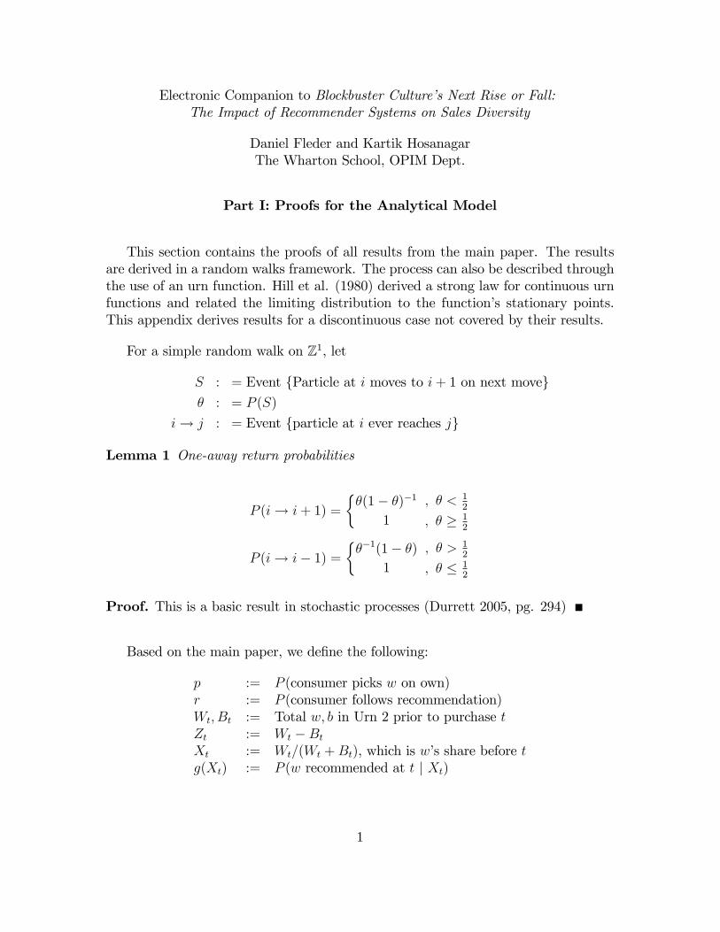
Electronic Companion to Blockbuster Culture�s Next Rise or Fall:The Impact of Recommender Systems on Sales Diversity
Daniel Fleder and Kartik HosanagarThe Wharton School, OPIM Dept.
Part I: Proofs for the Analytical Model
This section contains the proofs of all results from the main paper. The resultsare derived in a random walks framework. The process can also be described throughthe use of an urn function. Hill et al. (1980) derived a strong law for continuous urnfunctions and related the limiting distribution to the function�s stationary points.This appendix derives results for a discontinuous case not covered by their results.
For a simple random walk on Z1, let
S : = Event {Particle at i moves to i+ 1 on next move}
� : = P (S)
i! j : = Event {particle at i ever reaches j}
Lemma 1 One-away return probabilities
P (i! i+ 1) =
��(1� �)�1
1
; � < 12
; � � 12
P (i! i� 1) =���1(1� �)
1
; � > 12
; � � 12
Proof. This is a basic result in stochastic processes (Durrett 2005, pg. 294)
Based on the main paper, we de�ne the following:
p := P (consumer picks w on own)r := P (consumer follows recommendation)Wt; Bt := Total w; b in Urn 2 prior to purchase tZt := Wt �BtXt := Wt=(Wt +Bt), which is w�s share before tg(Xt) := P (w recommended at t j Xt)
1

The chance a consumer selects w at t is
f(Xt) := P (consumer buys w at tjXt)
= p(1� r) + g(Xt)r
The function f is known as an urn function (Hill et al. 1980). It maps the unitinterval into itself and de�nes a process that is Markov but can have nonstationarytransition probabilities.
As de�ned in the paper, g is the step function
g(Xt) :=
8<:0 ; Xt <
12
12; Xt =
12
1 ; Xt >12
This choice of g recommends the product with majority share.
Substituting g(Xt) into f(Xt) gives
f(Xt) =
8<:p(1� r); Xt <
12
"l"p(1� r) + r=2; Xt =
12
"m"p(1� r) + r; Xt >
12
"h"
The letters l, m, h are shorthand for the expressions at their left. They also havea geometric interpretation: f is a modi�ed step function (shifted and stretched), andl, m, and h correspond to the height of f�s lower segment, middle point, and uppersegment respectively. This interpretation was shown graphically in the main paper.
While the main paper states results about fXtg, we can equivalently study fZtg:studying sales instead of shares carries the same information because Xt is a statisticof sales. This switch, however, is bene�cial because Zt changes by one unit eachperiod and so is ammenable to a random walks framework.
For any time � at which Z� = 0 (i.e. W� = B� ), three events are possible
WB := EventfZt > 0 for all t > � jZt = 0gBW := EventfZt < 0 for all t > � jZt = 0gRTZ := EventfZt = 0 for some t > � jZt = 0g
In words, WB is the event that w leads b forever after the next time step; BW isthe event that b leads w forever after the next time step; and RTZ is the event thatZt returns to zero at some future time point.
We now have a random walk on Z1 beginning at the origin for which the transitionprobabilities of moving left versus right are (l; 1 � l); (m; 1 � m), and (h; 1 � h)depending on whether the particle is left of zero, at zero, or right of zero.
2
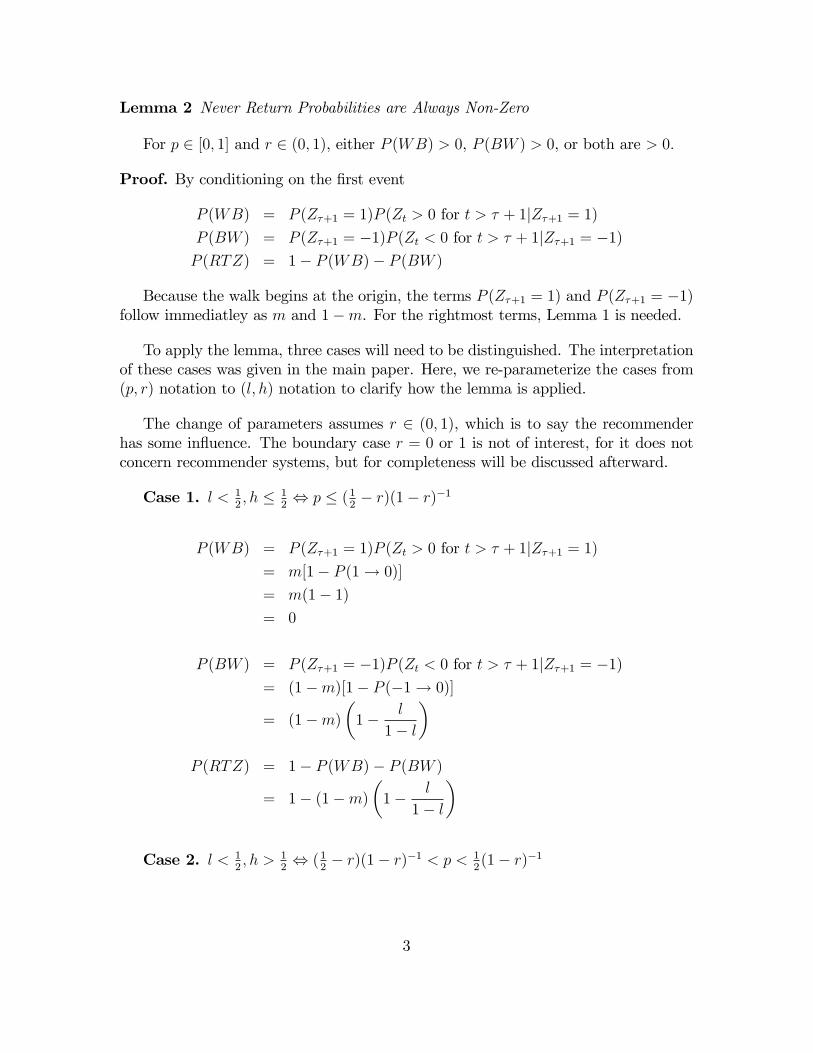
Lemma 2 Never Return Probabilities are Always Non-Zero
For p 2 [0; 1] and r 2 (0; 1), either P (WB) > 0, P (BW ) > 0, or both are > 0:
Proof. By conditioning on the �rst event
P (WB) = P (Z�+1 = 1)P (Zt > 0 for t > � + 1jZ�+1 = 1)P (BW ) = P (Z�+1 = �1)P (Zt < 0 for t > � + 1jZ�+1 = �1)P (RTZ) = 1� P (WB)� P (BW )
Because the walk begins at the origin, the terms P (Z�+1 = 1) and P (Z�+1 = �1)follow immediatley as m and 1�m. For the rightmost terms, Lemma 1 is needed.
To apply the lemma, three cases will need to be distinguished. The interpretationof these cases was given in the main paper. Here, we re-parameterize the cases from(p; r) notation to (l; h) notation to clarify how the lemma is applied.
The change of parameters assumes r 2 (0; 1), which is to say the recommenderhas some in�uence. The boundary case r = 0 or 1 is not of interest, for it does notconcern recommender systems, but for completeness will be discussed afterward.
Case 1. l < 12; h � 1
2, p � (1
2� r)(1� r)�1
P (WB) = P (Z�+1 = 1)P (Zt > 0 for t > � + 1jZ�+1 = 1)= m[1� P (1! 0)]
= m(1� 1)= 0
P (BW ) = P (Z�+1 = �1)P (Zt < 0 for t > � + 1jZ�+1 = �1)= (1�m)[1� P (�1! 0)]
= (1�m)�1� l
1� l
�P (RTZ) = 1� P (WB)� P (BW )
= 1� (1�m)�1� l
1� l
�
Case 2. l < 12; h > 1
2, (1
2� r)(1� r)�1 < p < 1
2(1� r)�1
3
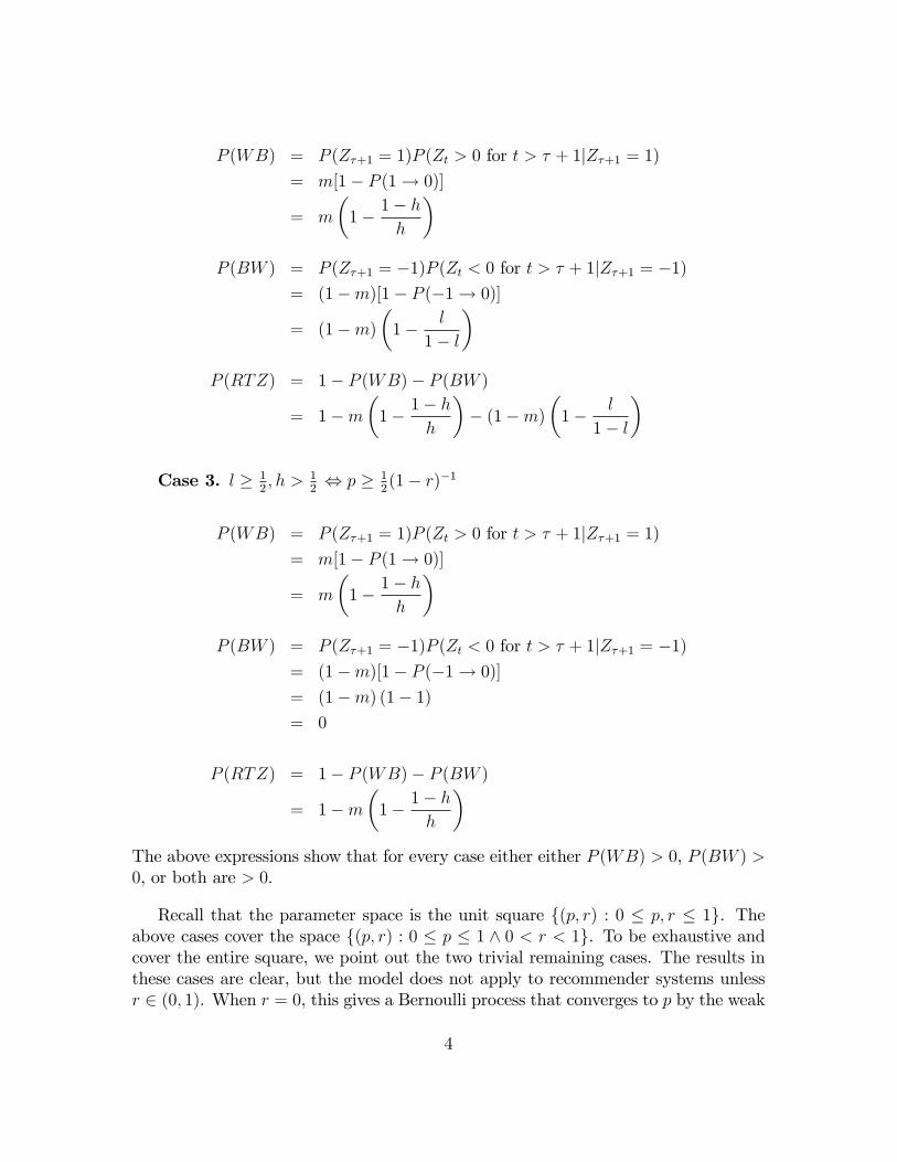
P (WB) = P (Z�+1 = 1)P (Zt > 0 for t > � + 1jZ�+1 = 1)= m[1� P (1! 0)]
= m
�1� 1� h
h
�P (BW ) = P (Z�+1 = �1)P (Zt < 0 for t > � + 1jZ�+1 = �1)
= (1�m)[1� P (�1! 0)]
= (1�m)�1� l
1� l
�P (RTZ) = 1� P (WB)� P (BW )
= 1�m�1� 1� h
h
�� (1�m)
�1� l
1� l
�
Case 3. l � 12; h > 1
2, p � 1
2(1� r)�1
P (WB) = P (Z�+1 = 1)P (Zt > 0 for t > � + 1jZ�+1 = 1)= m[1� P (1! 0)]
= m
�1� 1� h
h
�P (BW ) = P (Z�+1 = �1)P (Zt < 0 for t > � + 1jZ�+1 = �1)
= (1�m)[1� P (�1! 0)]
= (1�m) (1� 1)= 0
P (RTZ) = 1� P (WB)� P (BW )
= 1�m�1� 1� h
h
�The above expressions show that for every case either either P (WB) > 0, P (BW ) >0, or both are > 0:
Recall that the parameter space is the unit square f(p; r) : 0 � p; r � 1g. Theabove cases cover the space f(p; r) : 0 � p � 1 ^ 0 < r < 1g. To be exhaustive andcover the entire square, we point out the two trivial remaining cases. The results inthese cases are clear, but the model does not apply to recommender systems unlessr 2 (0; 1). When r = 0, this gives a Bernoulli process that converges to p by the weak
4

law of large numbers. When r = 1, the process immediately converges to the productpurchased on the �rst occasion, which is w with the chance of a fair coin �ip. Settingr = 1 means consumers, always accept the recommendation. The �rst purchase isdetermined by a Bernoulli trial; the system then recommends this product, since ithas higher sales; and the consumer then accepts this recommendation since r = 1.This product now has even higher sales, so it continues to be recommended andpurchased inde�nitely.
The above lemma showed that it is possible for a product to obtain a majorityshare and never lose it. Next we show this must be the case: after su¢ cient time,some product is guaranteed to obtain a majority share and maintain it. Further, howlikely it is for w versus b to obtain this majority, lasting share is shown.
Lemma 3 Probability of obtaining a lasting majority share
Case limt!1
P (Zt > 0) limt!1
P (Zt < 0) limt!1
P (RTZ) Interpretation
1 0 1 0 b always wins2 1� 0 either can win3 1 0 0 w always wins
where =(1�m)(1� l
1�l)m(1� 1�h
h )+(1�m)(1�l
1�l)
Proof.
limt!1
P (Zt > 0)
=X1
i=1P (WB occurs after ith time w = b)
=X1
i=1P (RTZ)i�1P (WBjRTZ occurs i� 1 times)
=X1
i=1P (RTZ)i�1P (WB)
= P (WB)X1
i=0P (RTZ)i
=P (WB)
1� P (RTZ)
=P (WB)
1� (1� P (WB)� P (BW ))
=P (WB)
P (WB) + P (BW )
The analogous argument gives
5

limt!1
P (Zt < 0) =P (BW )
P (WB) + P (BW )
We can also con�rm that
limt!1
P (RTZ)
= limt!1
f1� P (Zt > 0)� P (Zt < 0)g
= 1� P (WB)
P (WB) + P (BW )� P (BW )
P (WB) + P (BW )= 0
Combining the above expressions with the results from the previous lemma gives
Case limt!1
P (Zt > 0) limt!1
P (Zt < 0)
1 0
0+(1�m)(1� l1�l)
= 0(1�m)(1� l
1�l)0+(1�m)(1� l
1�l)= 1
2m(1� 1�h
h )m(1� 1�h
h )+(1�m)(1�l
1�l)= 1� (1�m)(1� l
1�l)m(1� 1�h
h )+(1�m)(1�l
1�l)=
3m(1� 1�h
h )m(1� 1�h
h )+0= 1 0
m(1� 1�hh )+0
= 0
The above result shows that in the limit (i) some product must develop andmaintain a majority share and (ii) the chance of w versus b obtaining this lastingmajority. We now determine what those limiting shares are.
Proposition 1 Support of the limiting distribution: As t ! 1, fXtg converges toeither one or two values given by
Case Support point 1 Support point 21 l n=a2 l h3 h n=a
Proof.
Case 1. By Lemma 3, limt!1
P (Zt < 0) = 1. Thus limt!1
Xt <12because by
de�nition Zt < 0 , Xt <12. Because lim
t!1Xt <
12and f is constant for Xt <
12,
limt!1
Xt = f(XtjXt <12) = l.
6

In words, if w has the minority share, its chance of being bought is l; since it wasproved to remain the minority share for this case, its limiting share must also be l.
Case 2. By the previous result, limt!1
P (Zt > 0) > 0; limt!1
P (Zt < 0) > 0; and limt!1
P (RTZ) = 0. Thus either limt!1
Zt > 0 or limt!1
Zt < 0. Suppose we have a sample
path for which limt!1
Zt < 0. By the argument for Case 1 above, limt!1
fXtjZt < 0g = l.In contrast, suppose we have a sample path for which lim
t!1Zt > 0. By the argument
for Case 3 below, limt!1
fXtjZt > 0g = h:
Since once of these outcomes is guaranteed to occur (some product will have alasting, majority share), then lim
t!1Xt ! X where X is a random variable with
support fl; hg.
Case 3. By Lemma 3, limt!1
P (Zt > 0) = 1. Thus limt!1
Xt >12because by
de�nition Zt > 0 , Xt >12. Because lim
t!1Xt >
12and f is constant for Xt >
12,
limt!1
Xt = f(XtjXt >12) = h. The interpretation is analogous to Case 1 above.
Corollary 1 In case 2, either product can obtain a lasting majority share: limt!1
P (Xt <12) > 0 and lim
t!1P (Xt >
12) > 0.
Proof.
By Proposition 1, fXtg ! X where X is a random variable with support fl; hg.Now in Case 2, by de�nition p < 1
2(1�r) . Thus l � p(1 � r) <(1�r)2(1�r) =
12. Similarly
in Case 2, by de�nition p > ( 12�r)
(1�r) . Thus h � p(1� r) + r >( 12�r)(1�r)(1�r) + r = 1
2. This
establishes that l < 12and h > 1
2. Since the support is fl; hg, either product can
obtain a lasting, majority share, regardless of p.
Proposition 2 The distribution of limt!1
Xt is
Case P ( limt!1
Xt = l) P ( limt!1
Xt = h)
1 1 02 1� 3 0 1
where again =(1�m)(1� l
1�l)m(1� 1�h
h )+(1�m)(1�l
1�l).
Proof.
7
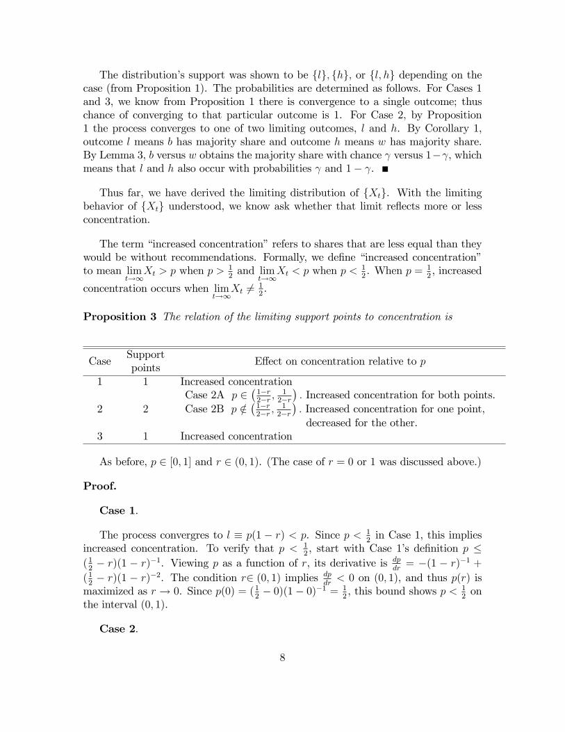
The distribution�s support was shown to be flg; fhg; or fl; hg depending on thecase (from Proposition 1). The probabilities are determined as follows. For Cases 1and 3, we know from Proposition 1 there is convergence to a single outcome; thuschance of converging to that particular outcome is 1. For Case 2, by Proposition1 the process converges to one of two limiting outcomes, l and h. By Corollary 1,outcome l means b has majority share and outcome h means w has majority share.By Lemma 3, b versus w obtains the majority share with chance versus 1� , whichmeans that l and h also occur with probabilities and 1� .
Thus far, we have derived the limiting distribution of fXtg. With the limitingbehavior of fXtg understood, we know ask whether that limit re�ects more or lessconcentration.
The term �increased concentration�refers to shares that are less equal than theywould be without recommendations. Formally, we de�ne �increased concentration�to mean lim
t!1Xt > p when p > 1
2and lim
t!1Xt < p when p < 1
2. When p = 1
2, increased
concentration occurs when limt!1
Xt 6= 12.
Proposition 3 The relation of the limiting support points to concentration is
CaseSupportpoints
E¤ect on concentration relative to p
1 1 Increased concentration
2 2
Case 2A p 2�1�r2�r ;
12�r�: Increased concentration for both points.
Case 2B p =2�1�r2�r ;
12�r�: Increased concentration for one point,decreased for the other.
3 1 Increased concentration
As before, p 2 [0; 1] and r 2 (0; 1). (The case of r = 0 or 1 was discussed above.)
Proof.
Case 1.
The process convergres to l � p(1 � r) < p. Since p < 12in Case 1, this implies
increased concentration. To verify that p < 12, start with Case 1�s de�nition p �
(12� r)(1 � r)�1. Viewing p as a function of r, its derivative is dp
dr= �(1 � r)�1 +
(12� r)(1 � r)�2. The condition r2 (0; 1) implies dp
dr< 0 on (0; 1), and thus p(r) is
maximized as r ! 0. Since p(0) = (12� 0)(1� 0)�1 = 1
2, this bound shows p < 1
2on
the interval (0; 1).
Case 2.
8
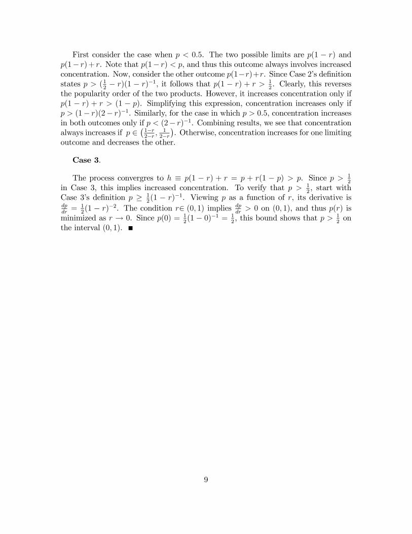
First consider the case when p < 0:5. The two possible limits are p(1 � r) andp(1� r)+ r. Note that p(1� r) < p, and thus this outcome always involves increasedconcentration. Now, consider the other outcome p(1�r)+r. Since Case 2�s de�nitionstates p > (1
2� r)(1 � r)�1, it follows that p(1 � r) + r > 1
2. Clearly, this reverses
the popularity order of the two products. However, it increases concentration only ifp(1 � r) + r > (1 � p). Simplifying this expression, concentration increases only ifp > (1� r)(2� r)�1. Similarly, for the case in which p > 0:5, concentration increasesin both outcomes only if p < (2� r)�1. Combining results, we see that concentrationalways increases if p 2
�1�r2�r ;
12�r�. Otherwise, concentration increases for one limiting
outcome and decreases the other.
Case 3.
The process convergres to h � p(1 � r) + r = p + r(1 � p) > p. Since p > 12
in Case 3, this implies increased concentration. To verify that p > 12, start with
Case 3�s de�nition p � 12(1 � r)�1. Viewing p as a function of r, its derivative is
dpdr= 1
2(1 � r)�2. The condition r2 (0; 1) implies dp
dr> 0 on (0; 1), and thus p(r) is
minimized as r ! 0. Since p(0) = 12(1 � 0)�1 = 1
2, this bound shows that p > 1
2on
the interval (0; 1).
9

Part II: Alternative Simulation Settings
Note on the Simulation
The main simulation and sensitivity were programmed by the authors in Matlab.All code is available on request.
Overview of this Sensitivity Analysis
This section presents sensitivity analyses for the simulation with regard to the mapdistribution, awareness distribution, and the problem size (number of consumers ver-sus products). Sensitivity to the salience parameter �, recommender system employed,and variety seeking were presented in the main paper.
To aid the reader in understanding the parameter space, we have organized theonline appendix by four cases of interest. Any results not covered by these cases areavailable from the authors.
The cases are de�ned by the distributions generating the consumer-product mapsand the awareness states. Within each case, we also vary map parameters, such as thenumber of consumers (I), the number of products (J), and the recommender systemitself.
Review of the Awareness Speci�cation
For reference, we restate the awareness speci�cation used in the paper so thatit can be referred to below. Each consumer is assumed aware of a subset of the Jproducts. Only items in this awareness set can be purchased. The initial awarenessstates for each consumer-product pair are sampled according to
P (ci aware of pj) = �e�distance20j=� + (1� �)e�distance2ij=k�
Above, distance0j and distanceij are respectively the Euclidean distances from theorigin to product pj and from consumer ci to product pj. The constant � 2 [0; 1]. Thehigher is �, the more users are aware of central, mainstream products (left term), andthe higher is 1��, the more users are aware of products in their local neighborhood.The � and �� terms are scaling parameters, determining how fast awareness decayswith distance. Note, this does not mean users are aware of the same products. Theyare likely to overlap in their awareness of the central products but less so in the localones.
Case 1. Normal Consumer-Product Maps. Awareness is central and local.
10

This case is identical to the main paper; we reproduce the results here to facilitatecomparison. The distribution of consumer and product points on the map is standardbivariate normal. The awareness distribution has � = :75, which means consumersare relatively more aware of mainstream goods than niche ones. This assumption isconsistent with a market that has mass advertising, which makes consumers aware of(roughly) the same, central products.
A detailed discussion of the main results was presented in the main paper. Sen-sitivity to the problem size (I; J) did not appear in the main paper and is discussednext. The results are in Table A1 under Case 1.
To start, there are (I; J) = (50; 50) consumers and products.When there are fewerconsumers than products (I = 25; J = 50), G0 is higher than the original (50; 50)case. There are more products for the same number of consumers, and it results thatthere are more products with no or low sales. For example, if consumers always buythe closest product, then more products will have zero sales, yielding a higher Giniin the base case. Although G0 is higher, the change in Gini Gi �G0 is still positive.
When there are more consumers than products (I = 50; J = 25) G0 is lower thanthe original (50,50) case. There are more consumers for the same products, and sofewer products will have zero or low sales. In this case, G0 is lower, but the changein Gini Gi �G0 is still positive as highlighted in Table A1.
When I and J are equal but lower (I = 25; J = 25), G0 is higher than the original(50; 50) case. With fewer data points, by chance some products are closer to moreconsumers; these products have higher sales and so increase the Gini. Conversely,when the map �lls in with many more data points, the chance that some productshave no or low sales decreases and so does the Gini. Again, though the base caseGini di¤ers, the change in Gini Gi �G0 is in the same direction.
Case 2. Normal Consumer-Product Maps. Central Awareness Only.
The distribution of consumer and product points on the map is again standardnormal, as in the main paper. The awareness distribution is identical to the mainpaper except � = 1. This creates a scenario in which users are more aware of centralproducts than peripheral ones. This case provides a robustness check as to whetherdiversity will increase if users are only aware of central products and then discoverthe outer ones via the recommender.
As Table A1-Case 2 shows, concentration in the base case (G0 ) is higher thanin the main paper. This arises because all users are focused on roughly the same,central products. In contrast, in Case 1 users were aware of their local neighborhoodsas well, creating more diversity in the base case. Despite the di¤erences in initialconcentration, the change in Gini is in the same direction: it increases. The above
11

results hold under both r1 and r2. However, the change in Gini is smaller under r2 forthe same reasons as in the main paper. Changing the balance between the numberof consumers (I) and products (J) a¤ects the initial concentration, but it does nota¤ect the sign of Gi �G0, as discussed in Case 1 above.
Case 3. Uniform Consumer-Product Maps. Awareness is central and local.
The distribution of consumer and product points on the map is now uniform ona square centered at the origin and with sides of length four. A box this size (�2in each direction from the origin) roughly captures data from a standard bivariatenormal distribution. This helps change the distribution�s shape without changing itsscale and facilitates comparisons among cases. The awareness distribution is identicalto the main paper: � = :75 again to create the idea that users are aware mainly ofcentral products but also a few local ones.
As Table A1-Case 3 shows, G0 is higher than in the main paper. With theuniform map, products spread out more than in the normal map. Since awarenessstill has a large central component, few people are aware of the now more numerousperipheral products. With more low-selling peripheral products, the initial Gini ishigher. However, despite the higher initial Gini, the change in Gini Gi �G0 is inthe same direction as the main results. Again, the e¤ect under r1 is greater than r2.Imbalances in I versus J have the same e¤ects as described above.
Case 4. Pareto Consumer-Product Maps. Pareto Awareness.
We now test a heavy tailed distribution, the power law. The power law is synony-mous with the Pareto distribution; the former typically refers to the PDF and thelatter to the CDF (Adamic 2000).
The power law distribution has PDF
f(x) = Cx�� =�� 1xmin
�x
xmin
���The restriction x � xmin > 0 is needed for the density to integrate to one. In
addition, � > 2 is required to have a �nite mean.
The consumer and product points are sampled from this density with each point�scoordinate an i.i.d. draw. This distribution creates a roughly L-shaped map. Mostpoints are in the bottom left of the map. There is some spread northward and someeastward, creating an L shape. After generating the maps, they are mean centered.Centering does not a¤ect the shape or inter-point distances; it shifts the origin sothat awareness can be de�ned relative to (0; 0) rather than some other point thatwould change with each map generated. Figure A1 shows an example.
12
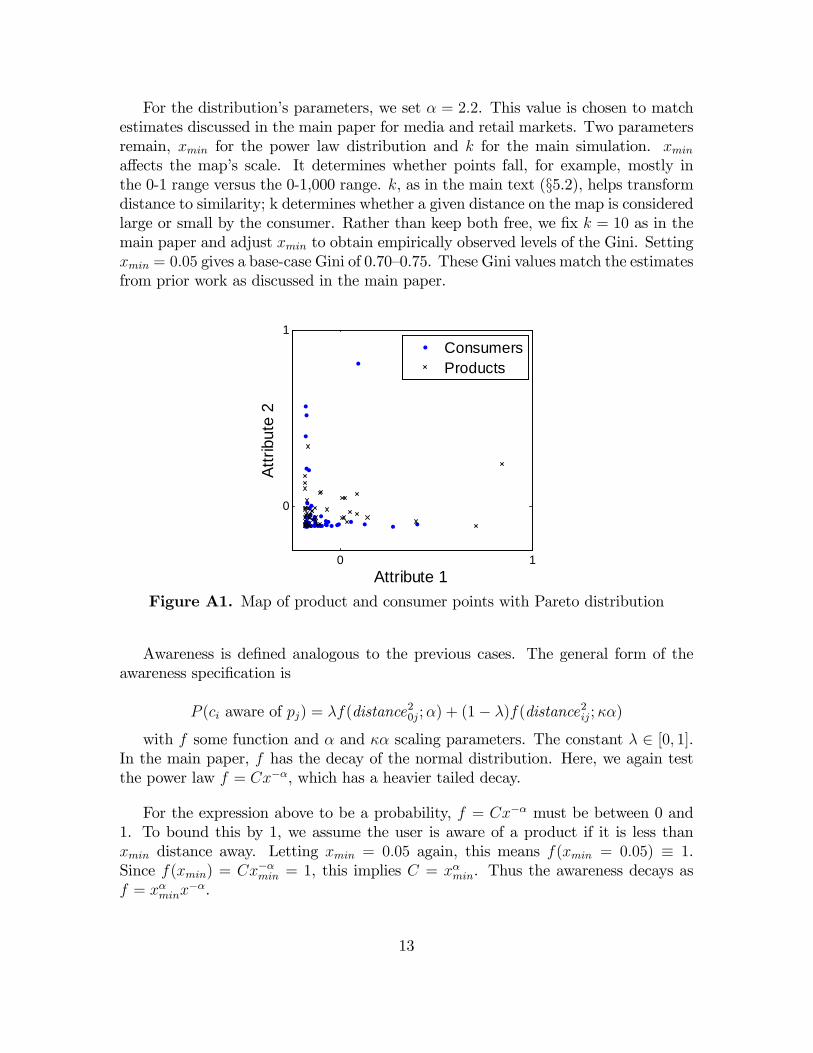
For the distribution�s parameters, we set � = 2:2. This value is chosen to matchestimates discussed in the main paper for media and retail markets. Two parametersremain, xmin for the power law distribution and k for the main simulation. xmina¤ects the map�s scale. It determines whether points fall, for example, mostly inthe 0-1 range versus the 0-1,000 range. k, as in the main text (§5.2), helps transformdistance to similarity; k determines whether a given distance on the map is consideredlarge or small by the consumer. Rather than keep both free, we �x k = 10 as in themain paper and adjust xmin to obtain empirically observed levels of the Gini. Settingxmin = 0:05 gives a base-case Gini of 0.70�0.75. These Gini values match the estimatesfrom prior work as discussed in the main paper.
0 1
0
1
Attribute 1
Attri
bute
2
ConsumersProducts
Figure A1. Map of product and consumer points with Pareto distribution
Awareness is de�ned analogous to the previous cases. The general form of theawareness speci�cation is
P (ci aware of pj) = �f(distance20j;�) + (1� �)f(distance2ij;��)
with f some function and � and �� scaling parameters. The constant � 2 [0; 1].In the main paper, f has the decay of the normal distribution. Here, we again testthe power law f = Cx��, which has a heavier tailed decay.
For the expression above to be a probability, f = Cx�� must be between 0 and1. To bound this by 1, we assume the user is aware of a product if it is less thanxmin distance away. Letting xmin = 0:05 again, this means f(xmin = 0:05) � 1.Since f(xmin) = Cx��min = 1, this implies C = x�min. Thus the awareness decays asf = x�minx
��.
13

For awareness decay relative to the origin, we again use the � = 2:2 estimate. Forawareness decay relative to the consumer�s neighborhood, we use �� = 3�. This isconsistent with the main paper�s goal of making the local awareness neighborhoodsmaller than the center one. (When the local neighborhood is larger than the cen-ter one, consumers know almost every product that might interest them, and therecommender serves no purpose.)
As Table A1-Case 4 shows, despite the di¤erent map, the results are similar. TheGini increases under r1 and r2; imbalances in I versus J have the same e¤ects asdescribed above; and r2 has a smaller e¤ect than r1. However, the e¤ects under bothr1 and r2 are smaller compared with the main paper. In the Pareto maps, there is amass of points in the bottom-left and a few points much farther away. For the largemass, the recommender has the same e¤ects as in Case 1. For the latter, peripheralpoints, they are too spread out for the recommender to be e¤ective. The systemdoes recommend products that a user�s peers purchased, but those products are toofar away for the recommendations to be accepted. As a result, recommendationse¤ectively in�uence only a subset of the population and the change in Gini is less.
In this online appendix, we have tested the sensitivity of our main results underdi¤erent map distributions, di¤erent recommenders, and di¤erent numbers of con-sumers and products. This analysis shows the results to be qualitatively similar tothose discussed in the main paper.
14
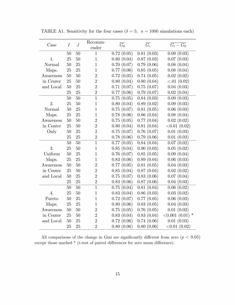
TABLE A1. Sensitivity for the four cases (� = 5; n = 1000 simulations each)
Case I JRecomm-ender
G0 Gi Gi �G050 50 1 0.72 (0.05) 0.81 (0.03) 0.09 (0.03)
1. 25 50 1 0.80 (0.04) 0.87 (0.03) 0.07 (0.03)Normal 50 25 1 0.70 (0.07) 0.79 (0.06) 0.08 (0.04)Maps. 25 25 1 0.77 (0.06) 0.85 (0.05) 0.08 (0.04)
Awareness 50 50 2 0.72 (0.05) 0.74 (0.05) 0.02 (0.02)in Center 25 50 2 0.80 (0.04) 0.80 (0.04) <.01 (0.02)and Local 50 25 2 0.71 (0.07) 0.75 (0.07) 0.04 (0.03)
25 25 2 0.77 (0.06) 0.79 (0.07) 0.02 (0.04)50 50 1 0.75 (0.05) 0.84 (0.03) 0.09 (0.03)
2. 25 50 1 0.80 (0.04) 0.89 (0.02) 0.09 (0.03)Normal 50 25 1 0.75 (0.07) 0.81 (0.05) 0.06 (0.03)Maps. 25 25 1 0.78 (0.06) 0.86 (0.04) 0.08 (0.04)
Awareness 50 50 2 0.75 (0.05) 0.77 (0.04) 0.02 (0.02)in Center 25 50 2 0.80 (0.04) 0.81 (0.04) <0.01 (0.02)Only 50 25 2 0.75 (0.07) 0.76 (0.07) 0.01 (0.03)
25 25 2 0.78 (0.06) 0.79 (0.06) 0.01 (0.03)50 50 1 0.77 (0.05) 0.84 (0.04) 0.07 (0.02)
3. 25 50 1 0.85 (0.04) 0.90 (0.03) 0.05 (0.02)Uniform 50 25 1 0.76 (0.07) 0.85 (0.05) 0.09 (0.04)Maps. 25 25 1 0.83 (0.06) 0.89 (0.04) 0.06 (0.03)
Awareness 50 50 2 0.77 (0.05) 0.81 (0.05) 0.04 (0.03)in Center 25 50 2 0.85 (0.04) 0.87 (0.04) 0.02 (0.02)and Local 50 25 2 0.75 (0.07) 0.83 (0.06) 0.07 (0.04)
25 25 2 0.83 (0.06) 0.87 (0.06) 0.04 (0.03)50 50 1 0.75 (0.04) 0.81 (0.04) 0.06 (0.02)
4. 25 50 1 0.83 (0.04) 0.86 (0.03) 0.03 (0.02)Pareto 50 25 1 0.72 (0.07) 0.77 (0.05) 0.06 (0.03)Maps. 25 25 1 0.80 (0.06) 0.83 (0.05) 0.04 (0.03)
Awareness 50 50 2 0.75 (0.05) 0.76 (0.05) 0.01 (0.02)in Center 25 50 2 0.83 (0.04) 0.83 (0.04) <0.001 (0.01) *and Local 50 25 2 0.72 (0.06) 0.74 (0.06) 0.01 (0.03)
25 25 2 0.80 (0.06) 0.80 (0.06) <0.01 (0.02)
All comparisons of the change in Gini are signi�cantly di¤erent from zero (p < 0:05)except those marked * (t-test of paired di¤erences for zero mean di¤erence).
15
References
[1] Adamic, L. A. 2000. Zipf, Power-law, Pareto: a ranking tutorial. HP Research.http://www.hpl.hp.com/research/idl/papers/ranking/. Accessed April 6, 2008.
[2] Durrett, R. 2005. Probability: Theory and Examples. Belmont, CA: ThompsonBrooks�Cole.
[3] Hill, B. M., D. Lane, and W. Sudderth. 1980. A strong law for some generalizedurn processes. Annals of Probability 8(2):214-226
16


