Bridge Pier Flow Interaction and Its Effect
on the Process of Scouring
By
Chij Kumar Shrestha
A thesis submitted in fulfilment
of the requirement for the degree of
Doctor of Philosophy
Faculty of Engineering and Information Technology
University of Technology Sydney (UTS)
September 2015

Bridge Pier – Flow Interaction and Its Effect on the Process of Scouring i
CERTIFICATE OF ORIGINAL AUTHORSHIP
I certify that the work in this thesis has not previously been submitted for a degree nor
has it been submitted as part of requirements for a degree except as fully
acknowledged within the text.
I also certify that the thesis has been written by me. Any help that I have received in
my research work and the preparation of the thesis itself has been acknowledged. In
addition, I certify that all information sources and literature used are indicated in the
thesis.
Chij Kumar Shrestha
Sydney, September 2015

Bridge Pier – Flow Interaction and Its Effect on the Process of Scouring ii
ABSTRACT
Previous investigations indicate that scour around bridge piers is a contributor in the
failure of waterway bridges. Hence, it is essential to determine the accurate scour depth
around the bridge piers. For this purpose, deep understanding of flow structures around
bridge piers is very important. A number of studies on flow structures and local scour
around bridge piers have been conducted in the past. Most of the studies, carried out to
develop a design criterion, were based on a single column. However, in practice, bridge
piers can comprise multiple columns that together support the bridge superstructure.
Typically, the columns are aligned in the flow direction. The design criteria developed
for a single column ignore the most important group effects for multiple columns cases
such as sheltering, reinforcement and interference effects. These group effects can
significantly be influenced by the variation of spacing between two columns. This is
evident by the fact that insufficient investigations and development have been reported
for the flow structure and maximum scour depth around bridge piers comprising multiple
columns. It is therefore necessary to investigate the effects of multiple columns and
spacing between them on the flow structure and local scour around bridge piers and
develop a practical method to predict the maximum scour depth.
The main objectives of this research work are to analyse the effect of spacing between
two in-line circular columns on the flow structure and to develop a reliable method for
prediction of the maximum local scour depth around bridge piers. To meet the objectives
this research, detailed experimental studies on three dimensional flow structures and local
scour around two-column bridge piers were carried out. A series of laboratory
experiments were conducted for no column, a single column and two in-line columns
cases with different spacing. Two in-line columns were installed at the centre of the flume
along the longitudinal axis. Three dimensional flow velocities in three different horizontal
planes were measured at different grid points within the flow using a micro acoustic
doppler velocimeter (ADV). The velocity was captured at a frequency of 50Hz.
Additionally, in vertical planes, particle image velocimetry (PIV) technique was
employed to measure the two dimensional instantaneous velocity components. All
experiments on flow structures were conducted under no scouring and clear water flow
Bridge Pier – Flow Interaction and Its Effect on the Process of Scouring iii
conditions. Similarly, an array of experimental tests were conducted under different flow
conditions for studying the temporal development of scour depth and the maximum local
scour depth around a single column and two-column bridge piers.
The measured instantaneous three dimensional velocity components were analysed and
the results for flow field and turbulence characteristics were presented in graphical forms
using vector plots, streamline plots, contour plots and profile plots. The results indicated
that the flow structures around two- columns bridge piers is more complex than that of a
single column case. Furthermore, the spacing between two columns significantly affects
the flow structures, particularly in the wake of the columns. It was observed that for the
spacing-column diameter ratio (L/D) < 3, the vortex shedding occurred only behind the
downstream column. Hence, the flow pattern was more or less similar to that of the single
column case. However, the turbulence characteristics such as turbulence intensity,
turbulent kinetic energy and Reynolds shear stresses were notably different from those of
a single column case. When the spacing was in the range of 2 ≤ L/D ≤ 3, stronger
turbulence structures were noticed behind the upstream column. Further increase in the
spacing between two columns resulted in a decrease in the strength of turbulence
characteristics.
The experimental results on temporal development of local scour depth reveal that
approximately 90% of the maximum scour depth around the upstream column was
achieved within the first 10 hours of the experiments. However, for the downstream
column, 90% of the scour depth was achieved within 20 hours. Similarly, the results from
the experiments on local scour indicated that the maximum scour depth occurred at the
upstream column, when the spacing between two columns was 2.5D. The maximum value
of local scour depth for the two-column case was observed about 18% higher than the
value obtained for the single column case. The reasons for maximum scour depth at the
spacing of 2.5D were identified as the reinforcing effect of downstream column, the
strong horseshoe vortex at upstream column, strong turbulence characteristics at the wake
of upstream column, and the highest probability of occurrence of sweep events at
upstream side of upstream column. Furthermore, a semi empirical equation was
developed to predict the maximum scour depth as a function of the spacing between two

Bridge Pier – Flow Interaction and Its Effect on the Process of Scouring iv
columns. The findings of this study can be used to facilitate the position of columns when
scouring is a design concern.

Bridge Pier – Flow Interaction and Its Effect on the Process of Scouring v
ACKNOWLEDGMENT
This thesis could not be completed without the assistance, understanding and counselling
of several people throughout the research work. I would like to express my sincere
gratitude to my supervisors, Associate Professor Hadi Khabbaz and Professor Alireza
Keshavarzi for their support and guidance during my PhD study. Apart from the academic
supervision, inspiring suggestions for work-family life balance and future career
development from my supervisors were the important factors for successful completion
of my thesis.
I would like to express my sincere thanks to Dr. Behzad Fatahi for coordinating my
Doctoral Assessment and for his valuable suggestions. I cannot forget external and
internal assessors Dr. Farzad Meysami and Dr. Hamid Valipour, respectively for
evaluating my Doctoral Assessment report and providing constructive recommendations.
My sincere thanks also go to Professor Bruce W. Melville and Associate Professor James
Ball for their great contributions and suggestions as co-authors for the publication of
conference and Journal papers. Furthermore, I would like to thank Mr. Rami Haddad and
Mr. David Hooper for their valuable support for smooth conduction of the experimental
tests in the Hydraulics Laboratory. I would also like to thank my close friends Dr. Aslan
Hokmabadi and Dr. Md. Mahbube Subhani for sharing their time and friendship to make
a life more fun and easy.
I am greatly indebted to my parents, my brother Manoj and my sister Shanti for their love,
support and encouragement. Without their many years of encouragement and support, I
may never have reached where I am today. They always refuel me with courage and
inspiration to overcome any hardship encountered in my life. Most importantly, I am
extremely indebted to my wife Chandra Laxmi Shrestha for her great love, kind patience
and invaluable support. Thank you very much for your sacrifice in shouldering far more
than your fair share of parenting and for being a vital source of encouragement when I
feel lack of faith and energy.
Finally, I would be remiss if I did not acknowledge my son Charchit and daughter Chaarvi
for their understanding, love and affection throughout my PhD research.

Bridge Pier – Flow Interaction and Its Effect on the Process of Scouring vi
LIST OF PUBLICATIONS BASED ON THIS RESEARCH
Peer-reviewed Conference Papers
1. SHRESTHA, C. K., KESHAVARZI, A., KHABBAZ, H. & BALL, J. 2012.
Experimental Study of the Flow Structure Interactions between Bridge Piers 34th
Hydrology and Water Resources Symposium (HWRS 2012), Sydney, Australia.
2. SHRESTHA, C. K., KESHAVARZI, A. & KHABBAZ, H. 2013. Flow Structure at
Downstream Side of Two Sequential Bridge Piers. In: Shoji Fukuoka, Hajime
Nakagawa, Tetsuya Sumi & Hao Zhang, eds. International Symposium on River
Sedimentation (ISRS 2013), Kyoto, Japan. CRC Press/Balkema, 199.
3. SHRESTHA, C. K., KESHAVARZI, A. & KHABBAZ, H. 2013. Experimental
Study of Bridge -Pier Interaction and its Effect on Bed Scour 6th International
Perspective on Water Resources and the Environment (IPWE 2013), Izmir, Turkey.

Bridge Pier – Flow Interaction and Its Effect on the Process of Scouring vii
CONTENTS
CERTIFICATE OF ORIGINAL AUTHORSHIP ........................................................ i
ABSTRACT ..................................................................................................................... ii
ACKNOWLEDGMENT ................................................................................................ v
LIST OF PUBLICATIONS BASED ON THIS RESEARCH ................................... vi
CONTENTS ................................................................................................................... vii
LIST OF NOTATIONS ............................................................................................. xxiii
1. INTRODUCTION ....................................................................................................... 2
1.1 Background ................................................................................................................. 2
1.2 Research Objectives .................................................................................................... 5
1.3 Scope and Limitation of Research .............................................................................. 6
1.4 Research Significance and Innovation ........................................................................ 6
1.5 Research Methodology................................................................................................ 7
1.6 Synopsis of Thesis ...................................................................................................... 8
2. LITERATURE REVIEW ......................................................................................... 11
2.1 Introduction ............................................................................................................... 11
2.2 Scour at Bridge Crossings ......................................................................................... 11
2.2.1 General Scour ................................................................................................... 12
2.2.2 Localised Scour ................................................................................................ 13
2.3 Sediment Transport and Local Scour around Bridge Piers ....................................... 13
2.3.1 Basics of Sediment Transport ........................................................................... 13
2.3.2 Local Scour around Bridge Piers ..................................................................... 24
Bridge Pier – Flow Interaction and Its Effect on the Process of Scouring viii
2.3.3 Mechanism of Local Scour ............................................................................... 26
2.3.4 Parameters for Analysis of Pier Scour ............................................................. 29
2.3.5 Factors Affecting the Local Scour at Bridge Site ............................................. 31
2.3.6 Equilibrium Scour Depth .................................................................................. 43
2.3.7 Temporal Variation of Scour Depth ................................................................. 44
2.3.8 Estimation of Equilibrium Scour Depth ........................................................... 47
2.4 Open Channel Flow and Flow around Bridge Piers ................................................. 58
2.4.1 Hydraulics of Open Channel Flow ................................................................... 58
2.4.2 Basic Equations for Flow in Open Channels ................................................... 60
2.4.3 Boundary Layer in Open Channel Flow .......................................................... 63
2.4.4 Turbulence in Open Channel Flow .................................................................. 65
2.4.5 Flow around Bridge Piers ................................................................................ 66
2.5 Summary and Identification of the Gap in Literature ............................................... 78
3. EXPERIMENTAL SETUP AND METHODOLOGY .......................................... 82
3.1 Introduction ............................................................................................................... 82
3.2 Experimental Setup and Design ................................................................................ 82
3.2.1 Flume and its Components ............................................................................... 82
3.2.2 Electromagnetic Flow Meter ............................................................................ 84
3.2.3 Vernier Point Gauge......................................................................................... 84
3.2.4 Model Columns of Bridge Piers ....................................................................... 85
3.2.5 Bed Materials ................................................................................................... 86

Bridge Pier – Flow Interaction and Its Effect on the Process of Scouring ix
3.2.6 Flow Conditions ............................................................................................... 87
3.3 Velocity Measurement .............................................................................................. 89
3.3.1 Acoustic Doppler Velocimetry (ADV) .............................................................. 89
3.3.2 Particle Image Velocimetry (PIV) .................................................................... 91
3.4 Experimental Procedure and Data Acquisition ......................................................... 94
3.4.1 Procedure for Fixed Bed Experiments in Flume 1 ........................................... 94
3.4.2 Procedure for Mobile Bed Experiments in Flume 1 ......................................... 97
3.4.3 Procedure for Fixed Bed Experiments in Flume 2 ........................................... 97
3.5 Summary ................................................................................................................... 99
4. RESULTS AND DISCUSSION ON FLOW STRUCTURE ............................... 102
4.1 Introduction ............................................................................................................. 102
4.2 Previous Investigations on Flow around Bridge Piers ............................................ 102
4.3 Flow around the Bridge Piers in Horizontal Plane.................................................. 106
4.3.1 Flow Pattern ................................................................................................... 107
4.3.2 Three Dimensional Velocity Component ........................................................ 110
4.3.3 Turbulence Intensity ....................................................................................... 124
4.3.4 Turbulent Kinetic Energy ............................................................................... 132
4.3.5 Reynolds Shear Stresses ................................................................................. 135
4.4 Flow around the Bridge Piers in Vertical Plane ...................................................... 138
4.4.1 Flow Pattern ................................................................................................... 140
4.4.2 Time Average Velocity Components ............................................................... 145

Bridge Pier – Flow Interaction and Its Effect on the Process of Scouring x
4.4.3 Turbulence Intensity Components .................................................................. 156
4.4.4 Turbulent Kinetic Energy ............................................................................... 166
4.4.5 Reynolds Shear Stresses ................................................................................. 171
4.5 Bursting Phenomenon and Quadrant Analysis ....................................................... 175
4.5.1 Introduction .................................................................................................... 175
4.5.2 Review on Quadrant Analysis ........................................................................ 176
4.5.3 Results of Quadrant Analysis ......................................................................... 181
4.6 Summary ................................................................................................................. 191
5. RESULTS AND DISCUSSION ON LOCAL SCOUR ........................................ 196
5.1 Introduction ............................................................................................................. 196
5.2 Previous Investigations on Scour around Bridge Piers ........................................... 196
5.3 Temporal Development of Scour Depth ................................................................. 199
5.4 Equilibrium Scour Depth for Two-Column Case ................................................... 202
5.5 Comparison of Observed and Predicted Maximum Scour Depths ......................... 209
5.6 Scour Profile along Centerline of the Bridge Piers ................................................. 211
5.7 Width of the Scour Hole ......................................................................................... 213
5.8 Summary ................................................................................................................. 215
6. CONCLUSION AND RECOMMENDATIONS .................................................. 219
6.1 Introduction ............................................................................................................. 219
6.2 Conclusions ............................................................................................................. 219
6.3 Recommendations of Future Research ................................................................... 225
REFERENCES ............................................................................................................ 227
APPENDIX-A: PLOTS FOR VELOCITY COMPONENTS ................................. 243

Bridge Pier – Flow Interaction and Its Effect on the Process of Scouring xi
A.1 Plots of Velocity Components in Horizontal Plane ............................................... 243
A.2 Plots of Velocity Components for Vertical Plane. ................................................. 274
A.3 Table of Results on Velocity Components ............................................................. 297
APPENDIX-B: PLOTS FOR TURBULENCE INTENSITIES .............................. 303
B.1 Plots of Turbulence Intensity in Horizontal Plane ................................................. 303
B.2 Plots of Turbulence Intensity in Vertical Plane ...................................................... 324
B.3 Table of Results on Turbulence Intensity Components ......................................... 340
APPENDIX-C: PLOTS FOR TURBULENT KINETIC ENERGY ....................... 346
C.1 Plots of Turbulent Kinetic Energy in Horizontal Plane.......................................... 346
C.2 Plots of Turbulent Kinetic Energy in Vertical Plane .............................................. 355
C.3 Table of Results on Turbulent Kinetic Energy ....................................................... 363
APPENDIX-D: PLOTS FOR REYNOLDS STRESSES ......................................... 364
D.1 Profile Plots of Reynolds Stresses in Horizontal Plane.......................................... 364
D.2 Plots of Reynolds Stresses in Vertical Plane .......................................................... 368
D.3 Table of Results on Reynolds Shear Stresses ........................................................ 376
APPENDIX-E PLOTS FOR QUADRANT ANALYSIS ......................................... 378
E.1 Probability of Occurrence of the Events at Upstream and Downstream sides ....... 378
E.2 Profile Plots for Stress Fraction Contribution of the Events for the Production of
Reynolds Stress. ................................................................................................... 388

Bridge Pier – Flow Interaction and Its Effect on the Process of Scouring xii
LIST OF FIGURES
Figure 1.1 Bridge piers experiencing the flood events (USGS (2014) ............................. 4
Figure 1.2 a) Scour around bridge piers on the Logan river, Australia; (Queensland
Government (2013) ; and b) Scour around bridge piers on the Tinau river, Nepal, (KC
(2014) ................................................................................................................................ 4
Figure 1.3 A bridge over the Gaula river in India washed away by flood in July 2008,
(Bhatia (2013) ................................................................................................................... 5
Figure 2.1 Types of scour at a bridge, (after Melville and Coleman, 2000) ................... 11
Figure 2.2 Classification of scour (after Melville and Coleman, 2000).......................... 12
Figure 2.3 Local scour at bridge piers; (Vasquz, 2006) .................................................. 13
Figure 2.4 Threshold condition for the sediment entrainment ........................................ 15
Figure 2.5 Shields diagram for incipient motion of sediment (after Simons and Senturk,
1992) ............................................................................................................................... 17
Figure 2.6 Shear velocity chart for quartz sediment in water at 20° C; (after Melville
and Coleman, 2000) ........................................................................................................ 18
Figure 2.7 Definition sketch of suspended load transport; (after Van Rijn, 1993) ......... 22
Figure 2.8 Shape factor for different suspension numbers; (after Van Rijn, 1993) ........ 23
Figure 2.9 Local scour around bridge piers as a function of time; (after Richardson and
Davis, 2001) .................................................................................................................... 25
Figure 2.10 Flow field around bridge piers, (Ettema et al., 2011) .................................. 27
Figure 2.11 Influence of flow shallowness on local scour depth, (after Melville and
Coleman, 2000) ............................................................................................................... 33
Figure 2.12 Effect of sediment coarseness on local scour; (after Melville and Coleman,
2000) ............................................................................................................................... 34
Figure 2.13 Effect of sediment non-uniformity on local scour at bridge piers under clear
water condition; (after Melville and Coleman, 2000) ..................................................... 35

Bridge Pier – Flow Interaction and Its Effect on the Process of Scouring xiii
Figure 2.14 Variation of local scour depth with sediment non-uniformity, (after Melville
and Coleman, 2000) ........................................................................................................ 36
Figure 2.15 Basic pier shapes; (after Ettema et al., 2011) .............................................. 37
Figure 2.16 Variation of local scour depth with pier alignment; (after Melville and
Coleman, 2000) ............................................................................................................... 38
Figure 2.17 Variation of local scour depth with flow intensity, V/Vc , (after Melville and
Coleman, 2000) ............................................................................................................... 39
Figure 2.18 Effect of flow intensity on local scour depth in uniform sediment (after
Melville and Coleman, 2000) .......................................................................................... 40
Figure 2.19 Effect of flow intensity on local scour depth in non-uniform sediment (after
Melville and Coleman, 2000) .......................................................................................... 41
Figure 2.20 Variation of scour depth with Froude number; (after Ettema et al., 2006) . 42
Figure 2.21 Time development of scour depth under clear water and live bed conditions;
(after Ettema et al., 2011) ................................................................................................ 43
Figure 2.22 Temporal development of scour depth; (after Melville and Chiew, 1999) . 46
Figure 2.23 Notations for continuity equations; (after Chaudhry, 2007) ........................ 61
Figure 2.24 Notations for momentum equations and application; (after Chaudhry, 2007)
......................................................................................................................................... 61
Figure 2.25 Notations for energy equations .................................................................... 63
Figure 2.26 Development of boundary layer in open channel (Simons, 1992) .............. 64
Figure 2.27 Definition sketch of flow regions; (after Sumer and Fredsoe, 1997) .......... 69
Figure 2.28 Flow regimes around smooth circular cylinder in steady current, (Sumer
and Fredsoe, 1997) .......................................................................................................... 72
Figure 2. 29 Definition sketch of flow interference region for two cylinders
arrangements; (after Sumner, 2010) ................................................................................ 73
Figure 2.30 Classification of flow regimes for two tandem cylinders; (after Sumner,
2010) ............................................................................................................................... 73

Bridge Pier – Flow Interaction and Its Effect on the Process of Scouring xiv
Figure 2.31 Schematics of vortex shedding a) Prior to shedding of Vortex A, Vortex B
is being drawn across the wake, b) Prior to shedding of Vortex B, Vortex C is being
drawn across the wake (Sumer and Fredsoe, 1997) ........................................................ 77
Figure 2.32 Strouhal number as a function of Reynolds number; (Sumer and Fredsoe,
1997) ............................................................................................................................... 78
Figure 3.1 Schematic diagram of Flume 1 ...................................................................... 83
Figure 3.2 Schematic diagram of Flume 2 ...................................................................... 83
Figure 3.3 Electromagnetic flow meter (courtesy of Siemens)....................................... 84
Figure 3.4 Vernier point gauge to measure the scour depth ........................................... 85
Figure 3.5 Model columns showing the spacing between them ..................................... 85
Figure 3.6 Grain size distribution curve of the sand used ............................................... 87
Figure 3.7 Velocity measurement a) Acoustic Doppler Velocimeter (ADV) ( SonTek
(2012), and b) measuring velocity in laboratory ............................................................. 90
Figure 3.8 ADV probe and signal processor in splash proof housing (SonTek (2012) .. 91
Figure 3.9 Schematic illustration of PIV system, (ILA-GmbH (2004)........................... 92
Figure 3.10 Digital charged coupled device (CCD) camera,(PCO-TECH (2008) ......... 93
Figure 3.11 Laser source and the controlling system: a) laser head with mirrored arm
(ILA-GmbH), and b) ICE450 power supply system (Quantel (2006) ............................ 94
Figure 3.12 Measurement grid in horizontal plane (top view) ....................................... 96
Figure 3.13 Different axes of PIV measurements (top view) ......................................... 98
Figure 4.1 Definition sketch of the bridge piers arrangement ...................................... 106
Figure 4.2 Schematic diagram of different axis of data analysis in horizontal planes .. 107
Figure 4.3 Flow pattern around a single column in horizontal plane at Z/h = 0.09 a)
Vector plot, and b) Streamline plot ............................................................................... 108
Bridge Pier – Flow Interaction and Its Effect on the Process of Scouring xv
Figure 4.4 Flow pattern around two columns with L/D = 3 in horizontal plane at Z/h =
0.09 a) Vector plot, and b) Streamline plot .................................................................. 109
Figure 4.5 Contour plots of streamwise velocity component for the single column case
in different horizontal planes a) at Z/h = 0.09, b) at Z/h = 0.26 and c). at Z/h = 0.54 .. 111
Figure 4.6 Profile plots of streamwise velocity component for the single column case in
different horizontal planes along three different longitudinal axes a) at Z/h = 0.09, b) at
Z/h = 0.26 and c). at Z/h = 0.54 .................................................................................... 112
Figure 4.7 Contour plots of streamwise velocity component for two columns case with
L/D = 3 in different horizontal planes a) at Z/h = 0.09, b) at Z/h = 0.26 and c). at Z/h =
0.54 ................................................................................................................................ 113
Figure 4.8 Profile plots of the streamwise velocity component for two-column case with
L/D = 3 in different horizontal planes along three different longitudinal axes a) at Z/h =
0.09, b) at Z/h = 0.26 and c). at Z/h = 0.54 ................................................................... 114
Figure 4.9 Contour plots of transverse velocity component for the single column case in
different horizontal planes a) at Z/h = 0.09, b) at Z/h = 0.26 and c). at Z/h = 0.54 ...... 115
Figure 4.10 Profile plots of transverse velocity component for the single column case in
different horizontal planes along three different longitudinal axes a) at Z/h = 0.09, b) at
Z/h = 0.26 and c). at Z/h = 0.54 .................................................................................... 116
Figure 4.11 Contour plots of transverse velocity component for the two-column case
with L/D = 3 in different horizontal planes a) at Z/h = 0.09, b) at Z/h = 0.26 and c). at
Z/h = 0.54 ...................................................................................................................... 117
Figure 4.12 Profile plots of transverse velocity component for the two-column case with
L/D = 3 in different horizontal planes along three different longitudinal axes a) at Z/h =
0.09, b) at Z/h = 0.26 and c). at Z/h = 0.54 ................................................................... 118
Figure 4.13 Contour plots of vertical velocity component for the single column case in
different horizontal planes a) at Z/h = 0.09, b) at Z/h = 0.26 and c). at Z/h = 0.54 ...... 120
Figure 4.14 Profile plots of vertical velocity component for the single column case in
different horizontal planes along three different longitudinal axes a) at Z/h = 0.09, b) at
Z/h = 0.26 and c). at Z/h = 0.54 .................................................................................... 121

Bridge Pier – Flow Interaction and Its Effect on the Process of Scouring xvi
Figure 4.15 Contour plots of vertical velocity component for the two-column case with
L/D = 3 in different horizontal planes a) at Z/h = 0.09, b) at Z/h = 0.26 and c). at Z/h =
0.54 ................................................................................................................................ 122
Figure 4.16 Profile plots of vertical velocity component for the two-column case with
L/D = 3 in different horizontal planes along three different longitudinal axes a) at Z/h =
0.09, b) at Z/h = 0.26 and c). at Z/h = 0.54 ................................................................... 123
Figure 4.17 Contour plots of streamwise turbulence component for the single column
case in different horizontal planes a) at Z/h = 0.09, b) at Z/h = 0.26 and c). at Z/h = 0.54
....................................................................................................................................... 124
Figure 4.18 Profile plots of streamwise turbulence intensity component for the single
column case in different horizontal planes along three different longitudinal axes a) at
Z/h = 0.09, b) at Z/h = 0.26 and c). at Z/h = 0.54 ......................................................... 125
Figure 4.19 Contour plots of streamwise turbulence intensity component for the two-
column case with L/D = 3 in different horizontal planes a) at Z/h = 0.09, b) at Z/h =
0.26 and c). at Z/h = 0.54 .............................................................................................. 126
Figure 4.20 Profile plots of streamwise turbulence intensity component for the two-
column case with L/D = 3 in different horizontal planes along three different
longitudinal axes a) at Z/h = 0.09, b) at Z/h = 0.26 and c). at Z/h = 0.54 ..................... 127
Figure 4.21 Contour plots of transverse turbulence intensity component for the single
column case in different horizontal planes a) at Z/h = 0.09, b) at Z/h = 0.26 and c). at
Z/h = 0.54 ...................................................................................................................... 128
Figure 4.22 Contour plots of transverse turbulence intensity component for the two-
column case with L/D = 3 in different horizontal planes a) at Z/h = 0.09, b) at Z/h =
0.26 and c). at Z/h = 0.54 .............................................................................................. 129
Figure 4.23 Contour plots of vertical turbulence intensity component for the single
column case in different horizontal planes a) at Z/h = 0.09, b) at Z/h = 0.26 and c). at
Z/h = 0.54 ...................................................................................................................... 130
Bridge Pier – Flow Interaction and Its Effect on the Process of Scouring xvii
Figure 4.24 Contour plots of vertical turbulence intensity component for the two-
column case with L/D = 3 in different horizontal planes a) at Z/h = 0.09, b) at Z/h =
0.26 and c). at Z/h = 0.54 .............................................................................................. 131
Figure 4.25 Contour plots of turbulent kinetic energy for the single column case in
different horizontal planes a) at Z/h = 0.09, b) at Z/h = 0.26 and c). at Z/h = 0.54 ...... 134
Figure 4.26 Contour plots of turbulent kinetic energy for the two-column case with L/D
= 3 in different horizontal planes a) at Z/h = 0.09, b) at Z/h = 0.26 and c). at Z/h = 0.54
....................................................................................................................................... 135
Figure 4.27 Profile plots of Reynold shear stresses for the single column case in
different horizontal planes along axis of symmetry a) in u-v plane, b) in u-w plane, and
c) in v-w plane ............................................................................................................... 136
Figure 4.28 Profile plots of Reynolds shear stresses for two-column case with L/D = 3
in different horizontal planes along axix of symmetry a) in u-v plane, b) in u-w plane,
and c) in v-w plane ........................................................................................................ 137
Figure 4.29 Schematic diagram of different axis of data analysis at upstream and
downstream side of the columns in vertical planes (US, B and DS stand for upstream
side, between and downstream side of the columns, respectively) ............................... 139
Figure 4.30 Vector plots for single column a) vertical plane at Y/D = 0, and b) vertical
plane at Y/D = 1.25 ....................................................................................................... 142
Figure 4.31 Vector plots for two columns cases with L/D = 3 a) vertical plane at Y/D =
0, and b) vertical plane at Y/D = 1.25 ........................................................................... 143
Figure 4.32 Streamline plots for single column a) vertical plane at Y/D = 0, and b)
vertical plane at Y/D = 1.25 .......................................................................................... 144
Figure 4.33 Streamline plots for two columns cases with L/D = 3 a) vertical plane at
Y/D = 0, and b) vertical plane at Y/D = 1.25 ................................................................ 145
Figure 4.34 Contour plots of streamwise velocity component for the single column case
in different vertical planes a) at Y/D = 0, and b) at Y/D = 1.25 ................................... 146
Figure 4.35 Profile plots of streamwise velocity component for the single column case
in vertical plane at axis of symmetry a) upstream side; b) downstream side ................ 147

Bridge Pier – Flow Interaction and Its Effect on the Process of Scouring xviii
Figure 4.36 Contour plots of streamwise velocity component for the case of two in-line
columns with L/D = 3 in different vertical planes a) at Y/D = 0, and b) at Y/D = 1.25
....................................................................................................................................... 149
Figure 4.37 Profile plots of streamwise velocity component for two columns case with
L/D = 3 in vertical plane at axis of symmetry a) upstream side; b) downstream side .. 150
Figure 4.38 Profile plots of velocity components between two columns with L/D = 3 in
vertical plane at axis of symmetry a) streamwise component, b) vertical component . 150
Figure 4.39 Contour plots of vertical velocity component for single column case in
different vertical planes a) at Y/D = 0, and b) at Y/D = 1.25 ....................................... 152
Figure 4.40 Profile plots of vertical velocity component for single column case in
vertical plane at axis of symmetry a) upstream side; b) downstream side .................... 153
Figure 4.41 Contour plots of vertical velocity component for the two-column case with
L/D = 3 in different vertical planes a) at Y/D = 0, and b) at Y/D = 1.25 ...................... 154
Figure 4.42 Profile plots of vertical velocity component for the two-column case with
L/D = 3 in vertical plane at axis of symmetry a) upstream side; b) downstream side .. 155
Figure 4.43 Profile plots of velocity components between two columns with L/D = 3 in
vertical plane at axis of symmetry a) streamwise component, b) vertical component . 156
Figure 4.44 Contour plots of streamwise turbulence intensity component for the single
column case in different vertical planes a) at Y/D = 0, and b) at Y/D = 1.25 .............. 157
Figure 4.45 Profile plots of streamwise turbulence intensity component for the single
column case in vertical plane at axis of symmetry a) upstream side; b) downstream side
....................................................................................................................................... 158
Figure 4.46 Contour plots of streamwise turbulence intensity component for two
columns case with L/D = 3 in different vertical planes a) at Y/D = 0, and b) at Y/D =
1.25 ................................................................................................................................ 159
Figure 4.47 Profile plots of streamwise turbulence intensitycomponent for two-column
case with L/D = 3 in vertical plane at axis of symmetry a) upstream side, b) downstream
side, and c) between two columns................................................................................. 161
Bridge Pier – Flow Interaction and Its Effect on the Process of Scouring xix
Figure 4.48 Contour plots of vertical turbulence intensity component for the single
column case in different vertical planes a) at Y/D = 0, and b) at Y/D = 1.25 .............. 162
Figure 4.49 Profile plots of vertical turbulence intensity component for the single
column case in vertical plane at axis of symmetry a) upstream side; b) downstream side
....................................................................................................................................... 163
Figure 4.50 Contour plots of vertical turbulence intensity component for two columns
case with L/D = 3 in different vertical planes a) at Y/D = 0, and b) at Y/D = 1.25 ...... 164
Figure 4.51 Profile plots of vertical turbulence intensity component for the case of two
in-line columns with L/D = 3 in vertical plane at axis of symmetry a) upstream side, b)
downstream side, and c) between two columns ............................................................ 165
Figure 4.52 Contour plots of turbulent kinetic energy for the single column case in
different vertical planes a) at Y/D = 0, and b) at Y/D = 1.25 ....................................... 167
Figure 4.53 Profile plots of turbulent kinetic energy for the single column case in
vertical plane at axis of symmetry a) upstream side; b) downstream side .................... 168
Figure 4.54 Contour plots of turbulent kinetic energy for the two-column case with L/D
= 3 in different vertical planes a) at Y/D = 0, and b) at Y/D = 1.25 ............................. 169
Figure 4.55 Profile plots of turbulent kinetic energy for the case of two in-line columns
with L/D = 3 in vertical plane at axis of symmetry a) upstream side, b) downstream
side, and c) between two columns................................................................................. 170
Figure 4.56 Contour plots of Reynolds shear stress for the single column case in
different vertical planes a) at Y/D = 0, and b) at Y/D = 1.25 ....................................... 171
Figure 4.57 Profile plots of Reynolds shear stress for the single column case in vertical
plane at axis of symmetry a) upstream side; b) downstream side ................................. 172
Figure 4.58 Contour plots of Reynolds shear stress for the case of two in-line columns
with L/D = 3 in different vertical planes a) at Y/D = 0, and b) at Y/D = 1.25 .............. 173
Figure 4.59 Profile plots of Reynolds shear stress for the two-column case with L/D = 3
in vertical plane at axis of symmetry a) upstream side, b) downstream side, and c)
between two columns .................................................................................................... 174
Bridge Pier – Flow Interaction and Its Effect on the Process of Scouring xx
Figure 4.60 Definition sketch of four quadrant zones in u-w plane.............................. 177
Figure 4.61 Profile plots of probability of occurrence of different quadrants at upstream
side (US1) for single column case ................................................................................ 183
Figure 4.62 Profile plots of probability of occurrence of different quadrants at
downstream side (DS1) for single column case ............................................................ 183
Figure 4.63 Profile plots of probability of occurrence of different quadrants at upstream
side (US1) of Column 1 for the twocolumn case with L/D = 3 ................................... 185
Figure 4.64 Profile plots of probability of occurrence of different quadrants at
downstream side (DS1) of Column 2 for two columns case with L/D = 3 .................. 186
Figure 4.65 Profile plots of probability of occurrence of different quadrants between
two columns (at B1) with L/D = 3 ................................................................................ 186
Figure 4.66 Profile plots for contribution of stress fraction of different quadrants for the
production of Reynolds stress at upstream side of single column ................................ 188
Figure 4.67 Profile plots for contribution of stress fraction of different quadrants for the
production of Reynolds stress at downstream side of single column ........................... 188
Figure 4.68 Profile plots for contribution of stress fraction of different quadrants for the
production of Reynolds stress at upstream side of Column 1 for two columns case with
L/D = 3 .......................................................................................................................... 190
Figure 4.69 Profile plots for contribution of stress fraction of different quadrants for the
production of Reynolds stress at downstream side of Column 2 for two columns case
with L/D = 3 .................................................................................................................. 190
Figure 4.70 Profile plots for contribution of stress fraction of different quadrants for the
production of Reynolds stress between two columns with L/D = 3 ............................ 191
Figure 5.1 Temporal development of scour depth at Column 1 for a single column and
two columns with L/D = 1, 2 & 3; Time, t = 72-75 hours and V/Vc = 0.74. ................ 200
Figure 5.2 Temporal development of scour depth at Column 2 for a single column and
two columns with L/D = 2 & 3; Time, t = 72-75 hours and V/Vc = 0.74. .................... 201
Bridge Pier – Flow Interaction and Its Effect on the Process of Scouring xxi
Figure 5.3 Scour depths at upstream column (Column 1) for different spacing between
two columns .................................................................................................................. 203
Figure 5.4 Scour depths at downstream column (Column 2) for different spacing
between two columns .................................................................................................... 204
Figure 5.5 Comparison of predicted and observed scour depths for two-column bridge
piers ............................................................................................................................... 210
Figure 5.6 Length scale of scour profile (Ahmed (1995).............................................. 211
Figure 5.7 Scour profile for different column spacing .................................................. 212
Figure 5.8 Variation of width of the scour hole for different spacing between two
columns ......................................................................................................................... 214
Figure 5.9 Predicted and observed to width of the scour hole ...................................... 215
Bridge Pier – Flow Interaction and Its Effect on the Process of Scouring xxii
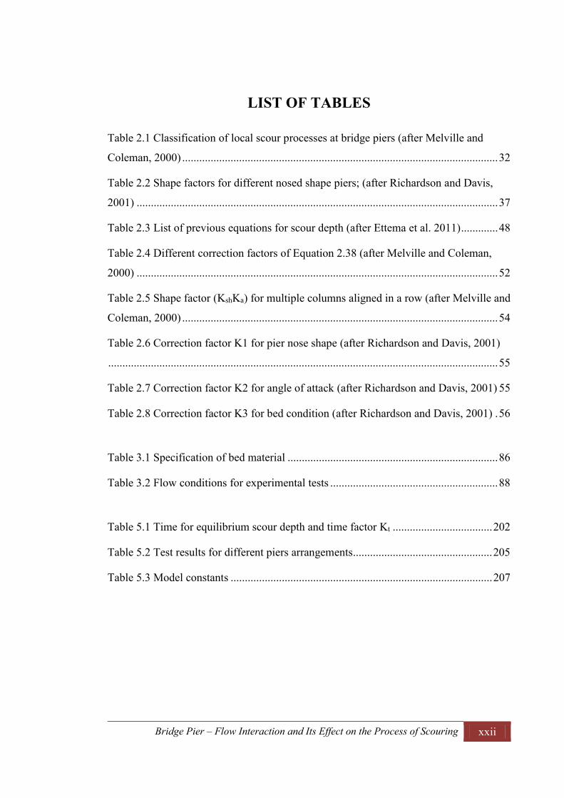
LIST OF TABLES
Table 2.1 Classification of local scour processes at bridge piers (after Melville and
Coleman, 2000) ............................................................................................................... 32
Table 2.2 Shape factors for different nosed shape piers; (after Richardson and Davis,
2001) ............................................................................................................................... 37
Table 2.3 List of previous equations for scour depth (after Ettema et al. 2011) ............. 48
Table 2.4 Different correction factors of Equation 2.38 (after Melville and Coleman,
2000) ............................................................................................................................... 52
Table 2.5 Shape factor (KshKa) for multiple columns aligned in a row (after Melville and
Coleman, 2000) ............................................................................................................... 54
Table 2.6 Correction factor K1 for pier nose shape (after Richardson and Davis, 2001)
......................................................................................................................................... 55
Table 2.7 Correction factor K2 for angle of attack (after Richardson and Davis, 2001) 55
Table 2.8 Correction factor K3 for bed condition (after Richardson and Davis, 2001) . 56
Table 3.1 Specification of bed material .......................................................................... 86
Table 3.2 Flow conditions for experimental tests ........................................................... 88
Table 5.1 Time for equilibrium scour depth and time factor Kt ................................... 202
Table 5.2 Test results for different piers arrangements................................................. 205
Table 5.3 Model constants ............................................................................................ 207

Bridge Pier – Flow Interaction and Its Effect on the Process of Scouring xxiii
LIST OF NOTATIONS
a = Edge of the bed layer at z=a
C′ = Chezy coefficient related to sediment grain
C1 = Column at upstream side (Column 1)
C2 = Column at downstream side (Column 2)
Cc = Coefficient of curvature
Cd = Drag coefficient
Cu = Coefficient of uniformity
c = Sediment concentration
D = Diameter of a pier
Dp = Projected width of a pier
d = Size of the sediment particle
d* = Dimensionless particle parameter
d1 = Equilibrium depth for single column bridge pier
d50 = Mean grain size of the sediment
ds = Depth of scour at any time
dse1 = Equilibrium depth of scour at Column 1
dse2 = Equilibrium depth of scour at Column 2
F = Dimensionless shape factor of sediment

Bridge Pier – Flow Interaction and Its Effect on the Process of Scouring xxiv
Fc = Coulomb force of resistance
Fd = Drag force
Fg = Submerged weight of a particle
Fr = Froude number
f = Frequency of vortex shedding
G = Parameter describing the effects of lateral distribution of flow in
the approach channel and the cross sectional shape of the approach
channel
g = Acceleration due to gravity
H = Hole size (threshold level for bursting process)
h
= Depth of flow
Ie = Sorting function for ejection event
Is = Sorting function for sweep event
KGmn = Correction factor proposed by Ataie-Ashtiani and Beheshti
(2006)
KI = Flow intensity parameter
Ks1 = Column-spacing factor for Column 1
Ks2 = Column-spacing factor for Column 2
Ksh = Shape parameter of a pier
Kt = Time factor for equilibrium scour depth
Kw = Adjustment factor for wide pier

Bridge Pier – Flow Interaction and Its Effect on the Process of Scouring xxv
Kα = Angle of flow attack parameter of a pier
ks = roughness height
L = Centre to centre distance between two columns
L′ = Length of the pier / Distance between two-column measured outer
to outer face of the columns.
m = Number of piles in line with flow as in Ataie-Ashtiani and
Beheshti (2006)
n = Number of piles normal to the flow as in Ataie-Ashtiani and
Beheshti (2006)
ne, nk = Dimensionless number to find the roughness height
Pi = Probability of occurrence of the events, where i = 1, 2, 3 and 4
Qi = Quadrant zones, where, i = 1, 2, 3 and 4
q = The rate of local scour in volume per unit time
q1 = The rate at which sediment is transported out from the scour hole
in volume per unit time
q2 = The rate at which sediment is supplied to the scour hole in volume
per unit time
qb = Rate of bed load transport
qb* = Dimensionless Einstein number to quantify bed load transport
qs = Rate of suspended load transport
R = Radius of the vortex
Re = Reynolds number
Rel = Reynolds number with respect to length of boundary layer

Bridge Pier – Flow Interaction and Its Effect on the Process of Scouring xxvi
S = Bed slope
Si = Stress fraction, where i = 1, 2, 3 and 4
St = Strouhal number
s = Specific gravity of the water
s′ = Submerged specific gravity of sediment particle
ss = Specific gravity of the sediment
T = Dimensionless transport stage parameter
TIu = Turbulence intensity component in stream-wise direction (x-
direction)
TIv = Turbulence intensity component in transverse direction (y-
direction)
TIw = Turbulence intensity component in vertical direction (z-direction)
TKE = Turbulence kinetic energy
te = Time to develop equilibrium scour depth
u = Velocity component in stream-wise direction (x-direction)
= Bed shear velocity
= Critical shear velocity
u′ = Fluctuating component of velocity in stream-wise direction (x-
direction)
V = Mean approach flow velocity
= Depth averaged velocity of fluid

Bridge Pier – Flow Interaction and Its Effect on the Process of Scouring xxvii
Va = Critical mean flow velocity for armour peak
Vc = Critical mean flow velocity for sediment entrainment
Vlp = Live bed peak velocity of flow
Vθ = Tangential vortex velocity = ω0R
v = Velocity component in transverse direction (y-direction)
v′ = Fluctuating component of velocity in transverse direction (y-
direction)
W = Width of the flume
w = Velocity component in vertical direction (z-direction)
w′ = Fluctuating component of velocity in vertical direction (z-
direction)
ws = Top width of the scour hole
x = Distance measured in stream-wise direction
y = Distance measured in transverse direction
Z, Z′ = Sediment number
z = Distance measured in vertical direction
= Vortex strength
δ = Thickness of boundary layer
μc = Coulomb friction coefficient
ν = Kinematic viscosity of fluid
ρ = Density of fluid

Bridge Pier – Flow Interaction and Its Effect on the Process of Scouring xxviii
ρs = Density of sediment material
σg = Geometric standard deviation of the sediment
= Bed shear stress
= Dimensionless critical shear stress parameter (Shields parameter)
= Critical shear stress
= Reynolds shear stress component in uv direction
= Reynolds shear stress component in uw direction
= Reynolds shear stress component in vv direction
ψ = Correction factor for stratification
ω0 = Angular velocity of revolution
Bridge Pier – Flow Interaction and Its Effect on the Process of Scouring 1
CHAPTER 1
INTRODUCTION
1.1 Background
1.2 Research Objectives
1.3 Scope and Limitation
1.4 Research Significance and Innovation
1.5 Research Methodology
1.6 Synopsis of Thesis
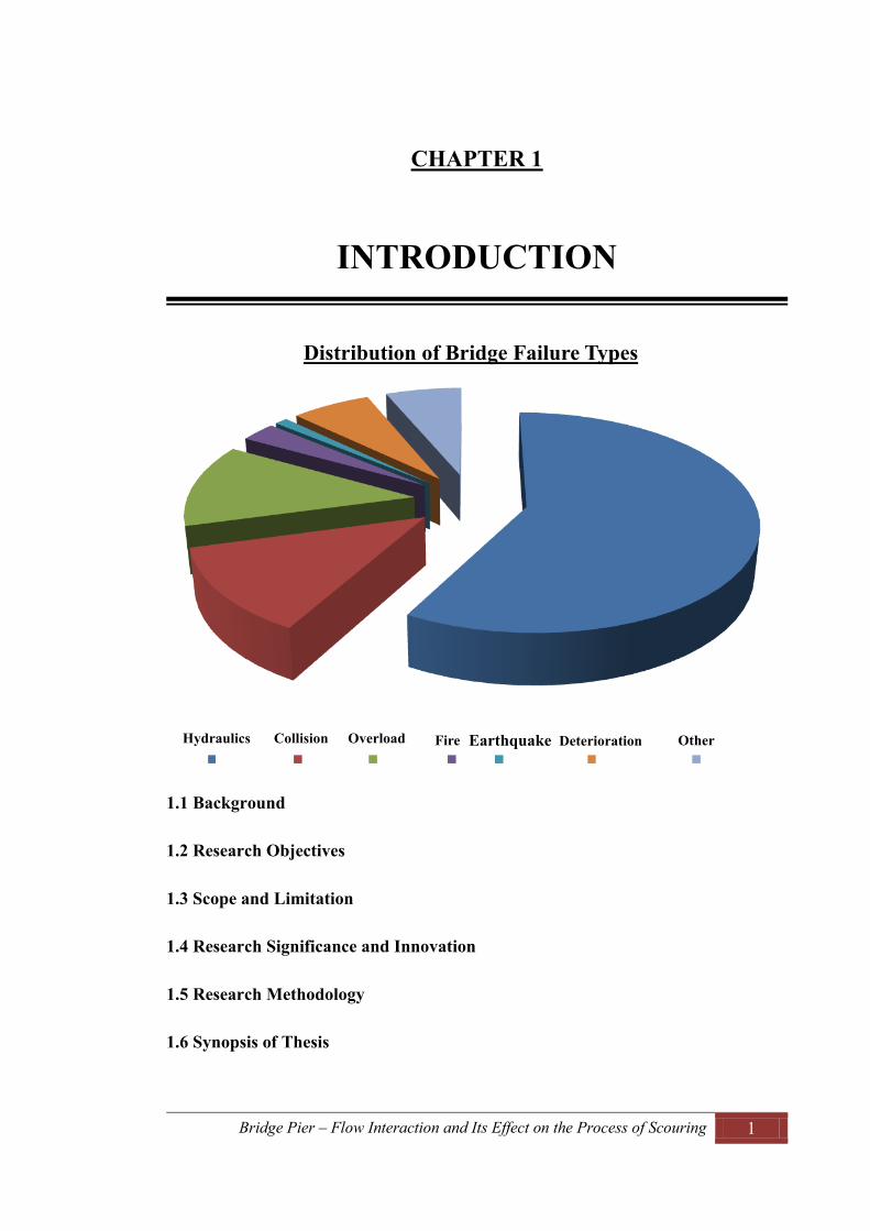
Distribution of Bridge Failure Types
Hydraulics Collision Overload Fire Earthquake Deterioration Other

Bridge Pier – Flow Interaction and Its Effect on the Process of Scouring 2
1. INTRODUCTION
1.1 Background
In the field of hydraulic engineering, the topic of river flow and the associated problems,
such as sediment transport, deformation of the riverbed, scouring and flooding are
considered as one of the major issues in the development of a country. Out of these issues,
deformation of the riverbed at the bridge site is a key area of interest to hydraulic
engineers and designers. According to Melville (1975), factors leading to the changes in
bed elevation at a bridge site are mainly classified in three different categories. Firstly
progressive aggradation and degradation of bed associated with a change in river regime;
secondly, temporary scour associated with changes in river stages, or with shifting of the
deep water channel; and thirdly, presence of hydraulic structure like bridge which
obstruct the flow resulting in the constriction of flow and hence scouring around bridge
piers or abutments.
In Australia, flood event has been reported as one of the main reasons of bridge failure.
According to the information provided on Wikipedia-contributors (2015), Fremantle
Railroad Bridge was collapsed in 1926 due to high flood event. In 2007, Gosford Culvert
was washed away due to flood events and five people were killed. The heavy flood event
in 2008 caused the Somerton Bridge was collapse. According to the recent study by
Pritchard (2013), Majority of Queensland area was declared as a natural disaster zone
because of the damaged caused by flooding. It was estimated that about 3 billion of the
damages were resulted from the flood events of 2011. Out of this amount, 5% of the cost
reflected to the bridge damage due to scour and piles undermine. Furthermore, it was
reported that, the post disaster recovery was adversely affected due to bridge damage.
In the history of bridge failure, scour around the bridge pier has been identified as the
main cause of failure. An analysis of 143 bridge failure incidents in different countries
during the period from 1961 to 1975 was carried out by Smith (1976). It was found that
about 70 bridges failed during floods of which about 45% could be attributed to the scour
around bridge piers. According to Melville (1992), out of 108 bridge failures observed in
New Zealand, between the period of 1960 and 1984, 29 were reported as failure due to
abutment scour. Furthermore Melville and Coleman (2000) reported that in New Zealand,

Bridge Pier – Flow Interaction and Its Effect on the Process of Scouring 3
at least one serious bridge failure each year can be attributed to the scour of the bridge
foundation.
As reported by many researchers for example Jones et al. (1995); Mueller (1997); Lagasse
and Richardson (2001); and Ameson et al. (2012); bridge scour is of significant concern
in the United States causing approximately 60 percent of all the U.S.A highway bridge
failures. Furthermore it was reported that in 1993 alone, more than 2500 bridges were
destroyed or severely damaged due to scour caused by severe flooding, which reflects
around $178 million of the total repair costs. Additionally, in 1994, over 1000 bridges
were reported closed in Georgia during flood, and the damage cost was estimated to be
around $130 million. There is a substantial amount of direct cost associated with repair
and replacement of river bridges damaged by flood. However, the indirect cost to local
businesses and industries due to disruption in commercial activities was estimated at more
than five times the direct repair cost. The high profile catastrophic collapse of the
Schoharie Creek Bridge in New York in 1987 in which 10 people died was caused by the
cumulative effect of pier scouring. It was reported by Mueller (1997) that in 1989,
according to Wardhana and Hadipriono (2003), more than 500 bridge failures in the
United States between 1989 and 2000 were studied and it was reported that the average
age of the failed bridges was 52.5 years (ranges from 1 year to 157 years).
According to an article reported by Novey (2013), the Colorado Department of
Transportation, CDOT estimated a minimum of 30 state highway bridges were destroyed
and 20 were seriously damaged by flood in the year 2013. Another article reported by KC
(2014), due to the degradation of the bed material, one of the main highway bridges over
the Tinau River in Nepal became deeper around the bridge pier by 1.5 m resulting in
exposure of the foundation of the bridge pier. Because of this, a very high risk of bridge
failure was reported. From the above review, it is justified to say that bridge scour is one
of the main bridge safety problems all over the world. The pictures presented in Figures
1.1 to 1.3 give clear illustration of scour problem around bridge piers and its
consequences as bridge failure.

Bridge Pier – Flow Interaction and Its Effect on the Process of Scouring 4
Figure 1.1 Bridge piers experiencing the flood events (USGS (2014)
Figure 1.2 a) Scour around bridge piers on the Logan river, Australia; (Queensland
Government (2013) ; and b) Scour around bridge piers on the Tinau river, Nepal,
(KC (2014)
a)
b)

Bridge Pier – Flow Interaction and Its Effect on the Process of Scouring 5
Figure 1.3 A bridge over the Gaula river in India washed away by flood in July 2008, (Bhatia (2013)
1.2 Research Objectives
The main objective of this study is to carry out an experimental investigation on three
dimensional flow structure and scour around the bridge piers comprising two circular
cylindrical columns in tandem arrangement. The effects of spacing between two columns
on flow structure and local scour around bridge pier are proposed to be study in depth.
In order to achieve this goal, the following specific objectives are proposed:
a) Deep understanding of the flow structure concept and the scour mechanism for
local scour around bridge piers such as horseshoe vortex, vortex shedding, vortex
strength, vortex shedding frequency and shear velocity
b) Detailed study of interaction of turbulence (coherent structures, bursting
phenomenon, Reynolds shear stresses, turbulence intensity, turbulent kinetic
energy, flow field, etc.) and the bridge piers.
c) Assessing and analysing the suggested equations to predict the local scour depth
around bridge piers and to determine the important factors affecting the local
scour around a bridge pier
d) Conducting detailed experimental studies on the flow structure and local scour
around bridge piers using a single column and two column bridge piers with
different column spacing arrangement
e) Determination and evaluation of temporal variation of the local scour depth
around bridge piers with a single and two columns based on the experimental data

Bridge Pier – Flow Interaction and Its Effect on the Process of Scouring 6
f) Comparison of single-column and twin-column bridge piers effects on the flow
structure and local scour around the piers based on the results obtained from the
experimental studies Analysing the experimental results to obtain deep
knowledge on the influence of the bridge piers interaction on the flow structure
and scour around the bridge piers
g) Suggesting a design method to predict the scour depth around bridge piers with
two columns in tandem arrangements
h) Comparing the results of experimental studies with the well-known scour depth
prediction equations as well as a number of common definitions of equilibrium
scour depth available from past studies
1.3 Scope and Limitation of Research
Due to the complex nature of flow around bridge piers and various uncertainties on
different parameters affecting the scour depth, laboratory based experimental study is the
widely adopted method for achieving precise and reliable results. Hence the present study
is aimed to carry out an experimental investigation. However, there are some limitations
on experimental setup and the parameters given as under:
a) Cohesion-less and uniformly graded sand as bed material was used for all the
experiments.
b) It was considered that there is occurrence of local scour around bridge piers under
the clear water flow condition.
c) Only a cylindrical pier model with a circular cross-section was used
d) The bridge piers comprising maximum number of two circular cylindrical
columns were adopted throughout the research work.
e) The columns of a bridge pier were installed in a tandem arrangement i.e. angle of
flow attack is zero.
1.4 Research Significance and Innovation
Numerous studies have been carried out since the late 1950s on the flow structure and
scour around bridge piers. However, problems in understanding the complicated flow and
scouring mechanism remain challenging. Although numerous scour depth prediction
Bridge Pier – Flow Interaction and Its Effect on the Process of Scouring 7
equations have been suggested by many investigators, almost all of them are developed
based on a single pier arrangement. In contrast to vast amount of investigations carried
out for the flow around a single pier, there are limited studies on flow around a group of
piers. The flow around piers comprising a multiple in-line columns is not well
investigated. However, in practice, bridge piers often comprise a number of circular
columns aligned in the flow direction that together support the loading of the structure.
Thus, a detailed study on flow around bridge piers with two in-line columns is studied
experimentally in this research.
The present study aims to provide a notable contribution to the body of knowledge
through the following innovations:
a) Studying the three dimensional flow structure around the bridge piers with single
and two columns using physical-hydraulic models in the laboratory
b) Investigation of the interaction of bridge piers on the flow structure and scouring
process around the bridge piers using two-column bridge piers model aligned in
a line with different spacing between them
c) Suggesting a design relationship to predict the local scour depth around bridge
piers with two columns in tandem arrangements
d) Employing advanced measurement techniques to capture accurate results
1.5 Research Methodology
The present study is primarily based on the laboratory experiments consisting of
measuring instantaneous three dimensional velocity components, experimental
investigation of temporal variation of scour depth around single and two columned bridge
piers and analysis of equilibrium scour depth under various flow conditions and columns
arrangements. The following conditions and parameters have been established for all the
experimental work:
a) Steady state approach flow with clear water scour condition was applied.
b) The model bridge piers comprising single and two cylindrical columns with
circular cross-sections were used in all experiments. For the two-column case,
they were installed in tandem arrangements with different spacing between them.

Bridge Pier – Flow Interaction and Its Effect on the Process of Scouring 8
All the experiments related to flow structures were carried out under flatbed condition
establishing the rough bed surface using sand as the bed material. Instantaneous three
dimensional velocity components were measured using Acoustic Doppler Velocimetry
(ADV). The ADV measurements were carried out in different horizontal planes.
Additionally the experiments on flow around bridge piers in different vertical planes were
carried out using Particle Image Velocimetry (PIV) method. In the PIV method, a series
of instantaneous images were captured and analysed to get the two dimensional velocity
components. To measure the scour depth and the final bed profile, a vernier depth gauge
with the least count of 0.1 mm was used.
The measured data were analysed and the results were presented in graphical form using
profile and contour plots. Furthermore, the results were compared with the results from
the previous investigations.
1.6 Synopsis of Thesis
This thesis contains altogether seven chapters. A brief outline of each chapter is as
follows:
In Chapter 1, general background of bridge scour and associated problems are presented.
Additionally, this chapter presents the objectives of the study, limitation, research
significance and innovation, and methodology.
Chapter 2 is mainly focused on the compilation of existing knowledge in the field of
bridge scour and identification of the scientific gap that needs to be fulfilled to achieve
the objectives of this research. A synthetic review on the scour at bridge crossing is
presented which is followed by local scour around bridge piers, mechanism of local scour
and analysis of pier scour. Moreover, review on flow regime around bridge piers,
temporal development of scour depth and various methods of prediction of local scour
depth are presented in this chapter. In addition to this, theoretical development of open
channel flow and sediment transport are presented. This chapter consists of governing
equations of flow in open channel and theory of turbulence structures in open channel
flow. It also summaries the basic concept of sediment transport providing the various
relations related to various forms of sediment transport.

Bridge Pier – Flow Interaction and Its Effect on the Process of Scouring 9
Chapter 3 gives a detailed description of facilities and equipment used for the
experimental tests. In addition, design of the physical model, advance measurement
techniques employed in the experiments and experimental procedures for this study are
described in this chapter.
Chapter 4 and 5 provide the results obtained from the laboratory experiments on flow
structures and scour around bridge piers. The various test results from single column and
two column experiments are analyzed and compared in order to work out the effect of
spacing between two columns on flow structures and scour around bridge piers.
Finally, conclusions from this study and recommendations for future research are
provided in Chapter 6, followed by References and Appendices containing the detailed
figures of experimental results.

Bridge Pier – Flow Interaction and Its Effect on the Process of Scouring 10
CHAPTER 2
LITERATURE REVIEW
2.1 Introduction
2.2 Scour at Bridge Crossings
2.3 Sediment Transport and Local Scour around Bridge Piers
2.4 Open Channel Flow and Flow around Bridge Piers
2.5 Summary and Identification of the Gap in Literature
624 – 546 BCThe Greek Thales, often described as theworld's first scientist, declared water asubstance rather than a mystic gift fromthe gods, thus paving the way for futureresearch into water, and probably muchirritating the local priesthood at the sametime.(http://www.tiefenbach-waterhydraulics.com/waterhydraulics/historyofwaterhydraulics.html)

Bridge Pier – Flow Interaction and Its Effect on the Process of Scouring 11
2. LITERATURE REVIEW
2.1 Introduction
In the past decades, a number of studies have been carried out in the field of scour around
bridge piers. Based on the previous investigations available in literature, this chapter
summarises the basic concepts of scour around bridge piers. This explanation is followed
by a description of different types of scour, factors that contribute in the process of
scouring and description of the flow field around the pier. A comprehensive review on
some previous studies on scour around bridge piers is also presented in this chapter.
2.2 Scour at Bridge Crossings
Scour is a phenomenon of sediment removal from around a hydraulic structure due to
interaction between flow and the hydraulic structure such as bridge piers placed in
flowing water. Breusers et al. (1977) defined scour as a consequence of the erosive action
of flowing water, which removes and erodes materials from the bed and banks of streams
and also from the vicinity of bridge piers and abutments. According to Melville and
Coleman (2000) scour is defined as lowering the riverbed by water erosion such that there
is a tendency to expose the foundations of a bridge. In this definition, it is assumed that
the level of the riverbed prior to the commencement of the scour is the natural bed level
and the amount of reduction below the natural bed level is termed as the scour depth.
Figure 2.1 Types of scour at a bridge, (after Melville and Coleman, 2000)

Bridge Pier – Flow Interaction and Its Effect on the Process of Scouring 12
Cheremisinoff et al. (1987) stated that scour can either be caused by normal flows or flood
events. During a flood event, the rate of scouring is more than that in a normal flow
condition because of the higher flow velocity. The different components of scour are
clearly shown in Figure 2.1. Richardson and Davis (2001) explained that the total scour
at a highway crossing is comprised of three components namely long term aggradation
and degradation, general scour and local scour. Furthermore, Melville and Coleman
(2000) suggested that various types of scour that can occur at a bridge crossing are
typically referred to: general scour, contraction scour and local scour. A summarised form
of scour types is shown in Figure 2.2.
Figure 2.2 Classification of scour (after Melville and Coleman, 2000)
2.2.1 General Scour
According to Melville and Coleman (2000), general scour deals with the changes in river
bed due to natural or human induced causes. Because of the general scour, overall
longitudinal profile of the river channel is lowered. It occurs through a change in the flow
regime in the river system resulting in general degradation of the bed level. General scour
occurs irrespective of the existence of the bridge; and it can occur as either long-term
scour or short-term scour. Short-term scour is because of a single flood or several closely
spaced floods. On the other hand, long-term scour has a considerably extensive time scale
(i.e. several years longer), and it includes progressive degradation and lateral bank
erosion.

Bridge Pier – Flow Interaction and Its Effect on the Process of Scouring 13
2.2.2 Localised Scour
As suggested by Melville and Coleman (2000), localised scour is a collective term of
contraction scour and local scour, and they are directly attributable to the existence of the
bridge. When the river flow approaches the bridge, it usually converges causing a
constriction of flow. Because of this contraction, the flow accelerates to the narrowest
section (vena contracta). The flow then decelerates and the live river expands beyond the
vena contracta to defuse gradually into the full downstream width of the channel. The
accelerated flow induces scour across the contracted section. This scour is referred to as
contraction scour. On the other hand, when the flow approaches hydraulic structures such
as bridge piers, abutments, spurs and embankments, there is a formation of interference
between structures and the flow. This also causes acceleration of the flow around the
structures resulting in removal of material from around piers, abutments, spurs and
embankments. This scour is termed local scour, which is clearly illustrated in the
photograph shown in Figure 2.3.
Figure 2.3 Local scour at bridge piers; (Vasquz, 2006)
2.3 Sediment Transport and Local Scour around Bridge Piers
2.3.1 Basics of Sediment Transport
The fragmental material formed by the physical and chemical disintegration of rocks is
known as sediment. The size of the sediment varies from the large boulder to colloidal
Bridge Pier – Flow Interaction and Its Effect on the Process of Scouring 14
size of fragments with a variety of shapes. Once the sediment particles are detached from
their original source, they may either be transported by gravity, wind or water. Usually
the sediments can be transported in three different modes of particle motion namely:
rolling or sliding particle motion; saltation or hopping particle motion; and suspended
particle motion.
When the value of shear velocity at the bed just exceeds the critical value, the bed material
will start rolling or sliding in continuous contact with the bed. Further increasing the value
of bed shear velocity, the particle will be moving along the bed by more or less regular
jumps, which are called sediment transport by saltation. The transport of sediment
particles by rolling and saltation is called bed load transport. As the bed shear velocity
exceeds the fall velocity of the particles, there is lifting of sediment particles; as a result
the particles may go into suspension. The transport of sediment particles in this way is
called suspended load transport.
2.3.1.1 Threshold of Sediment Motion
Melville (1975) presented the definition of threshold of motion or critical condition as
given in Sedimentation Manual published in 1966. It states that ‟when the hydrodynamic
force acting on a grain of sediment has reached a value that, if increased even slightly
will put the grain into motion, critical or threshold conditions are said to have been
reached.” According to Chaudhry (2007), the drag force exerted on sediment particles on
the riverbed is the main factor for initiating the sediment motion. For the initiation of
sediment motion the applied drag force must exceed a threshold value. The resistance to
motion is due to cohesion in the case of clay-rich sediment and from the Coulomb friction
in the case of non-cohesive sediment. As shown in Figure 2.4, a simplified case of
sediment motion, for a small bed slope, such that S 1, consider that the roughness height,
ks = nkd50, where nk is a dimensionless number and d50 is the mean size of the sediment
particles. Consider an exposed particle protrudes up from the mean bed level by an
amount ned50, where ne is again a dimensionless number. If the flow is turbulent, then the
drag force, Fd and the submerged weight of the particle, Fg, is given by

Bridge Pier – Flow Interaction and Its Effect on the Process of Scouring 15
2.1
2.2
where is the fluid density, s′ = (ss - s), is the submerged specific gravity of sediment
particle, g is the acceleration due to gravity and V is the fluid velocity at the level of
particle, Cd is the drag coefficient. The Coulomb resistive force Fc is given by
2.3
where, is the Coulomb friction coefficient. At threshold condition of sediment motion,
Equations 2.1 and 2.3 give
2.4
Figure 2.4 Threshold condition for the sediment entrainment

Bridge Pier – Flow Interaction and Its Effect on the Process of Scouring 16
The expression for the velocity distribution over a rough boundary surface is given by:
2.5
Substituting the value of V from Equation 2.5 to Equation 2.4, gives
2.6
In Equation 2.6 the term is known as the bed shear stress. In order to entrain the
sediment particle, the non-dimensional bed shear stress must exceed .
Melville and Coleman (2000) described that the Shields diagram can be used to evaluate
threshold flow conditions for the motion of a given sediment. The Shields diagram
indicates that the condition of the movement of bed material can be identified by using
dimensionless critical shear stress under observed temperature, specific gravity and mean
size of sediment material which is known as Shield’s parameter and is expressed as:
2.7
where,
= dimensionless critical shear stress parameter (Shields parameter)
= bed shear stress
ss = specific gravity of sediment material
s = specific gravity of water
g = acceleration due to gravity
d50 = mean grain size of sediment
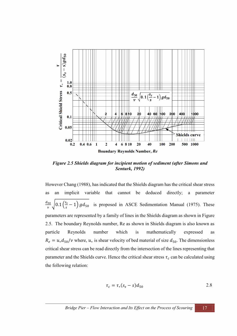
Bridge Pier – Flow Interaction and Its Effect on the Process of Scouring 17
Figure 2.5 Shields diagram for incipient motion of sediment (after Simons and
Senturk, 1992)
However Chang (1988), has indicated that the Shields diagram has the critical shear stress
as an implicit variable that cannot be deduced directly; a parameter
is proposed in ASCE Sedimentation Manual (1975). These
parameters are represented by a family of lines in the Shields diagram as shown in Figure
2.5. The boundary Reynolds number, Re as shown in Shields diagram is also known as
particle Reynolds number which is mathematically expressed as
where, is shear velocity of bed material of size . The dimensionless
critical shear stress can be read directly from the intersection of the lines representing that
parameter and the Shields curve. Hence the critical shear stress can be calculated using
the following relation:
2.8

Bridge Pier – Flow Interaction and Its Effect on the Process of Scouring 18
The value of critical shear stress can be used to calculate the critical shear velocity of the
Inflow using the following relation:
where,
= critical shear velocity
= density of water
According to Melville and Coleman (2000), critical shear velocity, for quartz material
in water at 20o C, as shown in Figure 2.6 can be alternatively calculated using the
following equations which is only based on the mean grain size of the sediment material:
For 0.1 mm < d50 < 1 mm,
Figure 2.6 Shear velocity chart for quartz sediment in water at 20° C; (after Melville
and Coleman, 2000)
2.9
2.10 For 1 mm < d50 < 100 mm,
2.11
Bridge Pier – Flow Interaction and Its Effect on the Process of Scouring 19
If critical mean velocity of flow, Vc, is preferred to describe threshold motion of the
sediment, it can be determined using the following relation given by Melville and
Coleman (2000):
where,
= critical mean velocity of flow
= depth of flow
Melville and Coleman (2000), further reported that the critical mean velocity of flow can
be alternatively calculated using an empirical relation given by Neil (1968):
2.3.1.2 Bed Load Transport
According to Van Rijn (1984a) bed load transport is defined as the transport of sediment
particles by rolling and saltating along the bed surface. Another definition by Einstein
(1950) states that it is the movement of the particles by rolling, sliding, and, sometimes
by jumping in the bed layer which has the thickness of 2 grain diameters immediately
above the bed. Van Rijn (1984a) has given a method to calculate the bed load transport
rate which is given as
2.14
2.12
2.13
Bridge Pier – Flow Interaction and Its Effect on the Process of Scouring 20
where is the bed load transport rate (in m2/s), s is the specific gravity of sediment,
is the particle parameter and T is the transport stage parameter. The particle parameter,
, and the transport stage parameter, T, are given by the following equations:
2.15
2.16
in which, g is the acceleration due to gravity, ν is the kinematic viscosity, is the bed
shear velocity related to sediment and is the Shields critical bed shear velocity. If V
is the mean flow velocity and C′ is Chezy-coefficient related to grains then the bed shear
velocity related to sediment, is given by
2.17
As reported by Chaudhry (2007), bed load transport can be quantified using an empirical
relation of non-dimensional Einstein number, , which is given by
2.18
Some popular bed load transport relations based on Shields stresses for well graded sediments are reported by Chaudhry (2007) which are given as under:
1. Meyer-Peter and Muller relation
; 2.19
2. Wong and Parker – correction of Meyer-Peter and Muller relation

Bridge Pier – Flow Interaction and Its Effect on the Process of Scouring 21
; 2.20
3. Einstein equation
2.21
4. Parker equation- fit to Einstein equation
; 2.22
5. Ashida and Michiue relation
; 2.23
6. Engelund and Fredsoe relation
; 2.24
2.3.1.3 Suspended Load Transport
Bagnold (1966) defined the suspended load transport as the process in which the excess
weight of the particles is supported by upward impulses of turbulent eddies. He further
gave the condition of initiation of suspension, which states that when the value of bed
shear velocity exceeds the particle fall velocity, suspension will occur. According to Van
Rijn (1984b), suspension will start at considerably smaller bed-shear velocities. When the
bed shear velocity is greater than the fall velocity of the particles, they can be lifted up to
a level at which the upward turbulent force is higher than the submerged weight of
sediment particle. This keeps the particles in suspension mode. He further reported that
the behaviour of suspended sediment particles can be is described in terms of sediment
concentration. The suspended sediment concentration decreases with the distance from
the bed, the rate of which depends on the ratio of the fall velocity and the bed shear
velocity.

Bridge Pier – Flow Interaction and Its Effect on the Process of Scouring 22
According to Van Rijn (1993) the rate of suspended load transport can be calculated by
integrating the product of velocity and sediment concentration from the edge of the bed
layer (z=a) to the water surface (z=h) as shown in Figure 2.7.
2.25
or
2.26
with
2.27
where is the suspended load transport rate, V is the fluid velocity at height z above bed,
c is the sediment concentration at height z from bed, is the depth averaged fluid
velocity, is the sediment concentration at height z=a above bed, h is the depth of flow,
and F is the dimensionless shape factor (as in Van Rijn, 1984).
Figure 2.7 Definition sketch of suspended load transport; (after Van Rijn, 1993)
The parameters used in Equation 2.27 can be determined using the following relations:
Sediment concentration at height (z=a) is given by

Bridge Pier – Flow Interaction and Its Effect on the Process of Scouring 23
2.28
In Equation 2.28, the values of the dimensionless parameter, , and dimensionless
transport stage parameter, T, can be computed using Equations 2.15 and 2.16,
respectively.
Dimensionless shape factor, F, for 0.3 ≤ Z′ ≤ 3 and 0.01 ≤ a/h ≤ 0.1 is given by:
2.29
where Z′ = Z +ψ is the suspension number with correction factor for stratification ψ. The
shape factor, F, for a/h = 0.01, 0.05 and 0.1 can be determined using Figure 2.8.
Figure 2.8 Shape factor for different suspension numbers; (after Van Rijn, 1993)

Bridge Pier – Flow Interaction and Its Effect on the Process of Scouring 24
2.3.2 Local Scour around Bridge Piers Melville (1975) suggested that the local scour can be classified according to the amount
of bed material supplied into the scour area and the capacity of transport out of the scour
area. The rate of scour hole in volume per unit time is expressed as the difference between
the amount of sediment supplied in and transported out of the scour hole, which is
expressed in the following equation:
2.30 where,
= the rate of local scour in volume per unit time
= the rate at which sediment is transported out from the scour hole in volume per unit time
= the rate at which sediment is supplied to the scour hole in volume per unit time
This leads to an identification of two types of local scour:
Clear Water Scour
Clear water scour occurs when there is no movement of bed material in the flow upstream
of the crossing. This condition of scour is just because of the obstructions (piers,
abutments) in the flow that accelerate the flow and create vortices around the obstructions
cause bed material around them to move. In Equation 2.30, the rate of sediment supply
to the scour hole is equal to zero ( = 0) for clear water scour condition. In this case, the
depth of scour hole continues to grow until the equilibrium scour depth is reached
Live-bed Scour
Live bed scour occurs when there is transport of bed material from upstream reach into
the crossing. In live bed local scour, the scour hole is continuously supplied with the
sediment transported from upstream reach. In this case the rates of sediment transport to
and from the scour hole are greater than zero (i.e. , > 0). Equilibrium scour depth is
reached when the rate of sediment supply to the scour hole is equal to the rate of sediment
transported out of the scour hole (i.e. = ).

Bridge Pier – Flow Interaction and Its Effect on the Process of Scouring 25
Figure 2.9 shows the two types of scour and the equilibrium scour depth, in which the
depth of the scour is presented as a function of time. It is clear from the figure that the
equilibrium scour depth for clear water scour is approached asymptotically while for the
live bed scour, there are non-periodic oscillations about equilibrium scour depth.
Additionally it can be seen that the equilibrium scour depth for clear water scour is about
10% greater than that for live bed scour. According to the citation made by Melville
(1975), the time development of local scouring is governed by an exponential law.
Figure 2.9 Local scour around bridge piers as a function of time; (after Richardson and Davis, 2001)
Carsten (1966) defined a sediment number, based on sediment size and the mean velocity
of flow at which local scour begins. According to his definition, the sediment number is
given by Equation 2.31.
2.31
where,
Z = sediment number
V = mean velocity of the undisturbed flow
ss = the specific gravity of the sediment

Bridge Pier – Flow Interaction and Its Effect on the Process of Scouring 26
g = acceleration due to gravity
d = mean grain diameter of the sediment
Furthermore Carsten (1966) defined two types of sediment numbers at which local scour
begins and continuous sediment transport occurs, which are denoted by Nsc1 and Nsc2,
respectively. Additionally, he stated that “for irrotational flow, the velocity at the sides of
the pier is twice the approach velocity. Therefore, a reasonable approximation is that Zsc1
= Zsc2/2”. For the localized scour, the sediment number ranges from 1.12 to 2.24,
corresponding to Nsc1 and Nsc2, respectively.
2.3.3 Mechanism of Local Scour
Many researchers (Melville (1975); Ettema (1980); Qadar (1981); Chiew (1984);
Davoren (1985); Hamill (1999); Melville and Coleman (2000); Richardson and Davis
(2001); Sheppard (2004); (2005) in the past have believed that the basic mechanism of
local scour is a system of vortices developed around bridge piers. Figure 2.10 shows the
different components of flow field contributing to the scour around bridge piers.
Melville (1975) reported that the system of vortices (horseshoe vortex and wake vortex)
developed around the bridge pier is the primary cause of the scour around the bridge pier.
The horseshoe vortex increases the velocities near the bed, which results in an increase
in sediment transport capacity of the flow. The wake vortex system keeps the sediment
suspended condition and also acts as a ‘vacuum cleaner’ and the bed material is carried
to downstream side by the eddies shaded from the pier.
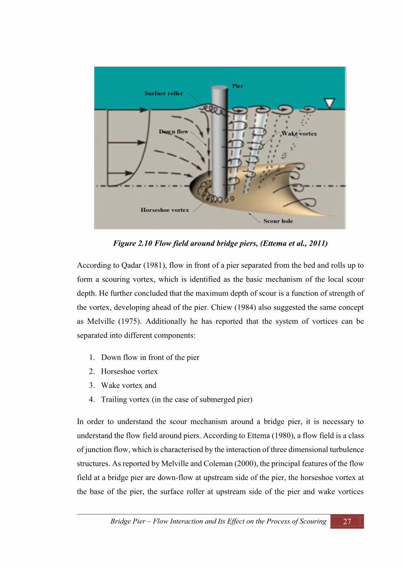
Bridge Pier – Flow Interaction and Its Effect on the Process of Scouring 27
Figure 2.10 Flow field around bridge piers, (Ettema et al., 2011)
According to Qadar (1981), flow in front of a pier separated from the bed and rolls up to
form a scouring vortex, which is identified as the basic mechanism of the local scour
depth. He further concluded that the maximum depth of scour is a function of strength of
the vortex, developing ahead of the pier. Chiew (1984) also suggested the same concept
as Melville (1975). Additionally he has reported that the system of vortices can be
separated into different components:
1. Down flow in front of the pier
2. Horseshoe vortex
3. Wake vortex and
4. Trailing vortex (in the case of submerged pier)
In order to understand the scour mechanism around a bridge pier, it is necessary to
understand the flow field around piers. According to Ettema (1980), a flow field is a class
of junction flow, which is characterised by the interaction of three dimensional turbulence
structures. As reported by Melville and Coleman (2000), the principal features of the flow
field at a bridge pier are down-flow at upstream side of the pier, the horseshoe vortex at
the base of the pier, the surface roller at upstream side of the pier and wake vortices

Bridge Pier – Flow Interaction and Its Effect on the Process of Scouring 28
downstream of the pier. Ettema et al. (2011) suggested three categories of pier flow field,
depending on the width of the pier (D) and the depth of flow (h).
1. Narrow piers (h/D > 1.4)
2. Transitional piers (0.2<h/D<1.4)
3. Wide piers (h/D <0.2)
The main features of flow field at narrow piers can easily be comprehended when
considering a single column pier, installed in a relatively deep, wide channel as shown in
Figure 2.10. In this type of pier, the scour is deepest at the pier face. Ettema et al. (2011)
reported that the flow field at narrow piers consists of an interacting and unsteady set of
flow features including, flow impact against the pier face producing down-flow and up-
flow with rollers; flow converging, contracting then diverging; the generation, transport
and dissipation of a large scale turbulence structure at the base of the pier foundation
junction; detaching shear layer at each pier flank; and, wake vortices convected through
the pier’s wake. For the transition piers, there exists almost the same flow field as for
narrow piers. However, the flow field (specially the down-flow) begins to alter in
response to the reduction of the depth of flow or increase in the size of the pier. For wide
piers, as the flow approaches the pier, it turns and flows laterally along the pier face before
contracting and passing around the side of the pier. The weak down-flow is developed,
causing less scouring at the centre of the pier in the upstream side. The wide pier increases
flow blockage, which modifies the lateral distribution of approach flow over a longer
distance upstream of a pier.
As flow approaches a pier, it decelerates and impinges against the pier’s centreline. The
flow comes to rest and the stagnation pressure on the upstream face of the pier attains a
maximum near the level where the flow impinges. Hence, there is generation of a
downward pressure gradient along the pier’s leading face that causes the down-flow with
a fully turbulent shear flow. In addition to this, the flow contracts as it pass around the
sides of the pier with increase in flow velocity and bed shear stress. Hence, in most cases,
the scour begins at the side of a pier and the high velocity washes the excavated bed
materials to the downstream side. Melville (1975) concluded from his experiments that
there was a strong vertical down-flow developed ahead of the cylinder as the scour hole

Bridge Pier – Flow Interaction and Its Effect on the Process of Scouring 29
enlarged. He further noticed that the strength of the horseshoe vortex increased rapidly
and the velocity near the bottom of the hole decreased as the scour hole was enlarged.
Further increase in the scour hole results in the decrease in the vortex strength and reaches
a constant value at the equilibrium stage. There is also an up-flow at the level of impinge,
which interacts with the free water surface forming a surface roller and hence there is a
rise in the water surface at the upstream side of the pier. The rise in the water surface
depends on the approach velocity and the shape of the pier.
It was reported in the (2005) that the wake vortex system is also an important mechanism
of scour around bridge piers. Wake vortices are developed due to flow separation on the
bridge pier. Strong wake vortices may develop a large scour hole downstream from the
piers. The vertical component of the flow at the wake put the bed material in suspension
although there is a very weak streamwise and transverse component of velocity.
According to Sheppard (2004), the scour mechanism at the bridge pier also depends on
the ratio of pier width to the sediment grain size, D/d50. This mechanism results from the
pressure gradient field generated by the presence of a structure such as a bridge pier in
the flow. The pressure gradients impose pressure force on the sediment grains that can be
much greater than the drag force due to the flow around the grains. The force due to this
pressure gradient decreased with increase in the value of D/d50.
2.3.4 Parameters for Analysis of Pier Scour
The local scour depth around bridge piers depends on various parameters, which are
basically categorized in four different groups comprising the flow parameter, the bed
sediment parameter, the pier geometry parameter and time. According to Melville and
Coleman (2000), local scour can be defined as a function of the above mentioned
parameters, which can be written as:
where,
= density of fluid
2.32
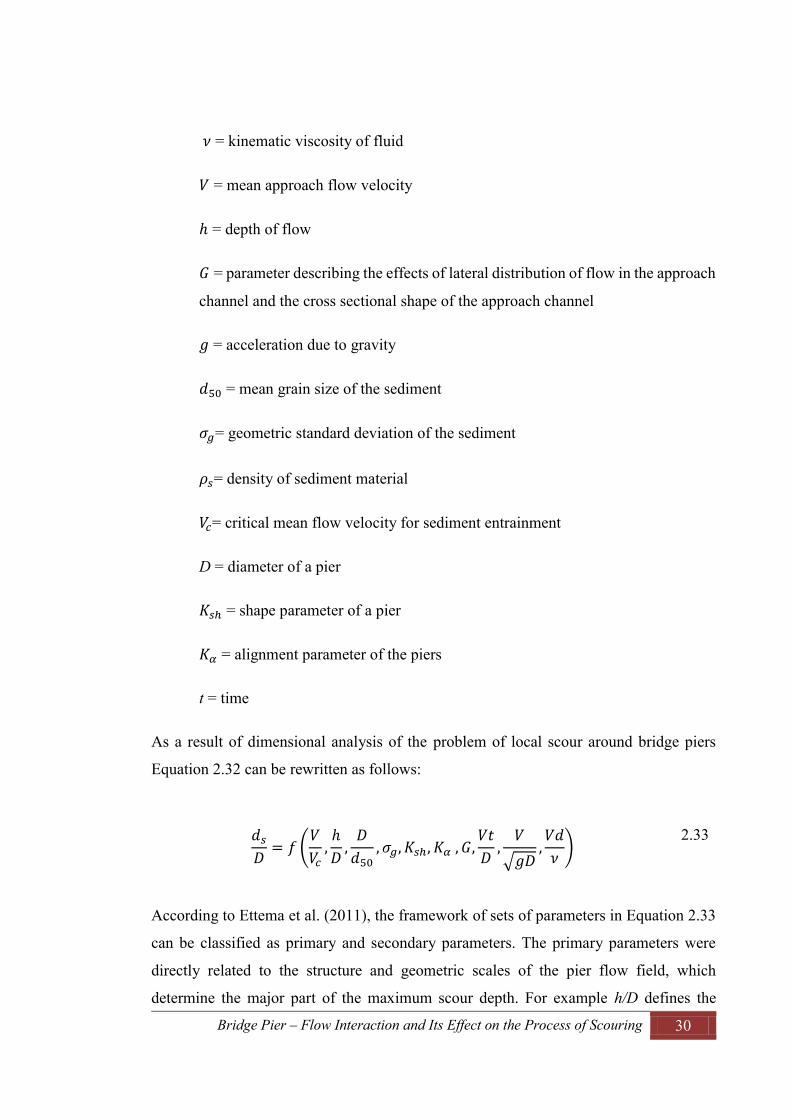
Bridge Pier – Flow Interaction and Its Effect on the Process of Scouring 30
= kinematic viscosity of fluid
= mean approach flow velocity
= depth of flow
= parameter describing the effects of lateral distribution of flow in the approach
channel and the cross sectional shape of the approach channel
= acceleration due to gravity
= mean grain size of the sediment
= geometric standard deviation of the sediment
= density of sediment material
= critical mean flow velocity for sediment entrainment
D = diameter of a pier
= shape parameter of a pier
= alignment parameter of the piers
t = time
As a result of dimensional analysis of the problem of local scour around bridge piers
Equation 2.32 can be rewritten as follows:
According to Ettema et al. (2011), the framework of sets of parameters in Equation 2.33
can be classified as primary and secondary parameters. The primary parameters were
directly related to the structure and geometric scales of the pier flow field, which
determine the major part of the maximum scour depth. For example h/D defines the
2.33

Bridge Pier – Flow Interaction and Its Effect on the Process of Scouring 31
geometric scale of the pier flow field in a vertical plane parallel and perpendicular to the
streamwise and the transverse direction, respectively; D/d50 is related to the length scale
of pier width and mean grain size of bed material; and indicate the pier shape and
angle of flow attack parameters. On the other hand, the magnitudes of secondary
parameters are prescribed by the primary parameters described above. , , and
are the secondary parameters in which, Vc is prescribed by d50 , Euler number is
related to the inertial force due to vortices. The term is the pier Reynolds number,
which accounts for the vortex shedding behind the pier. The parameter characterizes
the temporal development of scour associated with flow field and the foundation material.
Detailed description of these parameters and their effects on the scour around bridge piers
are presented in Section 2.3.5.
2.3.5 Factors Affecting the Local Scour at Bridge Site
Extensive investigations have been carried out for studying the factors affecting the local
scour depth around bridge piers by many researchers, such as Laursen and Toch (1953);
Ettema (1980); Raudkivi and Ettema (1983); Chiew (1984); Melville and Sutherland
(1988); Yanmaz and Altinbilek (1991); Melville and Coleman (2000); and Ettema et al.
(2011). According to Ettema et al. (2011), most of the studies have aimed to describe the
influences of different parameters on the scour around bridge piers, although still there
are significant gaps in overall understanding of the scour mechanism and the scour depth
prediction. This may be due to the difficulties in conducting laboratory flume experiments
on large geometric scales or insufficiency of reliable field data. Melville and Coleman
(2000) provided comprehensive publications explaining the factors affecting the scour at
bridge piers. They used laboratory data to assess the influence of each parameter as
presented in Equation 2.33.
2.3.5.1 Effect of Flow Shallowness, h/D
According to Raudkivi (1998), the scour depth is independent of the depth of flow when
it is greater than three times the pier diameter. He further reported that decrease in flow
depth results in increase in the surface roller (bow wave) which interacts with the down-
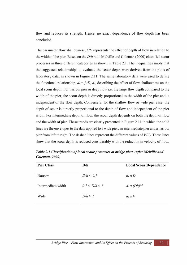
Bridge Pier – Flow Interaction and Its Effect on the Process of Scouring 32
flow and reduces its strength. Hence, no exact dependence of flow depth has been
concluded.
The parameter flow shallowness, h/D represents the effect of depth of flow in relation to
the width of the pier. Based on the D/h ratio Melville and Coleman (2000) classified scour
processes in three different categories as shown in Table 2.1. The inequalities imply that
the suggested relationships to evaluate the scour depth were derived from the plots of
laboratory data, as shown in Figure 2.11. The same laboratory data were used to define
the functional relationship, ds = f (D, h), describing the effect of flow shallowness on the
local scour depth. For narrow pier or deep flow i.e. the large flow depth compared to the
width of the pier, the scour depth is directly proportional to the width of the pier and is
independent of the flow depth. Conversely, for the shallow flow or wide pier case, the
depth of scour is directly proportional to the depth of flow and independent of the pier
width. For intermediate depth of flow, the scour depth depends on both the depth of flow
and the width of pier. These trends are clearly presented in Figure 2.11 in which the solid
lines are the envelopes to the data applied to a wide pier, an intermediate pier and a narrow
pier from left to right. The dashed lines represent the different values of V/Vc. These lines
show that the scour depth is reduced considerably with the reduction in velocity of flow.
Table 2.1 Classification of local scour processes at bridge piers (after Melville and Coleman, 2000)
Pier Class D/h Local Scour Dependence
Narrow D/h < 0.7 ds α D
Intermediate width 0.7 < D/h < 5 ds α (Dh)0.5
Wide D/h > 5 ds α h

Bridge Pier – Flow Interaction and Its Effect on the Process of Scouring 33
Figure 2.11 Influence of flow shallowness on local scour depth, (after Melville and Coleman, 2000)
2.3.5.2 Effect of Sediment Coarseness, D/d50
The parameter D/d50 represents the relative coarseness of the flow boundary. According
to Melville and Coleman (2000), for uniform sediments, local scour depths are unaffected
by coarseness. However, the larger sediment size affects the local scour depth. If the value
of sediment coarseness ratio, D/d50 is less than 50, local scour depth is influenced by
sediment size. The relation between the sediment coarseness ratio and the local scour
depth is clearly shown in Figure 2.12.
Ettema et al. (2011) reported that for uniform sediment, local scour depths are affected
by sediment coarseness when the sediment is either relatively large or small. The smaller
the value of sediment coarseness ratio, the larger the particle size. Hence, the scouring is
reduced as the rough and porous bed dissipates some of the energy of the down-flow. It
is suggested that when the value of sediment coarseness ratio, D/d50, is less than 8,
sediment particles are very large relative to the size of pier. In this case, the scouring is
mainly due to erosion at the sides of the pier. Hence, there is a reduction in the scour
depth.

Bridge Pier – Flow Interaction and Its Effect on the Process of Scouring 34
Figure 2.12 Effect of sediment coarseness on local scour; (after Melville and Coleman, 2000)
Breusers and Raudkivi (1991) reported that when the mean grain size of sediment, d50 <
0.7 mm, there was formation of ripples on the bed and for the sediment size of d50 > 0.7
mm ripples did not develop. Flatbed cannot be maintained for d50 < 0.7 mm under the
clear water flow condition due to the development of ripples with a small amount of
sediment transport taking place. This will replenish some of the sand scoured at the piers.
Hence, local scour under the clear water flow condition cannot be maintained for ripple-
forming sediment.
2.3.5.3 Effect of Sediment Non-uniformity, σg
The sediment non-uniformity is characterised using geometric standard deviation, σg, of
the sediment particles. Sarlak and Tigrek (2011) expressed geometric standard deviation
as σg = (d84/d16)0.5. As reported by Ettema et al. (2011) research since 1990 regarding the
effect of sediment non-uniformity on local scour depth has not significantly updated the
investigations from early laboratory studies by several investigators, such as Ettema
(1976); Ettema (1980); Chiew (1984); and Baker (1986). Figure 2.13 shows the data on
sediment non-uniformity and the corresponding scour depth under clear water condition
from the previous studies.

Bridge Pier – Flow Interaction and Its Effect on the Process of Scouring 35
Figure 2.13 Effect of sediment non-uniformity on local scour at bridge piers under clear water condition; (after Melville and Coleman, 2000)
Melville and Coleman (2000) reported that a number of experimental studies were also
carried out for the non-uniform sediment under live bed conditions by Ettema (1976) and
Chiew (1984). The experiment was conducted at the threshold motion condition for the
sediment used. From these studies, it can be concluded that the rate of scouring and the
equilibrium scour depth decreases as the value of σg increases. Furthermore, it was
reported that for a non-uniform sediment material, around the threshold condition, V/Vc ≈
1, armouring occurs at the base of the scour hole, leading to a considerable reduction of
local scour depth. The effect of non-uniformity is minor for the higher values of V/Vc
when the flow is capable of entraining most of the sediment particles. At intermediate
values of V/Vc, the effect of sediment non-uniformity reduces with increasing flow
velocity between these two limits because of which the grains are transported by the flow.
This trend is clearly shown in Figure 2.14, which summarises the data schematically in a
broader context for the effect of flow intensity, V/Vc, on the local scour depth.

Bridge Pier – Flow Interaction and Its Effect on the Process of Scouring 36
Figure 2.14 Variation of local scour depth with sediment non-uniformity, (after Melville and Coleman, 2000)
2.3.5.4 Effect of Pier Shape
Bridge piers are constructed in various basic shapes as illustrated in Figure 2.15. Most
researchers believe that the depth of local scour depends on the obstruction inside the
flow. As reported by Melville and Coleman (2000) the shape effects of bridge piers are
usually given as a multiplying factors that accounts for the difference in local scour
between a particular shape of pier and a simple circular cylindrical pier. These shape
factors have been proposed by several investigators, such as Laursen and Toch (1956);
Chabert and Engeldinger (1956); Melville and Coleman (2000); Richardson and Davis
(2001); Sheppard and Miller (2006); and Ettema et al. (2011).

Bridge Pier – Flow Interaction and Its Effect on the Process of Scouring 37
Figure 2.15 Basic pier shapes; (after Ettema et al., 2011)
Table 2.2 gives the value of shape factors for cylindrical piers as reported by Richardson
and Davis (2001). They further suggested that these factors should be applicable to a pier
only when it is aligned with the flow.
Table 2.2 Shape factors for different nosed shape piers; (after Richardson and Davis, 2001)
S.N Pier Shape Shape Factor, Ksh
1 Circular 1.0
2 Round Nosed 1.0
3 Square Nosed 1.1
4 Sharp Nosed 0.9
2.3.5.5 Effect of Pier Alignment, α
The pier alignment is also referred to as the angle of flow attack, representing the angle
between the longitudinal axis of the bridge pier and the flow direction. According to
Melville and Coleman (2000), the depth of local scour for all shapes of pier, except
circular, is strongly affected by the angle of flow attack, α. This effect is shown in Figure
2.16 in which it is clear that increase in the angle results in increase in the scour depth.
The multiplying factor, Kα, as shown in Figure 2.16 is recommended to be used in most
of the existing pier scour equations. The projected width of pier is increased with
increment of angle of flow attack; hence, the scour depth is also increased. Melville and

Bridge Pier – Flow Interaction and Its Effect on the Process of Scouring 38
Coleman (2000) further reported that if the angle of flow attack is zero, there is no effect
of length of the pier on the scour depth, whereas if the angle of flow attack deviates from
zero i.e. the pier is skewed to the flow, the pier will experience a substantial effect. It was
supported by an example that for a rectangular pier of aspect ratio eight, the scour depth
is nearly tripled at an angle of flow attack of 30° when compared to the same pier with a
zero angle of flow attack.
Figure 2.16 Variation of local scour depth with pier alignment; (after Melville and Coleman, 2000)
According to Breusers and Raudkivi (1991) the scour depth is a function of the projected
width of pier, where the projected width is the width of the pier normal to the flow. They
further suggested that the effect of angle of flow attack could practically be ignored for
its value up to 5° to 10°. Ettema et al. (2011) reported that due to the influence of some
parameters such as h/D and D/d50, as discussed in the previous sections, the scour depth
may not increase with an increase in the projected width. The effect of h/D and D/d50 on
scour depth may vary with the angle of flow attack, affecting the projected width of the
pier obstructing the flow. Although the effects of angle of flow attack, flow depth and
mean grain size of the sediment are connected, recent studies on the prediction of scour
depth have accepted them as mutually independent parameters.

Bridge Pier – Flow Interaction and Its Effect on the Process of Scouring 39
2.3.5.6 Effect of Flow Intensity, V/Vc
Figure 2.17 Variation of local scour depth with flow intensity, V/Vc , (after Melville and Coleman, 2000)
Melville and Coleman (2000) defined the flow intensity as the ratio of the free stream
flow velocity, V, to the critical flow velocity of the sediment, Vc. Based on the flow
intensity, the local scour at piers can be classified as local scour under the clear water
condition and local scour under the live bed condition. Clear water scour occurs for the
velocities up to the threshold condition, i.e. V/Vc ≈ 1. In this condition, there is no supply
of sediment to the scour hole; movement of the sediment materials occurs only around
the obstruction like bridge piers. However, in the live bed scour condition, sediment is
continuously supplied to the scour hole from upstream side. In live bed scour condition,
the ratio V/Vc is greater than 1. The variation of scour depth at piers with flow intensity is
schematically presented in Figure 2.17.
Figure 2.18 shows that the local scour depth in uniform sediment under the clear water
flow condition increases almost linearly with velocity to the threshold peak (maximum)
value at the threshold condition, V/Vc ≈ 1. As the threshold velocity is greater than one,
the local scour depth for uniform sediment first decreases and then increases again to a
second peak with relatively small change in scour depth. However, the scour depths do

Bridge Pier – Flow Interaction and Its Effect on the Process of Scouring 40
not exceed the threshold peak value and this second peak is called the live bed peak.
According to Ettema et al. (2011), these trends of variation of scour depths have been
observed by several investigators in their studies conducted over fifty years ago. It was
concluded from the previous studies that the live bed scour depth is weakly dependent on
the flow velocity.
Melville and Coleman (2000) presented the plots of laboratory data from several previous
investigations for the schematic summarization of the effect of flow intensity on local
scour depth under clear water and live bed scour conditions, as shown in Figures 2.18 and
2.19, respectively. In the figures, the data were presented for local scour depth in terms
of the flow intensity parameter, KI that is defined, for each set of data, as the ratio of scour
depth for a particular flow intensity and the maximum scour depth for the whole data set.
It is clear from the figures that for both uniform and non-uniform sediments under clear
water conditions, the effects of the flow intensity factor are account for the local scour
depth. However, for both the sediment types under live bed conditions, the flow intensity
is insignificant for the variation of local scour depth.
Figure 2.18 Effect of flow intensity on local scour depth in uniform sediment (after Melville and Coleman, 2000)

Bridge Pier – Flow Interaction and Its Effect on the Process of Scouring 41
Figure 2.19 Effect of flow intensity on local scour depth in non-uniform sediment
(after Melville and Coleman, 2000)
2.3.5.7 Effect of Froude Number, Fr and Reynolds Number, Re
According to Ettema et al. (1998) and Ettema et al. (2006), Froude number (Fr =
V/(gD)0.5) and Reynolds number (Re = ρVD/μ) are the turbulence structure parameters
based on which the energy associated with turbulence structure and frequency of vortex
shedding were characterised. Ettema et al. (1998) suggested that scour depth at pier does
not scale linearly with pier width unless there is complete similitude of pier, flow and
sediment particles. This non-linearity results in a deeper scour hole relative to a pier scour
depth in a laboratory flume. They suggested that the Reynolds number in terms of
viscosity is insignificant on pier scour depth. However, Reynolds number influences the
frequency of shedding. They further showed that the Froude number could describe the
energy gradient for flow around piers. The narrower the pier size, the larger the Froude
number, and hence the lesser the scour depth. Another study by Ettema et al. (2006)
defined the correction factor that could be used to account for the Froude number effect
in laboratory scale tests. Figure 2.20 shows the variation of scour depth with Froude
number.

Bridge Pier – Flow Interaction and Its Effect on the Process of Scouring 42
Figure 2.20 Variation of scour depth with Froude number; (after Ettema et al., 2006)
2.3.5.8 Effect of Time
Temporal variation of local scour depth has been extensively studied in the past by a
number of investigators, such as Chabert and Engeldinger (1956); Hannah (1978); Ettema
(1980); Melville and Chiew (1999); Oliveto and Hager (2002); Oliveto and Hager (2005);
and Kothyari et al. (2007). The most common conclusion from the previous studies is that
the process of scouring is asymptotic. Ettema et al. (2011) reported that the local scour
rate and equilibrium scour depth under clear water and live bed conditions are different.
The conceptual illustration of time development trend of scour depth is presented in
Figure 2.21. This figure shows that for clear water scour conditions, asymptotic
development of scour depth occur towards the equilibrium condition. While, under live
bed conditions, the equilibrium scour depth is reached more quickly and thereafter the
scour depth oscillates due to the passage of bed materials past the piers. Hence, in most
of the cases for the scour under live bed conditions, the time development of scour depth
is not of major significance. The details on temporal development on scour depth are
clearly explained in Section 2.3.7.

Bridge Pier – Flow Interaction and Its Effect on the Process of Scouring 43
Figure 2.21 Time development of scour depth under clear water and live bed conditions; (after Ettema et al., 2011)
2.3.6 Equilibrium Scour Depth
Since the early stages of research on scouring, it has become clear that the equilibrium
scour depth is the condition at which there is no further movement of bed material from
the scour hole. Chabert and Engeldinger (1956), suggested that equilibrium scour occurs
when the scour depth does not change appreciably with time. According to Ettema (1980),
there are three phases of scour process in which the last phase is an equilibrium phase,
where the scour depth does not increase anymore. However, Coleman et al. (2003),
suggested that an equilibrium scour hole may continue to deepen at a relatively slow rate.
Researchers have different opinions regarding the time to reach the equilibrium scour
depth. For example, researchers such as Melville and Chiew (1999), Coleman et al.
(2003), defined time to equilibrium as the time at which the rate of scour reduces to 5%
of the pier diameter or abutment length in a 24 hour period. Ettema (1980), defined the
time to equilibrium scour as the time at which no more than 1 mm of incremental scour
can be realized within a timeframe of four hours. Furthermore, Melville and Coleman
(2000), suggested that for small scale laboratory experiments of clear water scour depth
development at bridge foundations, the time to achieve the equilibrium conditions should
be several days. It is reported that the data obtained after lesser time, say 10 to 12 hours,
can exhibit scour depths less than 50% of the equilibrium depth.

Bridge Pier – Flow Interaction and Its Effect on the Process of Scouring 44
2.3.7 Temporal Variation of Scour Depth
As suggested by Breusers et al. (1977); and Melville and Chiew (1999), the local scour
depth under the clear water condition reaches to equilibrium state asymptotically with
time and hence time to develop equilibrium scour depth may be infinite. However, in the
live bed scour condition, the scour depth reaches the equilibrium condition much more
quickly and it oscillates in response to the translation of bed features. Figure 2.22 shows
the basic concept of temporal variation of scour depth under the clear water and live bed
conditions. Due to the complexity of the scour process, prediction of the maximum scour
depth within a given time frame is very difficult. Hence, different investigators have
considered several methods to work out the relationship of temporal variation of the scour
depth. For the safe and economic design of bridge piers, it is very important to know the
variation of the scour depth with time. Attempts to describe temporal variation of the
scour depth around bridge piers have been made by several investigators, such as Chabert
and Engeldinger (1956); Hannah (1978); Ettema (1980); Yanmaz and Altinbilek (1991);
Kothyari et al. (1992); Nazariha (1996); Melville and Chiew (1999); Melville and
Coleman (2000); Oliveto and Hager (2002); Mia and Nago (2003); and Kothyari et al.
(2007).
Chabert and Engeldinger (1956) were the very first investigators who conducted complete
sets of experimental studies to introduce the effect of time and velocity on the clear water
and live bed scour at bridge piers. They conducted about 300 experimental tests using
different channels, piers sizes and piers shapes over time ranging from a few hours to
days. In addition to this, they conducted some experiments to study the protective
measures of local scour. Hannah (1978) conducted an array of experimental tests
including a single pile and two piles for the study of temporal variation of scour depth.
The experiments were conducted for a seven hour duration. From that study no general
relationships comprising the temporal variation was established.
It was reported by Ettema (1980) that the time to reach the equilibrium scour depth around
a bridge pier was about 14 days. He classified the three different phases of the
development of scour hole namely: the initial phase, the erosion phase and the
equilibrium phase. In the initial phase, the scour hole was developed in a rapid rate of

Bridge Pier – Flow Interaction and Its Effect on the Process of Scouring 45
scouring. In the erosion phase, the development of scour hole was due to the size and
strength of the horseshoe vortex. Finally the equilibrium phase was associated with the
equilibrium scour depth for a given size of the piers, sediment and the flow condition.
Yanmaz and Altinbilek (1991) conducted a series of experimental tests for the
determination of time-dependent shapes of scour holes around bridge piers. The
experiments were run for different test durations such as 5 min, 20 min, 60 min, and 150
min. They developed a semi empirical differential equation based on the sediment
continuity equation to determine the scour depth as a function of time.
Kothyari et al. (1992) conducted some experiments on temporal variation of scour depth
around a circular bridge pier placed in uniform, non-uniform and stratified beds under
steady and unsteady clear water flows. From this study, a procedure to compute the
temporal variation of scour depth under the above mentioned conditions was developed
which was based on the fact that the primary vortex in front of the pier is the primary
agent causing the scour. Nazariha (1996) conducted long duration experimental tests to
study the temporal variation of scour depth. The experiments were carried out for 90
hours long duration. From his experiment it was reported that the most sediment removal
occurs during the first half hour, after this the rate of scouring was slowed down.
Furthermore he concluded that about 83% of total scouring occurs within the first two
hours.
Melville and Chiew (1999) carried out a set of experimental tests for the temporal
development of clear water local scour at cylindrical bridge piers in uniform sand beds.
The authors stated that the asymptotic nature of development of scour depth with time
shows that it may take infinite time to reach equilibrium scour depth which creates a
difficult situation to define a certain time to stop the experiment. In order to overcome
such difficulty, they introduced a new definition of time to equilibrium scour depth as:
“te is defined as the time at which the scour hole develops to a depth at which the rate of
increase of scour hole does not exceed 5% of the pier diameter in the succeeding 24 hours
period” where te is the time to develop the equilibrium scour depth. The experimental
data plotted in Figure 2.22, show that the scour depths at the same stage of development
are reduced at lower values of V/Vc . The Authors also expressed the results, shown in
Figure 2.22, in a mathematical form given in Equation 2.34.

Bridge Pier – Flow Interaction and Its Effect on the Process of Scouring 46
Figure 2.22 Temporal development of scour depth; (after Melville and Chiew, 1999)
2.34
where expression for te is given as:
for 2.35
for 2.36
where,
D = diameter of the pier
t/te

Bridge Pier – Flow Interaction and Its Effect on the Process of Scouring 47
V = average approach velocity
Vc = critical velocity of flow
h = flow depth
Oliveto and Hager (2002) conducted an experimental investigation on temporal evolution
of clear water pier and abutment scour. In this study, six different sediments were tested.
They derived an equation for temporal evolution of scour depth using similarity
arguments and the analogy to the flow resistance. The proposed equation depends on
three different parameters namely: the reference length of pier or abutment, the sediment
Froude number and the relative time.
All of the above investigations on temporal variation of scour depth have a common
outcome, stating that the local scour depth increases with time asymptotically and finally
reaches the equilibrium value. However, nobody defined the exact time to reach the
equilibrium scour depth. Although there are various equations developed to estimate the
time to develop equilibrium scour depth, mathematical expressions given by Melville and
Chiew (1999), given in Equations 2.34 to 2.36, have been observed to be very practical
and simple, which can predict a reasonably precise outcome. Hence, for the present
research, these equations are adopted for further analysis and calculation of temporal
development scour depth around bridge piers.
2.3.8 Estimation of Equilibrium Scour Depth
In the past research history, numerous equations have been developed by several
investigators for prediction of the local scour depth around bridge piers. A list of well-
known equations reported by Ettema et al. (2011) are tabulated in Table 2.3.

Bridge Pier – Flow Interaction and Its Effect on the Process of Scouring 48
Table 2.3 List of previous equations for scour depth (after Ettema et al. 2011)
Reference Equation Standard format
Inglis
(1949)
Q = average discharge intensity upstream of the bridge
Ahmad
(1951)
Qs = local discharge intensity in contracted channel
Laursen
(1958)
Applies to live bed scour
Chitale
(1962)
Applies to live bed scour
Larras
(1963)
Neil (1964)
The factor 1.5 applies for circular piers
Breusers
(1965)
Derived from data for tidal flows
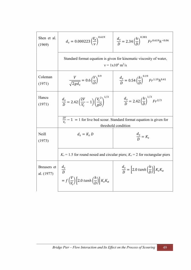
Bridge Pier – Flow Interaction and Its Effect on the Process of Scouring 49
Shen et al.
(1969)
Standard format equation is given for kinematic viscosity of water,
ν = 1x10⁶ m2/s
Coleman
(1971)
Hancu
(1971)
1 for live bed scour. Standard format equation is given for
threshold condition
Neill
(1973)
Ks = 1.5 for round nosed and circular piers; Ks = 2 for rectangular piers
Breusers et
al. (1977)

Bridge Pier – Flow Interaction and Its Effect on the Process of Scouring 50
; for
; for 0.5<
; for
Standard equation is given at the threshold condition
Jain and
Fischer
(1980)
Standard format equation is given at
the threshold condition
Jain (1981)
Standard format equation is given at the threshold condition
Chitale
(1988)
Melville
and
Sutherland
(1988)
For an aligned pier, ds max = 2.4 KsKd. Standard format equation is
given at threshold condition

Bridge Pier – Flow Interaction and Its Effect on the Process of Scouring 51
Froehlich
(1988)
Dp = projected width of pier;
Breusers
and
Raudkivi
(1991)
For an aligned pier dmax =
Richardson
and Davis
(1995)
Ansari and
Qadar
(1994)
for
for
for
for
Wilson
(1995)
effective width of pier
2.3.8.1 Laursen and Toch Method Laursen and Toch (1956) developed a series of design curves based on their prototype
model studies. According to the citation made on Melville and Sutherland (1988), the
curves were later presented in the form of a mathematical formula by Neill (1964). The
equation is expressed as:

Bridge Pier – Flow Interaction and Its Effect on the Process of Scouring 52
2.37
2.3.8.2 Melville and Coleman Method Melville and Coleman (2000), presented a modified form of scour depth prediction
equation, initially proposed by Melville (1997), inserting a time factor suggested by
Melville and Chiew (1999). The equation consists of various multiplying factors for the
effects of the various parameters influencing the scour depth. Equation 2.38 represents
this modified equation for the scour depth prediction. This equation is applicable to
predict the equilibrium local scour depth only.
2.38
where,
KhD = depth size factor
KI = Flow intensity factor
Kd = Sediment size factor
Kα = Pier alignment factor
Ksh = Pier shape factor
KG = Channel geometry factor
Kt = Time factor
The above factors are presented in Table 2.4.
Table 2.4 Different correction factors of Equation 2.38 (after Melville and Coleman, 2000)
Flow depth-pier size factor, KhD
2.39a
2.39b

Bridge Pier – Flow Interaction and Its Effect on the Process of Scouring 53
2.39c
Flow intensity factor, KI
2.40a
2.40b
Sediment size factor, Kd
2.41a
2.41b
Pier alignment factor, Kα
2.42
Pier shape factor, Ksh for uniform pier Ksh
Circular 1.0
Round Nosed 1.0
Square Nesed 1.1
Sharp Nosed 0.9
Time factor, Kt as per Equations 2.34, 2.35 and 2.36

Bridge Pier – Flow Interaction and Its Effect on the Process of Scouring 54
Additionally, Melville and Coleman (2000) presented the pile group shape factor for a
pier comprising a row of cylindrical columns in terms of flow angle, diameter of the
column, spacing between two columns. These shape factors are based on the data
provided by Hannah (1978) and is represented by KshKα , as summarised in Table 2.5.
Table 2.5 Shape factor (KshKa) for multiple columns aligned in a row (after Melville and Coleman, 2000)
S.N. L/D KshKα
α < 5° α = 5° to 45° α = 90°
1 2 1.12 1.4 1.2
2 4 1.12 1.2 1.1
3 6 1.07 1.16 1.08
4 8 1.04 1.12 1.02
5 10 1.00 1.00 1.00
In order to predict the maximum scour depth around the group of piles, Ataie-Ashtiani
and Beheshti (2006) have proposed a multiplying factor (KGmn) obtained by using their
own data and others pre-existing scour data. The value of KGmn can be computed from
Equation 2.43 as follows:
2.43
Where, m = number of piles in line with the flow; n = numbers of piles normal to the flow
and G = spacing between two columns measured inner-to-inner face (clear spacing
between two columns).
2.3.8.3 HEC-18 Equation
Another famous equation, proposed by Richardson and Davis (2001) to estimate local
scour depth, is the HEC-18 equation. The equation is also widely known as the Colorado
State University Equation (CSU Equation), which is expressed as:

Bridge Pier – Flow Interaction and Its Effect on the Process of Scouring 55
2.44
where,
K1 = adjustment factor for pier shape
K2 = adjustment factor for angle of attack
K3 = adjustment factor for bed condition
Kw = adjustment factor for wide pier
Fr = Froude number =
In the above equation, the values of K1, K2 and K3 for various conditions are presented
in Tables 2.6, 2.7 and 2.8, respectively as follows:
Table 2.6 Correction factor K1 for pier nose shape (after Richardson and Davis, 2001)
S.N Shape of Pier Nose K1
1 Square nose 1.1
2 Round nose 1.0
3 Circular cylinder 1.0
4 Group of cylinders 1.0
5 Sharp nose 0.9
Table 2.7 Correction factor K2 for angle of attack (after Richardson and Davis, 2001)
S.N Angle L′/D = 4 L′/D = 8 L′/D = 12
1 0 1.0 1.0 1.0
2 15 1.5 2.0 2.5
3 30 2.0 2.75 3.5
4 45 2.3 3.3 4.3
5 90 2.5 3.9 5.0
Where, Angle = skew angle of flow; L′ = length of pier
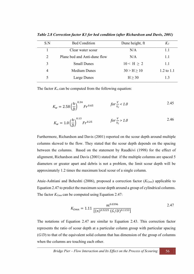
Bridge Pier – Flow Interaction and Its Effect on the Process of Scouring 56
Table 2.8 Correction factor K3 for bed condition (after Richardson and Davis, 2001)
S.N Bed Condition Dune height, ft K3
1 Clear water scour N/A 1.1
2 Plane bed and Anti-dune flow N/A 1.1
3 Small Dunes 10 < H ≥ 2 1.1
4 Medium Dunes 30 > H ≥ 10 1.2 to 1.1
5 Large Dunes H ≥ 30 1.3
The factor Kw can be computed from the following equation:
for < 1.0 2.45
for > 1.0 2.46
Furthermore, Richardson and Davis (2001) reported on the scour depth around multiple
columns skewed to the flow. They stated that the scour depth depends on the spacing
between the columns. Based on the statement by Raudkivi (1998) for the effect of
alignment, Richardson and Davis (2001) stated that if the multiple columns are spaced 5
diameters or greater apart and debris is not a problem, the limit scour depth will be
approximately 1.2 times the maximum local scour of a single column.
Ataie-Ashtiani and Beheshti (2006), proposed a correction factor (KGmn) applicable to
Equation 2.47 to predict the maximum scour depth around a group of cylindrical columns.
The factor KGmn can be computed using Equation 2.47:
2.47
The notations of Equation 2.47 are similar to Equation 2.43. This correction factor
represents the ratio of scour depth at a particular column group with particular spacing
(G/D) to that of the equivalent solid column that has dimension of the group of columns
when the columns are touching each other.

Bridge Pier – Flow Interaction and Its Effect on the Process of Scouring 57
2.3.8.4 Sheppard/Melville Equation
Sheppard et al. (2014) proposed a method to predict the equilibrium scour depth
combining the previous equations suggested by Sheppard and Miller (2006) and Melville
(1997). The equations were slightly modified to form a new equation, referred as the
Sheppard/Melville equation or simply the S/M equation. The results from the study show
that the S/M equation exhibits the best performance among tested equations and is
recommended to be applied in the prediction of equilibrium scour depths. The equations
are:
for 0.4 ≤ ≤1.0 2.48
for 1 ≤ ≤ 2.49
for > 2.50
2.51
2.52
2.53
where Vlp is the live bed peak velocity which can be computed as the larger of the values
from following equations:
2.54
2.55

Bridge Pier – Flow Interaction and Its Effect on the Process of Scouring 58
The sediment critical velocity, Vc, used in the above mentioned equations can be
computed using Shield’s diagram as discussed in Section 2.3.1.1.
2.4 Open Channel Flow and Flow around Bridge Piers
It is essential to understand the hydraulics of open channel flow and sediment transport
for the study of flow and scour around the hydraulic structures like bridge piers. The
nature of flow in an open channel is highly dependent on the types of boundary. Flow
over a moveable boundary behaves differently from the rigid boundary flow. When the
bed materials start to move, there is an interaction between flow and the boundary,
resulting in a complex nature of flow. However, to understand the flow in moveable
boundary channels, the basic concept of flow over rigid boundaries should be reviewed
and the hydraulics of moveable boundary channels can be introduced.
2.4.1 Hydraulics of Open Channel Flow
An open channel flow is simply a free surface fluid flow, which describe the fluid motion
in open channel for example Chaudhry (2007) and Chanson (2004). The fundamental
types of open channel flow are based on the change in velocity of flow with respect to
time and space which are described as follows:
Considering time as a criterion, open channel flow can be classified as:
1. Steady flow: The flow is considered as steady if the depth of flow and hence the
velocity of flow at a point does not change over time. Mathematically it can be
expressed as ∂v/∂t = 0, where ∂v is the variation of the flow velocity at a given
point over the elapsed time ∂t.
2. Unsteady flow: In this type of flow, the depth of flow and the velocity of the flow
at a point change with time i.e. ∂v/∂t ≠ 0.
On the other hand, open channel flow can be classified according to the space criterion
as follows:
1. Uniform flow: The flow will be considered uniform if the magnitude and
direction of the velocity of flow at a given instant of time is the same at every

Bridge Pier – Flow Interaction and Its Effect on the Process of Scouring 59
section of the channel. To fulfill this condition of flow, the cross section of the
channel should be identical in size, shape and orientation. Mathematically it can
be expressed as ∂v/∂x = 0 and ∂v/∂n = 0, where ∂x represents the distance travelled
by the liquid particles, ∂v is the variation in the velocity while travelling the
distance ∂x and ∂n is the direction normal to the flow direction.
2. Varied flow: If the flow velocity at a time varies with respect to distance, the flow
is known as varied flow or non-uniform flow. Mathematically it is expressed as
∂v/∂x ≠ 0 and ∂v/∂n ≠ 0. Depending upon the rate of variation of velocity with
respect to distance, varied flow in an open channel is classified as gradually varied
flow and rapidly varied flow. The flow is said to be gradually varied flow if the
flow characteristics varies at a slow rate with respect to the distance. However, if
the flow characteristics change significantly over a comparatively short distance,
it is known as rapidly varied flow.
Furthermore, there are other types of open channel flow, which are governed to a large
degree by viscosity, gravity and inertial forces. Considering the effect of viscosity, the
flow may be laminar or turbulent flow; whereas, the flow can be classified as subcritical,
supercritical and critical depending upon the effect of gravity relative to inertia.
1. Laminar and turbulent flows: The magnitude of viscous force relative to the
inertial force determines whether the flow is laminar or turbulent. If the viscous
forces are so strong relative to the inertial forces, then the flow is laminar.
However, in turbulent flow, viscous forces are weak relative to the inertial forces.
The ratio of viscous forces and inertial forces is defined as the Reynolds number
and is given by Equation 2.56.
2.56
where, Re is Reynolds number; V is the mean velocity of flow, l is the
characteristic length and ν is the kinematic viscosity of the fluid.
Bridge Pier – Flow Interaction and Its Effect on the Process of Scouring 60
For laminar flow, the value of Re is small, normally less than 500. However for
turbulent flow the value of Re is large, usually greater than 2000. When the value
of Re falls between 500 and 2000, the flow is called mixed or transitional flow.
2. Subcritical, supercritical and critical flows: When the velocity of flow is equal
to the velocity of the gravity wave having small amplitude, the flow is known as
critical flow. For subcritical flow, the flow velocity is less than that of critical
flow. Whereas, for the supercritical flow, the flow velocity is greater than the
critical velocity. The Froude number, Fr, defines the state of the flow as critical,
subcritical and supercritical which is equal to the ratio of inertial and gravitational
forces. For a rectangular channel, Froude number is defined by Equation 2.57
given as under:
2.57
where, Fr is Froude number, h is flow depth, g is acceleration due to gravity and
V is velocity of flow.
Depending upon the value of Fr, flow is classified as subcritical if Fr is less than
1; critical if Fr is equal to 1; and supercritical if Fr is greater than 1. 2.4.2 Basic Equations for Flow in Open Channels
Three laws of conservation were reported to describe the steady and free surface flows,
which were named as conservation of mass, conservation of momentum and conservation
of energy. Based on these laws, important basic equations governing the open channel
flow have been derived and presented.
2.4.2.1 Continuity Equation
Conservation of mass states that the mass rate of steady flow is the same at all sections
of the channel. For a constant density of fluid throughout the sections, the mass rate can
be interpreted as a volumetric rate, or flow discharge.
In Figure 2.23, consider the flow of an incompressible liquid in a channel with no inflow
or outflow across the channel boundaries; the continuity equation is given as:

Bridge Pier – Flow Interaction and Its Effect on the Process of Scouring 61
2.58
Equation 2.58 is valid for non-uniform mean velocities of V1 and V2 at sections 1 and 2
respectively.
Figure 2.23 Notations for continuity equations; (after Chaudhry, 2007)
2.4.2.2 Momentum Equation
The principle of conservation of momentum is defined as the time rate of change of
momentum in the body of water flowing in a channel is equal to the resultant of all the
external forces acting on the body. This conservation of momentum is based on Newton’s
second law of motion.
As shown in Figure 2.24, consider that V1 and P1 are the velocity of flow and the pressure
force in Section 1 respectively and V2 and P2 are the velocity of flow and Pressure force
acting at Section 2 respectively, then according to the principle of conservation of
momentum, total resultant force acting on a body of water is given by Equation 2.59.
Figure 2.24 Notations for momentum equations and application; (after Chaudhry, 2007)

Bridge Pier – Flow Interaction and Its Effect on the Process of Scouring 62
2.59
where, FT is the total external forces acting on a body of water, β is momentum
coefficient.
If W is the weight of water between Section 1 and 2, θ is the slope of the channel and Fe
is the external force due to shear between the liquid and the channel sides, then the
resultant force acting on a body of water along direction of flow is given by Equation
2.60
2.60
2.61
Now from Equations 2.59 and 2.61,
2.62
Equation 2.62 is the momentum equation for steady flow.
2.4.2.3 Energy Equation
The principle of conservation of energy states that total energy of the closed system
cannot change, though it can be conserved over time. According to this principle, in
Figure 2.25, the total energy head at Section 1 should be equal to the total energy head at
Section 2 plus the head loss between these two sections. Mathematically it is expressed
in Equation 2.63 as presented in Simons and Senturk (1992).

Bridge Pier – Flow Interaction and Its Effect on the Process of Scouring 63
Figure 2.25 Notations for energy equations
2.63
where z is the elevation of the channel bed, h is the depth of flow, α is the energy
coefficient and hf is the loss of energy. The subscripts 1 and 2 represent the flow
conditions at Sections 1 and 2. All the notations are clearly shown in Figure 2.25. For a
small channel slope, Equation 2.63 can be reduced to:
2.64
2.4.3 Boundary Layer in Open Channel Flow
In the field of fluid mechanics and hydraulic engineering, a boundary layer is defined as
the layer of fluid close to the bounding surface, where the flow experiences a significant
effect of viscosity. Figure 2.26 schematically shows a boundary layer development in an
open channel flow with an ideal entrance condition. The development of a boundary layer
in open channel is clearly presented by Simons and Senturk (1992). As shown in Figure
2.26, it can be considered that flow at the upstream of point A is uniform where the
velocity of flow, V, is constant. As the flow enters the channel, the friction between flow
and the bottom of the channel alters the flow pattern with the development of laminar

Bridge Pier – Flow Interaction and Its Effect on the Process of Scouring 64
flow between the boundary and the line AB. The velocity distribution above the laminar
boundary line AB remains uniform downstream of point A. Due to the surface roughness
of the boundary, small eddies appear at the top of the rough layer. However they are
suppressed in laminar flow. As the flow velocity increases in the downstream direction,
the size of eddies increases; and at the downstream of point B they reach to the top of the
laminar flow region. After point B, eddies are stronger so that there is a generation of
turbulence along line BC. The thickness of the laminar layer decreases as the turbulence
increases. Now the resulting velocity distribution is parabolic in the laminar flow region
and logarithmic in the turbulent flow region.
Figure 2.26 Development of boundary layer in open channel (Simons, 1992)
The thickness of the boundary sub layer, δ, is defined as the distance between the
boundary and the point at which the viscous flow velocity is 99% of the free-stream
velocity. According to Schlichting and Gersten (1999), the laminar boundary layer
thickness for a flat plate of length of l can be estimated by considering the equilibrium
condition of inertial forces and frictional forces and is represented by Equation 2.65.
2.65

Bridge Pier – Flow Interaction and Its Effect on the Process of Scouring 65
where is the Reynolds number with respect to the plate length and x is the distance
from the leading edge along the flat plate.
Similarly the turbulence boundary layer is the turbulent flow region, the thickness of
which is called the thickness of turbulence boundary layer. In Figure 2.26, it is
represented by δo. The flow downstream side of the section CD is the zone of fully
developed turbulent flow. Simons and Senturk (1992) further presented three different
regimes of roughness with different values of δ. The first roughness regime is a
hydraulically smooth regime for which , where = the
roughness of the sand, which is also known as Nikuradse sand roughness and is equal to
the mean diameter of the sands. In this regime, the size of the roughness of elements is
small and all the protrusions are contained within the laminar sub layer. The second
roughness regime is the transition regime for which . In
this regime, the roughness partly extends through the laminar sub layer, causing
additional resistance to flow. The last regime is the hydraulically rough regime for
which . In this regime all protrusions extend through the laminar sub
layer, causing the largest part of resistance to flow. According to Schlichting and Gersten
(1999), the boundary layer on a plate remains laminar close to the leading edge and
becomes turbulent at the downstream side. At the transition from laminar to turbulent
flow, there is significant increase in the boundary layer thickness.
2.4.4 Turbulence in Open Channel Flow
The flows in most of the hydraulic structures such as spillways, weirs, irrigation channel
and water supply systems are turbulent. In turbulent flow, the velocity and pressure vary
with time and space. If u, v and w are the instantaneous velocity components at a point;
and are the mean components of velocities; and u′, v′ and w′ are the fluctuating
components of velocity in the stream-wise, transverse and vertical directions respectively,
then the relating equations can be written as:
2.66
2.67
Bridge Pier – Flow Interaction and Its Effect on the Process of Scouring 66
2.68
The root mean square value of u′, v′ and w′ are the turbulence intensity components. The
turbulence intensity is given by:
2.69
Based on the velocity fluctuation components, the turbulence kinetic energy (TKE) of the
flow can be determined. In fluid dynamics, the turbulence kinetic energy is defined as the
mean kinetic energy per unit mass associated with eddies in turbulent flow. Generally,
the TKE can be determined by taking the mean of the turbulence normal stresses and is
expressed as in Equation 2.70.
2.70
Furthermore the fluctuating parts of the velocity can be used to quantify the Reynolds
stress, which is the total stress tensor in a fluid. The components of Reynolds stress tensor
are defined by:
2.71
2.72
2.73
2.4.5 Flow around Bridge Piers
Extensive investigations have been carried out on local scour around bridge piers installed
in cohesion-less sediments. Based on these investigations large numbers of studies have
been published. Most of the investigations until this date are focused on the bridge piers
with a single column. Very limited studies have been made on the piers with multiple in-

Bridge Pier – Flow Interaction and Its Effect on the Process of Scouring 67
line columns. In the previous publications, it was reported that the flow structure around
the bridge piers is very complicated and hence the accurate prediction of scour depth is a
very challenging task. In the following sections, review of flow structures around the
bridge piers and scour around the bridge piers are presented.
Scouring around the bridge piers is considered one of the main reasons for bridge failure.
Hence, it creates a great threat to the stability of a bridge structure and the load carrying
capacity of the bridge. It can be noticed from the previous investigations on scour around
bridge piers, most of the studies were based on behaviour of a single pier. However, in
actual practice, the bridge piers in rivers are generally installed in the form of two or more
sequential columns aligned in the flow direction. When the flow of the river is obstructed
by a hydraulic structure such as bridge piers, there is the formation of a complex three
dimensional flow structure. Because of the complex characteristics of the three
dimensional flow structures around the piers, it is difficult to predict the maximum scour
depth. Therefore, to estimate scour depth precisely, it is necessary to understand the
mechanism of flow structure around the bridge piers. Many investigators, such as
Melville (1975); Melville and Raudkivi (1977a); Baker (1979); Dargahi (1989); Salim
and Jones (1996); Ahmed and Rajaratanam (1997); Richardson and Panchang (1998);
Meneghini et al. (2001); Muzzammil and Gangadhariah (2003); Raben et al. (2010);
Shrestha et al. (2012); Kumar and Kothyari (2012a); Shrestha et al. (2013), Ataie-
Ashtiani and Aslani-Kordkandi (2013) among others have conducted research on flow
structures around bridge piers.
As described in Section 2.3.3, the flow-field around a bridge pier is characterized by the
vortex system which consists of a horseshoe vortex system that wraps around the base of
the pier, the bow wave near the free surface at the upstream face of the pier, and the wake
vortex system behind the pier that extends over the depth of flow. According to Dey and
Bose (1994), these flow features have very complex flow structure, which makes it more
complicated to understand the flow field around bridge piers.
2.4.5.1 Horseshoe Vortex System
Two types of horseshoe vortex system namely: a laminar horseshoe vortex system and a
turbulent horseshoe vortex system, were reported in the literature by several investigators,

Bridge Pier – Flow Interaction and Its Effect on the Process of Scouring 68
such as Baker (1979); Baker (1980); Lin et al. (2002a); Muzzammil and Gangadhariah
(2003); Kirkil (2008); and Huang et al. (2014). Baker (1979) reported that the horseshoe
vortex system will be formed at the junction of obstacles like bridge piers in river flow.
This horseshoe vortex system will produce high bed shear stresses on the river bed which
will cause the erosion of bed materials and hence there will be formation of scour hole
around the base of the bridge piers.
Baker (1979) conducted extensive experiments in a smoke tunnel using flow
visualization methods and described the horseshoe vortex system at upstream of the
cylinders mounted on a wall where the laminar boundary layer is growing. During the
experiments both the steady and oscillating vortex system were observed. It was
concluded from the experiments that in steady horseshoe vortex systems, 2, 4 or 6
numbers of vortices were formed. Increase in Reynolds number results in the increase in
the number of vortices. He further reported that the horseshoe vortex system exhibit a
regular oscillatory motion which was found to be complex. As the Reynolds number
increased, steady horseshoe vortex systems began to oscillate intermittently and
randomly. For a higher value of Reynolds number, the oscillations became irregular and
the horseshoe vortex system became turbulent. Lin et al. (2002a) studied the horseshoe
vortex system near the junction of a vertical plate normal to the flow. Depending on the
Reynolds number and height to width ratio (H/W) of the vertical plate, the vortex system
was classified as steady vortex system, periodic oscillation vortex system with small
displacement, periodic break way vortex system, and turbulent like vortex system. It was
reported that this classification was independent of the height to boundary layer thickness
(H/δ) in the range of H/W = 0.5 - 4.0.
On the other hand Baker (1980) conducted an experimental investigation on the
horseshoe vortex system inside a turbulent boundary layer at upstream of a circular
cylinder. The flow topology on the bed and in the plane of symmetry was studied in that
investigation. It was observed from the experiments that the predominant structure of the
turbulent horseshoe vortex system contained two primary vortices. One was observed
attached to the bed and the other smaller intermittent vortex was observed near the
cylinder base. Dargahi (1989) investigated the turbulent horseshoe vortex system for a
wide range of Reynolds number (8400 to 46000) and observed that the vortices were shed

Bridge Pier – Flow Interaction and Its Effect on the Process of Scouring 69
from the separation region similar to the laminar horseshoe vortex case. It was reported
that in most of the cases, the horseshoe vortex system contained three primary vortices
rotating in the same direction and two bed-attached vortices rotating in the opposite
direction.
2.4.5.2 Vortex Shedding
Vortex shedding is a phenomenon in which the flow oscillates behind the hydraulic
structure. When the flow of fluid is disrupted by an obstruction, vortices are created at
the back of the obstruction and detach periodically. Due to this detachment, unsteady
flow is created. According to Sumer and Fredsøe (1997), vortex shedding phenomenon
is the most important feature of the flow regimes around the bridge piers with Reynolds
number (Re) > 40. The flow regimes changed as the Re increased. Figure 2.27 gives the
definition sketch of wake region and boundary layer region. As shown in the Figure 2.27,
the wake region extends over a distance at the downstream side of the pier which is
comparable to the diameter of the pier, D, while the boundary layer extends over a very
small thickness, δ. The dependency of the laminar boundary layer with the Re is given by
Schlichting and Gersten (1999) which is expressed in Equation 2.74. From this equation,
it can be seen that for Re larger than 100, the value of δ/D is less than 1.
2.74
Figure 2.27 Definition sketch of flow regions; (after Sumer and Fredsoe, 1997)

Bridge Pier – Flow Interaction and Its Effect on the Process of Scouring 70
On the other hand Figure 2.28 shows the summarization of changes in flow regimes with
increase in Re. The flow regimes around the cylindrical objects with respect to Re are
studied by several investigators; for example Bloor (1964); Gerrard (1978); Williamson
(1988); Williamson (1989); Sumer and Fredsøe (1997); Batchelor (2000). As reported
by Sumer and Fredsøe (1997), it is clear from Figure 2.28 that for Re < 5, the boundary
layer separation does not occur. When the range of Re is between 5 and 40, a pair of
vortices form at the wake of the cylinder. Increase in the value of Re also increases the
length of vortex formation. Further increase in the value of Re results in an unstable wake.
Eventually other vortices are generated and are shed alternately at either side of the
cylinder. When the range of Re is between 40 and 200, the resulting vortex shedding is
called laminar vortex shedding. Further increasing the range of Re between 200 and 300,
transition to turbulence occurs. For Re > 300, the wake is completely turbulent; however
the boundary layer over the cylinder remains laminar until the value of Re become less
than 3 × 10⁵. This regime is known as subcritical flow regime. With further increase in
Re to 3.5 × 10⁵, the boundary layer becomes turbulent at only one side of the cylinder and
the boundary layer on the other side remains laminar. Such type of flow regime is called
critical flow regime. When the Re is between 3.5 × 10⁵ and 1.5 × 10⁶, this regime is called
supercritical flow regime where turbulent boundary layer separation occurs on both sides
of the cylinder. Further increase in Re value greater than 1.5 × 10⁶ makes the regime fully
turbulent. In this flow regime, the boundary layer is partly laminar and partly turbulent.
This regime is called the upper transition flow regime which exists until Re is less than
4.5 × 10⁶. Finally for the value of Re greater than 4.5 × 10⁶, the regime is called trans
critical flow regime in which the boundary layer on the cylinder surface is virtually
turbulent everywhere.
The study on fluid dynamics of multiple cylinder configurations have been carried by
several researchers, for example Zdravkovich (1977); Zdravkovich (1987); Gu (1996);
Sumner et al. (2000); Lin et al. (2002b) and Sumner (2010). Sumner (2010) reported that
when two cylinders are placed in tandem arrangements, the different flow regimes are
observed. The complex interactions between the shear layers, vortices, wakes and
Karman vortex streets of the flow field are generated due to the configuration of multiple

Bridge Pier – Flow Interaction and Its Effect on the Process of Scouring 71
cylinders. The flow regime in this case basically depends on the spacing between two
cylinders, orientation of the cylinders and the Reynolds number.
The fluid behaviour for two cylinders is theoretically approached in a simplified way by
Zdravkovich (1987). He classified two basic types of interference which are based on the
location of the downstream cylinder with respect to the upstream one. The interference
regions are wake interference and proximity interference as shown in Figure 2.29. The
wake interference exists when one of the cylinders is partially or completely submerged
in the wake of the other i.e. cylinders are placed in tandem or staggered arrangements.
While the proximity interference occurs when cylinders are placed in side by side
arrangements. In the proximity interference, neither of the cylinders is submerged in the
wake of others.

Bridge Pier – Flow Interaction and Its Effect on the Process of Scouring 72
Figure 2.28 Flow regimes around smooth circular cylinder in steady current, (Sumer and Fredsoe, 1997)
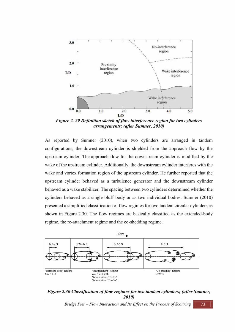
Bridge Pier – Flow Interaction and Its Effect on the Process of Scouring 73
Figure 2. 29 Definition sketch of flow interference region for two cylinders
arrangements; (after Sumner, 2010)
As reported by Sumner (2010), when two cylinders are arranged in tandem
configurations, the downstream cylinder is shielded from the approach flow by the
upstream cylinder. The approach flow for the downstream cylinder is modified by the
wake of the upstream cylinder. Additionally, the downstream cylinder interferes with the
wake and vortex formation region of the upstream cylinder. He further reported that the
upstream cylinder behaved as a turbulence generator and the downstream cylinder
behaved as a wake stabilizer. The spacing between two cylinders determined whether the
cylinders behaved as a single bluff body or as two individual bodies. Sumner (2010)
presented a simplified classification of flow regimes for two tandem circular cylinders as
shown in Figure 2.30. The flow regimes are basically classified as the extended-body
regime, the re-attachment regime and the co-shedding regime.
Figure 2.30 Classification of flow regimes for two tandem cylinders; (after Sumner, 2010)

Bridge Pier – Flow Interaction and Its Effect on the Process of Scouring 74
For the condition of extended body regime, Zdravkovich (1987) suggested the ranges of
L/D ratios as 1 < L/D < 1.2-1.8, while Zhou and Yiu (2006) suggested as 1 < L/D < 2. For
these ranges of L/D values, the two cylinders act as a single bluff body in which the free
shear layers separated from upstream cylinders wrap around the downstream cylinder,
without any re-attachment onto its surface. It was reported by Sumner (2010) that in this
regime, the downstream cylinder is positioned inside the vortex formation region of the
upstream cylinder. The shear layers detached from the upstream cylinder elongate
significantly larger than that of the single cylinder case. The vortex behind the
downstream cylinder occurs closer to the cylinder when compared to the single cylinder.
The re-attachment regime occurs in the range of 1.2-1.8 < L/D < 3.4-3.8 or 2 < L/D < 5
as reported by Zdravkovich (1987) or Zhou and Yiu (2006), respectively, depending on
the value of the Reynolds number. In this regime, the two cylinders are sufficiently far
apart that the shear layer detached from the upstream cylinder re-attach on the upstream
side of the downstream cylinder. However the vortex street is formed only behind the
downstream cylinder. According to Lin et al. (2002b) the re-attachment regime is
principally characterized by the re-attachment of the shear layer from the upstream
cylinder, and formation and shedding of eddies in the gap between the two cylinders.
Eddies in the gap substantially and intermittently vary in terms of their strength,
asymmetry, and general behaviour.
The co-shedding regime occurs in the range of L/D > 3.4 - 3.8 as reported by Zdravkovich
(1987) or L/D > 5 as reported by Zhou and Yiu (2006), respectively, in which the two
cylinders are placed in such a way that the vortex shedding occur from both upstream and
downstream cylinders. Zdravkovich (1987) reported that in this regime, the vortex
shedding behind the downstream cylinder is called binary vortices. Furthermore, Sumner
(2010) reported that in the co-shedding regime, both the cylinders undergo vortex
shedding of the same frequency; and the vortex shedding behind the downstream cylinder
is disturbed by the vortices generated by upstream cylinder. The resulting vortices behind
the downstream cylinder are larger but weaker than those of the extended-body and re-
attachment regimes. Hence the vortices shaded from the downstream cylinder dissipate
quickly.

Bridge Pier – Flow Interaction and Its Effect on the Process of Scouring 75
2.4.5.3 Vortex Strength and Size
As the horseshoe vortex system at upstream of the bridge pier is the most significant
parameter in the scour process, it is very important to analyze its strength and size. It was
reported in most of the previous research that the horseshoe vortex system depends on
the diameter of the pier and the approach flow velocity. As reported by Lee (2006), the
vortex strength is defined as circulation around a vortex core, which can be
mathematically expressed as in Equation 2.75:
2.75
where,
R = radius of the vortex
Vθ = tangential vortex velocity = ω0R
ω0 = angular velocity of revolution
It was experimentally hypothesized by Qadar (1981) that the maximum value of scour
depth should necessarily be a function of the initial vortex strength. The initial vortex
strength, , can be defined by Equations 2.76 - 2.79.
2.76
for, D 2.77
for, D 2.78
2.79
Kothyari et al. (1992) suggested a mathematical expression for the diameter of the
primary vortex using the experimental data from other investigators, for example. Baker
(1979); Qadar (1981); Muzzamil et al. (1989); and from his own experiments, which is
Bridge Pier – Flow Interaction and Its Effect on the Process of Scouring 76
given in Equation 2.80. Furthermore it was reported that the size of the horseshoe vortex
is also affected by the bridge opening ratio, (W-D)/W, where W is the width of the flume
or span-wise spacing between two piers.
2.80
where D is the diameter of the bridge pier, h is the depth of flow and R is the radius of
the vortex.
According to Muzzammil and Gangadhariah (2003), for higher values of pier Reynolds
number, the size of the vortex is only dependent on the diameter of the pier. They
suggested that the size and tangential velocity of the vortex are given in Equations 2.81
and 2.82:
For, Re 2.81
2.82
where f is the frequency of rotation of the vortex. Substituting the value of Vθ from
Equation 2.82 to Equation 2.75 gives vortex strength as in Equation 2.83.
2.83
2.4.5.4 Frequency of Vortex Shedding
Referring to previous studies it can be found that wake vortices play an important role in
the scouring phenomenon in the wake region of the bridge piers. Lee (2006) reported that
the wake vortices contribute in the movement of the sediment particles through the
process of suspending, sliding, rolling and jumping. Hence, studying the flow structure
in the wake region is very important to predict the scour depth around bridge piers. As
the detached boundary layers from two sides of the piers are directed towards the

Bridge Pier – Flow Interaction and Its Effect on the Process of Scouring 77
centreline and curl back forming vortices which extend over a distance at the downstream
side of the pier which is comparable to the diameter of the pier, D. The vortex is initially
formed at one side of the pier, moving to the downstream side becoming larger in size
and strength and is finally shed at a constant frequency. The shedding is followed by
formation of a vortex on the other side of the piers. This phenomenon of altering of
vortices at constant space is called vortex shedding. Figure 2.31 shows the schematics of
the of vortex shedding behind the bridge piers.
Figure 2.31 Schematics of vortex shedding a) Prior to shedding of Vortex A, Vortex B is being drawn across the wake, b) Prior to shedding of Vortex B, Vortex C is being
drawn across the wake (Sumer and Fredsoe, 1997)
The vortex shedding frequency is directly proportional to the flow velocity and inversely
proportional to the characteristic length scale (the diameter of the pier). However, it is
independent of fluid properties such as density, viscosity. The vortex shedding frequency
is related to the Strouhal number, which is given by the following equation:
2.84
where, St = the Strouhal number; f = the vortex shedding frequency; D = the diameter
of the pier; and V = the velocity of flow.
Sumer and Fredsøe (1997) stated that the Strouhal number is defined as the normalized
vortex shedding frequency. They presented the variation of Strouhal number with
Reynolds number using the different experimental data from previous researches as
shown in Figure 2.32. It is clear from the figure that the St is 0.1 at Re = 40 at which the
vortex shedding first appears. Then it increases gradually as Re increases and attains a
value of about 0.2 when the value of Re is about 300. Further increase in the value of Re

Bridge Pier – Flow Interaction and Its Effect on the Process of Scouring 78
about 3 x 10⁵, St remains more or less constant at the value of approximately 0.2. After
this, St experiences a sudden jump at Re = 3 - 3.5 × 10⁵, where St increases from 0.2 to a
value of about 0.45. This high value of St is maintained over the range of Re = 3 × 10⁵ to
2 × 10⁶; subsequently it decreases slightly with increasing the value of Re.
Figure 2.32 Strouhal number as a function of Reynolds number; (Sumer and Fredsoe, 1997)
2.5 Summary and Identification of the Gap in Literature
In this chapter, a detailed review of the available literature related to the scour problem
around bridge piers has been presented. Different topics such as the general definition
and classification of the scour at the bridge crossings, the mechanism of local scour and
the effect of different factors that influence the local scour depth, methods of estimating
the scour depth, flow regimes around the bridge piers have been described in detail.
Basically, scour is the consequence of the interaction between flow and hydraulic
structures such as bridge piers placed in flowing water in which the sediment material is
removed and eroded from the bed and the banks of the streams and also from the vicinity
of the hydraulic structures. In Section 2.2 general definitions of scour as presented in
various previously published studies have been outlined. Furthermore, the types of scour

Bridge Pier – Flow Interaction and Its Effect on the Process of Scouring 79
are presented in this section according to which scour can occur at a bridge crossing; these
types are broadly classified as general scour, contraction scour and local scour.
Section 2.3 describes the local scour, classification of local scour and the mechanism of
local scour. The classification of local scour is primarily based on the amount of material
supplied into the scour area and the capacity of flow to transport the sediment. According
to this, it is described that two types of local scour exist namely: clear water scour and
live bed scour. The clear water scour and live bed scour are determined by the critical
mean velocity of flow, which can be calculated using Equation 2.12. Additionally, the
effect of various parameters (for example the velocity of flow, the depth of flow, the size
and shape of piers, the size of bed materials) on the local scour depth around bridge piers
has been presented in this section. The general concept of sediment transport phenomenon
and beginning of sediment motion has been briefly described, which gives a better
understanding of scour around hydraulic structures. In addition, various equations for
predicting the scour depth around bridge piers, developed in the past studies have been
presented as in Table 2.3. All of these equations were developed for a bridge pier with a
single column. Only a few studies have been carried out on the scour around the bridge
piers with a group of columns.
The basic mechanism of the local scour around the bridge piers has been identified as a
system of vortices developed around the bridge piers. Section 2.4 has been furnished with
the basic concept of open channel for flow that includes types of open channel flow, basic
equations of open channel flow and various turbulence equations. Furthermore, horseshoe
vortex and wake vortex have been described as the primary vortex system that causes the
scour around bridge piers. Hence, the horseshoe vortex system, vortex shedding, vortex
strength and vortex shedding frequency have been presented in section 2.4. Two types of
horseshoe vortex system: laminar horseshoe vortex system and turbulent horseshoe
vortex system have been reported which depend on the values of the Reynolds number.
Moreover, the vortex shedding phenomenon has been identified as an important feature
of flow regimes around the bridge piers. Different types of flow regimes that depend on
the Reynolds number have been presented in Section 2.4. For the case of two in-line
circular cylinders, it has been reported that the flow regimes depend on the spacing
between the two cylinders, orientation of the cylinders and the Reynolds number. The

Bridge Pier – Flow Interaction and Its Effect on the Process of Scouring 80
flow regimes for two in-line circular cylinders have also been categorised as the extended
body regime, the re-attachment regime and the co-shedding regime.
According to the critical review conducted on previous investigations, it is found that
extensive studies have been carried out on scour and flow structure around bridge piers
consisting of a single column and numerous equations have been developed to predict the
equilibrium scour depth. Only a few studies have been conducted for the bridge pier
consisting of a group of piers in a matrix form and are limited to equilibrium scour depth
around the piers. However, in a real situation the majority of bridge structures are
supported by bridge piers comprising two or more in-line columns. By and large, the
scour depth and flow structure behaviour of two in-line columns have not been well
investigated in the past. Hence, the present study mainly focuses on the experimental
investigation on flow structures and scour depth at bridge piers comprising twin circular
columns aligned in the flow direction; and then the effects of spacing between the
columns on flow structures and scour depth are evaluated.

Bridge Pier – Flow Interaction and Its Effect on the Process of Scouring 81
CHAPTER 3
EXPERIMENTAL SETUP AND METHODOLOGY
3.1 Introduction
3.2 Experimental Setup and Design
3.3 Velocity Measurement
3.4 Experimental Procedure and Data Acquisition
3.5 Summary

Bridge Pier – Flow Interaction and Its Effect on the Process of Scouring 82
3. EXPERIMENTAL SETUP AND METHODOLOGY
3.1 Introduction
In this chapter, the experimental arrangements, design of hydraulic models, equipment
used during experiments, data acquisition methods and variables measured in the study
are described. Three sets of laboratory experiments that include flow structure using an
acoustic Doppler velocimeter (ADV), local scour around the bridge piers and flow
structure using particle image velocimetry (PIV) are carried out in this study. All of the
experiments are conducted in the Hydraulics Laboratory at the University of Technology,
Sydney (UTS), Australia.
3.2 Experimental Setup and Design
3.2.1 Flume and its Components
Two different flumes were used to conduct the experimental tests. In this dissertation, the
flumes are denoted by Flume 1 and Flume 2. Both flumes are recirculating flumes and
available in the hydraulics laboratory at UTS. Flume 1 is 19 m long, 0.61 m wide and
0.61 m deep. At the working section of the flume, there is a section in the form of a recess,
which is 5.00 m long and 0.15 m deep, located at 9.0 m downstream from the flume inlet
section. This recess has been filled by sand; thus called the sand recess. Plexiglass
sidewall has been provided along one side of the working section to facilitate visual
observations. A settling chamber has been provided upstream to the inlet section of the
flume. There is also an overhead tank at the upstream side of the flume, into which the
water is pumped from the main reservoir tank. The main function of this overhead tank
is to provide a continuous flow of water at constant rate to the flume. Water from this
overhead tank is supplied to the settling chamber of the flume. A regulating gate has been
provided at the outlet section of the flume, which is used to control the depth of flow in
the flume and hence to control the velocity of flow. The used water from the flume is then
discharged to the outlet tank, which is again sent to the main reservoir. The schematic
diagram of Flume 1 is shown in Figure 3.1. This flume has been used for the study of
local scour around bridge piers and flow structure interactions using an acoustic Doppler
velocimeter (ADV).
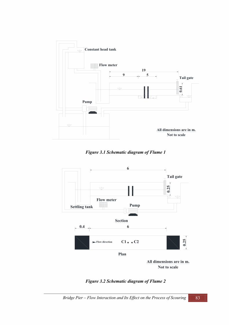
Bridge Pier – Flow Interaction and Its Effect on the Process of Scouring 83
Figure 3.1 Schematic diagram of Flume 1
Figure 3.2 Schematic diagram of Flume 2
199 5
0.61
Flow meter
Pump
Constant head tank
Tail gate
All dimensions are in m.Not to scale
60.
25
Tail gate
C2C1
Section
Plan
Flow direction
All dimensions are in m.Not to scale
PumpFlow meter
Settling tank
0.25
0.4 6

Bridge Pier – Flow Interaction and Its Effect on the Process of Scouring 84
Another flume with a smaller size (Flume 2) with nominal dimensions of 6 m long, 0.25
m wide and 0.25 m deep as shown in Figure 3.2 has been used for the study of flow
structure around the bridge piers under fixed bed condition using particle image
velocimetry (PIV). It is made of a plexiglass sidewall so that the experiments can easily
be monitored all the time. There is a provision of a settling tank at the inlet section, which
supplies water in the flume. There is another tank installed at the outlet section from
where the used water is pumped to the settling tank. This flume has also been equipped
with a flow meter, a regulating gate and a pump.
3.2.2 Electromagnetic Flow Meter
Siemens, MAG 5000 electromagnetic flow meter has been used to measure the flow rate
of water in the flume. The measuring accuracy of the instrument used has been ±0.4% of
the flow rate. This instrument has been placed between the inlet section of the flume and
the outlet of the constant head tank. Figure 3.3 shows a photograph of this
electromagnetic flow meter. As the water flows through this instrument, the amount of
flow is displayed on the digital screen, provided at the top of the instrument.
Figure 3.3 Electromagnetic flow meter (courtesy of Siemens)
3.2.3 Vernier Point Gauge
A vernier point gauge with least count of 0.05 mm has been used to measure the bed
profile. This vernier point gauge has been mounted in such a way that it can move in all
three directions (longitudinal, transverse and vertical directions). Figure 3.4 shows a
photograph of the vernier point gauge used.

Bridge Pier – Flow Interaction and Its Effect on the Process of Scouring 85
Figure 3.4 Vernier point gauge to measure the scour depth
3.2.4 Model Columns of Bridge Piers
Experiments were carried out with a single column and two in-line circular columns.
When two columns were used, they were arranged in such a way that the flow direction
was parallel to the pier alignment i.e. the angle of flow attack was zero. The columns
were installed at the centreline of the flume at the same longitudinal section. Figure 3.5
shows a schematic illustration of the two in-line circular column model.
Figure 3.5 Model columns showing the spacing between them
L
Column 1 Column 2
Flow direction
DD

Bridge Pier – Flow Interaction and Its Effect on the Process of Scouring 86
The column diameter was carefully chosen so that there was no contraction effect on the
depth of scour. According to Melville and Coleman (2000), in-order to avoid the
contraction effect, the flume width should be at least 10 times the column diameter. In
this study, columns with diameters of 55 mm were taken for the tests in Flume 1, and for
the Flume 2, 16 mm diameter columns were adopted. The flume width to the column
diameter ratio (W/D) were 11.27 for Flume 1 and 15.62 for Flume 2, which satisfy the
boundary condition recommended by Melville and Coleman (2000).
3.2.5 Bed Materials
In the case of Flume 1, 150 mm thick sand was placed in the recess at the test section of
the flume. To find the properties and types of sand used for this study, the soil-grading
test (sieve analysis) was carried out in the soils laboratory at UTS. The specification of
the sand used is given in Table 3.1
Table 3.1 Specification of bed material
Parameter Value
Mean particle size, d50 0.85 mm
Specific gravity, ss 2.60
Geometric standard deviation, σg 1.33
Coefficient of uniformity, Cu = d60/d10 1.77
Coefficient of curvature, Cc = (d30)2/(d10 ×d60) 1.10
where, d60 = grain size at 60% passing, d30 = grain size at 30% passing and d10 = grain
size at 10% passing.
The plot of the grain size distribution (sieve analysis) test is shown in Figure 3.6. The
geometric standard deviation of sand is 1.33, the coefficient of uniformity is 1.77 and the
coefficient of curvature is 1.08. According to Melville and Coleman (2000), for uniform
sand, σg should be between 1.3 and 1.5. Additionally, Ameson et al. (2012) reported that
the sand will be considered as uniformly graded when Cu < 6 and 1< Cc <3, where Cu and
Cc are coefficient of uniformity and coefficient of curvature, respectively. The selected
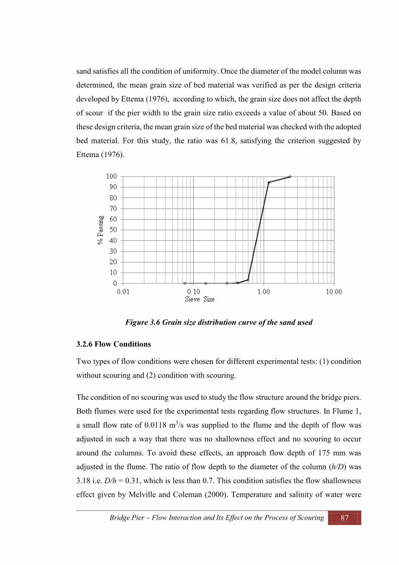
Bridge Pier – Flow Interaction and Its Effect on the Process of Scouring 87
sand satisfies all the condition of uniformity. Once the diameter of the model column was
determined, the mean grain size of bed material was verified as per the design criteria
developed by Ettema (1976), according to which, the grain size does not affect the depth
of scour if the pier width to the grain size ratio exceeds a value of about 50. Based on
these design criteria, the mean grain size of the bed material was checked with the adopted
bed material. For this study, the ratio was 61.8, satisfying the criterion suggested by
Ettema (1976).
Figure 3.6 Grain size distribution curve of the sand used
3.2.6 Flow Conditions
Two types of flow conditions were chosen for different experimental tests: (1) condition
without scouring and (2) condition with scouring.
The condition of no scouring was used to study the flow structure around the bridge piers.
Both flumes were used for the experimental tests regarding flow structures. In Flume 1,
a small flow rate of 0.0118 m3/s was supplied to the flume and the depth of flow was
adjusted in such a way that there was no shallowness effect and no scouring to occur
around the columns. To avoid these effects, an approach flow depth of 175 mm was
adjusted in the flume. The ratio of flow depth to the diameter of the column (h/D) was
3.18 i.e. D/h = 0.31, which is less than 0.7. This condition satisfies the flow shallowness
effect given by Melville and Coleman (2000). Temperature and salinity of water were

Bridge Pier – Flow Interaction and Its Effect on the Process of Scouring 88
also measured prior to the starting of the experiments and found to be 20˚C and 0,
respectively. For each of the flow conditions described above, seven different sets of
columns arrangements (different spacing between the piers) were established and the data
were captured in three different layers for each setup. For Flume 2 a flow rate of 0.003
m3/s and an approach flow depth of 130 mm were established so that there was no
sediment movement around the columns. In this flow condition, the ratio of D/h was
calculated as 0.12, satisfying the condition of flow shallowness as described earlier.
Table 3.2 Flow conditions for experimental tests
Tests Q (m3/s)
h (m)
D (mm)
d50 (mm)
V/Vc Reynolds No. (Re)
Froude No. (Fr)
Remarks
1 0.0118 0.175 55 0.85 0.38 12500 0.068 Flume 1
Fixed bed
2 0.0185 0.115 55 0.85 0.74 22000 0.19 Flume 1
Mobile bed
3 0.0330 0.160 55 0.85 0.91 35500 0.25 Flume 1
Mobile bed
4 0.0315 0.15 55 0.85 0.93 35000 0.22 Flume 1
Mobile bed
5 0.0350 0.16 55 0.85 0.96 37600 0.23 Flume 1
Mobile bed
6 0.003 0.13 16 0.85 0.38 6000 0.041 Flume 2
Fixed bed
Another flow condition was established for the condition of clear water with local scour
around piers. Flow rates, used in this condition, ranged from 0.0185 to 0.033 m3/s and
depth of flow was adjusted in the range of 115 to 160 mm, satisfying the condition of
flow shallowness so that the pier would be considered as a narrow pier. During the
experiments in these conditions, water temperatures were recorded. The temperature

Bridge Pier – Flow Interaction and Its Effect on the Process of Scouring 89
range was between 13˚C and 20˚C. However, according to the experiments conducted by
Melville and Chiew (1999), it was reported that there is no discernible difference in the
scour depth development, or equilibrium scour depth due to temperature variation.
In this study, six sets of tests were carried out as shown in Table 3.2. For each test there
was different subset of tests including a single column, and twin in-line circular columns
with different spacing between them (L/D = 0 to 12). Test 1 and Test 6 were designed to
study the flow structure around the bridge piers. Tests 2 to 5 were designed to study the
scour around bridge piers comprising a single column and twin columns as well as the
influence of pier spacing on scour depth. The incipient motion condition of the sediment
particle was determined according to the procedure given in Section 2.3.1.1.
3.3 Velocity Measurement
During the experiments on flow structures, three dimensional velocity components were
the primary data to be measured. In this study, velocity components were measured using
an Acoustic Doppler Velocimetry and a Particle Image Velocimetry measurement
technique, which are separately described as follows:
3.3.1 Acoustic Doppler Velocimetry (ADV)
An Acoustic Doppler Velocimeter was used to measure the instantaneous three
dimensional velocity components during the experiments on the flow structure in Flume
1. An ADV is a single point current meter that measures the three dimensional velocity
components in high and low flow conditions. An ADV uses an acoustic Doppler
technology to measure three-dimensional velocity in a small sampling volume located a
distance away from the probe head. As per the detail information on SonTek (2001), the
SonTek / YSI 16-MHz MicroADV was used as a current meter, which is optimal for
using in the laboratory. The velocity range is programmable from ± 1 mm/s to ± 2.50 m/s.
Data can be acquired at sampling rates up to 50 Hz. The ADV consists of three basic
elements: the probe, the signal-conditioning module, and the processor. The probe is
attached to the conditioning module, which contains low noise receiver electronics
enclosed in a submersible housing. The ADV conditioning module and probe are
connected to the processing module using a custom shielded cable. The ADV field
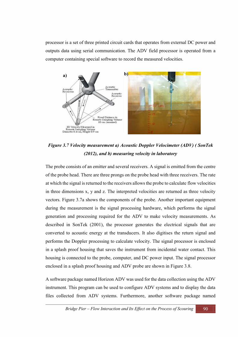
Bridge Pier – Flow Interaction and Its Effect on the Process of Scouring 90
processor is a set of three printed circuit cards that operates from external DC power and
outputs data using serial communication. The ADV field processor is operated from a
computer containing special software to record the measured velocities.
Figure 3.7 Velocity measurement a) Acoustic Doppler Velocimeter (ADV) ( SonTek
(2012), and b) measuring velocity in laboratory
The probe consists of an emitter and several receivers. A signal is emitted from the centre
of the probe head. There are three prongs on the probe head with three receivers. The rate
at which the signal is returned to the receivers allows the probe to calculate flow velocities
in three dimensions x, y and z. The interpreted velocities are returned as three velocity
vectors. Figure 3.7a shows the components of the probe. Another important equipment
during the measurement is the signal processing hardware, which performs the signal
generation and processing required for the ADV to make velocity measurements. As
described in SonTek (2001), the processor generates the electrical signals that are
converted to acoustic energy at the transducers. It also digitises the return signal and
performs the Doppler processing to calculate velocity. The signal processor is enclosed
in a splash proof housing that saves the instrument from incidental water contact. This
housing is connected to the probe, computer, and DC power input. The signal processor
enclosed in a splash proof housing and ADV probe are shown in Figure 3.8.
A software package named Horizon ADV was used for the data collection using the ADV
instrument. This program can be used to configure ADV systems and to display the data
files collected from ADV systems. Furthermore, another software package named
a) b)

Bridge Pier – Flow Interaction and Its Effect on the Process of Scouring 91
WinADV was used for processing and viewing the data collected from ADV signals.
Details of this software are provided in Section 3.4.
Figure 3.8 ADV probe and signal processor in splash proof housing (SonTek (2012)
To obtain sufficient time averaged velocities, samples must be recorded over a period of
time. Approximately ten to twenty seconds was assumed to be sufficient to plot the
variability in the flow. At the default sample rate, measurements are taken at one-second
intervals. In order to measure the velocity at different positions and different layers of the
flowing water a special arrangement is designed to hold the ADV. With this special
arrangement, the ADV is moved along x, y and z directions. For the experimental tests
of this research, the sampling duration was more than 60 seconds to achieve a low
standard error. As reported by Beheshti and Ataie-Ashtiani (2010), the optimal record
length (minimal sampling effort to achieve a low standard error) ranges between 60 to 90
seconds.
3.3.2 Particle Image Velocimetry (PIV)
Particle Image Velocimetry (PIV) was used for the study of flow structure around bridge
piers in Flume 2. In this method, a number of images were recorded to measure the
displacement of particles moving within a narrow light sheet. According to Westerweel
(1997), PIV is an optical flow diagnostics in an optically homogeneous fluid. In an
optically homogeneous fluid, there is less interaction such as refraction of the incident

Bridge Pier – Flow Interaction and Its Effect on the Process of Scouring 92
light with the fluid. Due to these lesser interactions, the information of the flow field can
be easily retrieved. In Particle Image Velocimetry, the fluid is seeded with small tracer
particles, enabling the visibility of fluid motion. The instantaneous displacement of these
seeded particles is used to retrieve the information on flow velocity field. Schematic
illustration of the PIV system is shown in Figure 3.9, which also shows the components
of the PIV system.
Figure 3.9 Schematic illustration of PIV system, (ILA-GmbH (2004)
The seeding particles are a very important component of the PIV system. In order to get
accurate results, the seeded particles must be able to match the properties of the fluid used
for the investigation. The ideal seeding particles have the same density as the fluid being
used and should be spherical. Additionally the size of the particles should be small enough
so that the time to respond the particle motion of the fluid is reasonably short and
accurately follows the flow. Accurate visualization of the particles needs sufficient
scattered light, which is directly related to the size of the particles. In this study,
Polyamide 2070 was used as seeding particles, having an approximate mean diameter of
5 μm and approximate mean density of 1.016 g/cm3 with a spherical shape. In addition
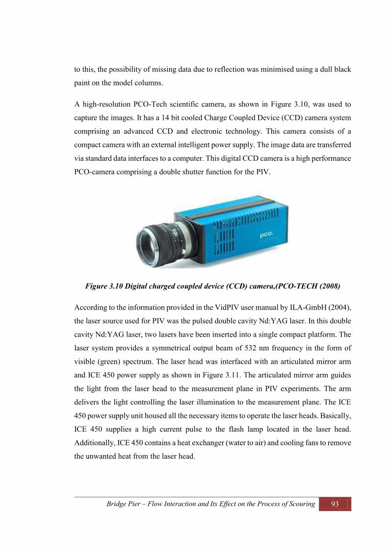
Bridge Pier – Flow Interaction and Its Effect on the Process of Scouring 93
to this, the possibility of missing data due to reflection was minimised using a dull black
paint on the model columns.
A high-resolution PCO-Tech scientific camera, as shown in Figure 3.10, was used to
capture the images. It has a 14 bit cooled Charge Coupled Device (CCD) camera system
comprising an advanced CCD and electronic technology. This camera consists of a
compact camera with an external intelligent power supply. The image data are transferred
via standard data interfaces to a computer. This digital CCD camera is a high performance
PCO-camera comprising a double shutter function for the PIV.
Figure 3.10 Digital charged coupled device (CCD) camera,(PCO-TECH (2008)
According to the information provided in the VidPIV user manual by ILA-GmbH (2004),
the laser source used for PIV was the pulsed double cavity Nd:YAG laser. In this double
cavity Nd:YAG laser, two lasers have been inserted into a single compact platform. The
laser system provides a symmetrical output beam of 532 nm frequency in the form of
visible (green) spectrum. The laser head was interfaced with an articulated mirror arm
and ICE 450 power supply as shown in Figure 3.11. The articulated mirror arm guides
the light from the laser head to the measurement plane in PIV experiments. The arm
delivers the light controlling the laser illumination to the measurement plane. The ICE
450 power supply unit housed all the necessary items to operate the laser heads. Basically,
ICE 450 supplies a high current pulse to the flash lamp located in the laser head.
Additionally, ICE 450 contains a heat exchanger (water to air) and cooling fans to remove
the unwanted heat from the laser head.

Bridge Pier – Flow Interaction and Its Effect on the Process of Scouring 94
Figure 3.11 Laser source and the controlling system: a) laser head with mirrored arm
(ILA-GmbH), and b) ICE450 power supply system (Quantel (2006)
Another important component of the PIV system is its synchronizer, which is a high
precision timing unit acting as an external trigger for both the camera and the laser. It is
controlled by the computer software known as synchronizer control. It dictates the timing
of each image from the CCD camera with a very low jitter down to 0.1 ns so that the PIV
measurement can be conducted at a very precise moment.
3.4 Experimental Procedure and Data Acquisition
3.4.1 Procedure for Fixed Bed Experiments in Flume 1
At the very first step of the experiment, the bed material (sand) with a mean grain size
(d50) of 0.85 mm was placed in the sand recess. With the help of a long straight edged
rectangular wooden bar, the sand in the flume was levelled. On the levelled bed, the initial
bed elevations were checked using a vernier point gauge at random points to ensure the
proper levelling. After levelling the sand bed, column model with diameter (D) of 55 mm
as bridge piers were carefully installed at the centreline of the flume along the
longitudinal direction. The columns were installed in such a way that they were
positioned exactly at the vertical position. The position and the inclination of the columns
were measured using a common measuring tape, bubble level and a tri-square and
adjusted to accurate positions. For acquiring better results from the experiments, the
position and vertical-ness of columns are very important. It can be noted that significant
change in the flow pattern may occur due to column position and orientation disparities.
The next step was to fill the flume with water. Keeping the tailgate in closed condition,
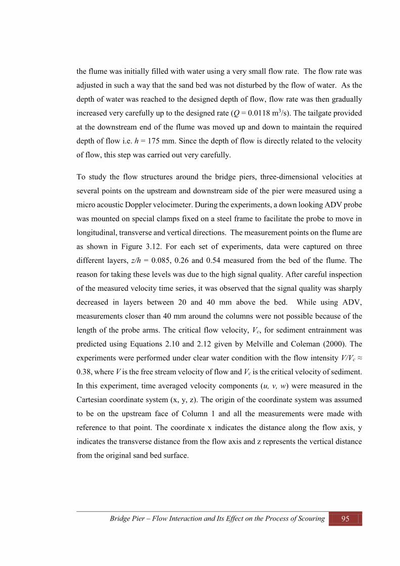
Bridge Pier – Flow Interaction and Its Effect on the Process of Scouring 95
the flume was initially filled with water using a very small flow rate. The flow rate was
adjusted in such a way that the sand bed was not disturbed by the flow of water. As the
depth of water was reached to the designed depth of flow, flow rate was then gradually
increased very carefully up to the designed rate (Q = 0.0118 m3/s). The tailgate provided
at the downstream end of the flume was moved up and down to maintain the required
depth of flow i.e. h = 175 mm. Since the depth of flow is directly related to the velocity
of flow, this step was carried out very carefully.
To study the flow structures around the bridge piers, three-dimensional velocities at
several points on the upstream and downstream side of the pier were measured using a
micro acoustic Doppler velocimeter. During the experiments, a down looking ADV probe
was mounted on special clamps fixed on a steel frame to facilitate the probe to move in
longitudinal, transverse and vertical directions. The measurement points on the flume are
as shown in Figure 3.12. For each set of experiments, data were captured on three
different layers, z/h = 0.085, 0.26 and 0.54 measured from the bed of the flume. The
reason for taking these levels was due to the high signal quality. After careful inspection
of the measured velocity time series, it was observed that the signal quality was sharply
decreased in layers between 20 and 40 mm above the bed. While using ADV,
measurements closer than 40 mm around the columns were not possible because of the
length of the probe arms. The critical flow velocity, Vc, for sediment entrainment was
predicted using Equations 2.10 and 2.12 given by Melville and Coleman (2000). The
experiments were performed under clear water condition with the flow intensity V/Vc ≈
0.38, where V is the free stream velocity of flow and Vc is the critical velocity of sediment.
In this experiment, time averaged velocity components (u, v, w) were measured in the
Cartesian coordinate system (x, y, z). The origin of the coordinate system was assumed
to be on the upstream face of Column 1 and all the measurements were made with
reference to that point. The coordinate x indicates the distance along the flow axis, y
indicates the transverse distance from the flow axis and z represents the vertical distance
from the original sand bed surface.
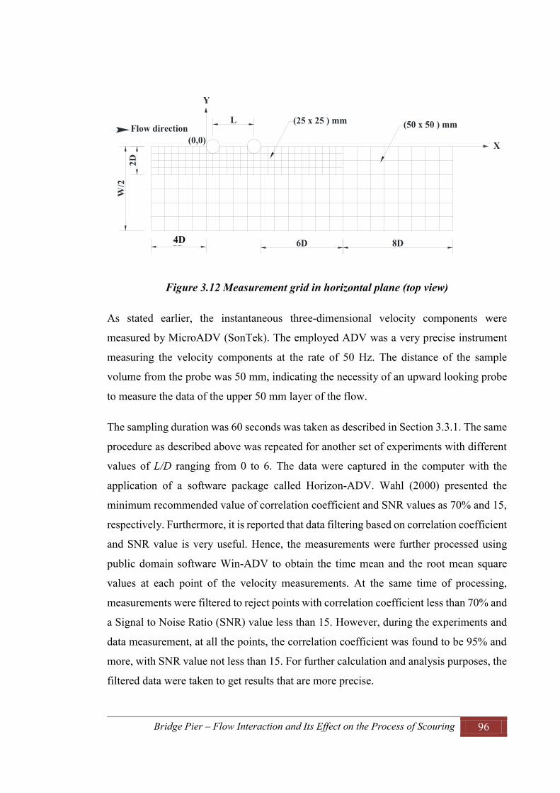
Bridge Pier – Flow Interaction and Its Effect on the Process of Scouring 96
Figure 3.12 Measurement grid in horizontal plane (top view)
As stated earlier, the instantaneous three-dimensional velocity components were
measured by MicroADV (SonTek). The employed ADV was a very precise instrument
measuring the velocity components at the rate of 50 Hz. The distance of the sample
volume from the probe was 50 mm, indicating the necessity of an upward looking probe
to measure the data of the upper 50 mm layer of the flow.
The sampling duration was 60 seconds was taken as described in Section 3.3.1. The same
procedure as described above was repeated for another set of experiments with different
values of L/D ranging from 0 to 6. The data were captured in the computer with the
application of a software package called Horizon-ADV. Wahl (2000) presented the
minimum recommended value of correlation coefficient and SNR values as 70% and 15,
respectively. Furthermore, it is reported that data filtering based on correlation coefficient
and SNR value is very useful. Hence, the measurements were further processed using
public domain software Win-ADV to obtain the time mean and the root mean square
values at each point of the velocity measurements. At the same time of processing,
measurements were filtered to reject points with correlation coefficient less than 70% and
a Signal to Noise Ratio (SNR) value less than 15. However, during the experiments and
data measurement, at all the points, the correlation coefficient was found to be 95% and
more, with SNR value not less than 15. For further calculation and analysis purposes, the
filtered data were taken to get results that are more precise.
(0,0) X
Y
Flow directionL (25 x 25 ) mm (50 x 50 ) mm
2D 6D 8D
2DW
/2
4D

Bridge Pier – Flow Interaction and Its Effect on the Process of Scouring 97
3.4.2 Procedure for Mobile Bed Experiments in Flume 1
In these experiments, three sets of experiments were carried out for different flow
conditions. Preparation of the bed was carried out in a similar way as described in fixed
bed experiments. A set of 34 numbers of experiments using a single column (4
experiments for four different flow conditions) and two in-line circular columns (10
different L/D × 3 flow conditions = 30 experiments) with different spacing were
conducted. The duration of the experiments was taken as 72 to 75 hours because after 75
hours of the test duration, no sediment movement around Column 1 was noticed. The
columns were installed in the flume with different spacing between them (for example
L/D=1, 2, 3, 4, 5, 6, 8, 10 and 12 centre to centre of columns). For each set of column
arrangements, three different flow conditions as shown in Table 3.2 were established. Out
of these experimental tests, four experiments (the single column and two in-line circular
columns with spacing 1D, 2D and 3D) conducted under the flow condition of Test 2 as
shown in Table 3.2 were monitored for the development of scour hole and measurements
were taken at different elapsed times. At the end of each test, the pump was stopped and
all water was carefully drained out from the flume. Measurements of the final bed level
were carried out using a vernier point gauge. The scour depth and scour profiles in the
upstream side and the downstream side of both the columns were measured. The scour
profiles measurements were carried out along the axis of symmetry of the columns and
measurement points were about 20 mm apart. Additionally, the maximum scour depth,
the minimum scour depth, the size of the scour hole and the angle of repose were
measured and recorded for further analysis.
3.4.3 Procedure for Fixed Bed Experiments in Flume 2
In Flume 2, a set of fixed bed experiments were carried out for the study of flow structures
around bridge piers consisting of a single column as well as two in-line circular columns.
A set of 40 numbers (8 different L/D × 5 different Y/D = 40 runs) of experimental runs
were carried out for the same flow conditions with different spacing between the columns.
The model columns (16 mm in diameter) of bridge piers were painted with dull black
paint to minimise the reflection effect during the experiment to avoid the data missing.
The columns were installed on the centre line of the flume at a distance of 2 m from the

Bridge Pier – Flow Interaction and Its Effect on the Process of Scouring 98
inlet section of the flume. The flow rate of 3 l/s was supplied to the flume and the depth
of flow was maintained at 130 mm. The details of flow condition are presented in Table
3.2. Additionally the flume was equipped with apparatus required for the Particle Image
Velocimetry (PIV) as described in Section 3.3.2. The equipment was installed in such a
way that detailed data in the vertical plane could readily be measured. The chances of
capturing missing data were decreased by manipulating the camera distance, laser width
and position of laser head. The laser-guided arm was positioned on the top of the flume
and the laser sheet was projected on the required measurement axis. The camera was
installed in front of the flume perpendicular to the laser sheet. The measurements were
carried out at different vertical planes parallel to the direction of flow as shown in Figure
3.13 i.e. planes at y/D = 0, 1.25, 2.5, 3.75 and 5. For each set of experiment, images were
captured for various spacing between the columns i.e. L/D = 0, 1, 2, 2.5, 3, 4, 5 and 6.
Figure 3.13 Different axes of PIV measurements (top view)
Once the setup was completed, the seeding particles (Polyamide 2070) were added to the
flow. These seeding particles were illuminated in the plane of flow at least twice by means
of a laser within a short time interval. It was assumed that the seeding particles follow the
flow velocity between the two illuminations. The light scattered by seeded particles was
acquired by a high-resolution digital camera. The images acquired from camera were
stored in the computer. The flow field was measured on a grid of interrogation area of the
size 32 × 32 pixels. It can be noted that the displacement of seeding particles between
two consecutive images determines the fluid velocity. To extract displacement
a) Flow Direction
Y/D = 0
Y/D = 2.5
Y/D = 3.75
Y/D = 5.0
Y/D = 1.25
LD D
Column 1 Column 2
(0,0)
Y
XStream wise direction
Tran
sver
se d
irec
tion
b)

Bridge Pier – Flow Interaction and Its Effect on the Process of Scouring 99
information from the PIV recordings, the stored images were processed using a software
package called VidPIV. In the first step of image processing, a spatial calibration was
carried out by generating image mapping to map measurements made from the images in
the pixel unit. The annotation function was used to exclude the mask areas where no
velocity information was present. The cross correlation function was applied to the raw
PIV images to extract the most common particle displacement found between two
interrogations areas. The vector information extracted was further filtered to remove
outliers and interpolated to calculate the missing data. An additional operation was
applied using adaptive cross correlation to achieve a higher accuracy improving the
correlation coefficient. Vector filters were reapplied, followed by interpolation and
finally the vector maps were derived as vector magnitudes. These vector magnitudes were
extracted and saved for further analysis of the flow field.
3.5 Summary
A series of laboratory experiments have been conducted on flow structures and scour
around bridge piers in the hydraulics laboratory at the University of Technology, Sydney.
Two different sized flumes were used for the experimental tests. Flume 1 is 19 m long,
0.61 m wide and 0.61 m deep. At the working section of the flume, there is section in the
form of a recess, which is 5.00 m long and 0.15 m deep, located at 9.0 m downstream
from the flume inlet section. Another flume with a smaller size (Flume 2) with dimensions
of 6 m long, 0.25 m wide and 0.25 m deep was used for the study of flow structures
around the bridge piers under fixed bed condition using Particle Image Velocimetry. Both
flumes were equipped with a flow meter, a regulating gate and a pump. An
electromagnetic flow meter was used to measure the flow rate of water in the flume. The
scour depth was measured using a vernier point gauge with least count of 0.05 mm. This
point gauge was mounted on the flume in such a way that it could move in all the three
directions.
The model columns used for Flume 1 were circular pipes with an external diameter of 55
mm, while for Flume 2 the column diameter was 16 mm. The diameters of the columns
were selected in such a way that there was no contraction effect on the depth of the scour.
For this reason, the flume width to the column diameter ratio was checked to be greater

Bridge Pier – Flow Interaction and Its Effect on the Process of Scouring 100
than 10. Uniformly graded non-cohesive sand of mean grain size (d50) of 0.85 mm was
used as a bed material. The size of the sand was determined in such a way that there was
no grain size effect on the scour depth. It was determined using the design criteria
developed by Ettema (1976).
All of the experimental tests were conducted under clear water flow condition with
different values of the critical velocity ratio (V/Vc). The critical velocity of flow was
determined based on the relationships given by Melville and Coleman (2000). For each
flow condition, different tests were carried out including a single column, and two in-line
circular columns with different spacing between them (L/D = 0 to 6). Altogether 64 runs
(28 runs for ADV method + 40 runs for PIV method) of fixed bed experiments were
carried out for the study of flow structures. Velocity was measured using ADV apparatus
and PIV measurement techniques. The ADV apparatus was used to measure the three
dimensional velocity components in the horizontal plane and the PIV method was used
to measure the two dimensional velocity components in vertical planes. Additionally, 34
numbers of moveable bed experiments under different flow conditions were carried out
for the study of scour depth.
Bridge Pier – Flow Interaction and Its Effect on the Process of Scouring 101
CHAPTER 4
RESULTS AND DISCUSSION ON FLOW STRUCTURE
4.1 Introduction
4.2 Previous Investigations on Flow around Bridge Piers
4.3 Flow around Bridge Piers in Horizontal Plane
4.4 Flow around Bridge Piers in Vertical Plane
4.5 Bursting Phenomenon and Quadrant Analysis
4.6 Summary

Bridge Pier – Flow Interaction and Its Effect on the Process of Scouring 102
4. RESULTS AND DISCUSSION ON FLOW STRUCTURE
4.1 Introduction
The flow around bridge piers is one of the most important topics of interest to hydraulic
engineers and designers because it will lead to an in-depth understanding of flow and its
consequences. As reported by Ahmed and Rajaratnam (1998), numerous studies have
been conducted since the late 1950s to understand the flow structure around bridge piers
and its relationship with the local scour. However, the complex three dimensional flow
structure and its interaction with the sediment transport create great difficulties in
analysing the problems. Menna and Pierce (1988), Ahmed and Rajaratnam (1998) and
Dey and Raikar (2007) provided a comprehensive understanding of three dimensional
turbulent flow structure and the concept of mechanism of scouring process to predict the
depth of the scour hole within a high level of precision.
Many tests have been conducted to study the flow structure around a single column and
two in-line circular columns with varying spacing between them. An acoustic Doppler
velocimeter (ADV) was employed to measure the velocity components of flow in three
different horizontal planes, while particle image velocimetry (PIV) was used to measure
instantaneous velocity in different vertical planes parallel to the direction of flow. The
results are analysed and presented in this chapter.
4.2 Previous Investigations on Flow around Bridge Piers
As presented in Section 2.4, many researchers have conducted extensive investigations
on flow structures. A brief review to highlight the main findings of the investigations is
presented in this section:
Melville and Raudkivi (1977b) conducted an experimental study on flow around a
circular cylinder under flat bed and deformed bed conditions. They measured the flow,
turbulence intensity and bed shear stress distribution around the cylinder using a hot film
anemometer. The hydrogen bubble technique was used to obtain the flow pattern. Their
experiments disclosed that there was the presence of spiral flow in the form of necklace
vortices at the base of the cylinder. The weaker necklace vortices and the lower level of

Bridge Pier – Flow Interaction and Its Effect on the Process of Scouring 103
turbulence intensity were reported at equilibrium scour conditions compared to the flat
bed condition.
Menna and Pierce (1988) presented the experimental results of the mean flow structure
of the upstream and surrounding flow around a teardrop shaped cylinder. Measurements
included the mean velocity, Reynolds stresses, turbulent kinetic energy, floor pressure,
and wall shear stress. It was observed that the flow was continuously turned down to the
wall and its direction near the wall was significantly different from that of the wall shear
stress. It was also reported that the boundary layer thickness did not change significantly
around the cylinder and the flow observed to be accelerated within the undisturbed
boundary layer.
Ahmed and Rajaratnam (1998) conducted an experimental study of the flow and bed
shear stress field around a circular cylinder on different types of bed conditions. The
experiments were carried out on smooth and rough bed surfaces under flat bed and
scoured bed conditions. That study showed the effects of bed roughness and the presence
of scour hole on the flow field. It was concluded that the bed roughness induced a steeper
pressure gradient resulting in strong down-flow in front of the pier. The maximum down-
flow in the absence of scour hole was reported approximately 35% of the approach flow.
Additionally they concluded that the magnitude of the bed shear stress was increased due
to the bed roughness. It was noticed in the experiments that the skewing of the flow near
the bed was resisted by the bed roughness.
Unger and Hager (2007) conducted an experimental study to investigate the internal flow
features around circular bridge piers using particle image velocimetry system. They
performed the study over a wide range of Reynolds number (5 × 10⁴ – 3.5 × 10⁶) and
visualised the flow pattern in several horizontal and vertical planes. The temporal
evolution of vertical flow in front of the pier and the horseshoe vortex inside the scour
hole were investigated measuring the velocity and vorticity profiles. It was identified that
the horseshoe vortex system is the main reason for the growth of scour hole. Based on
the experimental data, they derived an empirical relation for the temporal evolution of the
size and the shape of the primary vortex of the horseshoe vortex system. Additionally,

Bridge Pier – Flow Interaction and Its Effect on the Process of Scouring 104
they found the slight variation of the strength of down flow and the position of the
stagnation point during the scour process.
Beheshti and Ataie-Ashtiani (2010) performed an experimental investigation on the three
dimensional flow field around a complex bridge pier placed on a rough fixed bed. The
pier model consisted of a column, a pile cap, and a 2×4 pile group. The instantaneous
three dimensional velocity components were measured using an ADV. The results were
presented in the form of profile and contour plots of three dimensional velocity
components, turbulent intensity components, turbulent kinetic energy, and Reynolds
stresses. In addition to this, the velocity vectors were presented and discussed at different
vertical and horizontal planes. It was reported that the approaching boundary layer at the
upstream of the bridge piers separated in two vertical directions, with an upward flow
towards the column and a contracted flow in the downward direction towards the pile.
They found that the main features responsible for the sediment entrainment were the
contracted flow below the pile cap and towards the piles, a strong down flow along the
side of the piers at the upstream region, and a vortex flow behind the pier and
amplification of the turbulence intensity along the side of the piers at the downstream
side.
Kumar and Kothyari (2012b) performed an experimental study on the flow pattern and
the three dimensional turbulence characteristics around the circular uniform and the
compound piers in the presence of scour hole. Four sets of experimental tests were carried
out under the clear water flow condition using a uniform circular pier and circular
compound pier. The flow field was observed in the pre-developed scour hole and three
dimensional velocity components were measured using an ADV. Detailed measurement
of time averaged velocities, turbulence intensities and Reynolds shear stresses at eight
different vertical profiles for various radial distances from the centre of the piers were
examined. In that study, the diameter of the principal vortex at upstream of the pier was
expressed in terms of diameter of the pier. It was noticed that the profile of flow velocity,
turbulence intensities and Reynolds shear stresses around each of the pier models at
different vertical planes were more or less similar. However, the measurements close to
the piers showed significant changes in the vertical profile of flow parameters.

Bridge Pier – Flow Interaction and Its Effect on the Process of Scouring 105
An experimental study on turbulence flow and sediment entrainment around a bridge pier
was conducted by Izadinia et al. (2013). They reported that the maximum velocity
occurred at the edge of the scour hole and the velocity profile became normal outside the
scour hole. At the downstream side of the pier, the secondary currents were found more
significant because of the occurrence of maximum velocity near the bed. The observed
turbulence intensity component in the transverse direction was larger in the downstream
side. Similarly, vertical Reynolds stress (u′w′) was reported stronger at the downstream
side of a pier. They concluded that there was occurrence of heavily fluctuating Reynolds
stress at the downstream side and unsteady shedding wake vortices due to flow
separation.
Recently, Ataie-Ashtiani and Aslani-Kordkandi (2013) conducted an experimental study
on the flow field around a single column and two in-line columns with the spacing of 3D.
That study provided a comparison between the flow pattern around the single pier and
two in-line circular columns. During the experiments, the model columns were installed
on a moderately rough flatbed laboratory flume. The results were time average velocity
components, turbulence intensity components, turbulent kinetic energy, and Reynolds
shear stresses and were presented graphically in the form of contour and profile. The
power spectra analysis of instantaneous velocity measurements at different points were
also presented in this study. It was reported that the results from the experiments showed
significant changes in the flow structure, particularly in the near wake region, due to the
presence of the downstream pier. Within the gap between the two columns, a stronger up-
flow and weaker transverse deflection were formed in comparison with that of the single
column case. Sheltering effect was noticed due to which the velocity of flow approaching
the downstream pier was decreased to 20% to 30% of the approach mean velocity.
Comparing with the results of single pier, considerable decrease in turbulent intensities
and turbulent kinetic energy were noticed around two in-line circular columns. Decrease
in the strength of vortex structure in the wake of the two-column case in comparison with
the single column case was reported as a result of the power spectra analysis.
It is clear from the above review that most of the investigations on flow structure were
based on the bridge piers with a single circular column. Apparently, only a few studies
were associated with two in-line circular columns. However, effects of spacing between

Bridge Pier – Flow Interaction and Its Effect on the Process of Scouring 106
two in-line columns on flow structures were not well investigated. Hence, in the present
study, an in-depth investigation on the effect of spacing between two in-line circular
columns on flow structures has been analysed and compared with the findings from
previous investigations.
4.3 Flow around the Bridge Piers in Horizontal Plane
In this study, the data acquisition around the bridge piers in horizontal planes was carried
out as described in the Section 3.4.1. The three dimensional instantaneous velocity
components were measured using an ADV in three different horizontal layers. The first
layer was close to the bed with Z/h = 0.09, the second layer was at the depth with Z/h =
0.26 and the measurement at the third layer was carried out at the depth with Z/h = 0.54.
The captured data were processed and analysed using Win-ADV software. For the sake
of simplicity, in the case of two in-line circular columns, the column at the upstream side
is denoted as Column 1 (or C1) and the column at the downstream side is denoted as
Column 2 (or C2). The measurements were carried out in Cartesian coordinate system
provided that the origin is located at the upstream face of the Column 1. Different
notations associated with bridge pier arrangement, used in this thesis, are shown in Figure
4.1. In the figure, X and Y represent the axes along streamwise and transverse direction,
respectively; whereas D and L represent the diameter of the column and the centre-to-
centre distance between two in-line circular columns.
Figure 4.1 Definition sketch of the bridge piers arrangement
(0,0) X
Y
D DL
Column 1 Column 2
Flow direction

Bridge Pier – Flow Interaction and Its Effect on the Process of Scouring 107
Figure 4.2 Schematic diagram of different axis of data analysis in horizontal planes
The results on the flow field and the turbulence characteristics of the flow around bridge
piers and the effects of spacing between two in-line circular columns are presented in the
following subsections. The processed and analysed data are presented in contour and
profile plots for velocity components (u, v, and w), velocity fluctuation components (u′,
v′ and w′), turbulence intensity components (TIu, TIv and TIw), turbulent kinetic energy
(TKE) and Reynolds stresses. Comparisons have been carried out for different
combinations including the single column and the double columns with various L/D ratios
(i.e. L/D = 1.5, 2, 3, 4, 5 and 6). In addition, for each column arrangement, the three
dimensional data along three different lines parallel to the flow direction have been
extracted, as shown in Figure 4.2.
4.3.1 Flow Pattern
Vector plots and the stream line plots as shown in Figure 4.3 for the single column case
and Figure 4.4 for two in-line circular columns case with L/D = 3 clearly represent the
flow patterns around the bridge piers. The detailed figures of velocity vectors and
streamline plots in planes Z/h = 0.26 and 0.54 for different values of L/D are presented in
Appendices A.1.1 and A.1.2. In the vector diagram, the length of the vector gives the
resultant magnitude of velocity components u and v given by , the direction is
clearly represented by the inclination of the vectors. For the condition of no piers, it is
observed that there is not any deflection in velocity vectors and the magnitude of the
vectors is uniform throughout the flow field. When a column was added to the system,
flow started deflecting from its original direction. It was common to all the cases that the
flow pattern at the upstream side of a column was similar, while at the downstream side
D D
D D
L
Y/D = 0
Y/D = 1
Y/D = 2
Column 1 Column 2
Flow DirectionA B
0.9
1.8
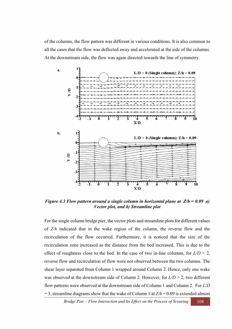
Bridge Pier – Flow Interaction and Its Effect on the Process of Scouring 108
of the columns, the flow pattern was different in various conditions. It is also common to
all the cases that the flow was deflected away and accelerated at the side of the columns.
At the downstream side, the flow was again directed towards the line of symmetry.
Figure 4.3 Flow pattern around a single column in horizontal plane at Z/h = 0.09 a) Vector plot, and b) Streamline plot
For the single column bridge pier, the vector plots and streamline plots for different values
of Z/h indicated that in the wake region of the column, the reverse flow and the
recirculation of the flow occurred. Furthermore, it is noticed that the size of the
recirculation zone increased as the distance from the bed increased. This is due to the
effect of roughness close to the bed. In the case of two in-line columns, for L/D < 2,
reverse flow and recirculation of flow were not observed between the two columns. The
shear layer separated from Column 1 wrapped around Column 2. Hence, only one wake
was observed at the downstream side of Column 2. However, for L/D > 2, two different
flow patterns were observed at the downstream side of Column 1 and Column 2. For L/D
= 3, streamline diagrams show that the wake of Column 1 at Z/h = 0.09 is extended almost
a.
b.

Bridge Pier – Flow Interaction and Its Effect on the Process of Scouring 109
throughout the gap. The shear layer, which separated from Column 1 re-attached on the
upstream side of Column 2. According to the description of flow regime made on Section
2.4.2, it is called the re-attachment regime, which is principally characterised by
formation and shedding of eddies in the gap. As the distance from the bed increased, the
shear layer, which separated from Column 1 moved towards the downstream side of
Column 2. This nature of flow indicates that there is no vortex shedding between the two
columns. Further increase in spacing results in the flow separation at a distance about 2D
measured from the face of Column 1. There was formation of vortex shedding at the
downstream side of both Column 1 and Column 2. As described in Section 2.4.2, it is
called the co-shedding regime. In this regime, both the columns undergo vortex shedding
of the same frequency and produce weaker vortices behind Column 2 than that in the case
of L/D < 3. This is attributed to the disturbance of vortex shedding of Column 1 to the
vortex shedding behind Column 2.
Figure 4.4 Flow pattern around two columns with L/D = 3 in horizontal plane at Z/h = 0.09 a) Vector plot, and b) Streamline plot
a.
b.
L/D = 3; Z/h = 0.09
L/D = 3; Z/h = 0.09
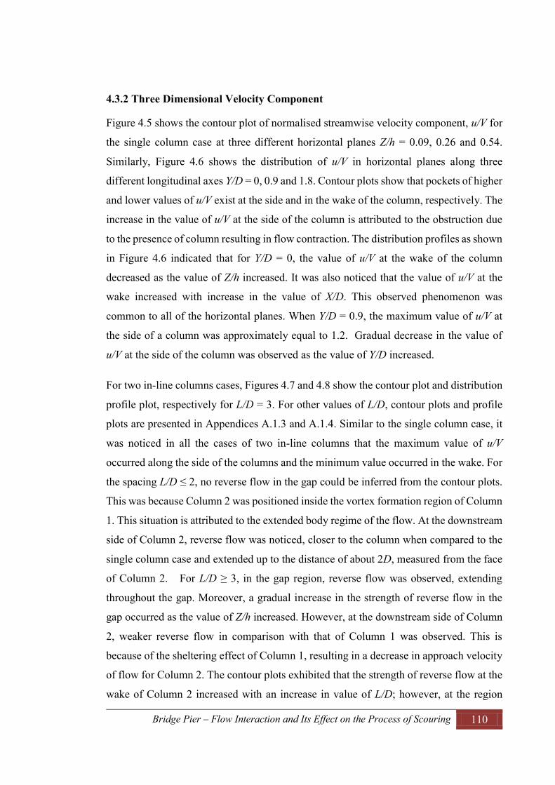
Bridge Pier – Flow Interaction and Its Effect on the Process of Scouring 110
4.3.2 Three Dimensional Velocity Component
Figure 4.5 shows the contour plot of normalised streamwise velocity component, u/V for
the single column case at three different horizontal planes Z/h = 0.09, 0.26 and 0.54.
Similarly, Figure 4.6 shows the distribution of u/V in horizontal planes along three
different longitudinal axes Y/D = 0, 0.9 and 1.8. Contour plots show that pockets of higher
and lower values of u/V exist at the side and in the wake of the column, respectively. The
increase in the value of u/V at the side of the column is attributed to the obstruction due
to the presence of column resulting in flow contraction. The distribution profiles as shown
in Figure 4.6 indicated that for Y/D = 0, the value of u/V at the wake of the column
decreased as the value of Z/h increased. It was also noticed that the value of u/V at the
wake increased with increase in the value of X/D. This observed phenomenon was
common to all of the horizontal planes. When Y/D = 0.9, the maximum value of u/V at
the side of a column was approximately equal to 1.2. Gradual decrease in the value of
u/V at the side of the column was observed as the value of Y/D increased.
For two in-line columns cases, Figures 4.7 and 4.8 show the contour plot and distribution
profile plot, respectively for L/D = 3. For other values of L/D, contour plots and profile
plots are presented in Appendices A.1.3 and A.1.4. Similar to the single column case, it
was noticed in all the cases of two in-line columns that the maximum value of u/V
occurred along the side of the columns and the minimum value occurred in the wake. For
the spacing L/D ≤ 2, no reverse flow in the gap could be inferred from the contour plots.
This was because Column 2 was positioned inside the vortex formation region of Column
1. This situation is attributed to the extended body regime of the flow. At the downstream
side of Column 2, reverse flow was noticed, closer to the column when compared to the
single column case and extended up to the distance of about 2D, measured from the face
of Column 2. For L/D ≥ 3, in the gap region, reverse flow was observed, extending
throughout the gap. Moreover, a gradual increase in the strength of reverse flow in the
gap occurred as the value of Z/h increased. However, at the downstream side of Column
2, weaker reverse flow in comparison with that of Column 1 was observed. This is
because of the sheltering effect of Column 1, resulting in a decrease in approach velocity
of flow for Column 2. The contour plots exhibited that the strength of reverse flow at the
wake of Column 2 increased with an increase in value of L/D; however, at the region
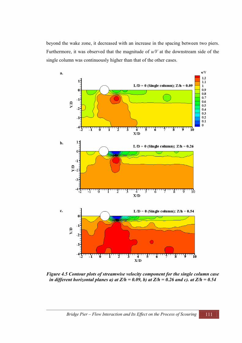
Bridge Pier – Flow Interaction and Its Effect on the Process of Scouring 111
beyond the wake zone, it decreased with an increase in the spacing between two piers.
Furthermore, it was observed that the magnitude of u/V at the downstream side of the
single column was continuously higher than that of the other cases.
Figure 4.5 Contour plots of streamwise velocity component for the single column case in different horizontal planes a) at Z/h = 0.09, b) at Z/h = 0.26 and c). at Z/h = 0.54
a.
b.
c.
Y/D

Bridge Pier – Flow Interaction and Its Effect on the Process of Scouring 112
Figure 4.6 Profile plots of streamwise velocity component for the single column case in different horizontal planes along three different longitudinal axes a) at Z/h = 0.09,
b) at Z/h = 0.26 and c). at Z/h = 0.54
a.
b.
c.
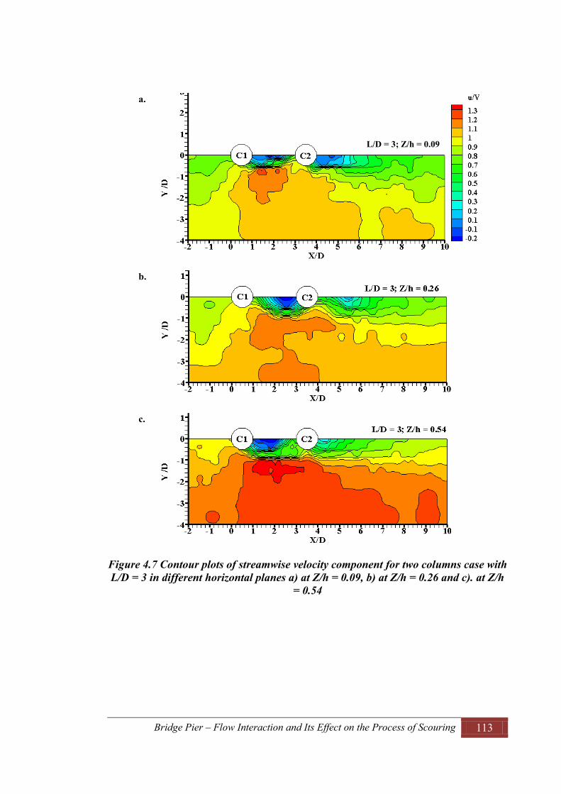
Bridge Pier – Flow Interaction and Its Effect on the Process of Scouring 113
Figure 4.7 Contour plots of streamwise velocity component for two columns case with L/D = 3 in different horizontal planes a) at Z/h = 0.09, b) at Z/h = 0.26 and c). at Z/h
= 0.54
a.
b.
c.
L/D = 3; Z/h = 0.09

Bridge Pier – Flow Interaction and Its Effect on the Process of Scouring 114
Figure 4.8 Profile plots of the streamwise velocity component for two-column case with L/D = 3 in different horizontal planes along three different longitudinal axes a)
at Z/h = 0.09, b) at Z/h = 0.26 and c). at Z/h = 0.54
The normalised transverse velocity components, v/V for the single column case and the
two-column case L/D = 3 are presented in contour plots as in Figures 4.9 and 4.10,
respectively. Similarly, the distribution of v/V along three different longitudinal axes Y/D
= 0, 0.9 and 1.8 for the single column case and the two-column case with L/D = 3 are
a.
b.
c.
-4 -2 0 2 4 6 8 10 12 14-0.5
0
0.5
1
1.5
X/D
u/V
L/D = 3; Z/h = 0.09
Y/D = 0Y/D = 0.9Y/D = 1.8
-4 -2 0 2 4 6 8 10 12 14-0.5
0
0.5
1
1.5
X/D
u/V
L/D = 3; Z/h = 0.26
Y/D = 0Y/D = 0.9Y/D = 1.8
-4 -2 0 2 4 6 8 10 12 14-0.5
0
0.5
1
1.5
X/D
u/V
L/D = 3; Z/h = 0.54
Y/D = 0Y/D = 0.9Y/D = 1.8

Bridge Pier – Flow Interaction and Its Effect on the Process of Scouring 115
presented in Figures 4.11 and 4.12, respectively. The detailed contour plots and profile
plots for different values of L/D at three different horizontal planes at Z/h = 0.09, 0.26
and 0.54 are presented in Appendices A.1.5 and A.1.6.
Figure 4.9 Contour plots of transverse velocity component for the single column case in different horizontal planes a) at Z/h = 0.09, b) at Z/h = 0.26 and c). at Z/h = 0.54
The contour plots for the single column case in Figure 4.9 indicate that the pocket of
higher value of negative v/V happens at the upstream side near the zone of shear layer
separation. The negative value of v/V indicates the deviation of flow away from the
a.
b.
c.
Y/D

Bridge Pier – Flow Interaction and Its Effect on the Process of Scouring 116
column. At the downstream side, a positive value of v/V was observed i.e. the flow
converged in the wake of a column. The magnitude of v/V in the wake near the bed was
the highest and it decreased as the distance from the bed increased.
Figure 4.10 Profile plots of transverse velocity component for the single column case in different horizontal planes along three different longitudinal axes a) at Z/h = 0.09,
b) at Z/h = 0.26 and c). at Z/h = 0.54
a.
b.
c.
-4 -2 0 2 4 6 8 10 12 14-0.4
-0.2
0
0.2
0.4
X/D
v/V
L/D = 0 (Single column); Z/h = 0.09
Y/D = 0Y/D = 0.9Y/D = 1.8

Bridge Pier – Flow Interaction and Its Effect on the Process of Scouring 117
Figure 4.11 Contour plots of transverse velocity component for the two-column case with L/D = 3 in different horizontal planes a) at Z/h = 0.09, b) at Z/h = 0.26 and c). at
Z/h = 0.54
a.
b.
c.
3

Bridge Pier – Flow Interaction and Its Effect on the Process of Scouring 118
Figure 4.12 Profile plots of transverse velocity component for the two-column case with L/D = 3 in different horizontal planes along three different longitudinal axes a)
at Z/h = 0.09, b) at Z/h = 0.26 and c). at Z/h = 0.54
a.
b.
c.
-4 -2 0 2 4 6 8 10 12 14-0.4
-0.2
0
0.2
0.4
X/D
v/V
L/D = 3; Z/h = 0.09
Y/D = 0Y/D = 0.9Y/D = 1.8
-4 -2 0 2 4 6 8 10 12 14-0.4
-0.2
0
0.2
0.4
X/D
v/V
L/D = 3; Z/h = 0.26
Y/D = 0Y/D = 0.9Y/D = 1.8
-4 -2 0 2 4 6 8 10 12 14-0.4
-0.2
0
0.2
0.4
X/D
v/V
L/D = 3; Z/h = 0.54
Y/D = 0Y/D = 0.9Y/D = 1.8

Bridge Pier – Flow Interaction and Its Effect on the Process of Scouring 119
For the two in-line columns case with L/D ≤ 2, the minimum and maximum values of v/V
were similar to those of the single column case. In the gap between the two columns, no
deflection of the flow was noticed. The contour plots indicated that the pocket of higher
values of v/V occurred at the downstream side of Column 2. Furthermore, the value of
v/V was stronger in the upper level than near the bed. When L/D = 3 at Z/h = 0.09, a
higher value of v/V was observed in the gap, which decreased as the value of Z/h
increased. This can be due to the generation of the re-attachment regime close to the bed.
However, for the upper level, the shear layer separated from Column 1 converged at the
downstream side of Column 2, resulting in a small deflection of flow inside the gap.
Additionally, the figures reveal that the observed transverse velocity in the downstream
side of Column 2 is stronger than that of the case L/D < 2. For L/D > 3, similar results
can be seen from the contour plots. However, the pocket of higher value of v/V occurred
close to Column 1 in its wake. As the flow approached Column 2, the value of v/V became
approximately equal to 0.
The contour plots of normalised velocity component, w/V for the single column and two
in-line columns with L/D = 3 are shown in Figures 4.13 and 4.15, respectively in three
different horizontal planes at Z/h = 0.09, 0.26 and 0.54. Figures 4.14 and 4.16 show the
distribution of w/V along three different longitudinal axes at Y/D = 0, 0.9 and 1.8 in
horizontal planes for single column and two columns with L/D = 3 respectively. Contour
plots and profile plots for other values of L/D in different horizontal planes are presented
in Appendices A.1.7 and A.1.8.

Bridge Pier – Flow Interaction and Its Effect on the Process of Scouring 120
Figure 4.13 Contour plots of vertical velocity component for the single column case in different horizontal planes a) at Z/h = 0.09, b) at Z/h = 0.26 and c). at Z/h = 0.54
b.
c.
Y/D

Bridge Pier – Flow Interaction and Its Effect on the Process of Scouring 121
Figure 4.14 Profile plots of vertical velocity component for the single column case in different horizontal planes along three different longitudinal axes a) at Z/h = 0.09, b)
at Z/h = 0.26 and c). at Z/h = 0.54
For the single column case as shown in Figure 4.13, a negative value of w/V was observed
close to the column at the upstream side. It is clear from Figure 4.14 that at the upstream
side of a column, the negative value of w/V increases as the flow approaches the column.
The negative value of w/V is indication of the down flow, which is due to the pressure
a.
b.
c.

Bridge Pier – Flow Interaction and Its Effect on the Process of Scouring 122
difference at the stagnation point. The occurrence of down flow was common to all the
cases of two in-line columns. Furthermore, the profile plots for different cases indicate
that the down flow is stronger close to the bed than that in the upper levels. At the
downstream side of the columns, a positive value of w/V is observed i.e. an up flow was
noticed for all cases. In the case of the single column, the pocket of higher values of w/V
occurred close to the bed, while the extent of up flow increased as the value of Z/h
increased.
Figure 4.15 Contour plots of vertical velocity component for the two-column case with L/D = 3 in different horizontal planes a) at Z/h = 0.09, b) at Z/h = 0.26 and c). at
Z/h = 0.54
a.
b.
c.
L/D = 3; Z/h = 0.09

Bridge Pier – Flow Interaction and Its Effect on the Process of Scouring 123
Figure 4.16 Profile plots of vertical velocity component for the two-column case with L/D = 3 in different horizontal planes along three different longitudinal axes a) at
Z/h = 0.09, b) at Z/h = 0.26 and c). at Z/h = 0.54
In the case of two in-line columns, for L/D ≤ 2, the weak up flow were noticed inside the
gap. As the spacing between two columns increased, intensity of up flow increased in the
wake of Column 1. At the downstream side of Column 2, weaker up flow than that of
single column was observed close to the bed. However, a small down flow was noticed
behind Column 2 at mid depth. Similar results were reported by Ataie-Ashtiani and
a.
b.
c.
-4 -2 0 2 4 6 8 10 12 14-0.1
0
0.1
0.2
0.3
0.4
X/D
w/V
L/D = 3; Z/h = 0.09
Y/D = 0Y/D = 0.9Y/D = 1.8
-4 -2 0 2 4 6 8 10 12 14-0.1
0
0.1
0.2
0.3
0.4
X/D
w/V
L/D = 3; Z/h = 0.26
Y/D = 0Y/D = 0.9Y/D = 1.8
-4 -2 0 2 4 6 8 10 12 14-0.1
0
0.1
0.2
0.3
0.4
X/D
w/V
L/D = 3; Z/h = 0.54
Y/D = 0Y/D = 0.9Y/D = 1.8

Bridge Pier – Flow Interaction and Its Effect on the Process of Scouring 124
Aslani-Kordkandi (2013). It can be clearly seen from the contour plots for L/D ≥ 3 that,
as the flow approaches the Column 2, intensity of up flow decreases. On the other hand,
the down flow at the upstream side of Column 2 interacts with the up flow close to the
bed and hence the development of the horseshoe shoe vortex was not expected in front of
Column 2.
4.3.3 Turbulence Intensity
Figure 4.17 Contour plots of streamwise turbulence component for the single column case in different horizontal planes a) at Z/h = 0.09, b) at Z/h = 0.26 and c). at Z/h =
0.54
Three dimensional turbulence intensity components in the streamwise direction (TIu), in
the transverse direction (TIv), and in the vertical direction (TIw) have been obtained by
calculating the root mean square values of the velocity fluctuation components u′, v′ and
a.
b.
c.
Y/D

Bridge Pier – Flow Interaction and Its Effect on the Process of Scouring 125
w′, respectively. To analyse the turbulence intensity, it has been normalised using the free
stream velocity (V). The normalised turbulence intensity components TIu/V, TIv/V and
TIw/V are presented in contour plots and profile plots in different horizontal planes.
Figure 4.18 Profile plots of streamwise turbulence intensity component for the single column case in different horizontal planes along three different longitudinal axes a)
at Z/h = 0.09, b) at Z/h = 0.26 and c). at Z/h = 0.54
a.
b.
c.
-4 -2 0 2 4 6 8 10 12 140.05
0.1
0.15
0.2
0.25
0.3
0.35
X/D
TIu/
VL/D = 0 (Single column); Z/h = 0.09
Y/D = 0Y/D = 0.9Y/D = 1.8
-4 -2 0 2 4 6 8 10 12 140.05
0.1
0.15
0.2
0.25
0.3
0.35
X/D
TIu/
V
L/D = 0 (Single column); Z/h = 0.26
Y/D = 0Y/D = 0.9Y/D = 1.8
-4 -2 0 2 4 6 8 10 12 140.05
0.1
0.15
0.2
0.25
0.3
0.35
X/D
TIu/
V
L/D = 0 (Single column); Z/h = 0.54
Y/D = 0Y/D = 0.9Y/D = 1.8

Bridge Pier – Flow Interaction and Its Effect on the Process of Scouring 126
Figure 4.19 Contour plots of streamwise turbulence intensity component for the two-column case with L/D = 3 in different horizontal planes a) at Z/h = 0.09, b) at Z/h =
0.26 and c). at Z/h = 0.54
Figures 4.17 and 4.19 show the contour and profile plots, respectively for the single
column case in three different horizontal planes at Z/h = 0.09, 0.26 and 0.54. The profile
plots, shown in Figures 4.18 and 4.20, are generated along three different longitudinal
axes at Y/D = 0, 0.9 and 1.8. The figures illustrate that higher values of TIu/V are observed
in the wake of a column and it is common to all the horizontal planes. However, the
magnitude of TIu/V is observed higher at upper levels than at levels close to the bed. For
two in-line columns cases, contour plots and profile plots are presented in Figures 4.19
and 4.20, and Appendices B.1.1 and B.1.2. The results indicated that for L/D ≤ 2, the
pocket of higher value of TIu/V happened in the wake of Column 2. When L/D = 3, a
b.
c.
3
a.

Bridge Pier – Flow Interaction and Its Effect on the Process of Scouring 127
higher value of TIu/V close to the bed was observed in the wake of both columns with
approximately the same intensity. The value of TIu/V increased as the value of Z/h
increased. Furthermore, the figures exhibit that the value of TIu/V in the gap is higher
than that behind Column 2.
Figure 4.20 Profile plots of streamwise turbulence intensity component for the two-column case with L/D = 3 in different horizontal planes along three different
longitudinal axes a) at Z/h = 0.09, b) at Z/h = 0.26 and c). at Z/h = 0.54
a.
b.
c.
-4 -2 0 2 4 6 8 10 12 140.1
0.15
0.2
0.25
0.3
0.35
X/D
TIu/
V
L/D = 3; Z/h = 0.09
Y/D = 0Y/D = 0.9Y/D = 1.8
-4 -2 0 2 4 6 8 10 12 140.1
0.15
0.2
0.25
0.3
0.35
X/D
TIu/
V
L/D = 3; Z/h = 0.26
Y/D = 0Y/D = 0.9Y/D = 1.8
-4 -2 0 2 4 6 8 10 12 140.1
0.15
0.2
0.25
0.3
0.35
X/D
TIu/
V
L/D = 3; Z/h = 0.54
Y/D = 0Y/D = 0.9Y/D = 1.8

Bridge Pier – Flow Interaction and Its Effect on the Process of Scouring 128
Figure 4.21 Contour plots of transverse turbulence intensity component for the single column case in different horizontal planes a) at Z/h = 0.09, b) at Z/h = 0.26 and c). at
Z/h = 0.54
The distribution of normalised components of turbulence intensity in the transverse
direction, TIv/V in contour plots are shown in Figures 4.21, Figure 4.22 and Appendix
B.1.3 and in profile plots along three different longitudinal axes are shown in Appendix
B.1.4. For the single column case, the contour plots, shown in Figure 4.21indicate that
the maximum value of TIv/V occurs in the wake of the column, which is approximately
equal to 0.6. Comparing this results with the maximum value of TIu/V, it can be seen that
the maximum value of TIv/V is about 2 times higher than that of TIu/V. Furthermore, it
a.
b.
c.
Y/D

Bridge Pier – Flow Interaction and Its Effect on the Process of Scouring 129
can be clearly seen from the contour plots and profile plots that the value of TIv/V
increases as the distance from the bed increases towards the free surface. Additionally the
contour plots, depicted in Figure 4.21a, close to the bed at Z/h = 0.09 exhibits that the
upstream portion of column experiences a small pocket of higher value of TIv/V. The
reason behind this could be the effect of bed roughness.
Figure 4.22 Contour plots of transverse turbulence intensity component for the two-column case with L/D = 3 in different horizontal planes a) at Z/h = 0.09, b) at Z/h =
0.26 and c). at Z/h = 0.54
Figure 4.23 shows the contour plots of TIv/V for two in-line columns with L/D = 3 at
horizontal planes. In order to compare the results, other figures for different values of L/D
are referenced from Appendix B.1.3. Referring to the contour plots for two in-line
b.
c.
3a.
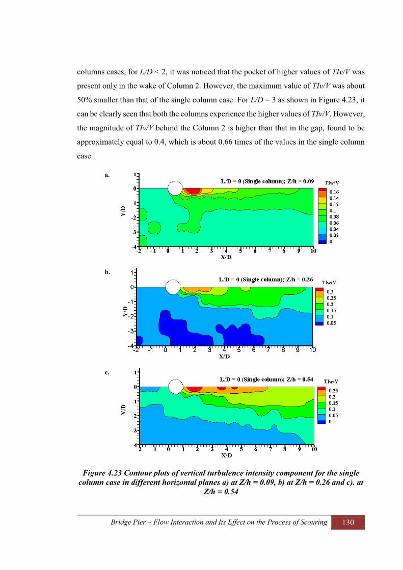
Bridge Pier – Flow Interaction and Its Effect on the Process of Scouring 130
columns cases, for L/D < 2, it was noticed that the pocket of higher values of TIv/V was
present only in the wake of Column 2. However, the maximum value of TIv/V was about
50% smaller than that of the single column case. For L/D = 3 as shown in Figure 4.23, it
can be clearly seen that both the columns experience the higher values of TIv/V. However,
the magnitude of TIv/V behind the Column 2 is higher than that in the gap, found to be
approximately equal to 0.4, which is about 0.66 times of the values in the single column
case.
Figure 4.23 Contour plots of vertical turbulence intensity component for the single column case in different horizontal planes a) at Z/h = 0.09, b) at Z/h = 0.26 and c). at
Z/h = 0.54
a.
b.
c.
Y/D

Bridge Pier – Flow Interaction and Its Effect on the Process of Scouring 131
Figure 4.23 shows the contour plots of the normalised vertical component of turbulence
intensity, TIw/V for the single column cases. Similarly, the profile plots are presented in
Appendix B.1.6. The results from the figures indicate that the higher values of TIw/V have
occurred in the wake of column. The maximum value of TIw/V was found to be about 0.3
at Z/h = 0.26.
Figure 4.24 Contour plots of vertical turbulence intensity component for the two-column case with L/D = 3 in different horizontal planes a) at Z/h = 0.09, b) at Z/h =
0.26 and c). at Z/h = 0.54
b.
c.
3a.

Bridge Pier – Flow Interaction and Its Effect on the Process of Scouring 132
For two in-line columns cases, the contour plots and profile plots are presented in
Appendices B.1.5 and B.1.6. Contour plots of TIw/V for L/D = 3 in various horizontal
planes at Z/h = 0.09, 0.26 and 0.54 are shown in Figure 4.24. The figure for L/D < 2 shows
the maximum value of TIw/V is about 40% smaller than that in the single column case.
The figures reveal that the values of TIw/V increase as the spacing between two columns
increases. For L/D ≤ 2, higher values of TIw/V occurred only in the wake of Column 2.
When L/D ≥ 3, both the columns experienced a pocket of higher values of TIw/V at the
mid-depth of flow. Increase in the value of TIw/V is noticed as the distance from the bed
increases. At upper levels, it was observed that the value of TIw/V in the gap was higher
than behind Column 2.
4.3.4 Turbulent Kinetic Energy
The turbulent kinetic energy (TKE) at a point is determined by taking the mean of the
turbulence normal stresses as given in Equation 2.14. In this study TKE has been
calculated and then normalized by the square of free stream velocity (V2). The results are
presented in contour plots for the single column and the two-column cases with different
spacing between columns in three different horizontal planes at Z/h = 0.09, 0.26 and 0.54.
Additionally, profiles of TKE/V2 along three different longitudinal axes at Y/D = 0, 0.9
and 1.8 have been generated to study the distribution behavior.
Figure 4.25 shows the contour plots of TKE/V2 for the single column case, showing high
values at the downstream side of the column. Referring to this figure, the distribution of
TKE is more or less similar to the distribution of turbulence intensities. The value of
turbulent kinetic energy close to the bed was smaller than in the higher level at Z/h = 0.26.
As the value of Z/h increased further, decrease in the value of TKE/V2 was noticed.
Figures reveals that the greatest values of TKE/V2 appear at Z/h>0.26 just in the
downstream of the column, with values reaching 5 times greater than the values in the
upstream side. For two in-line columns cases with L/D ≤ 2 as shown in the figures of
Appendix C.1.1 and Figure 4.26, the maximum value of TKE/V2 was in the wake of
Column 2, with its value similar to the single column case. For L/D ≤ 2, the results could
not be interpreted between two columns due to complication of taking proper
measurements. For all the cases, longitudinal profiles, as shown in Appendix C.1.2,

Bridge Pier – Flow Interaction and Its Effect on the Process of Scouring 133
showed that the distribution was similar to the distribution of turbulence intensity
component in the transverse direction. Furthermore, the figures show that the turbulent
kinetic energy in the wake zone increases as the spacing between columns increases.
Likewise in turbulence intensity, the value of turbulent kinetic energy decreases when the
distance at the downstream side from the pier face increased. Additionally, the turbulent
kinetic energy for the single column case was observed to be higher than that for the two
in-line columns cases. This could be due to the influence of Column 2. However, for any
values of L/D, the same magnitude of TKE/V2 was observed in the gap and behind Column
2.

Bridge Pier – Flow Interaction and Its Effect on the Process of Scouring 134
Figure 4.25 Contour plots of turbulent kinetic energy for the single column case in different horizontal planes a) at Z/h = 0.09, b) at Z/h = 0.26 and c). at Z/h = 0.54
a.
b.
c.
TKE/V2
TKE/V2
Y/D
TKE/V2

Bridge Pier – Flow Interaction and Its Effect on the Process of Scouring 135
Figure 4.26 Contour plots of turbulent kinetic energy for the two-column case with L/D = 3 in different horizontal planes a) at Z/h = 0.09, b) at Z/h = 0.26 and c). at Z/h
= 0.54
4.3.5 Reynolds Shear Stresses
Three-dimensional Reynolds shear stresses have been calculated using only the
streamwise, transverse and vertical components of velocity fluctuation and are given by
- , - , and - . For the presentation of results, the Reynolds stress
components have been normalised by , where, represents the mass density of water.
The results have been presented in profile plots of - , - and -
for the single column and the two-column cases along three different horizontal planes at
b.
c.
3 TKE/V2a.

Bridge Pier – Flow Interaction and Its Effect on the Process of Scouring 136
Z/h = 0.09, 0.26 and 0.54. Reynolds shear stresses have been analyzed along the axis of
symmetry i.e. at Y/D = 0.
Figure 4.27 Profile plots of Reynold shear stresses for the single column case in different horizontal planes along axis of symmetry a) in u-v plane, b) in u-w plane,
and c) in v-w plane
Figure 4.27 shows the distribution of - , - and - at different
horizontal planes for the single column case. The figures indicate that at the upstream
side of the column, the distributions of all the components of Reynolds stresses are similar
with their values approximately equal to 0. The maximum positive value of -
was observed close to the bed in the wake of a column. Gradual decrease in the value of
a.
b.
c.
-4 -2 0 2 4 6 8 10 12 14-0.04
-0.02
0
0.02
0.04
X/D
-u'v
'/V2
L/D = 0 (Single column)
Z/h = 0.09Z/h = 0.26Z/h = 0.54
-4 -2 0 2 4 6 8 10 12 14-0.04
-0.02
0
0.02
0.04
X/D
-u'w
'/V2
-4 -2 0 2 4 6 8 10 12 14-0.04
-0.02
0
0.02
0.04
X/D
-v'w
'/V2

Bridge Pier – Flow Interaction and Its Effect on the Process of Scouring 137
- was noticed as the distance to the downstream side increases. However, at
upper levels (Z/h = 0.54), the maximum negative value of - was observed in the
wake. Furthermore the results indicated that the absolute values - were very
small, compared to - and - .
Figure 4.28 Profile plots of Reynolds shear stresses for two-column case with L/D = 3 in different horizontal planes along axix of symmetry a) in u-v plane, b) in u-w plane,
and c) in v-w plane
For two in-line columns cases, Figure 4.28 shows the distributions of Reynolds stress
components for L/D = 3. The remaining figures for other values of L/D can be found in
a.
b.
c.
-4 -2 0 2 4 6 8 10 12 14-0.03
-0.02
-0.01
0
0.01
X/D
-u'v
'/V2
L/D = 3
Z/h = 0.09Z/h = 0.26Z/h = 0.54
-4 -2 0 2 4 6 8 10 12 14-0.03
-0.02
-0.01
0
0.01
X/D
-u'w
'/V2
-4 -2 0 2 4 6 8 10 12 14-0.03
-0.02
-0.01
0
0.01
X/D
-v'w
'/V2

Bridge Pier – Flow Interaction and Its Effect on the Process of Scouring 138
Appendix D.1. Comparing the profile plots for two columns cases, it is noticed that the
distribution trends of Reynolds stresses at the upstream side of Column 1 are similar as
in the case of a single column. The figures reveal that the absolute values of - in
the wake of two columns are smaller than that in the case of a single column. For L/D <
3, the wake of Column 1 experienced a very weak value of . However, in the
wake of Column 2, the absolute values of - were observed increasing with
increase in the spacing until L/D = 3. Further increase in spacing resulted in a decrease in
the absolute value of - in the wake of Column 2. The reason behind this could
be the convergence of shear layer separated from Column 1 in the gap and weak flow
velocity approaching the Column 2. Comparing the profile plots for - , indicated
that its magnitude close to the bed was approximately the same for all the cases. However,
the absolute value of - was observed increasing at the wake zones as the value
of Z/h increases. Distribution of - shows that its magnitude in the wake of
Column 1 is very small. However, in the wake of Column 2, the values of - and
- were observed to be approximately the same, which was about 50% smaller
than that in the single column case. Comparing all figures confirms that Reynolds stress
components in the wake of the columns have a non-linear distribution. As suggested by
Nakagawa and Nezu (1993), this non-linear distribution of Reynolds stresses is an
indication of the oscillatory behaviour of the flow generated by the secondary currents.
4.4 Flow around the Bridge Piers in Vertical Plane
As described in Section 3.4.3, flow structures around bridge piers in different vertical
planes were studied using the PIV method. PIV measurements were taken at different
vertical planes positioned at Y/D = 0, 1.25, 2.5, 3.75 and 5.0 as shown in Figure 4.13. For
each plane, the experiments were carried out with a single column as well as two in-line
circular columns with L/D = 1, 2, 2.5, 3, 4, 5, and 6. The instantaneous velocity
components u and w were determined by processing and analysing the PIV images.
The results on the flow field and the turbulence characteristics of the flow around bridge
piers and the effects of spacing between two in-line columns are presented in contour and
profile plots for velocity components (u, and w), velocity fluctuation components (u′, and
w′), turbulence intensity components (TIu and TIw), turbulence kinetic energy (TKE) and

Bridge Pier – Flow Interaction and Its Effect on the Process of Scouring 139
Reynolds stresses (RSuw). The results have been compared for different combinations
including the single column and the two in-line columns with various L/D ratios. For each
plane of measurement, the data along different vertical lines perpendicular to the flow
direction have been extracted. The positions and the notations of extraction lines are
clearly shown in Figure 4.29. At the upstream of Column 1, US1 and US2 represent the
positions of the extraction line, which are at the distance of D and 2D, respectively from
the upstream face of Column 1. Similarly, DS1, DS2 and DS4 represent the position of
extraction line located at a distance of D, 2D and 4D respectively from the downstream
face of Column 2. In the case of extraction lines between two in-line columns, a typical
case of column arrangement of L/D = 6 is shown in Figure 4.29 and is represented by B1,
B2, B3 and B4 at a distance of D from each other. However, the numbers of extraction
lines between two columns depend upon the distance between them. In this chapter, only
the figures for the cases L/D = 0 and 3 (the single column and two in-line columns with
spacing 3D) along two vertical planes at Y/D = 0 and 1.25 are presented and the rest of
the figures for other cases are presented in appendices. The following subsections give
the detailed results and discussions on the flow structures around bridge piers in different
vertical planes.
Figure 4.29 Schematic diagram of different axis of data analysis at upstream and downstream side of the columns in vertical planes (US, B and DS stand for upstream
side, between and downstream side of the columns, respectively)
US2 US1 B1 B2 B3 B4 DS1 DS2 DS4
Flow direction
D 2D
L
D D D D D D D D D D
Water surface
Column 1 Column 2
X
ZY
h

Bridge Pier – Flow Interaction and Its Effect on the Process of Scouring 140
4.4.1 Flow Pattern The flow patterns around the bridge piers at a vertical plane are clearly represented by
vector diagrams and the streamline diagrams shown in Figures 4.30 – 4.33. In the vector
diagrams as shown in Figures 4.30 and 4.31, the magnitude of the velocity vector is given
by where u is the velocity component in the direction of flow and w is the
velocity component in the vertical direction. Additionally, the direction is clearly
represented by the inclination of the vectors. Figures 4.30 a, and b represent the velocity
vector diagram for the single column case at two different vertical planes Y/D = 0 and
1.25 respectively. For the condition of no piers, it is observed that there is not any
deflection in velocity vectors and the magnitude of the vectors is uniform throughout the
flow field. It is clear from the figures that, when a column is added to the system, flow
started to separate from its original direction. Considering the plane at Y/D = 0, as the
flow approaches the bridge pier, there is a generation of downward flow due to the
pressure gradient induced at the upstream face of the bridge pier. This downward flow
forms a clockwise vortex at the base of the bridge pier. The similar flow pattern has been
observed and reported in the previous literatures by Melville and Raudkivi (1977b);
Dargahi (1989); Sumer et al. (1997); Ahmed and Rajaratnam (1998); Richardson and
Panchang (1998) and Graf and Istiarto (2002). At the immediate downstream side,
reversal as well as upward flow are observed, which can be clearly seen in vector and
streamline diagrams. This result is in good agreement with the experimental results of
Sahin et al. (2007) and Ataie-Ashtiani and Aslani-Kordkandi (2013). The flow at the
wake of the pier is observed to be in a random direction, which gives a good indication
of the complexity of the flow structure. Furthermore, it is observed that the flow is
separated at around 2D on the downstream side measured from the downstream face of
the column. At this separated region, the intensity of up flow is observed to be a
maximum.
Figures 4.31a, and b represent the vector diagrams for the two in-line columns case of
L/D = 3. For other values of L/D, figures were presented in Appendix A.2.1. For the case
of L/D =1, there is not any space between the columns. Hence, the wake is formed only
behind the column 2. For L/D = 2, existence of wake is not noticed behind column 1.
However, most of the velocity vectors between the two columns represent the existence

Bridge Pier – Flow Interaction and Its Effect on the Process of Scouring 141
of reverse and upward flow. As the spacing increases to L/D = 3, flow separation was
observed at a distance of around 1.5D from the downstream face of Column 1. Ataie-
Ashtiani and Aslani-Kordkandi (2013) reported upward flow everywhere in the gap for
L/D = 3 except near the bed just in front of the downstream column. Additionally, rotation
of the flow was clearly observed at the immediate downstream side of column1. On
analysing the vector and streamline diagrams for L/D = 4, 5 and 6, a similar flow pattern
was observed. Considering the vector diagrams, it is evident that the flow between two
columns is separated at a distance of 2.5D measured from the downstream face of Column
1 and the rotation of the flow exists. Comparing the vector diagrams in all the cases, it is
evident that recirculation of the flow exists behind Column 2. The anticlockwise
recirculation of the flow starting from near the bed level close to the column diminishes
towards the downstream at the middle layer of the depth of flow. For all sets of
combination, the flow patterns at the upstream side of the bridge piers are found to be
almost similar, while at the downstream side of the pier, the flow pattern is different in
various conditions. Comparing the flow behind the single column and two in-line
columns, it is observed that wake behind the single column is larger than that of the two
columns cases.
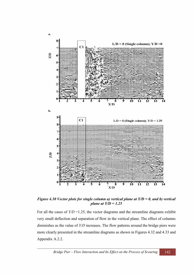
Bridge Pier – Flow Interaction and Its Effect on the Process of Scouring 142
Figure 4.30 Vector plots for single column a) vertical plane at Y/D = 0, and b) vertical plane at Y/D = 1.25
For all the cases of Y/D =1.25, the vector diagrams and the streamline diagrams exhibit
very small deflection and separation of flow in the vertical plane. The effect of columns
diminishes as the value of Y/D increases. The flow patterns around the bridge piers were
more clearly presented in the streamline diagrams as shown in Figures 4.32 and 4.33 and
Appendix A.2.2.
a.
b.
L/D = 0 (Single column); Y/D =0C1
C1

Bridge Pier – Flow Interaction and Its Effect on the Process of Scouring 143
Figure 4.31 Vector plots for two columns cases with L/D = 3 a) vertical plane at Y/D = 0, and b) vertical plane at Y/D = 1.25
a.
b.
C1 C2
C1 C2

Bridge Pier – Flow Interaction and Its Effect on the Process of Scouring 144
Figure 4.32 Streamline plots for single column a) vertical plane at Y/D = 0, and b) vertical plane at Y/D = 1.25
a.
b.
L/D = 0; Y/D =0C1
C1

Bridge Pier – Flow Interaction and Its Effect on the Process of Scouring 145
Figure 4.33 Streamline plots for two columns cases with L/D = 3 a) vertical plane at Y/D = 0, and b) vertical plane at Y/D = 1.25
4.4.2 Time Average Velocity Components Figures 4.34 to 4.41 show the contour plots and profile plots of velocity components in
the vertical plane, in which the streamwise velocity component (u) and the vertical
a.
b.
C1 C2
C1 C2
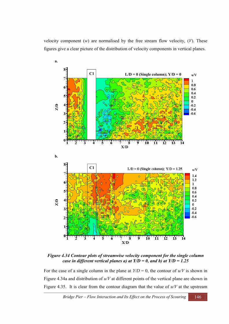
Bridge Pier – Flow Interaction and Its Effect on the Process of Scouring 146
velocity component (w) are normalised by the free stream flow velocity, (V). These
figures give a clear picture of the distribution of velocity components in vertical planes.
Figure 4.34 Contour plots of streamwise velocity component for the single column case in different vertical planes a) at Y/D = 0, and b) at Y/D = 1.25
For the case of a single column in the plane at Y/D = 0, the contour of u/V is shown in
Figure 4.34a and distribution of u/V at different points of the vertical plane are shown in
Figure 4.35. It is clear from the contour diagram that the value of u/V at the upstream
a.
b.
L/D = 0 (Single column); Y/D = 0C1
C1

Bridge Pier – Flow Interaction and Its Effect on the Process of Scouring 147
side of the column is approximately equal to 1 at a distance X/D ≥1.25 measured from
the upstream face of the column. As the flow approaches the column, the value of u/V
becomes smaller and finally reduces to zero at the face of the column. Figure 4.35a shows
that at the upstream side of the column, the values of u/V are decreasing gradually towards
the bed. It was also noticed that u/V for US1 was less than that for US2. This demonstrates
that the u/V diminished gradually as the column was approached. At the downstream side
of the column, it is clear from the contour plot that the value of u/V ranged from -0.6 to 0
at the wake close to the downstream face of the column. The profile plot in Figure 4.35b
for the downstream side of the column shows that the value of u/V ≤ 0 at DS1. The
negative value of u/V indicates the presence of the reverse flow in this region (see Figure
4.34a). The figures exhibit that the value of u/V increases as the flow moves further
downstream and ultimately comes to the normal flow condition. The contour plot of u/V
at the plane Y/D = 1.25 is shown in Figure 4.34b. This figure shows that the maximum
value of u/V occurs at the side of the column, which is approximately equal to 1.2.
Figure 4.35 Profile plots of streamwise velocity component for the single column case in vertical plane at axis of symmetry a) upstream side; b) downstream side
a. b.
-1 0 1 20
1
2
3
4
5
6
7
u/V
Z/D
US1US2
-1 0 1 20
1
2
3
4
5
6
7
u/V
Z/D
DS1DS2DS4

Bridge Pier – Flow Interaction and Its Effect on the Process of Scouring 148
For the case of two in-line columns, contour plots of u/V for L/D = 3 at Y/D = 0 and 1.25
are shown in Figure 4.36. For the rest of the columns arrangements, contour plots are
presented in Appendix A.2.3. Similarly, Figures 4.37 and 4.38a show the velocity profiles
of u/V at different positions of the upstream and downstream sides of the columns for L/D
= 3. Figures in Appendix A.2.5 show the profiles for other arrangements of two columns.
According to the contour plots and the profile plots at the upstream side of Column 1, the
distribution of u/V are almost the same for all the column arrangements. The value of u/V
remains 1 when the flow reaches about 1D distance, measured from the upstream face of
the Column 1; u/V then decreases gradually as the flow moves towards the column. This
type of distribution was also observed in the single column case. However, for the
downstream side of Column 2 and between the two columns, the distribution of u/V varied
with respect to the spacing between the two columns. When L/D = 1, at the downstream
side of Column 2 very close to the column, the minimum u/V was approximately equal
to -0.2, quite similar to the value obtained for the single column case. A gradual increase
in the value of u/V was noticed with increase in the distance from the downstream face
of column 2. This condition applied to all of the arrangements of two in-line columns.
For the spacing L/D ≥ 2, it was observed that the value of u/V < 0.5 was reached within
the zone of around 2D, measured from the downstream face of Column 2.
Considering the flow between two in-line columns, the contour plots and the profile plots,
presented in Appendices A.2.3 and A.2.5 indicate that the value of u/V for the case of
L/D = 2 varies between -0.5 and 0. The negative value of u/V indicates the reverse flow
within the region. Velocity vector diagrams give the evidence of this type of reverse flow.
As the spacing between the two columns increased, the value of the streamwise
component of the flow velocity approaching Column 2 was observed positive. For L/D
> 3, the maximum value of the streamwise component of approach flow for Column 2
was u/V = 0.4. Ataie-Ashtiani and Aslani-Kordkandi (2013) reported that for the case of
L/D = 3, the velocity of flow approaching the downstream column was equal to 0.2-0.3
times the free stream flow velocity, V, which is consistent with the present study results.
On the other hand, the contour plots of the plane at Y/D = 1.25 show that all the
arrangements of columns experience the maximum value of u/V = 1.2 at the side of the
columns. In this plane, for L/D ≤ 3, the maximum value of u/V was at the side of both

Bridge Pier – Flow Interaction and Its Effect on the Process of Scouring 149
columns including the gap between the two columns. However, for L/D ≥ 4, the value of
u/V decreased to approximately equal to 1 as the flow approached the Column 2.
Figure 4.36 Contour plots of streamwise velocity component for the case of two in-line columns with L/D = 3 in different vertical planes a) at Y/D = 0, and b) at Y/D =
1.25
a.
b.
C1 C2
C1 C2

Bridge Pier – Flow Interaction and Its Effect on the Process of Scouring 150
Figure 4.37 Profile plots of streamwise velocity component for two columns case with L/D = 3 in vertical plane at axis of symmetry a) upstream side; b) downstream side
Figure 4.38 Profile plots of velocity components between two columns with L/D = 3 in vertical plane at axis of symmetry a) streamwise component, b) vertical component
The contour plots for the vertical velocity components (w/V) for the single column in the
plane at Y/D = 0 and 1.25 are presented in Figure 4.39 and the distribution profile of w/V
a. b.
0 0.5 1 1.5
0
1
2
3
4
5
6
7
u/V
Z/D
US1US2
-0.5 0 0.5 10
1
2
3
4
5
6
7
u/VZ
/D
DS1DS2DS4
a. b.
-0.5 0 0.50
1
2
3
4
5
6
7
u/V
Z/D
B1
-0.5 0 0.50
1
2
3
4
5
6
7
w/V
Z/D
B1

Bridge Pier – Flow Interaction and Its Effect on the Process of Scouring 151
at different positions of the upstream and downstream sides of the column are presented
in Figure 4.40. At the upstream side of the column, the range of vertical velocity
component (w/V) was from -0.3 to 0.2. The negative value represents the down flow. The
maximum value of this down flow was observed at the upstream side. It is in good
agreement with the experimental values observed by Ahmed (1995). As this down flow
interacts with the boundary layer, a horseshoe vortex was formed at the base just upstream
of a column. As per Dargahi (1989), this is the primary horseshoe vortex. This horseshoe
vortex system interacts with the bed resulting in the more turbulence near the bed.
Distribution of w/V at US1 and US2 of the upstream side of the column is shown in Figure
4.37a. It indicates the generation of high turbulence near the bed, which is evident from
more fluctuation of w/V. At the downstream side of the column, the upward flow region
extending towards the free surface was observed. The maximum value of w/V was found
to be approximately equal to 0.5 at a distance of about 1.5D measured from the
downstream face of the column. Furthermore, it is clear from the figure that the maximum
and minimum value of w/V occurred close to the bed within the wake. Distribution of w/V
in different positions DS1, DS2 and DS4 at the downstream side of the column as shown
in Figure 4.37b shows that the vertical velocity component was heavily fluctuate near the
bed. Significant fluctuation of w/V was observed up to the distance of 4D measured from
the downstream face of a column.
Figure 4.34b shows the contour plot of w/D in the Y/D = 1.25 plane. It shows that down
flow of magnitude 0.2 was observed just upstream from a column and at the side of the
column. The vector diagram in Figure 4.30b and the streamline diagram in Figure 4.31b
give a clear picture of down flow in this region. At the downstream side of this plane, no
significant down flow or up flow was noticed. In the case of the bridge piers with two in-
line columns, Figure 4.41and Appendix A.2.4 show the contour plot of w/V at the planes
Y/D = 0 and 1.25. In these figures for L/D>3, at the immediate upstream side of Column
1, poor quality of distribution of w/V is observed, which could be due to the reflection
during the imaging process. However, at a distance of about 1D measured from the
upstream face of Column 1, the flow is observed as expected. Hence, considering the
flow in this region, at the upstream side of Column 1, the down flow is observed in all
the cases of two in-line columns arrangements. The maximum value of down flow with

Bridge Pier – Flow Interaction and Its Effect on the Process of Scouring 152
w/V was approximately equal to 0.2 observed close to the bed near the column base. This
is also clearly presented in Figure 4.41a. Furthermore, the distribution of w/V at US2,
shown in Figure 4.42a, indicates no down flow throughout the flow depth. In the plane
Y/D = 1.25 as shown in Figure 4.41, down flow with w/V is approximately equal to 0.1,
observed at the upstream and at the side of Column 1. Similar flow is observed at the
upstream side of Column 1 for all the values of L/D.
Figure 4.39 Contour plots of vertical velocity component for single column case in different vertical planes a) at Y/D = 0, and b) at Y/D = 1.25
a.
b.
L/D = 0 (Single column); Y/D =0C1
C1
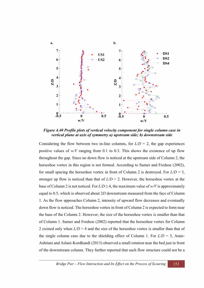
Bridge Pier – Flow Interaction and Its Effect on the Process of Scouring 153
Figure 4.40 Profile plots of vertical velocity component for single column case in vertical plane at axis of symmetry a) upstream side; b) downstream side
Considering the flow between two in-line columns, for L/D = 2, the gap experiences
positive values of w/V ranging from 0.1 to 0.3. This shows the existence of up flow
throughout the gap. Since no down flow is noticed at the upstream side of Column 2, the
horseshoe vortex in this region is not formed. According to Sumer and Fredsoe (2002),
for small spacing the horseshoe vortex in front of Column 2 is destroyed. For L/D = 3,
stronger up flow is noticed than that of L/D = 2. However, the horseshoe vortex at the
base of Column 2 is not noticed. For L/D ≥ 4, the maximum value of w/V is approximately
equal to 0.5, which is observed about 2D downstream measured from the face of Column
1. As the flow approaches Column 2, intensity of upward flow decreases and eventually
down flow is noticed. The horseshoe vortex in front of Column 2 is expected to form near
the base of the Column 2. However, the size of the horseshoe vortex is smaller than that
of Column 1. Sumer and Fredsoe (2002) reported that the horseshoe vortex for Column
2 existed only when L/D > 4 and the size of the horseshoe vortex is smaller than that of
the single column case due to the shielding effect of Column 1. For L/D = 3, Ataie-
Ashtiani and Aslani-Kordkandi (2013) observed a small rotation near the bed just in front
of the downstream column. They further reported that such flow structure could not be a
a. b.
-0.5 0 0.50
1
2
3
4
5
6
7
w/V
Z/D
US1US2
-0.5 0 0.50
1
2
3
4
5
6
7
w/VZ/
D
DS1DS2DS4

Bridge Pier – Flow Interaction and Its Effect on the Process of Scouring 154
horseshoe vortex because of the suppression of down flow due to the formation of the
reattachment regime.
Figure 4.41 Contour plots of vertical velocity component for the two-column case with L/D = 3 in different vertical planes a) at Y/D = 0, and b) at Y/D = 1.25
At the downstream side of Column 2, for all columns arrangements, upward flow exists
with the maximum value of w/V = 0.2, which is about 50% smaller than that of the single
column case and about 30% smaller than the case of Column 1 in the two-column case.
a.
b.
C1 C2
C1 C2

Bridge Pier – Flow Interaction and Its Effect on the Process of Scouring 155
This is due to the sheltering effect of Column 1. According to the contour plots and vector
plots, one can easily see that the flow structures at the wake of Column 2 are totally
different from the single column case. For L/D ≤ 4, a small zone of recirculation was
observed close to the free surface. Similar results were observed by Ataie-Ashtiani and
Aslani-Kordkandi (2013) for L/D = 3. According to the profile plots, the distributions of
w/V at DS1, DS2, and DS4 for L/D ≤ 4 were observed to be similar. However, for L/D >
4 the distribution of w/V at DS1 was observed with a significant negative value close to
the bed. Distribution of w/V at DS2 and DS4 were observed to be similar in all the cases
of two column arrangements.
Figure 4.42 Profile plots of vertical velocity component for the two-column case with L/D = 3 in vertical plane at axis of symmetry a) upstream side; b) downstream side
a. b.
-0.2 0 0.20
1
2
3
4
5
6
7
w/V
Z/D
US1US2
-0.5 0 0.50
1
2
3
4
5
6
7
w/V
Z/D
DS1DS2DS4

Bridge Pier – Flow Interaction and Its Effect on the Process of Scouring 156
Figure 4.43 Profile plots of velocity components between two columns with L/D = 3 in vertical plane at axis of symmetry a) streamwise component, b) vertical component
According to the streamline plots and contour plots of u/V and w/V for two in-line
columns with various spacing, upward and reverse flow are observed between two
columns for L/D =2. Pockets of strong upward and reverse flow occurred close to the bed.
As the spacing increased to L/D = 3, stronger upward flow and reversed flow than in the
case of L/D =2 was identified close to the bed which was observed at the flow separation
zone. As the flow separation for L/D = 3 occurred close to Column 2, strength of flow
(upward and reverse) at downstream side close to Column 1 was higher in the case of
L/D = 2 than that of L/D = 3. When the spacing between two columns increased, the
strength of reverse and upward flow in the wake of Column 1 decreased. As the flow
moves towards Column 2, gradual increase in streamwise velocity and decrease in
vertical velocity component were observed. At the wake of column 2, a very weak
streamwise velocity component of magnitude u/V < 0.2 was noticed for all the cases.
However, the magnitude of upward flow increased with increase in the spacing between
two columns.
4.4.3 Turbulence Intensity Components
The root mean square (rms) values of the components of velocity fluctuations (u′ and w′)
give the turbulence intensity components. In this study, TIu and TIw in the streamwise
a b.
-0.5 0 0.50
1
2
3
4
5
6
7
u/V
Z/D
B1
-0.5 0 0.50
1
2
3
4
5
6
7
w/VZ/
D
B1

Bridge Pier – Flow Interaction and Its Effect on the Process of Scouring 157
direction and the vertical direction, respectively, are normalised using the free stream
velocity, V. The results are presented in contour plots and the distribution profiles at
different positions of upstream, downstream and between the columns (in the case of two
in-line columns).
Figure 4.44 Contour plots of streamwise turbulence intensity component for the single column case in different vertical planes a) at Y/D = 0, and b) at Y/D = 1.25
The contour plots of TIu/V for the single column for the planes Y/D = 0 and 1.25 are
shown in Figure 4.44. Additionally the distribution profiles of TIu/V in the Y/D = 0 plane
a.
b.
TIu/VC1 L/D = 0 (Single column); Y/D = 0
TIu/VC1 L/D = 0 (Single column); Y/D = 1.25
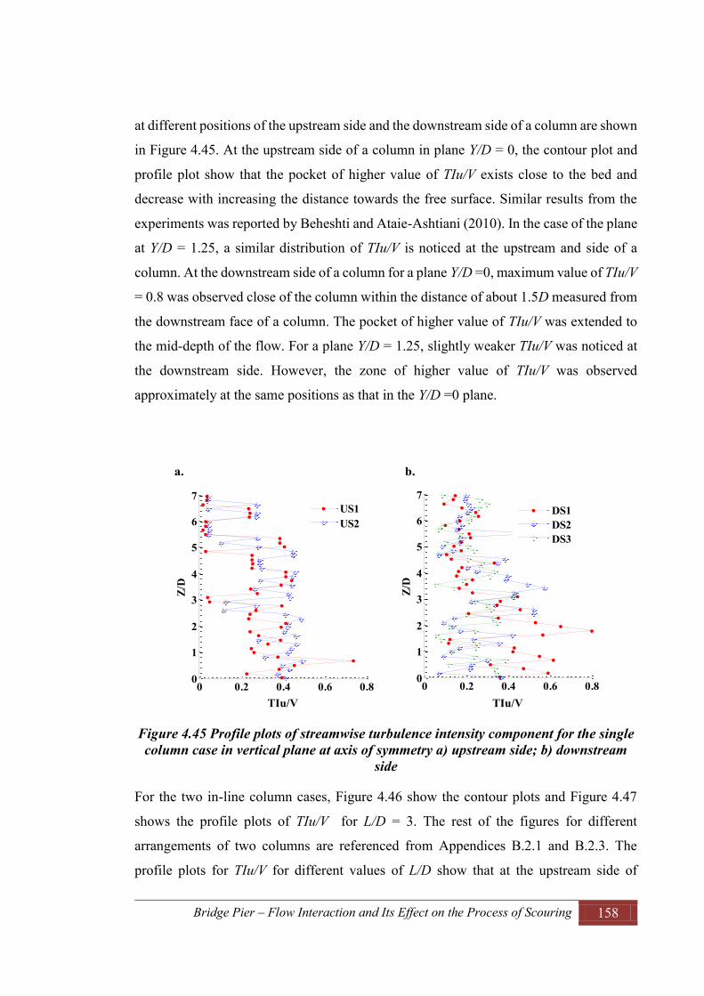
Bridge Pier – Flow Interaction and Its Effect on the Process of Scouring 158
at different positions of the upstream side and the downstream side of a column are shown
in Figure 4.45. At the upstream side of a column in plane Y/D = 0, the contour plot and
profile plot show that the pocket of higher value of TIu/V exists close to the bed and
decrease with increasing the distance towards the free surface. Similar results from the
experiments was reported by Beheshti and Ataie-Ashtiani (2010). In the case of the plane
at Y/D = 1.25, a similar distribution of TIu/V is noticed at the upstream and side of a
column. At the downstream side of a column for a plane Y/D =0, maximum value of TIu/V
= 0.8 was observed close of the column within the distance of about 1.5D measured from
the downstream face of a column. The pocket of higher value of TIu/V was extended to
the mid-depth of the flow. For a plane Y/D = 1.25, slightly weaker TIu/V was noticed at
the downstream side. However, the zone of higher value of TIu/V was observed
approximately at the same positions as that in the Y/D =0 plane.
Figure 4.45 Profile plots of streamwise turbulence intensity component for the single column case in vertical plane at axis of symmetry a) upstream side; b) downstream
side
For the two in-line column cases, Figure 4.46 show the contour plots and Figure 4.47
shows the profile plots of TIu/V for L/D = 3. The rest of the figures for different
arrangements of two columns are referenced from Appendices B.2.1 and B.2.3. The
profile plots for TIu/V for different values of L/D show that at the upstream side of
a. b.
0 0.2 0.4 0.6 0.80
1
2
3
4
5
6
7
TIu/V2
Z/D
US1US2
0 0.2 0.4 0.6 0.80
1
2
3
4
5
6
7
TIu/V2
Z/D
DS1DS2DS3
TIu/V TIu/V

Bridge Pier – Flow Interaction and Its Effect on the Process of Scouring 159
Column 1, the maximum value of TIu/V = 0.5 is observed in the zone close to the bed for
the case of a single column. The same result was reported by Ataie-Ashtiani and Aslani-
Kordkandi (2013). Careful analysis of the flow between two columns for L/D ≤ 4 shows
that the higher values of TIu/V exist close to the bed. It can be noted that the higher value
zone is extended throughout the gaps. For L/D = 6, the maximum value of TIu/V occurs
close to Column 1 at a distance of about 1.5D measured from the face of Column 1. As
the flow approached Column 2, TIu/V was reduced by about 60% of the maximum value,
observed at the downstream side of Column 1.
Figure 4.46 Contour plots of streamwise turbulence intensity component for two columns case with L/D = 3 in different vertical planes a) at Y/D = 0, and b) at Y/D =
1.25
a.
b.
TIu/VC1 L/D = 3; Y/D = 0C2
TIu/VC1 L/D = 3; Y/D = 1.25C2

Bridge Pier – Flow Interaction and Its Effect on the Process of Scouring 160
At the downstream side of Column 2, decrease in the values of TIu/V was noticed, while
comparing the values at the downstream side of Column 1. However, the distribution
profile exhibits a similar pattern as in the upstream side and between two in-line columns.
Furthermore, the figures reveal that the value of TIu/V at the downstream side of Column
2 increases with increase in the spacing between the two columns. Comparison of the
figures for L/D ≤ 3 at the plane Y/D = 1.25 reveals that significant reduction in the value
of TIu/V can be seen at the downstream side of Column 2. However, for L/D ≥ 4, it was
observed that the distribution of TIu/V at the downstream side of Column 2 is similar to
that of the single column case.

Bridge Pier – Flow Interaction and Its Effect on the Process of Scouring 161
Figure 4.47 Profile plots of streamwise turbulence intensitycomponent for two-column case with L/D = 3 in vertical plane at axis of symmetry a) upstream side, b)
downstream side, and c) between two columns
a. b.
c.
0 0.5 10
1
2
3
4
5
6
7
TIu/V
Z/D
US1US2
0 0.5 10
1
2
3
4
5
6
7
TIu/V
Z/D
DS1DS2DS4
0 0.5 10
1
2
3
4
5
6
7
TIu/V
Z/D
B1
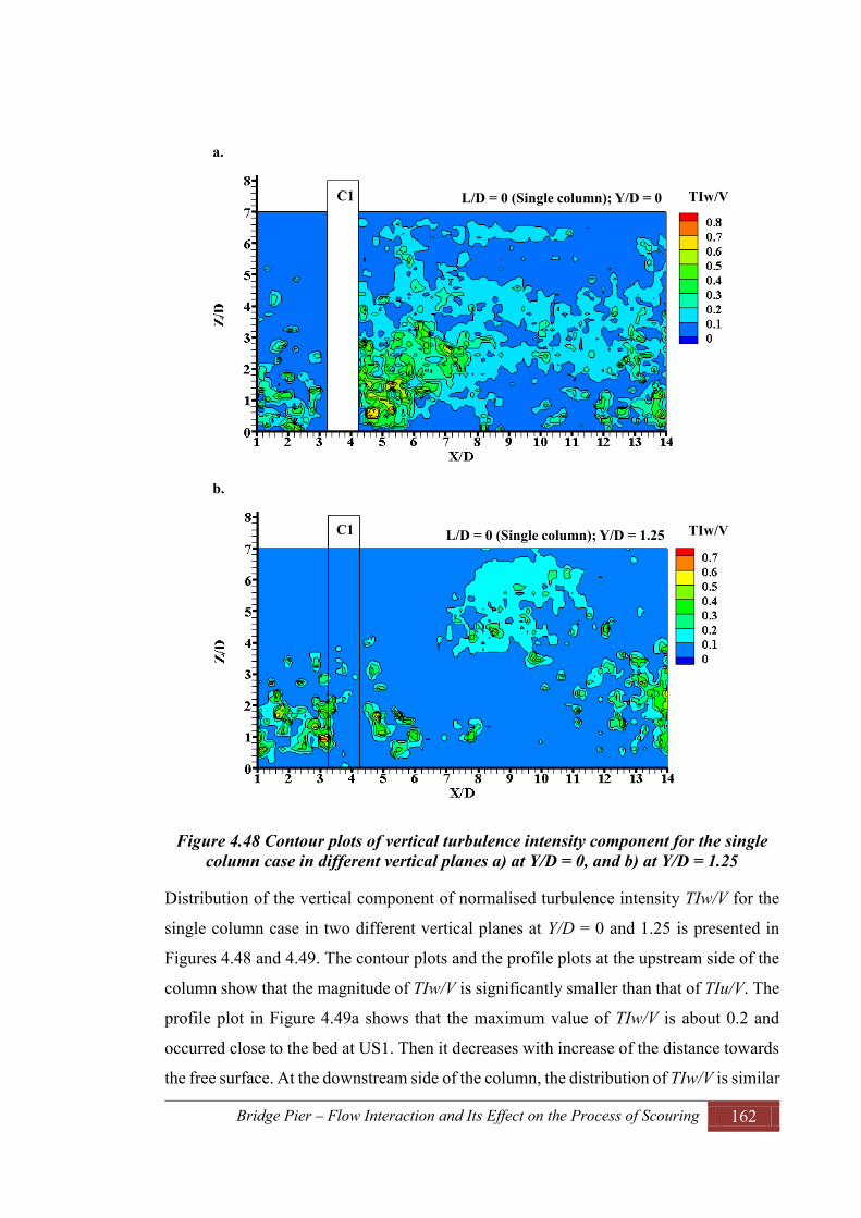
Bridge Pier – Flow Interaction and Its Effect on the Process of Scouring 162
Figure 4.48 Contour plots of vertical turbulence intensity component for the single column case in different vertical planes a) at Y/D = 0, and b) at Y/D = 1.25
Distribution of the vertical component of normalised turbulence intensity TIw/V for the
single column case in two different vertical planes at Y/D = 0 and 1.25 is presented in
Figures 4.48 and 4.49. The contour plots and the profile plots at the upstream side of the
column show that the magnitude of TIw/V is significantly smaller than that of TIu/V. The
profile plot in Figure 4.49a shows that the maximum value of TIw/V is about 0.2 and
occurred close to the bed at US1. Then it decreases with increase of the distance towards
the free surface. At the downstream side of the column, the distribution of TIw/V is similar
a.
b.
TIw/VC1 L/D = 0 (Single column); Y/D = 0
TIw/VC1 L/D = 0 (Single column); Y/D = 1.25

Bridge Pier – Flow Interaction and Its Effect on the Process of Scouring 163
to the distribution of TIu/V with approximately the same value. However, for the contour
plot in the plane Y/D = 1.25, the distribution of TIw/V is different in both magnitude and
order than in the case of TIu/V. From the figure, very weak vertical turbulence intensity
can be noticed in the plane at Y/D = 1.25, except close to the bed.
Figure 4.49 Profile plots of vertical turbulence intensity component for the single column case in vertical plane at axis of symmetry a) upstream side; b) downstream
side
For the case of two in-line columns, the distribution of TIw/V for L/D = 3 is presented in
Figures 4.50 and 4.51. For other values of L/D contour plots and profile plots are
presented in Appendices B.2.2 and B.2.4. According to the figures for all the values of
L/D, approximately the same order and distribution of TIw/V is observed at the upstream
side of Column 1. Similarly, for the plane Y/D = 1.25, the distribution of vertical
turbulence intensity at the upstream side of the Column 1 for all values of L/D is almost
constant.
a. b.
0 0.5 1
0
1
2
3
4
5
6
7
TIw/V
Z/D
US1US2
0 0.5 10
1
2
3
4
5
6
7
TIw/V
TIw
/V
DS1DS2DS4

Bridge Pier – Flow Interaction and Its Effect on the Process of Scouring 164
Figure 4.50 Contour plots of vertical turbulence intensity component for two columns case with L/D = 3 in different vertical planes a) at Y/D = 0, and b) at Y/D = 1.25
a.
b.
TIw/VC1 L/D = 3; Y/D = 0C2
TIw/VC1 L/D = 3; Y/D = 1.25C2
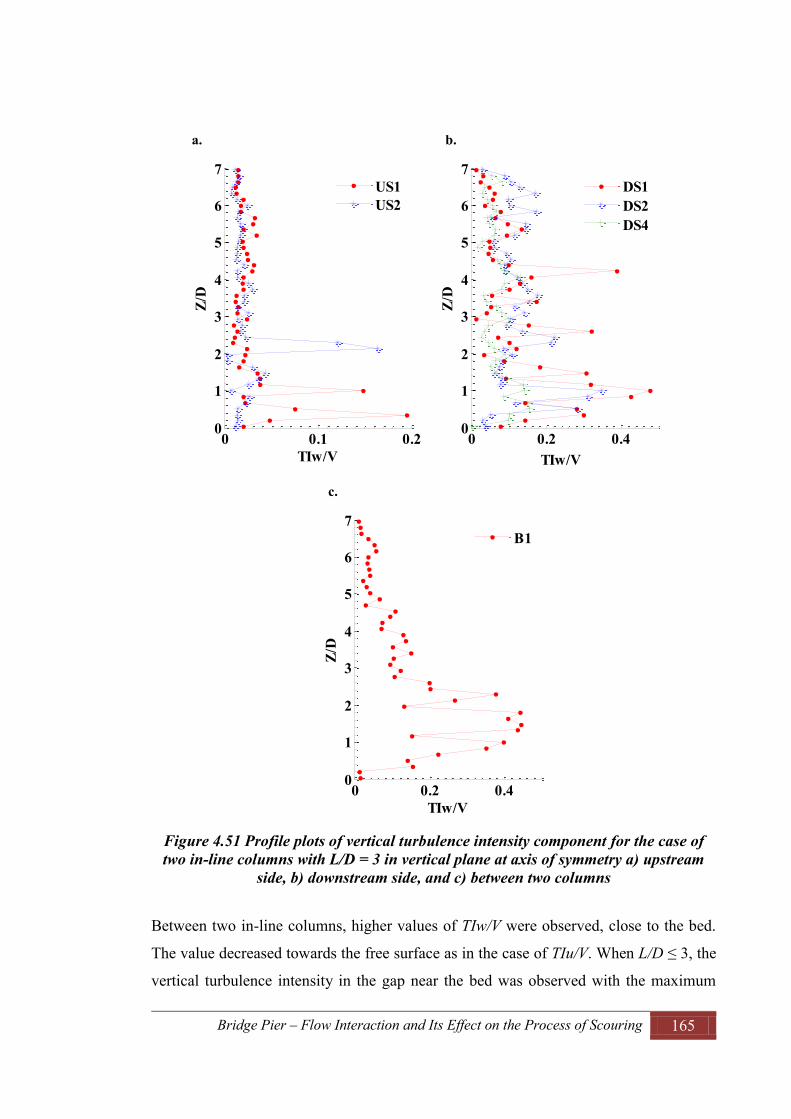
Bridge Pier – Flow Interaction and Its Effect on the Process of Scouring 165
Figure 4.51 Profile plots of vertical turbulence intensity component for the case of two in-line columns with L/D = 3 in vertical plane at axis of symmetry a) upstream
side, b) downstream side, and c) between two columns
Between two in-line columns, higher values of TIw/V were observed, close to the bed.
The value decreased towards the free surface as in the case of TIu/V. When L/D ≤ 3, the
vertical turbulence intensity in the gap near the bed was observed with the maximum
a. b.
c.
0 0.1 0.20
1
2
3
4
5
6
7
TIw/V
Z/D
US1US2
0 0.2 0.40
1
2
3
4
5
6
7
TIw/VZ/
D
DS1DS2DS4
0 0.2 0.40
1
2
3
4
5
6
7
TIw/V
Z/D
B1

Bridge Pier – Flow Interaction and Its Effect on the Process of Scouring 166
value lying in the range of 0.4 to 0.5. While for L/D ≥ 4, the maximum value of TIw/V
was approximately equal to 0.4 close to the Column 1 and gradually decreased as the flow
approached Column 2 and eventually reaches the condition similar to the upstream side
of Column 1. It was noticed that the maximum values of TIu/V and TIw/V between the
two columns for all the values of L/D were approximately the same.
Referring to the profile plots for Y/D =0 plane, shown in Appendix B.2.4, the maximum
value of TIw/V for L/D = 1 at the downstream side of Column 2 was about 50% less than
that of the single column case. The profile plots further revealed that the value of TIw/V
increased as the spacing between the two columns increased. It was also common to
observe that TIw/V gradually decreased in the downstream direction in all the cases of
L/D. For the plane Y/D = 1.25, when L/D ≤ 3, a similar distribution of TIw/V was observed
with a value approximately equal to 0.1. However, for L/D > 3 a slight increase in TIw/V
was noticed at the bank of the downstream side of Column 2, which was further extended
towards the downstream side.
4.4.4 Turbulent Kinetic Energy
The results of turbulent kinetic energy (TKE) in the vertical plane parallel to the flow
direction are presented in this section. It can be noted that the transverse component of
velocity fluctuation has not been considered. Contour plots of TKE/V2 for the single
column case in the vertical planes at Y/D = 0 and 1.25 are presented in Figure 4.52.
Similarly the distribution of TKE/V2 at different positions of the upstream and
downstream side in a plane Y/D=0 is presented in Figure 4. The results from the contour
plots and profile plots indicate that the distribution of TKE/V2 is similar to the distribution
of turbulence intensity. At the upstream side of a column, higher values of turbulent
kinetic energy were observed close to the bed and gradually decreased towards the free
surface. The maximum value of TKE/V2 was approximately equal to 0.3 for both US1 and
US2 at the upstream side of a column. At the downstream side of a column, the maximum
value of TKE/V2 was observed close to the column near the bed. It was about 2 times
greater than that of the upstream side. The profile plot at the downstream side of a column
as shown in Figure 4.53b indicates that the value of turbulence kinetic energy decreases
as the distance increases to further downstream side direction.
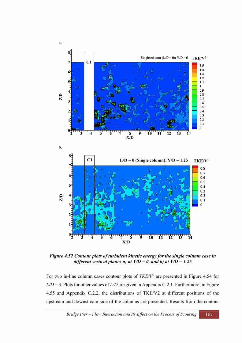
Bridge Pier – Flow Interaction and Its Effect on the Process of Scouring 167
Figure 4.52 Contour plots of turbulent kinetic energy for the single column case in different vertical planes a) at Y/D = 0, and b) at Y/D = 1.25
For two in-line column cases contour plots of TKE/V2 are presented in Figure 4.54 for
L/D = 3. Plots for other values of L/D are given in Appendix C.2.1. Furthermore, in Figure
4.55 and Appendix C.2.2, the distributions of TKE/V2 at different positions of the
upstream and downstream side of the columns are presented. Results from the contour
a.
b.
TKE/V2
C1
TKE/V2C1 L/D = 0 (Single column); Y/D = 1.25

Bridge Pier – Flow Interaction and Its Effect on the Process of Scouring 168
plots and profile plots for various L/D indicate that there is significant change in the
turbulence kinetic energy from upstream to downstream of the columns. At the upstream
side of Column 1, the distributions of TKE/V2 for all the cases of L/D were similar to the
single column case. Between the two columns and at the downstream side of Column 2,
the contour plots show that the distribution of TKE/V2 is more or less similar to that of
the turbulence intensity. The figures exhibit an increase in turbulence kinetic energy
behind the Column 1 as the spacing between the two column increases. For the case of
L/D = 3 and 4, the pocket of higher value of turbulent kinetic energy occurred close to
the Column 2. However, for L/D>4, the value of turbulent kinetic energy decreased as
flow approached Column 2. For example, in the case of L/D = 6, the value of TKE/V2
close to Column 2 at the upstream side was approximately equal to 0.1, about 70% less
than that of the downstream side of Column 1. At the downstream side of Column 2, the
figures indicate that the value of TKE/V2 increases as the spacing between the two
columns increases up to L/D = 3. Further increase in spacing results in the decrease in the
value of TKE/V2.
Figure 4.53 Profile plots of turbulent kinetic energy for the single column case in vertical plane at axis of symmetry a) upstream side; b) downstream side
a. b.
0 0.2 0.40
1
2
3
4
5
6
7
TKE/V2
Z/D
US1US2
0 0.5 10
1
2
3
4
5
6
7
TKE/V2
Z/D
DS1DS2DS4

Bridge Pier – Flow Interaction and Its Effect on the Process of Scouring 169
Figure 4.54 Contour plots of turbulent kinetic energy for the two-column case with L/D = 3 in different vertical planes a) at Y/D = 0, and b) at Y/D = 1.25
a.
b.
TKE/V2C1 L/D = 3; Y/D = 0C2
TKE/V2C1 L/D = 3; Y/D = 1.25C2

Bridge Pier – Flow Interaction and Its Effect on the Process of Scouring 170
Figure 4.55 Profile plots of turbulent kinetic energy for the case of two in-line columns with L/D = 3 in vertical plane at axis of symmetry a) upstream side, b)
downstream side, and c) between two columns
a. b.
c.
0 0.1 0.20
1
2
3
4
5
6
7
TKE/V2
Z/D
US1US2
0 0.2 0.40
1
2
3
4
5
6
7
TKE/V2Z/
D
DS1DS2DS4
0 0.2 0.40
1
2
3
4
5
6
7
TKE/V2
Z/D
B1

Bridge Pier – Flow Interaction and Its Effect on the Process of Scouring 171
4.4.5 Reynolds Shear Stresses
In this study, for the vertical planes parallel to the flow direction, Reynolds shear stresses
are calculated using only the streamwise and vertical components of velocity fluctuation
and are denoted by - . For the presentation of results, - have been normalised
by . Here, represents the mass density of water.
Figure 4.56 Contour plots of Reynolds shear stress for the single column case in different vertical planes a) at Y/D = 0, and b) at Y/D = 1.25
a.
b.
-RS/V2C1 L/D = 0 (Single column); Y/D = 0
-RS/V2C1 L/D = 0 (Single column); Y/D = 1.25
-
-

Bridge Pier – Flow Interaction and Its Effect on the Process of Scouring 172
The contour plots of - on two different longitudinal planes Y/D = 0 and 1.25 for
the single column case is shown in Figure 4.56. Similarly, Figure 4.57 shows the profiles
of - . The contour plots indicate that at the upstream side of a column, -
considerably increases as the flow approaches close to the column. Small pockets of
positive as well as negative values of - were observed near the bed close to the
column. The normalised Reynolds stress values at the upstream side were in the range of
-0.3 < - < 0.2. At the downstream side of a column, a similar trend of distribution
of - was observed with higher values close to the bed. In Y/D = 0 plane, the
pocket of positive and negative values in the range of -0.5 <- < 0.5 was observed
close to the column and extended up to a distance of 3D downstream, measured from the
face of the column. However, in the plane Y/D = 1.25, a positive value of -
approximately equal to 0.3 was observed throughout the depth.
Figure 4.57 Profile plots of Reynolds shear stress for the single column case in vertical plane at axis of symmetry a) upstream side; b) downstream side
a. b.
-0.5 0 0.50
1
2
3
4
5
6
7
RS/V2
Z/D
US1US2
-0.5 0 0.50
1
2
3
4
5
6
7
RS/V2
Z/D
DS1DS2DS4
- -

Bridge Pier – Flow Interaction and Its Effect on the Process of Scouring 173
Figure 4.58 Contour plots of Reynolds shear stress for the case of two in-line columns with L/D = 3 in different vertical planes a) at Y/D = 0, and b) at Y/D = 1.25
a.
b.
-RS/V2C1 L/D = 3; Y/D = 0C2
-RS/V2C1 L/D = 3; Y/D = 1.25C2
-
-
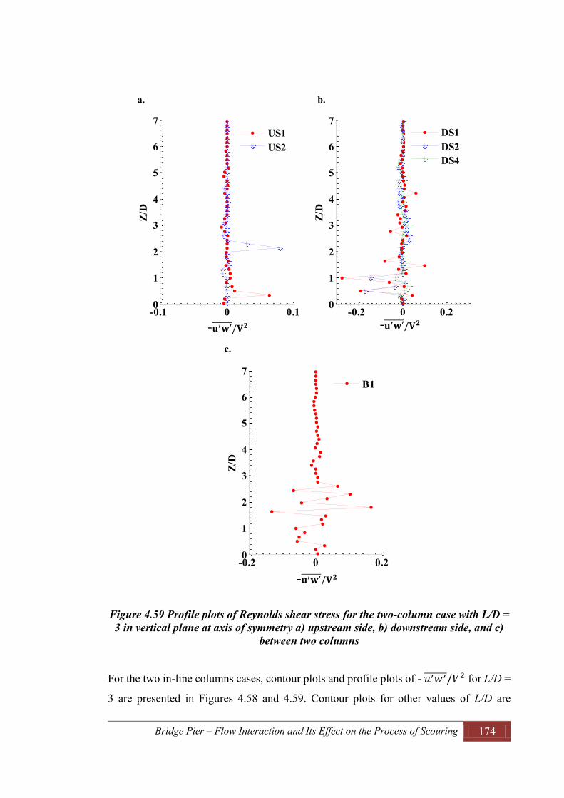
Bridge Pier – Flow Interaction and Its Effect on the Process of Scouring 174
Figure 4.59 Profile plots of Reynolds shear stress for the two-column case with L/D = 3 in vertical plane at axis of symmetry a) upstream side, b) downstream side, and c)
between two columns
For the two in-line columns cases, contour plots and profile plots of - for L/D =
3 are presented in Figures 4.58 and 4.59. Contour plots for other values of L/D are
a. b.
c.
-0.1 0 0.10
1
2
3
4
5
6
7
RS/V2
Z/D
US1US2
-0.2 0 0.20
1
2
3
4
5
6
7
RS/V2Z/
D
DS1DS2DS4
-0.2 0 0.20
1
2
3
4
5
6
7
RS/V2
Z/D
B1
-
-
-
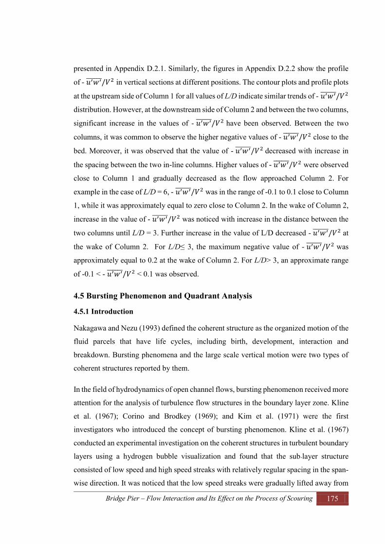
Bridge Pier – Flow Interaction and Its Effect on the Process of Scouring 175
presented in Appendix D.2.1. Similarly, the figures in Appendix D.2.2 show the profile
of - in vertical sections at different positions. The contour plots and profile plots
at the upstream side of Column 1 for all values of L/D indicate similar trends of -
distribution. However, at the downstream side of Column 2 and between the two columns,
significant increase in the values of - have been observed. Between the two
columns, it was common to observe the higher negative values of - close to the
bed. Moreover, it was observed that the value of - decreased with increase in
the spacing between the two in-line columns. Higher values of - were observed
close to Column 1 and gradually decreased as the flow approached Column 2. For
example in the case of L/D = 6, - was in the range of -0.1 to 0.1 close to Column
1, while it was approximately equal to zero close to Column 2. In the wake of Column 2,
increase in the value of - was noticed with increase in the distance between the
two columns until L/D = 3. Further increase in the value of L/D decreased - at
the wake of Column 2. For L/D≤ 3, the maximum negative value of - was
approximately equal to 0.2 at the wake of Column 2. For L/D> 3, an approximate range
of -0.1 < - < 0.1 was observed.
4.5 Bursting Phenomenon and Quadrant Analysis
4.5.1 Introduction
Nakagawa and Nezu (1993) defined the coherent structure as the organized motion of the
fluid parcels that have life cycles, including birth, development, interaction and
breakdown. Bursting phenomena and the large scale vertical motion were two types of
coherent structures reported by them.
In the field of hydrodynamics of open channel flows, bursting phenomenon received more
attention for the analysis of turbulence flow structures in the boundary layer zone. Kline
et al. (1967); Corino and Brodkey (1969); and Kim et al. (1971) were the first
investigators who introduced the concept of bursting phenomenon. Kline et al. (1967)
conducted an experimental investigation on the coherent structures in turbulent boundary
layers using a hydrogen bubble visualization and found that the sub-layer structure
consisted of low speed and high speed streaks with relatively regular spacing in the span-
wise direction. It was noticed that the low speed streaks were gradually lifted away from
Bridge Pier – Flow Interaction and Its Effect on the Process of Scouring 176
the wall and then began to oscillate and finally were ejected from the wall. It was observed
that these processes occurred intermittently and randomly over the surface.
4.5.2 Review on Quadrant Analysis
Corino and Brodkey (1969) investigated the turbulent flow near the solid boundary and
observed the generation and transport processes. It was found that the sub layer was
continuously disturbed by small scale velocity fluctuation and the fluid elements were
periodically ejected outwards from the wall which interacted with the mean flow resulting
in velocity fluctuation. These ejections and resulting fluctuations were believed to be a
factor in the generation of turbulence
Kim et al. (1971) conducted an experimental study on the turbulence structure of a smooth
surface boundary layer in a low speed water flow using hydrogen bubble measurements
and hot wire measurements with dye visualization. They focused on the process of
production of turbulence near the wall. It was discovered that the turbulence energy and
the Reynolds stresses were generated during an intermittent bursting process.
Furthermore, they describe the overall behavior of a flow model during bursting. It was
summarized that the overall model of bursting can be described by three stages of flow
namely: slow lifting of low speed streaks, rapid growth of oscillatory motion, and break
up of oscillation. After completion of these cycles, the velocity profile returns to a form
generally like the mean profile shape.
Many experimental investigations have been conducted on the mechanism of turbulence
production and bursting phenomenon in smooth-wall boundary layers and have produced
an outline of bursting phenomenon which are well accepted at the present time. The
bursting phenomena in smooth boundary layers was described in several comprehensive
reviews by Willmarth (1975); Wallace (1985); Kim (1987); Kline and Afgan (1990); and
Smith et al. (1991). Lu and Willmarth (1973) developed the quadrant technique for the
better understanding of the contribution to Reynolds stresses. According to quadrant
analysis of two dimensional velocity fluctuations u′, and w΄ (or v΄), the bursting process
can be classified in four different classes of events such as: outward interaction (u′>0,
w′>0), ejection (u′<0, w′>0), inward interaction (u′<0, w′<0) and sweep (u′>0, w′<0) in

Bridge Pier – Flow Interaction and Its Effect on the Process of Scouring 177
four different quadrant zones denoted by Q1, Q2, Q3 and Q4 respectively as shown in
Figure 4.60.
Figure 4.60 Definition sketch of four quadrant zones in u-w plane
As reported in Nakagawa and Nezu (1993), the instantaneous Reynolds- stress signal
u′(t)w′(t) is directly related to bursting phenomena. For the generation of turbulence,
ejection and sweep motions are the main events. Hence, sorting functions Ie(t) for ejection
and Is(t) for sweeps are introduced to detect the basic features of the bursting phenomena
and are defined by the following equations:
4.1
4.2
As there are interaction motions contained in ejection and sweep motions, the sorting
functions cannot be used directly to detect the bursting motion. Thus, Lu and Willmarth
)
u′
Outward interactionEjection
Inward interaction Sweep
(u′>0, w′>0) (u′<0, w′>0)
(u′<0, w′<0) (u′>0, w′<0)
Hole
Q1Q2
Q3 Q4

Bridge Pier – Flow Interaction and Its Effect on the Process of Scouring 178
(1973) introduce a threshold level, H (also called the hole size) in u′-w′ quadrant analysis.
They assumed that ejection and sweep motions occur under the following condition:
4.3
where, H is the hole size (0, 1, and 2), are the local root mean square
values of velocity fluctuation in stream-wise and vertical direction respectively
Lu and Willmarth (1973) presented a method to analyse the structure of instantaneous
Reynolds stress, according to which, the Reynolds stresses at a point in the u′-w′ plane
are equal to the sum of contributions measured in four quadrants. The contributions to
Reynolds stresses from four quadrants were computed from the following equation:
4.4
where, is an indicator that detects the production of turbulence.
=1, if and the point (u′, w′) in the u′-w′ plane is in the
ith quadrant; and =0, otherwise.
Shiau (1999) applied the concept of stress fraction, , to analyse the contribution to
Reynolds stress. Stress fraction is defined as the contribution ratio between and
total Reynolds stress at a point in u′-w′ plane, which is given by:
4.5
For hole size H= 0, the sum of fractional contributions from all bursting events is equal
to 1.
Another way of analysing the organization of coherent structure is the probability of
occurrence of bursting events in each quadrant. Keshavarzi and Shirvani (2002) and
Keshavarzi and Gheisi (2006) performed a probability analysis to examine the

Bridge Pier – Flow Interaction and Its Effect on the Process of Scouring 179
organization of coherent structure using the conditional probability analysis. In order to
estimate the probability of occurrence of each event, the following equations have been
proposed:
4.6
4.7
where, is the probability of occurrence of each event, is the number of events in
each class and N is the total number of bursting events.
In recent years, quadrant analysis based on two dimensional velocity information has
been extensively used to analyse the contribution of bursting events for the generation of
turbulence structure. Nakagawa and Nezu (1978); Nakagawa and Nezu (1993); and
Keshavarzy and Ball (1997) investigated two dimensional quadrant analysis of the
bursting process and reported that the sweep and ejection events have higher contribution
for the production of turbulence than outward interaction and inward interaction.
Furthermore, Keshavarzi and Gheisi (2006) proposed a three dimensional quadrant
analysis for the study of the bursting process addressing the effect of transverse velocity
components.
Roussinova et al. (2009) reported the analysis of the instantaneous velocity field
measured by particle image velocimetry (PIV) in a smooth open channel flow using
proper orthogonal decomposition (POD) to expose the vertical structure. The results from
the POD analysis were combined with the results from momentum analysis and
conditional quadrant analysis performed at three different threshold level. It was reported
that the results from quadrant analysis cannot provide useful information about the
extreme events when using the threshold level, H = 0. On the other hand, while using the
larger threshold, i.e. H ≥ 0, there could be significant loss of information about flow
events. However, the quadrant analysis provides the spatial distribution of the important
events such as ejection and sweep. In that study, the effect of flow structure on the mean

Bridge Pier – Flow Interaction and Its Effect on the Process of Scouring 180
flow, the contribution of each event to the Reynolds stress was presented analysing the
profile of stress fractions at each quadrant. It was concluded from this analysis that
ejection and sweep events were the larger contributors to the mean Reynolds stresses.
Furthermore, it was reported that the inward and outward interaction generate about three
times smaller stress fraction than that of ejection and sweep events.
Yang (2010) has theoretically investigated conditionally averaged turbulent structures in
two dimensional uniform flow considering the momentum flux caused by upward and
downward velocity. It was reported that, this momentum flux generated results in
deviation of conditional Reynolds shear stress from expected linear distribution.
Furthermore, the results indicated that the conditional Reynolds stress produced by the
contribution of ejection event is always greater than the classical Reynolds stress, whereas
the Reynolds stress produced by the contribution of sweep event is always less than the
classical Reynolds stress. Additionally, it was reported that the deviation of conditional
turbulence intensities is similar to the deviation of conditional Reynolds stress.
Izadinia et al. (2013) conducted an experimental investigation on the stochastic nature of
instantaneous shear stresses over the scour hole and its influences on sediment
entrainment and transport. It was reported that the probability distribution of
instantaneous Reynolds stresses were distributed in such a way that the tails of the
distribution decayed to zero slower than the Gaussian distribution. On the other hand, the
quadrant analysis indicated that outward and inward interactions were dominant near the
bed at the upstream side of the bridge pier. As the distance from the bed increased,
ejection and sweep events became dominant. The reason behind this was reported as due
to the velocity reversal phenomenon, which occurs near the bed at the upstream side of
the pier. Furthermore, it was indicated that the occurrence probability of sweep events is
more than other events at the upstream side. Dominant sweep events at the upstream side
were reported as the cause of maximum scour depth at this region and transportation of
sediments to the downstream side. The assessment of stress fraction revealed that
contributions of each events to Reynolds stress production are stronger at the downstream
side of the piers.

Bridge Pier – Flow Interaction and Its Effect on the Process of Scouring 181
Keshavarzi et al. (2014) performed three dimensional analysis of turbulent flow structures
around a single circular bridge pier by measuring the instantaneous three dimensional
velocity components using an ADV. In that study, the velocity data were analysed using
the Markov process to investigate the probability of occurrence of bursting events. Three
dimensional octant analysis was used for the better understanding of the bursting events
during sediment entrainment. The concept of conditional transitional probability was
applied for the analysis of coherent turbulent structures. It was concluded from the results
that the external sweep and internal ejection events primarily contribute the sediment
entrainment around a single circular bridge pier.
4.5.3 Results of Quadrant Analysis
In this study, quadrant analysis has been employed to analyse the structure of
instantaneous Reynolds stresses measured around bridge piers consisting of a single
column and two in-line columns. The Reynolds stress at a point is presented as the sum
of contributions measured in four quadrants. The results are analysed based on the
probability of occurrence (Pi) of each quadrant and contribution ratio (stress fraction, Si)
for the production of Reynolds stresses. In this section, the results are analysed for the
flow in u-w plane at the plane of symmetry i.e. Y/D = 0. The results for the single column
and two in-line column cases are presented in this section as given in Figures 4.61 to 4.70
and Appendices E.1 and E.2. In this section, the results associated with the single column
and two columns with L/D = 3 are presented, while the rest of the results are referenced
from figures given in Appendices E.1 and E.2.
The probability of occurrence (Pi) of each of the four quadrants (i = 1, 2, 3 and 4) is
determined from the experimental data using Equations 4.6 and 4.7. Pi, which is plotted
against the normalised depth of flow and the results are shown in Figures 4.61 to 4.65.
For the single column case, Pi at the upstream side (US1) is shown in Figure 4.61.
Referring to this figure, it can be seen that the probability of occurrence of each event
varies with depth of flow. The figure exhibits that the highest value of the depth-averaged
probability of occurrence is in the sweep event (Q4) followed by the outward interaction
(Q1), the inward interaction (Q3) and the ejection events (Q2). This maximum value of
sweep event occurred at the upstream side of a column where the horseshoe vortex and

Bridge Pier – Flow Interaction and Its Effect on the Process of Scouring 182
strong down flow took place. According to Lu and Willmarth (1973), sweep event is
associated with high speed flow that is faster than the average streamwise velocity and
slower than the average vertical velocity. Hence, the excavated bed material from the
upstream side is easily transported to the downstream side. This shows that the bridge
piers experience the maximum scour depth at the upstream side. Furthermore, the
maximum values of Pi close to the bed at Z/D < 2 have been observed in the sweep and
ejection events. Additionally, the results from for the upstream side of the single column
indicate that the value of Pi of ejection event decreases as the distance from the bed
increases towards the free surface.
This trend is consistent with the results presented by Keshavarzy and Ball (1997) and
Izadinia et al. (2013). Probability of occurrence profile of sweep event for the upstream
side of the single column case shows the higher values of Pi throughout the flow depth.
The above results indicate that the sweep event is the most important bursting events for
the entrainment of sediment particles. At the downstream side of the single column case,
profile plots of probability of occurrence of each quadrant are presented in Figure 5.62.
The figure reveals that Pi for ejection event in the wake is observed at a maximum close
to the bed. A similar result is also reported by Izadinia et al. (2013). As discussed in
Section 4.4.1, strong upward flow exists at the wake of the column. Occurrence of a
maximum value of the probability of occurrence of ejection event and strong upward flow
in the wake of a column make the sediments become suspended. However, comparing
the depth average probability of occurrence, the outward interaction was the dominant
event, followed by the ejection, the sweep and the inward interaction events. As reported
by Keshavarzi et al. (2014), outward interaction results in the force vectors being directed
towards the water surface and inward interaction results in the force vectors directed
opposite to the mean flow direction. Hence, outward and inward interactions were not
effective for the entrainment of sediment.

Bridge Pier – Flow Interaction and Its Effect on the Process of Scouring 183
Figure 4.61 Profile plots of probability of occurrence of different quadrants at upstream side (US1) for single column case
Figure 4.62 Profile plots of probability of occurrence of different quadrants at downstream side (DS1) for single column case
Figures 5.63 to 4.65 show the profile plots of the probability of occurrence of each of the
four events for the two in-line columns case with L/D = 3. Considering these figures along
with the figures presented in Appendix E.1, the results indicate that at the upstream side
L/D = 0, Y/D = 0, US1
Q1 Q2 Q3 Q4
0 20 40 60 80 1
0
1
2
3
4
5
6
7
P1
Z/D
0 20 40 60 80 1
0
1
2
3
4
5
6
7
P2
0 20 40 60 80 10
1
2
3
4
5
6
7
P3
0 20 40 60 80 10
1
2
3
4
5
6
7
P4(%) (%) (%) (%)
L/D = 0, Y/D = 0, DS1
Q1 Q2 Q3 Q4
0 20 40 60 80
0
1
2
3
4
5
6
7
P1
Z/D
0 20 40 60 80 10
1
2
3
4
5
6
7
P2
Z/D
0 20 40 60 80 10
1
2
3
4
5
6
7
P30 20 40 60 80
0
1
2
3
4
5
6
7
P4(%) (%) (%) (%)
Bridge Pier – Flow Interaction and Its Effect on the Process of Scouring 184
of Column 1 for all values of L/D, the highest value of Pi occurs in a sweep event as in
the single column case. Comparing the depth average probability of occurrence of a
sweep event for different values of L/D indicates that the value of Pi at the upstream side
of Column 1 increases as the spacing between the two columns increases until L/D = 3.
Further increase in the spacing results in a decrease in the value of Pi of a sweep event.
However, the values of Pi of a sweep event at the upstream side for two column cases
were higher than those for the single column case. As described in Section 4.3.1, in the
two in-line column cases, the shear layer separated from Column 1 was extended more
than that of the single column case to the downstream side. This is the indication of a
larger extension of horseshoe vortex legs towards the downstream side. According to the
simulation results observed by Kirkil et al. (2008), transport of bed sediment is associated
with the motion of the vortical structure detached from the leg of the primary horseshoe
vortex and the sweep event of turbulent burst phenomenon close to the bed. This supports
the fact that the higher scour depth is observed for the two-column case rather than for
the single column. While considering the ejection event at the upstream side of Column
1, it is observed that for L/D = 1, the average value of Pi is similar to the single column
case. For L/D > 1, a significant decrease in the average value of Pi for ejection event was
observed. However, gradual increase in the value of Pi of ejection event was noticed with
increase in the spacing between the two columns. Considering the distribution of Pi in
outward and inward interaction events, for all values of L/D at the upstream side of
Column 1, the average value of Pi in outward interaction was higher than in inward
interaction. Furthermore, it was common to all of the cases that the value of Pi in inward
interaction event increased with increase in the distance from the bed towards the free
surface.
Between two columns, the profile plots for the case of L/D = 2 and 3, only one point was
selected to analyse the probability of occurrence of events. However, for L/D > 4, two
points, one at the downstream side of Column 1 and another point at the upstream side of
Column 2, were selected for analysis. For L/D = 2, the probability of occurrence of
ejection and sweep events (dominant events) were approximately the same. Similar
results were observed in the case of L/D = 3. However, the value of Pi in sweep event
decreased as the spacing increased from L/D = 2 to 3, whereas, the value of Pi in ejection

Bridge Pier – Flow Interaction and Its Effect on the Process of Scouring 185
event increased. For L/D = 2, Pi of outward interaction and inward interaction were
similar. Further increase in the spacing resulted in a decrease in Pi of sweep event. The
probability of occurrence of ejection event at the downstream side of Column 1 increased
until L/D = 3. For L/D > 3, a gradual decrease in the value of Pi was observed. Comparing
these results with the single column case shows that Pi of ejection event remains
approximately the same for the downstream side of a single column and Column 1 of the
two columns cases. However, the value of Pi in sweep event at the downstream side of
Column 1 is higher than that of the single column case. As the flow approaches Column
2 for L/D > 3, a decrease in Pi of sweep event and an increase in ejection event can be
observed.
Figure 4.63 Profile plots of probability of occurrence of different quadrants at upstream side (US1) of Column 1 for the twocolumn case with L/D = 3
At the downstream side of Column 2 in two-column cases, the results reveal that inward
interaction is dominant. Considering ejection and sweep events for all values of L/D,
reveals that the probability of occurrence of ejection event is higher than that of sweep
event. Furthermore, the results indicate that increase in the spacing between two columns
results in decrease in the probability of occurrence of ejection and sweep events. While
comparing the results with the single column case, for L/D = 1, slight increase in Pi of
L/D = 3, Y/D = 0, US1
Q1 Q2 Q3 Q4
0 20 40 60 800
1
2
3
4
5
6
7
P1
Z/D
0 20 40 60 800
1
2
3
4
5
6
7
P20 20 40 60 80
0
1
2
3
4
5
6
7
P30 20 40 60 80
0
1
2
3
4
5
6
7
P4(%) (%) (%) (%)

Bridge Pier – Flow Interaction and Its Effect on the Process of Scouring 186
sweep and ejection events occurred. However, for L/D > 1, the values of Pi in sweep and
ejection events were observed significantly less than those of the single column case.
Figure 4.64 Profile plots of probability of occurrence of different quadrants at downstream side (DS1) of Column 2 for two columns case with L/D = 3
Figure 4.65 Profile plots of probability of occurrence of different quadrants between
two columns (at B1) with L/D = 3
The contribution of each quadrant for production of Reynolds stresses has also been
analysed based on the stress fraction. Contribution of shear stress fractions of four events
(%) (%) (%) (%)
L/D = 3, Y/D = 0, DS1
Q1 Q2 Q3 Q4
0 20 40 60 800
1
2
3
4
5
6
7
P1
Z/D
0 20 40 60 80 10
1
2
3
4
5
6
7
P20 20 40 60 80
0
1
2
3
4
5
6
7
P30 20 40 60 80
0
1
2
3
4
5
6
7
P4
(%) (%) (%) (%)
L/D = 3, Y/D = 0, B1
Q1 Q2 Q3 Q4
0 20 40 60 800
1
2
3
4
5
6
7
P1
Z/D
0 20 40 60 800
1
2
3
4
5
6
7
P20 20 40 60 80
0
1
2
3
4
5
6
7
P30 20 40 60 80
0
1
2
3
4
5
6
7
P4

Bridge Pier – Flow Interaction and Its Effect on the Process of Scouring 187
are presented in Figures 4.66 to 4.70 and Appendix E.2. Figure 4.66 shows the profile
plots of the stress fraction of each event at the upstream side of a single column bridge
pier. The results at the upstream side (US1) of the single column case indicate that the
depth-average stress fraction for sweep events has a higher contribution in the production
of Reynolds stresses than the ejection event. This is because of the existence of down
flow at the upstream side of the column and the result is consistent with the findings by
Yang (2010). He reported that down flow is associated with sweep event. Furthermore,
the figures exhibit that contribution of Si for sweep and ejection events decreases towards
the free surface. At the downstream side of the single column case, Si for ejection event
is observed higher than that of sweep event. This is due to the strong upward flow in the
wake of a column. According to Yang (2010) ejection is associated with upward flow and
produces higher Reynolds stresses than sweep event. Lu and Willmarth (1973) also
reported that about 77% of the contribution to the Reynolds stress is produced by the
ejection event. They further reported that the sweep event also significantly contributes
to the production of Reynolds stress. It was found that the distribution trend and
magnitude of Si for the sweep and ejection events were similar. Additionally, it is clear
from the figures that at the downstream side of the column, Si fluctuates more strongly
than at the upstream side.
For two in-line columns cases, the contribution of Si of each event for the production of
Reynolds stresses at the upstream side of Column 1 are presented in Figure 4.68 and
Appendix E.2. As in the case of the single column, Si of ejection and sweep events close
to the bed at the upstream side of Column 1 are dominant for all values of L/D. However,
at higher depth, outward interaction and inward interaction are associated with higher
values of Si. Similar results were also reported by Izadinia et al. (2013).

Bridge Pier – Flow Interaction and Its Effect on the Process of Scouring 188
Figure 4.66 Profile plots for contribution of stress fraction of different quadrants for the production of Reynolds stress at upstream side of single column
Figure 4.67 Profile plots for contribution of stress fraction of different quadrants for the production of Reynolds stress at downstream side of single column
L/D = 0, Y/D = 0, US1
Q1 Q2 Q3 Q4
-1 -0.5 00
1
2
3
4
5
6
7
S1
Z/D
0 0.5 10
1
2
3
4
5
6
7
S2-1 -0.5 00
1
2
3
4
5
6
7
S30 0.5 1
0
1
2
3
4
5
6
7
S4
L/D = 0, Y/D = 0, DS1
Q1 Q2 Q3 Q4
-1 -0.5 00
1
2
3
4
5
6
7
S1
Z/D
0 0.5 10
1
2
3
4
5
6
7
S2-1 -0.5 00
1
2
3
4
5
6
7
S30 0.5 1
0
1
2
3
4
5
6
7
S4

Bridge Pier – Flow Interaction and Its Effect on the Process of Scouring 189
At the downstream side of Column 1, the value of Si was higher for the ejection event.
Comparing this value with the single column case, the value of Si for the ejection event
at the downstream side of Column 1 was higher for all values of L/D. Furthermore, the
maximum value of Si is observed for L/D = 2. This is due to strong turbulence in the wake
of Column 1, as described in Section 4.4.2. As suggested by Yang (2010), strong
turbulence intensities and hence the maximum Reynolds shear stress are associated with
upward flow, particularly in the wake of a column. Hence, the high values of turbulence
characteristics keep the sediments in suspended form. Gradual decrease in the value of Si
for an ejection event at the downstream side of Column 1 was observed while increasing
the value of L/D. For L/D > 3, at the upstream side of Column 2, outward interaction and
inward interaction became dominant. According to Mianaei and Keshavarzi (2010),
domination of outward interaction and inward interaction is associated with the
deposition of sediment. Hence, the suspended sediments are expected to deposit at the
upstream side of Column 2. However, down flow and horseshoe vortex close the
upstream face of Column 2 keep the sediments entrained. Similar to the downstream side
of Column 1, the maximum value of Si for the ejection event occurred close to the bed at
the downstream side of Column 2. However, considering the depth average value of Si
for the sweep and ejection events at the downstream side of Column 2 indicated a
significant contribution in production of Reynolds stress. As the spacing between two
columns increased, contribution of the ejection and sweep events in the production of
Reynolds stress increased. Comparison revealed that the value of Si of the ejection and
sweep events at the downstream side of Column 2 for all values of L/D was less than that
of Column 1.

Bridge Pier – Flow Interaction and Its Effect on the Process of Scouring 190
Figure 4.68 Profile plots for contribution of stress fraction of different quadrants for the production of Reynolds stress at upstream side of Column 1 for two columns case
with L/D = 3
Figure 4.69 Profile plots for contribution of stress fraction of different quadrants for the production of Reynolds stress at downstream side of Column 2 for two columns
case with L/D = 3
L/D = 3, Y/D = 0, US1
Q1 Q2 Q3 Q4
-1 -0.5 00
1
2
3
4
5
6
7
S1
Z/D
0 0.5 10
1
2
3
4
5
6
7
S2-1 -0.5 00
1
2
3
4
5
6
7
S30 0.5 1
0
1
2
3
4
5
6
7
S4
L/D = 3, Y/D = 0, DS1
Q1 Q2 Q3 Q4
-1 -0.5 00
1
2
3
4
5
6
7
S1
Z/D
0 0.5 10
1
2
3
4
5
6
7
S2-1 -0.5 00
1
2
3
4
5
6
7
S30 0.5 1
0
1
2
3
4
5
6
7
S4

Bridge Pier – Flow Interaction and Its Effect on the Process of Scouring 191
Figure 4.70 Profile plots for contribution of stress fraction of different quadrants for the production of Reynolds stress between two columns with L/D = 3
4.6 Summary
The detailed results from the experimental study of flow structures around bridge piers
comprising a single column and two in-line columns with varying spacing between them
have been presented in this chapter. The measured instantaneous velocity components
were analysed and the results for flow field and turbulence characteristics have been
presented in graphical forms using vector plots, streamline plots, contour plots and profile
plots.
The vector plots and the streamline plots in horizontal planes for the single column case
indicated that the wake of the column experienced reverse flow and recirculation. Close
to the bed, the shear layer, which had separated from the side of the column, converged
at farther distance than that in the upper levels. At the upstream side of the column, there
was a generation of down flow. At the immediate downstream side, reversal and upward
flows were observed. The maximum value of up flow was at a distance of 2D from the
downstream side of column at which the flow was separated. In the two in-line columns
case, for L/D < 2, reverse flow and recirculation was observed only in the wake of Column
2. The share layer separated from Column 1 wrapped around Column 2 and the horseshoe
vortex was formed only in the front of Column 1. When L/D ≥ 3, it was found that the
L/D = 3, Y/D = 0, B1
Q1 Q2 Q3 Q4
-1 -0.5 00
1
2
3
4
5
6
7
S1
Z/D
0 0.5 10
1
2
3
4
5
6
7
S2-1 -0.5 00
1
2
3
4
5
6
7
S30 0.5 1
0
1
2
3
4
5
6
7
S4

Bridge Pier – Flow Interaction and Its Effect on the Process of Scouring 192
flow between the two columns was separated at a distance of 2.5D, measured from the
downstream face of Column 1. Two separate horseshoe vortices were observed in front
of both Column 1 and Column 2, and the rotation of flow occurred behind both columns.
Furthermore, it was noted that the wake behind the single column was larger than that of
the two-column cases.
The results from the contour and profile plots of three dimensional velocity components
in horizontal and vertical planes for the single column case indicated that higher values
of the streamwise velocity component (u/V) occurred at the side of the columns. Negative
values of u/V were observed in the wake of the column, exhibiting the reverse flow in this
region. The maximum transverse velocity component (v/V) was observed at the upstream
side of the column near the zone of shear layer separation. At the upstream side of the
column, a negative value of vertical velocity component (w/V) was observed, indicating
the down flow. Significant fluctuation of w/V occurred up to the distance of 4D measured
from the downstream face of the column. For the two in-line columns case with L/D ≤ 3,
in the gap region, reverse flow was extended throughout the gap between the two
columns. Very small deflection of flow was noticed inside the gap. However, at the
downstream side of Column 2, higher values of v/V were recorded with values
approximately equal to those of the single column case. The contour plots demonstrate
that the strength of reverse flow at the wake of Column 2 increases with an increase in
the value of L/D. Furthermore, it was observed that the magnitude of u/V at the
downstream side of the single column was constantly higher than that of the other cases.
Considering the w/V component of flow for the two-column case with L/D = 2, the gap
experienced positive values of w/V, showing the existence of up flow throughout the gap.
As the spacing between the two columns increased, a stronger up flow occurred compare
to that of L/D = 2. For L/D > 3, a horseshoe vortex in front of Column 2 was formed near
the base of the column. However, the size of the horseshoe vortex was smaller than that
of Column 1, which could be due to the shielding effect of Column 1.
The results on turbulence intensity in three different horizontal planes showed that the
columns experienced very weak turbulence intensity at the upstream side of the columns
with similar behaviour for all cases of column arrangements. The maximum value of
turbulence intensity occurred in the wake of the columns. For all combinations of the

Bridge Pier – Flow Interaction and Its Effect on the Process of Scouring 193
columns, the value of TIu/V was greater than the component TIw/V, whereas the
turbulence intensity in the transverse direction, TIv/V, was much larger than TIu/V and
TIw/V. The value of turbulence components increased with an increase in the spacing
between the two columns. At the downstream side of Column 2, the values of turbulence
intensity components were smaller than the values measured in the single column case
and between two-column cases with different spacing. This could be due to sheltering by
Column1 resulting the reduction in effective approach velocity for Column 2. The
distribution of turbulent kinetic energy (TKE) was similar to the distribution of turbulence
intensities. The maximum value of TKE/V2 took place between the gap, when L/D = 3.
The results indicated that the value of TKE/V2 increased as the spacing between the two
columns increased up to L/D = 3. Further increase in spacing resulted in a decrease in the
value of TKE/V2.
The results on the Reynolds shear stresses in different horizontal planes along the axis of
symmetry indicated that the absolute value of - was higher than that of
and - . The maximum values of Reynolds shear stresses were observed
close to the bed in the wake of the columns. Absolute values of - in the wakes
for both columns in the two-column cases were smaller than those in the case of the single
column. In the wake of Column 2, absolute values of - were observed increasing
with increase in the spacing until L/D = 3. Further increase in spacing resulted in a
decrease in the absolute value of - in the wake of Column 2. The values of -
and - in the wake of Column 2 were approximately the same, about
50% smaller than the values of the single column case. Furthermore, absolute values of -
were higher close to the bed in the wake and decreased to zero towards the free
surface. It was noticed that the value of - decreased with increase in the spacing
between two columns. Higher values of - were observed close to Column 1 and
gradually decreased as the flow approached Column 2.
The quadrant analysis technique was employed to explore the contribution of each
quadrant for the production of Reynolds shear stresses. Analysis was carried out based
on the probability of occurrence and the stress fraction of each quadrant. According to
the probability of occurrence at the upstream side of the single column case, the sweep

Bridge Pier – Flow Interaction and Its Effect on the Process of Scouring 194
event was dominant. Hence, a sweep event was considered as one of the most important
bursting events. The depth average probability of occurrence in the wake of a column
showed that the outward interaction was the dominating event. However, the probability
of occurrence of the ejection event was higher than that of the sweep event. Hence,
sediments in the wake of the column were expected to be in the suspended form. The
results for the two-column cases indicated that at the upstream side of column 1, the
sweep event was dominant. The probability of occurrence of the sweep event increased
with increase in the spacing between the two columns until L/D = 3. Further increase in
the spacing resulted in a decrease in the value of Pi of the sweep event. However, the
values of Pi of the sweep event at the upstream side for two in-line columns cases were
higher than that of the single column case. For L/D > 1, the values of Pi in the sweep and
ejection events behind Column 2 were significantly less than those of Column 1 and the
single column case. The stress fraction analysis indicated that outward and inward
interactions were contributed strongly to the production of Reynolds stresses at the
upstream side of all columns arrangements. For the two in-line column cases, behind
Column 1, the ejection event was dominant and reached the maximum value when L/D =
2. Considering the sweep and ejection events at the downstream side of Column 2,
contribution of Si for the ejection event was higher than that of the sweep event. As the
spacing between the two columns increased, the contribution of the sweep event in the
production of Reynolds stresses increased. Hence, it can be concluded that between and
at the downstream side of the two columns arrangements, there was a significant
contribution of the stress fraction of all quadrants to the production of Reynolds stresses.

Bridge Pier – Flow Interaction and Its Effect on the Process of Scouring 195
CHAPTER 5
RESULTS AND DISCUSSION ON LOCAL SCOUR
5.1 Introduction
5.2 Review on Scour around Bridge Piers
5.3 Temporal Development of Scour Depth
5.4 Equilibrium Scour Depth for Two-Column Case
5.5 Comparison of Observed and Predicted Maximum Scour Depth
5.6 Scour Profile along Line of Symmetry of Bridge Piers
5.7 Width of the Scour Hole
5.8 Summary

Bridge Pier – Flow Interaction and Its Effect on the Process of Scouring 196
5. RESULTS AND DISCUSSION ON LOCAL SCOUR
5.1 Introduction
In this chapter local scour around a bridge pier with a single column and two in-line
circular columns with different spacing are analyzed and presented. Local scour depths
around two in-line circular columns are compared with the scour depth around a single
column. Furthermore, this chapter exhibits the description on the temporal variation of
scour depth, bed profile after scouring and characteristics of scour hole. Additionally, a
semi-empirical equation is developed to capture the effect of spacing between two in-line
circular columns on the scour depth.
5.2 Previous Investigations on Scour around Bridge Piers
In the history of bridge collapse, local scour around bridge piers is found to be one of the
main causes of failure. Local scour around bridge piers has been extensively studied and
numerous scour prediction equations have been developed by several investigators. Most
of the previous studies were based on scour prediction around a single column and the
process has been studied extensively, for example Laursen and Toch (1956); Melville
(1975); Raudkivi and Ettema (1985); Melville and Sutherland (1988); Breusers and
Raudkivi (1991); Yanmaz and Altinbilek (1991); Dey et al. (1995); Melville and Coleman
(2000); Khwairakpam et al. (2012) Radice and Tran (2012). However, in real situations,
employing two or more columns are very common in practice. Only a few investigations
have been made on the group of columns providing little knowledge on scour patterns.
Hannah (1978); Salim and Jones (1998); Richardson and Davis (2001); Sumer et al.
(2005); Ataie-Ashtiani and Beheshti (2006); Mubeen-Beg (2010); Domenech et al.
(2011); and Amini et al. (2012) have conducted various investigations on scour around
bridge piers consisting of multiple columns.
Laursen and Toch (1956) conducted experimental studies on different models of bridge
piers and abutments. The model bridge pier consisted of two shafts joined with a web.
Three-hour long experiments were conducted both in the absence and in presence of webs
at different values of the angle of flow attack. In the case of the pier without a web, it was
concluded that for small angles of approach (0 to 10 degrees) the downstream shaft was

Bridge Pier – Flow Interaction and Its Effect on the Process of Scouring 197
shielded by the upstream shaft resulting in smaller scour depth at the downstream shaft.
Additionally, it was suggested that a separate scour hole for each shaft was formed. On
comparison of scour depth results for circular and rectangular shape piers, it was reported
that the equivalent rectangular pier produced about 15% more scour depth than that of
the circular pier.
Hannah (1978) conducted a series of experimental investigation on scour around single
and multiple columns with tandem and side by side arrangements for different spacing
between the columns. He has conducted seven-hour experiments for the scour depth and
proposed an adjustment factor of 1.25, which was multiplied to seven hours scour depth
to extrapolate the equilibrium scour depth. Furthermore, he conducted two- column
experiments, varying both the spacing and the angle of attack. It was concluded from
those experiments that the equilibrium scour depth first attained at the upstream column
followed by the downstream column. It was reported that when L/D = 1 i.e. two columns
were attached to each other, the scour depth around the two-column system was equal to
the scour depth around the single column case. Furthermore, it was reported that an
increase in spacing between two columns resulted in increase in experience of reinforcing
effect, reaching a maximum at L/D = 2.5 and is evident up to L/D = 11. Reinforcing effect
occurs when the downstream column is placed so that the columns’ scour holes overlap.
This aids in the sediment removal around the upstream column increasing its scour depth.
Additionally he proposed the coefficients to be applied to the single pier scour depth for
the determination of scour depth around two columns.
Nazariha (1996) conducted a series of experimental tests for the study on local scour
around bridge piers consisting of single and two columns. The experimental tests were
conducted for 2 hours duration and clear water flow conditions were applied for all tests.
Additionally an experiment with 90 hours duration was carried out for the study of
temporal variation of the scour depth. It was reported that more than 83% of total scouring
occurred within the first two hours. Hence, equilibrium scour depth was determined using
a factor of 1.4, applied to the observed scour depths after 2 hours duration. For the two-
column cases, the effects of different angle of attack and spacing between two columns
were investigated. According to the experimental results, it was concluded that the greater
the value of angle of attack, the larger were the equivalent diameter of the pier and the

Bridge Pier – Flow Interaction and Its Effect on the Process of Scouring 198
scour depth consequently. On the other hand, from the experiments of two columns with
zero angle of flow attack, it was reported that for the spacing of L/D = 1, the scour depth
was equal to that of the single column case. An increasing trend of scour depth was
reported for the range of 1< L/D ≤ 4. After this, the scour depth was decreased and
ultimately reached the value of scour depth for the single column case. Furthermore it
was reported that a separate scour hole was formed around the two columns when L/D >
5.
Salim and Jones (1998), studied the scour around pile groups and observed that the scour
depth around the pile group decreased as the spacing between the piles increased.
According to Sumer et al. (2005), scour around piles group was caused by the local scour
mechanism around an individual pile and generated by the global scour mechanism over
the entire area of the pile group. They further described the geometrical characteristics of
the scour hole. Ataie-Ashtiani and Beheshti (2006), conducted an experimental
investigation on scour around a group of piles including two piles in tandem arrangement
and concluded that the maximum scour depth around two piles arranged in tandem
arrangement increases with increase in the spacing between the piles. They observed that
the maximum scour depth occurs at the upstream pile when the value of L/D = 3. In the
case of scour depth at the downstream pile, scour depth at this pile is always smaller that
the single pile case. The reason behind this condition was explained by the fact that the
horseshoe vortex at the downstream side pile was smaller than the single pile case and
the existing live bed conditions. Furthermore, it was reported that the scour depth at the
piles with spacing of 3D was 20% more than the scour around a single pier. In this study,
a number of correction factors to predict the maximum local scour depth for the pile group
were developed considering the base equations given by Melville and Coleman (2000)
and Richardson and Davis (2001).
Hager and Unger (2010) investigated the effect of a single–peaked flood wave on pier
scour under clear water scour of a cohesion-less material. In this study, temporal scour
development along with the end scour depth were presented in terms of particle Froude
number based on the maximum approach flow velocity and the mean sediment size. The
results of that study indicated that the end scour depth depended on the peak approach
flow velocity.
Bridge Pier – Flow Interaction and Its Effect on the Process of Scouring 199
Amini et al. (2012) investigated the clear water local scour for a range of submerged and
unsubmerged pile groups (Submerged pile group: the pile groups are capped below the
water surface. Unsubmerged pile group: the plie groups are capped above the water
surface, only pile groups obstruct the flow.) in different configurations and concluded
that the scour depth was dependent on the pier diameter, the pile spacing and the
submergence ratio (the ratio of approach flow depth to the height of pile relative to the
undisturbed streambed). An empirical relationship to predict the local scour depth was
developed, giving the effect of pile group arrangements, pile spacing and submergence
ratio on local scour.
It is clear from the above review that only a few studies have been carried out on scour
around bridge piers consisting of multiple columns and have not provided the correlation
of the flow structure and the scour depth. Reliable equations have not been well developed
for the prediction of scour depth around the bridge piers with multiple columns. Hence,
in this study, detailed investigation on local scour around bridge piers comprising two in-
line circular columns are carried out which is applicable and useful for practicing bridge
engineers. The results of this study quantify the effects of the spacing between two
columns on the maximum scour depth by an appropriate equation. Meanwhile, the results
obtained are correlated with the flow structures around single and two in-line circular
columns. The results can be used to facilitate the position of piers when scouring is a
design concern.
5.3 Temporal Development of Scour Depth The measured data of the experiments as described in Section 3.4.2 are plotted in Figures
5.1 and 5.2. These figures show the temporal development of scour depths around the
upstream column (Column 1) and the downstream column (Column 2) for test duration
up to 75 hours. The temporal development of the scour depth for a single column and two
in-line circular columns with different spacing (1D, 2D and 3D) are monitored and plotted
as shown in Figures 5.1 and 5.2.
Analysing the scour depth results, illustrated in Figure 5.1 revealed that the scour depth
was rapidly developed for the first ten hours of the test duration. Approximately 90% of
the total scour depth was achieved in this duration. The scour depth after 72 hours

Bridge Pier – Flow Interaction and Its Effect on the Process of Scouring 200
duration was about 99% of equilibrium scour depth, calculated using Equations 2.12-
2.14. The rate of scouring continuously reduced with time, and after 72 hours, the
development of scour was very slow. Hence, the maximum duration of the tests was
between 72 and 75 hours.
Figure 5.1 Temporal development of scour depth at Column 1 for a single column
and two columns with L/D = 1, 2 & 3; Time, t = 72-75 hours and V/Vc = 0.74.
0 5 10 15 20 25 30 35 40 45 50 55 60 65 70 75 800
10
20
30
40
50
60
70
80
90
100
110
120
Time (hrs)
Scou
r de
pth
at C
olum
n 1,
ds1
( m
m)
Single ColumnTwo Columns, L/D = 1Two Columns, L/D = 2Two Columns, L/D = 3
Flow
L

Bridge Pier – Flow Interaction and Its Effect on the Process of Scouring 201
Figure 5.2 Temporal development of scour depth at Column 2 for a single column and two columns with L/D = 2 & 3; Time, t = 72-75 hours and V/Vc = 0.74.
In order to determine the equilibrium scour depth, a time factor (Kt) has been applied to
extrapolate the scour depth. The time factor has been calculated using the expressions
developed by Melville and Coleman (2000) as presented in Equations 2.34 – 2.36.
The time factor Kt (72 hours) was calculated as 0.99, i.e. 99% of the equilibrium scour
depth. The present study satisfies the condition of Equation 2.36. Hence, Equations 2.14
and 2.36 have been used to calculate te and Kt (72 hours), respectively and presented in
Table 5.1. In order to compare the present results with the scour depth predicted using
existing equations, a factor (1/Kt) is applied to the scour depth ds, obtained from this study
in 72 hours. The value of scour depth thus obtained is extrapolated equilibrium scour
depths, which are comparable to the predicted scour depth.
0 5 10 15 20 25 30 35 40 45 50 55 60 65 70 75 800
10
20
30
40
50
60
70
80
90
100
110
Time (hrs)
Scou
r de
pth
at C
olum
n 2,
ds2
(mm
)
Single ColumnTwo Columns, L/D = 2Two Columns, L/D = 3
Flow
L
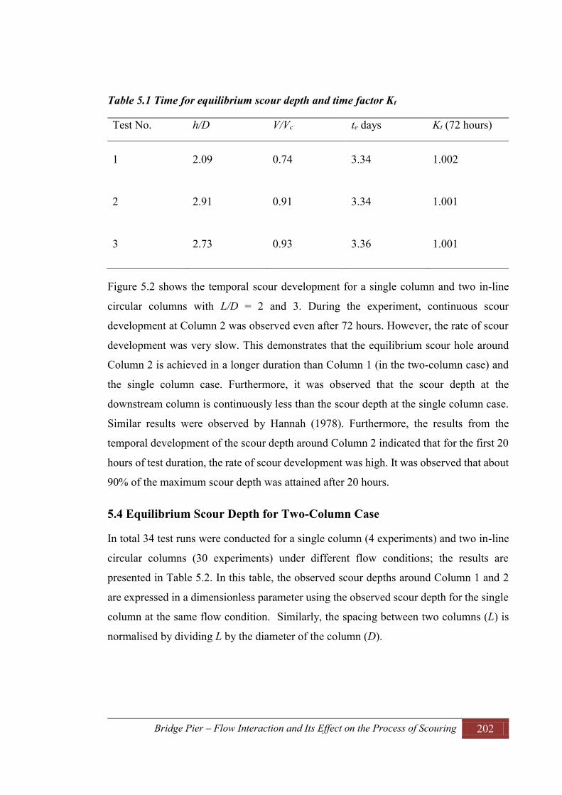
Bridge Pier – Flow Interaction and Its Effect on the Process of Scouring 202
Table 5.1 Time for equilibrium scour depth and time factor Kt
Test No. h/D V/Vc te days Kt (72 hours)
1 2.09 0.74 3.34 1.002
2 2.91 0.91 3.34 1.001
3 2.73 0.93 3.36 1.001
Figure 5.2 shows the temporal scour development for a single column and two in-line
circular columns with L/D = 2 and 3. During the experiment, continuous scour
development at Column 2 was observed even after 72 hours. However, the rate of scour
development was very slow. This demonstrates that the equilibrium scour hole around
Column 2 is achieved in a longer duration than Column 1 (in the two-column case) and
the single column case. Furthermore, it was observed that the scour depth at the
downstream column is continuously less than the scour depth at the single column case.
Similar results were observed by Hannah (1978). Furthermore, the results from the
temporal development of the scour depth around Column 2 indicated that for the first 20
hours of test duration, the rate of scour development was high. It was observed that about
90% of the maximum scour depth was attained after 20 hours.
5.4 Equilibrium Scour Depth for Two-Column Case
In total 34 test runs were conducted for a single column (4 experiments) and two in-line
circular columns (30 experiments) under different flow conditions; the results are
presented in Table 5.2. In this table, the observed scour depths around Column 1 and 2
are expressed in a dimensionless parameter using the observed scour depth for the single
column at the same flow condition. Similarly, the spacing between two columns (L) is
normalised by dividing L by the diameter of the column (D).
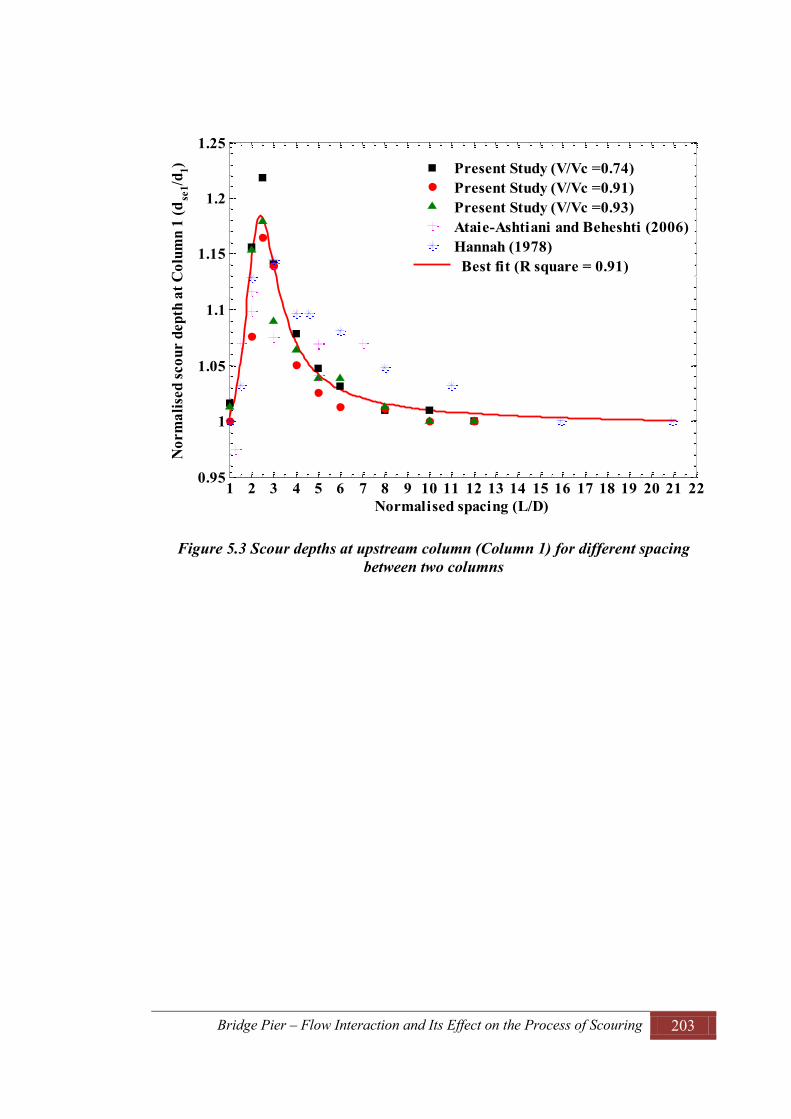
Bridge Pier – Flow Interaction and Its Effect on the Process of Scouring 203
Figure 5.3 Scour depths at upstream column (Column 1) for different spacing between two columns
1 2 3 4 5 6 7 8 9 10 11 12 13 14 15 16 17 18 19 20 21 220.95
1
1.05
1.1
1.15
1.2
1.25
Normalised spacing (L/D)
Nor
mal
ised
scou
r de
pth
at C
olum
n 1
(dse
1/d1)
Present Study (V/Vc =0.74)Present Study (V/Vc =0.91)Present Study (V/Vc =0.93)Ataie-Ashtiani and Beheshti (2006)Hannah (1978) Best fit (R square = 0.91)

Bridge Pier – Flow Interaction and Its Effect on the Process of Scouring 204
Figure 5.4 Scour depths at downstream column (Column 2) for different spacing between two columns
Figure 5.3 displays the data for the scour depth at Column 1 obtained from experiments
of 3 different flow conditions including 34 experimental tests from this study, two sets of
experimental data from Hannah (1978) and Ataie-Ashtiani and Beheshti (2006). In Figure
5.3, the equilibrium scour depth, normalised by the equilibrium scour depth at the
upstream side of the single column (dse1/d1), is plotted against the spacing between two
columns, normalised by the diameter of a column (L/D). Similarly, Figure 5.4 shows the
plots of scour depth data for Column 2 from the present study under different flow
conditions. In this figure, the normalised maximum scour depth at Column 2 (dse2/d1) is
plotted against normalised spacing (L/D).
1 2 3 4 5 6 7 8 9 10 11 12 13 14 15 16 17 18 19 20 21 220.75
0.8
0.85
0.9
0.95
1
Normalised spacing (L/D)
Norm
alise
d sc
our d
epth
at C
olum
n 2
(dse
2/d1)
Present Study (V/Vc = 0.74)Present Study (V/Vc = 0.91)Present Study (V/Vc = 0.93)Hannah (1978)Best fit (R square = 0.88)
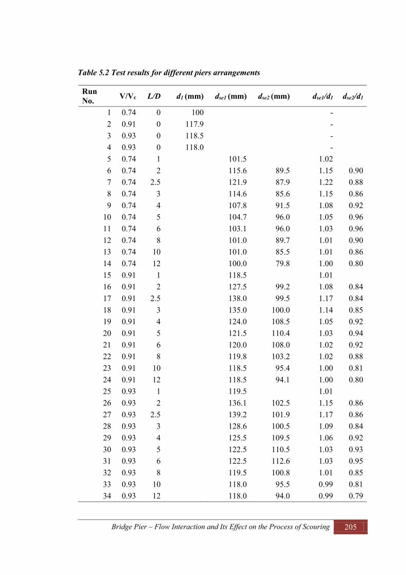
Bridge Pier – Flow Interaction and Its Effect on the Process of Scouring 205
Table 5.2 Test results for different piers arrangements
Run No. V/Vc L/D d1 (mm) dse1 (mm) dse2 (mm) dse1/d1 dse2/d1
1 0.74 0 100 - 2 0.91 0 117.9 - 3 0.93 0 118.5 - 4 0.93 0 118.0 - 5 0.74 1 101.5 1.02 6 0.74 2 115.6 89.5 1.15 0.90 7 0.74 2.5 121.9 87.9 1.22 0.88 8 0.74 3 114.6 85.6 1.15 0.86 9 0.74 4 107.8 91.5 1.08 0.92
10 0.74 5 104.7 96.0 1.05 0.96 11 0.74 6 103.1 96.0 1.03 0.96 12 0.74 8 101.0 89.7 1.01 0.90 13 0.74 10 101.0 85.5 1.01 0.86 14 0.74 12 100.0 79.8 1.00 0.80 15 0.91 1 118.5 1.01 16 0.91 2 127.5 99.2 1.08 0.84 17 0.91 2.5 138.0 99.5 1.17 0.84 18 0.91 3 135.0 100.0 1.14 0.85 19 0.91 4 124.0 108.5 1.05 0.92 20 0.91 5 121.5 110.4 1.03 0.94 21 0.91 6 120.0 108.0 1.02 0.92 22 0.91 8 119.8 103.2 1.02 0.88 23 0.91 10 118.5 95.4 1.00 0.81 24 0.91 12 118.5 94.1 1.00 0.80 25 0.93 1 119.5 1.01 26 0.93 2 136.1 102.5 1.15 0.86 27 0.93 2.5 139.2 101.9 1.17 0.86 28 0.93 3 128.6 100.5 1.09 0.84 29 0.93 4 125.5 109.5 1.06 0.92 30 0.93 5 122.5 110.5 1.03 0.93 31 0.93 6 122.5 112.6 1.03 0.95 32 0.93 8 119.5 100.8 1.01 0.85 33 0.93 10 118.0 95.5 0.99 0.81 34 0.93 12 118.0 94.0 0.99 0.79

Bridge Pier – Flow Interaction and Its Effect on the Process of Scouring 206
For Column 1, an equation (a rational second-degree quadratic equation, Rat22) for the
best-fit line as shown in Figure 5.3 was derived using the nonlinear least square method
with goodness of fit of 0.91 as an R-square value. This relationship is presented in
Equation 5.1. Similarly, an equation for the best-fit line of Column 2 was derived with
goodness of fit of 0.88 as an R-square value and presented in Equation 5.2.
For Column 1
5.1
For Column 2
5.2
where,
a1, a2, a3, a4 and a5, = the model constants for Column 1 obtained experimentally, which
are presented in Table 5.3.
b1, b2, b3, b4 and b5, = the model constants for Column 2 obtained experimentally, which
are presented in Table 5.3.
dse1 = the maximum scour depth at upstream side of Column 1 in the case of two in-line
circular columns
dse2 = the maximum scour depth at upstream side of Column 2 in the case of two in-line
circular columns
d1 = the equilibrium scour depth at upstream side of the pier in the case of single
column
s = the normalised spacing between two columns = L/D
L = the centre to centre distance between two columns

Bridge Pier – Flow Interaction and Its Effect on the Process of Scouring 207
D = the diameter of a column
Table 5.3 Model constants
Column 1 Column 2 Model Constant Value Model Constant Value
0.995 0.780
-4.165 -9.155
5.249 34.010
-4.286 -11.650
5.360 41.510
The right hand sides of Equations 5.1 and 5.2 are expressions of column-spacing factor
between two columns. Thus the equations can simply be expressed as:
For Column 1
5.3
For Column 2
5.4
where, Ks1 and Ks2 are the column-spacing factors for Columns 1 and 2, respectively,
considering the effect of spacing between two columns, which are functions of s (=L/D).
Referring to Figure 5.3, the best-fit line shows the maximum scour depth at Column 1
occurs when the spacing between columns was 2.5D, which was about 18% higher than
the value obtained for the single column. It can be noted that, in actual practice the
maximum scour might occur at the spacing between 2D and 3D. When the spacing
between columns was 1D, i.e. two columns touching each other, the scour depth was
observed to be approximately the same as the scour depth for the single column case. The

Bridge Pier – Flow Interaction and Its Effect on the Process of Scouring 208
scour depth increased as the spacing between the columns increased up to 2.5D, and then
started to decrease with an increase in the spacing between the columns of the bridge pier.
According to Hannah (1978), the reason behind this could be due to the reinforcing effect
of Column 2. He further reported that, for the spacing around 2.5D, the Column 1
experienced the maximum reinforcing effect and this effect existed until the spacing
between the two columns was less than or equal to 10D. In the present study, the
experiments were conducted for the spacing up to 12D. It was observed that the scour
depth at Column 1 for spacing more than 10D was nearly equal to the scour depth for the
single column case. According to Sumer and Fredsoe (2002), the increase in the scour
depth around Column 1 can partly be due to the increase in horseshoe vortex flow. It was
reported that for L/D < 3, the presence of the downstream column caused blockage of
flow, resulting in an increase in the size of lee-wake vortices. Hence, a larger horseshoe
vortex, formed in front of Column 1, can cause a larger scour depth.
Recalling the results on the flow structures around bridge piers from Chapter 4, it was
observed that for L/D < 3, vortex shedding occurred only behind Column 2. Hence, the
flow pattern was more or less similar to the single column case. However, the turbulence
characteristics such as turbulence intensity, turbulent kinetic energy and Reynolds shear
stresses were notably different from the single column case. When the spacing was in the
range of 2 ≤ L/D ≤ 3, stronger turbulence structures were noticed behind Column 1.
Generally, more sediments are expected to remain in suspended form, which can easily
be washed to the downstream side. Hence, a higher scour depth can be expected at
Column 1. Moreover, the results from bursting analysis indicates that the probability of
occurrence (Pi) of a sweep event at the upstream side of Column 1 increases as the
spacing between two columns increases up to L/D = 3. Further increase in the spacing
results in decrease in the value of Pi of a sweep event. In addition to this, the values of Pi
of a sweep event at the upstream side for two in-line columns cases were observed higher
than that of the single column case. This result strongly supports the fact that for the two
in-line circular column case, the maximum scour depth can be observed at the upstream
side of Column 1, when L/D is approximately equal to 2.5. This shows that the maximum
scour depth results obtained in the present study are consistent with the results on flow
structures as summarised above.

Bridge Pier – Flow Interaction and Its Effect on the Process of Scouring 209
Figure 5.4 shows the effect of spacing between two in-line circular columns on the
maximum scour depth around Column 2. Comparing the results, as indicated in Figures
5.3 and 5.4, clearly illustrates that the scour depth at Column 2 is constantly smaller than
the single column case. This is due to the destruction of the horseshoe vortex in front of
Column 2. The results on flow structures in Chapter 5 indicated that for L/D < 3, only one
horseshoe vortex was formed. Two separate horseshoe vortices were generated only when
L/D > 3. On the other hand, reduction in the velocity approaching Column 2 decreases
the effect of horseshoe vortex at Column 2 due to sheltering by Column 1. In addition to
this, the results from the bursting analysis indicated that the probability of occurrence of
sweep and ejection events at the upstream side of Column 2 were significantly less than
that of the single column case. Hence, the above results clearly show a sound correlation
between the results on flow structures and scour around Column 2. Furthermore, the
results on scour depths indicated that at spacing of L/D = 2.5, the scour depth observed at
Column 2 was about 75% of the maximum scour depth at Column 1. Additionally, Figure
5.4 indicates that the maximum value of scour depth at Column 2 can be spotted when 5
< L/D < 6.
5.5 Comparison of Observed and Predicted Maximum Scour Depths
Based on the single column scour depth, Equation 5.3 can be used to predict the maximum
scour depth around bridge piers consisting of two in-line circular columns. In this study,
different existing equations to predict the maximum scour depth for a single pier as
presented in Section 2.3.8 were used to calculate the scour depths for a single column,
which is multiplied by column-spacing factors Ks1 and Ks2 to predict the corresponding
scour depths for two in-line columns cases. However, for the case of predicted scour
depth from this study, the observed scour depths around a single column from different
sets of experiments were taken and multiplied by column-spacing factors to calculate the
predicted scour depths for two in-line columns cases.

Bridge Pier – Flow Interaction and Its Effect on the Process of Scouring 210
Figure 5.5 Comparison of predicted and observed scour depths for two-column bridge piers
For the comparison of the predicted and the observed scour depths, Equations 2.37, 2.38,
2.44 and 2.48 given by Laursen and Toch (1956), Melville and Coleman (2000), Ameson
et al. (2012) and Sheppard et al. (2014), respectively were used to calculate the scour
depth around single column and modified by multiplying by the column-spacing factors,
Ks1 and Ks2. The predicted scour depths were calculated using the above-mentioned
modified equations and the results were compared with the observed scour depths. Figure
5.5 shows the comparison of the predicted and observed maximum scour depths at
Column 1. The figure shows that the predicted scour depths using the equation given by
Laursen and Toch (1956) consistently under-predict the scour depths. However, the
prediction falls within the ±20% error lines. Similarly, the predicted scour depths using
the equation proposed by Ameson et al. (2012) also under-predict the results, falling
outside the ±20% error lines. Results of the experimental study conducted by Ferraro et
al. (2013) also show that the HEC-18 methodology, developed by Ameson et al. (2012),
under-predicts when estimating the maximum scour depth around bridge piers. On the
other hand, Figure 5.5 exhibits that the scour depths predicted, based on the equations
40 50 60 70 80 90 100 110 120 130 140 150 16040
50
60
70
80
90
100
110
120
130
140
150
160
Observed scour depth, mm
Pred
icte
d sc
our
dept
h, m
m
dse, from this study
dse, using Ameson et al. (2012) for d1
dse, using Laursen and Toch (1956) for d1
dse, using Melville and Coleman (2000) for d1
dse, using Sheppard et al. (2014) for d1
Flow
L
± 20% error line
1:1 line

Bridge Pier – Flow Interaction and Its Effect on the Process of Scouring 211
developed by Melville and Coleman (2000) and Sheppard et al. (2014), are consistently
over the experimental results. However, the prediction using the equation by Sheppard et
al. (2014) is closer to the line of perfect agreement, which is less than 12% over
prediction. Hence, it is clear from the above the comparison suggests that the equation by
Sheppard et al. (2014) can be considered the most appropriate equation that can be used
for reasonable prediction of the maximum scour depth at bridge piers comprising two in-
line circular columns.
5.6 Scour Profile along Centerline of the Bridge Piers
Hannah (1978) conducted an experimental study of the bed profile after scouring at the
downstream side of the bridge pier. He found that aggraded materials flattened with time.
The zone of influence of bridge piers was extended approximately to 3D upstream of the
front column and 25D behind the downstream column and reached the maximum width
of 10D across the flume at the downstream end of the aggradation zone. Additionally it
was reported that the shape of the zone of influence around the bridge pier was similar in
both single column and two-column cases.
Figure 5.6 Length scale of scour profile (Ahmed (1995)
Ahmed (1995) reported that most of the models of scour developments observed by
earlier investigators are primarily based on the similarity of the scour profile. Ahmed
(1995) conducted a series of laboratory experiments to study the behaviour of length scale
of scour profile as defined in Figure 5.6. He reported that at the upstream side of the
bridge pier, the average slope of the scour hole was observed about 35o, which is
approximately equal to the angle of repose of bed materials. Furthermore, the upstream
extent of the scour hole was reported larger for the finer bed material and smaller for the
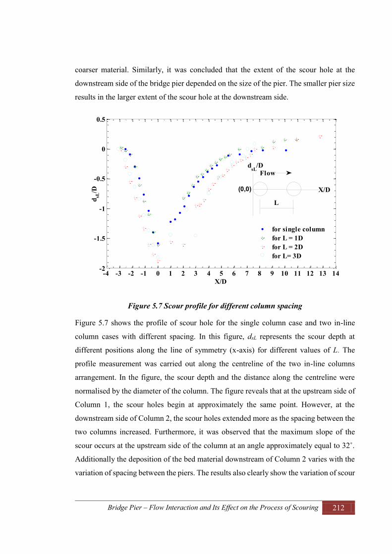
Bridge Pier – Flow Interaction and Its Effect on the Process of Scouring 212
coarser material. Similarly, it was concluded that the extent of the scour hole at the
downstream side of the bridge pier depended on the size of the pier. The smaller pier size
results in the larger extent of the scour hole at the downstream side.
Figure 5.7 Scour profile for different column spacing
Figure 5.7 shows the profile of scour hole for the single column case and two in-line
column cases with different spacing. In this figure, dsL represents the scour depth at
different positions along the line of symmetry (x-axis) for different values of L. The
profile measurement was carried out along the centreline of the two in-line columns
arrangement. In the figure, the scour depth and the distance along the centreline were
normalised by the diameter of the column. The figure reveals that at the upstream side of
Column 1, the scour holes begin at approximately the same point. However, at the
downstream side of Column 2, the scour holes extended more as the spacing between the
two columns increased. Furthermore, it was observed that the maximum slope of the
scour occurs at the upstream side of the column at an angle approximately equal to 32˚.
Additionally the deposition of the bed material downstream of Column 2 varies with the
variation of spacing between the piers. The results also clearly show the variation of scour
-4 -3 -2 -1 0 1 2 3 4 5 6 7 8 9 10 11 12 13 14-2
-1.5
-1
-0.5
0
0.5
X/D
d sL/D
for single columnfor L = 1Dfor L = 2Dfor L= 3D
Flow
L
(0,0) X/D
dsL
/D

Bridge Pier – Flow Interaction and Its Effect on the Process of Scouring 213
depth with respect to the spacing between columns, which was described in detail in
Section 5.4.
5.7 Width of the Scour Hole
Hannah (1978) observed in his experiments that the width of the scour hole remains
constant with a value of approximately 9D, while the length of influence zone changed
linearly until two independent holes are formed. It was reported that two independent
scour holes were established at L/D = 8 after 2 hours and L/D = 10 after 7 hours.
Richardson and Abed (1993) reported that the knowledge of the top width of the scour
hole at piers is important to design the scour countermeasures (for example extent of rip
rap needed as a scour countermeasure) and to design the spacing of bridge piers to ensure
there is not any overlapping of the scour holes. According to the authors, the top width
of the scour holes at piers is a function of the depth of the scour hole and the angle of
repose of bed material in water. The equation for predicting the width of the scour hole
is given as:
= 5.5
where,
= the top width of the scour hole measured from each side of column
= the maximum scour depth
K = the bottom width of the scour hole related to the depth of scour
θ = the angle of repose of the bed material ranging from 30o to 44o
If the bottom width of the scour hole is equal to the scour depth ( ), the value of K is
equal to 1. Hence the top width of the scour hole in cohesion-less material would vary
from 2.07 to 2.8 . On the other hand, for K=0, the top width of the scour hole would
vary from 1.07 to 1.8 . Hence the top width of the scour hole ranges from 1.07 to 2.8
.
In the present study, the maximum widths of scour hole were measured for the different
values of L/D between two in-line columns of bridge piers. Figure 5.8 shows the plot of

Bridge Pier – Flow Interaction and Its Effect on the Process of Scouring 214
the normalised width of the scour hole (ws/D) against the spacing between the piers (L/D).
The variation of the width of the scour hole for different spacing between columns under
different flow condition was clearly presented in this figure. In the figure width of scour
hole was denoted by wsL, where L = 0, 1, 2, 3… It is clear from the figure that the width
of the scour hole varies from 6D to 9D. The width of scour hole for the single column
was less than that for the two in-line columns cases. However for L/D = 1, ws was
observed to be almost equal to the single column case. For L/D ≤ 3, ws was observed
increasing with increase in the spacing between the two columns. For the range 3 < L/D
< 5, very small fluctuation of ws was noticed. Furthermore, the figure reveals that when
the value of L/D is around 3, the maximum value of ws can be around 9D. When L/D >
5, significant decrease in ws was noticed. For L/D ≥ 10, it was observed that two separate
scour holes were developed around each column. Additionally, it was observed that the
width across the midpoint between the two piers was larger than the widths across the
piers.
Figure 5.8 Variation of width of the scour hole for different spacing between two columns
-1 0 1 2 3 4 5 6 7 8 9 10 115
5.5
6
6.5
7
7.5
8
8.5
9
9.5
10
L/D
wsL
/D
for V/Vc = 0.91
for V/Vc = 0.93
for V/Vc = 0.710.74
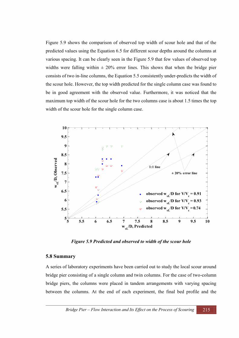
Bridge Pier – Flow Interaction and Its Effect on the Process of Scouring 215
Figure 5.9 shows the comparison of observed top width of scour hole and that of the
predicted values using the Equation 6.5 for different scour depths around the columns at
various spacing. It can be clearly seen in the Figure 5.9 that few values of observed top
widths were falling within ± 20% error lines. This shows that when the bridge pier
consists of two in-line columns, the Equation 5.5 consistently under-predicts the width of
the scour hole. However, the top width predicted for the single column case was found to
be in good agreement with the observed value. Furthermore, it was noticed that the
maximum top width of the scour hole for the two columns case is about 1.5 times the top
width of the scour hole for the single column case.
Figure 5.9 Predicted and observed to width of the scour hole
5.8 Summary
A series of laboratory experiments have been carried out to study the local scour around
bridge pier consisting of a single column and twin columns. For the case of two-column
bridge piers, the columns were placed in tandem arrangements with varying spacing
between the columns. At the end of each experiment, the final bed profile and the
5 5.5 6 6.5 7 7.5 8 8.5 9 9.5 105
5.5
6
6.5
7
7.5
8
8.5
9
9.5
10
wsL
/D, Predicted
wsL
/D, O
bser
ved
observed wsL
/D for V/Vc = 0.91
observed wsL
/D for V/Vc = 0.93
observed wsL
/D for V/Vc = 0.71
± 20% error line
1:1 line
0.74
Bridge Pier – Flow Interaction and Its Effect on the Process of Scouring 216
geometry of the scour holes were measured and the results were presented in tabular as
well as in graphical forms.
Experiments on temporal development of scour depths around bridge piers were
conducted for a period of 72 or 75 hours. The experiments were carried out for a single
and two column bridge piers with spacing 1D, 2D and 3D. The scour depths at different
elapsed time were monitored and recorded for further analysis. It was observed that
approximately 90% of the total scour depth was achieved within the first 10 hours of the
experiments. After 72 hours, the equilibrium scour depth was achieved at the upstream
column. For the downstream column, continuous scour development was observed even
after 72 hours. This shows that the equilibrium scour depth at the downstream column is
attained in a longer duration than that for the upstream column (two in-line circular
columns) as well as for the single column case.
Overall 34 experiments were carried out for the local scour measurement around bridge
piers. Using these local scour depth data along with the maximum scour depth data from
the past investigations, the equations for the best fit line for Columns 1 and 2 have been
derived using the nonlinear least square method with a goodness of fit of 0.91 and 0.88
as an R-square values which were given by Equations 5.1 and 5.2, respectively. From
Equations 5.3 and 5.4, column-spacing factors, Ks1 and Ks2, were proposed that could be
used with the existing scour depth equations to predict the maximum scour depth for two
in-line column cases. Furthermore, it was observed from the experiments that the
maximum scour depth occurred at Column 1 when the spacing between the two columns
was 2.5D. The maximum observed value of local scour depth for the two in-line circular
columns was around 18% higher than the value obtained for the single column case. The
reasons for maximum scour depth at the spacing of 2.5D were found to be associated with
the reinforcing effect of Column 2, the strong horseshoe vortex at Column 1, strong
turbulence characteristics at the wake of Column 1, and the highest probability of
occurrence of sweep events at the upstream side of Column 1.
Furthermore, the final bed profiles were measured, and the results were presented in
Figure 5.5. It is clear from the figure that at the upstream side of the columns, the scour
holes begin approximately at the same point. However, at the downstream side, the scour

Bridge Pier – Flow Interaction and Its Effect on the Process of Scouring 217
hole was extended more as the spacing between the two columns increased. Additionally,
the slope of the scour hole was found to be approximately 32˚. Another important
geometric parameter of the scour hole, the width of the scour hole, was measured for each
experiment. It was observed that the width of the scour hole varied from 6D to 9D. When
the spacing between the two columns was about 3D then the maximum value of the width
of the scour hole was observed, which was equal to 9D. Furthermore, it was noticed that
the maximum top width of the scour hole for the two-column case was about 1.5 times
the top width of the scour hole for the single column case.

Bridge Pier – Flow Interaction and Its Effect on the Process of Scouring 218
CHAPTER 6
CONCLUSION AND RECOMMENDATIONS
6.1 Introduction
6.2 Conclusions
6.3 Recommendations for Future Research

Bridge Pier – Flow Interaction and Its Effect on the Process of Scouring 219
6. CONCLUSION AND RECOMMENDATIONS
6.1 Introduction
In the history of bridge failure, scour around the bridge piers has been reported as the
main cause of failure. More than 60% of bridge failures are associated with the scour and
other hydraulic reasons. The effect of bridge failure is directly reflected in the social and
economic development of a nation. The main reason behind the bridge failure due to
scour is poor design of pier foundations. Many investigations have been made attempting
to estimate the maximum scour depth and to understand the mechanism of scour around
bridge piers. Most of the previous investigations were based on the scour and the flow
structure around a single pier. This is reflected in the wide range of equations developed
by several investigators for the estimation of local scour depth around bridge piers. There
are limited studies on scour around the bridge piers comprising a group of columns.
Additionally, the flow around the bridge piers comprising two or more in-line columns is
not well investigated. However, in practice, bridge piers often consist of multiple columns
in tandem arrangement to support the loading of the structure. Thus a detailed study on
scour and flow around bridge piers with two in-line circular columns has been
experimentally carried out. This study has presented the efforts made for advanced
understanding of research and practice on flow structures and the scour depth around
bridge piers by addressing the challenges related to the aforementioned problems.
6.2 Conclusions
The main contribution of this research is the detailed study on the flow structure
interaction and quantifying the maximum local scour depth around bridge piers consisting
of one circular column or two in-line circular columns. In this study, the effects of spacing
between the two columns on the flow structure and the scour depth around bridge piers
have been thoroughly investigated. The work consisted of the design of the physical
model and experimental tests for the study of flow structures and scour around bridge
piers. A series of experimental tests were conducted using a single column and two
cylindrical columns with circular cross sections. The tests comprised of measuring
instantaneous three dimensional velocity components, experimental investigation of
temporal variation of the scour depth around a single column and two-column bridge
Bridge Pier – Flow Interaction and Its Effect on the Process of Scouring 220
piers, and analysis of the equilibrium scour depth under various conditions of column
arrangements. An acoustic Doppler velocimetry (ADV) and particle image velocimetry
(PIV) techniques were employed to measure the instantaneous three dimensional velocity
components. To measure the scour depth and the final bed profile, a Vernier depth gauge
with a least count of 0.1 mm was used. Similarly, to measure the flow rate, an
electromagnetic flow meter with an accuracy of ± 0.4% was used.
Two flumes with different sizes were employed for the experimental tests, including
Flume 1 (19 m long, 0.61 m wide and 0.61 m deep) and Flume 2 (6 m long, 0.25 m wide
and 0.25 m deep). Flume 1 was used for the study of flow structures in different horizontal
planes using ADV. This flume was also used for the experimental tests on scouring
profiles. The other flume with a smaller size (Flume 2) was used for investigating flow
structures in vertical planes using the PIV technique. Both flumes were equipped with an
electromagnetic flow meter, regulating the gate and the pump. Based on the width of the
flume, the diameter of model column was selected in such a way that there was no
contraction effect on the depth of scour. The diameters of the adopted model columns
were 55 mm and 16 mm for Flume 1 and Flume 2, respectively. The flume width to the
column diameter ratios was checked, ensuring they were greater than 10. Uniformly
graded non-cohesive sand of mean grain size (d50) of 0.85 mm was used as a bed material.
The size of the bed material was determined in such a way that there was no grain size
effect on the scour depth. All tests were conducted under the clear water condition with
different values of critical velocity ratios (V/Vc = 0.38, 0.74, 0.91, 0.93 and 0.96). For
each flow condition, different tests were carried out including a single column and two
in-line circular columns with different spacing between them (L/D = 0 to 12). Altogether
28 tests of fixed bed experiments were carried out for the study of flow structures.
Additionally, 34 moveable bed experiments were conducted for the study of the scour
depth.
The measured instantaneous velocity components were analysed and the results for flow
field and turbulence characteristics were presented in graphical forms using vector plots,
streamline plots, contour plots and profile plots. The results from the vector plots and
streamline plots for single column case indicated that there is a generation of down flow
due to the pressure gradient induced at the upstream face of column. At the immediate

Bridge Pier – Flow Interaction and Its Effect on the Process of Scouring 221
downstream side, reversal, rotational as well as upward flows were observed. For the two-
column cases, the maximum value of up flow was observed at a distance of 2D from the
downstream side of the column at which the flow was found to be separated. For L/D <
2, reverse flow and recirculation was observed only in the wake of Column 2. The flow
regime in this situation is called “extended body regime”. When L/D = 3, the shear layer
separated from Column 1 re-attached on the upstream side of Column 2, which is known
as “re-attachment regime”. This regime is principally characterised by formation and
shedding of eddies in the gap between two columns. Further increase in spacing resulted
in the formation of vortex shedding at the downstream side of both Column 1 and Column
2. Hence, it is called “co-shedding regime”. Comparison of the flow behind the single
column and the two in-line columns reveals that the wake behind the single column case
was larger than that of the two-column cases.
The results from the contour and profile plots of three dimensional velocity components
in horizontal and vertical planes indicated that higher and lower values of streamwise
velocity component (u/V) were observed at the side and in the wake of a column,
respectively. Higher values of negative transverse velocity component (v/V) were
observed at the upstream side near the zone of shear layer separation. At the downstream
side positive values of v/V were observed i.e. the flow converged in the wake of the
column. Negative values of vertical velocity components (w/V) observed at the upstream
face of the column, and indicated the presence of down flow. As this down flow interacted
with the boundary layer, a horseshoe vortex was formed at the base just upstream of the
column. At the downstream side of the column, significant fluctuation of w/V was
observed up to the distance of 4D measured from the downstream face of the column. For
the two-column cases, when L/D ≤ 3, the reverse flow was extended throughout the gap.
Furthermore, the results revealed that the strength of reverse flow at the wake of Column
2 increased with increase in the value of L/D. For L/D = 2, no down flow was noticed at
the upstream side of Column 2. Hence, the horseshoe vortex in this region was not
formed. As the spacing between two columns increased, stronger up flow was observed.
For L/D > 3, the horseshoe vortex in the front of Column 2 was formed near the base of
Column 2. However, the size of the horseshoe vortex at the upstream side of Column 2
was smaller than that of Column 1, which could be due to shielding effect of Column 1.

Bridge Pier – Flow Interaction and Its Effect on the Process of Scouring 222
The three dimensional turbulence intensity components of the flow around the bridge
piers were determined by calculating the root mean square value of velocity fluctuations.
The results indicated that weak turbulence intensity occurred at the upstream side of
bridge piers. However, the maximum values of turbulence intensity were observed in the
wake of the columns. Furthermore, it was noticed that the turbulence intensity in the
transverse direction was much larger than that of streamwise and vertical directions. For
two-column cases, the values of turbulence intensity components were found to increase
with increase in the spacing between two columns. Additionally, the results revealed that
the magnitudes of turbulence intensity in the wake of Column 2 are smaller than in the
single column case and in the gap of the two-column cases. This is due to the sheltering
effect of Column 1 that resulted in the reduction of flow velocity approaching Column 2.
Furthermore, the turbulent kinetic energy of the flow was determined by taking the mean
of the turbulence normal stresses. The results indicated that the distribution of turbulent
kinetic energy was similar to the distribution pattern of turbulence intensities. It was
common to all the cases that higher values of turbulence kinetic energy were observed
close to the bed and gradually decreased towards the free surface. The results from the
two-column cases with L/D = 3 showed that the maximum value of turbulence kinetic
energy occurred between the gap. However, the values of turbulent kinetic energy in the
wake of Column 2 increased as the spacing between the two columns increased up to L/D
= 3. Further increase in spacing resulted in a decrease in the value of turbulence kinetic
energy.
Using the three dimensional data of velocity fluctuations, normalised Reynolds stresses
on three different planes (u-v, u-w and v-w planes) were calculated as - , -
and - . Based on analysing the Reynolds stresses in horizontal planes
along the axis of symmetry, it was observed that the absolute value of - was
constantly higher than that of - and - . For all the cases, maximum
values of Reynolds stresses were observed close to the bed. Furthermore, it was observed
that the absolute value of - in the wake for the two-column cases were smaller
than that in the case of the single column. According to the results obtained in vertical
planes, the absolute values of - were higher close to the bed in the wake and
decreased to zero towards the free surface. Comparing the results for the two-column

Bridge Pier – Flow Interaction and Its Effect on the Process of Scouring 223
cases, it was found that the value of - decreased with increase in the spacing
between the two columns. Higher values of - were observed in the wake of
Column 1 and gradually decreased as the flow approached Column 2.
In order to analyse the structure of instantaneous Reynolds stresses measured around the
bridge piers, the quadrant analysis based on the probability of occurrence (Pi) of each
quadrant and the contribution ratio (stress fraction, Si) for the production of Reynolds
stresses were employed. The results indicated that at the upstream side of the single
column, based on the probability of occurrence, sweep event was dominant. Higher
values of sweep and ejection events occurred close to the bed and gradually decreased
towards the free surface. In the single column case, at the downstream side, outward
interaction was the dominant event, followed by ejection, sweep and inward interaction
events. Considering the results for ejection and sweep events, higher values of Pi occurred
in the ejection event. Hence, the sediments were expected to remain in the suspended
form at the downstream side of the column. For the two in-line columns cases, at the
upstream side of Column 1, Pi increased as the spacing between the two columns
increased until L/D = 3. Further increase in the spacing resulted in a decrease in the value
of Pi of sweep event. However, the values of Pi of sweep event at the upstream side for
two-column cases were observed higher than that of the single column case. This is the
reason, which supports higher scour depth for the two-column case rather than the single
column. Behind Column 2, for all values of L/D, probability of ejection event was
observed higher than sweep event. For the two columns cases, both ejection and sweep
events around Column 2 were observed significantly less than that of the single column
case. The results support the fact that the scour depth around Column 2 is less than that
of Column 1 and the single column case. On the other hand, the results on stress fraction
indicated that outward interaction and inward interaction contributed strongly in the
production of Reynolds stress at the upstream side of all of the two-column arrangements.
For the two-column cases, behind Column 1, the ejection event was dominant and reached
the maximum value when L/D = 2. However, at Column 2, outward interaction and
inward interaction were dominant. Comparing the results for all events, it was found that
the stress fraction of all quadrants contributed significantly to the production of the
Reynolds stress.

Bridge Pier – Flow Interaction and Its Effect on the Process of Scouring 224
A series of experimental tests for the study of the local scour profile around bridge piers
was carried out under different flow conditions. Four tests including a single column, and
two in-line columns with spacing 1D, 2D and 3D were conducted for studying the
temporal development of local scour depths. The results revealed that approximately 90%
of the total scour depth at Column 1 was achieved within the first 10 hours of the
experiments. After 72 hours, the equilibrium scour depth was achieved at the upstream
column. For Column 2, around 90% of the maximum scour depth was achieved after 20
hours. Furthermore, it was observed that the maximum scour depth at Column 2 was
continuously smaller than that of the single column case. In addition, altogether 34
experiments were carried out under different flow conditions for the study of local scour
around bridge piers. The results indicated that the maximum scour depth occurred at
Column 1 when the spacing between two columns was 2.5D. The maximum value of local
scour depth for the two-column case was about 18% higher than the value obtained for
the single column case. Furthermore, an equation for the best-fit line was derived using
the nonlinear least square method, given by Equations 5.1 and 5.3. Similarly, an equation
of the best-fit line for Column 2 is given by Equations 5.2 and 5.4. The coefficients of
spacing between columns, Ks1 and Ks2were proposed for Column1 and Column2,
respectively that could be used with the existing scour-depth prediction equations to
calculate the maximum scour depth for two in-line column cases. Additionally, the results
from final bed profiles indicated that at the upstream side of Column 1, the scour holes
began approximately at the same point. However, at the downstream side of Column 2,
the scour hole was extended more as the spacing between two columns increased. The
width of the scour hole was measured for all experiments and it was observed that the
width of the scour hole varied from 6D to 9D. The maximum width of the scour hole for
the two-column cases was observed at a spacing of 3D, which was approximately 1.5
times more than the width of the scour hole for the single column case.
In summary, it is clearly demonstrated that the flow structures around the two in-line
cylindrical columns of bridge piers is more complex than that of the single column case.
Furthermore, the spacing between two columns significantly affect the flow structures
particularly in the wake of the columns. The results indicated that, for L/D < 3, vortex
shedding occurred only behind Column 2. Hence, the flow pattern is more or less similar
Bridge Pier – Flow Interaction and Its Effect on the Process of Scouring 225
to the single column case. However, the turbulence characteristics such as turbulence
intensity, turbulent kinetic energy and Reynolds shear stresses are notably different from
for the single column. When the spacing is in the range of 2 ≤ L/D ≤ 3, stronger turbulence
structures were noticed behind Column 1. More sediments are expected to remain in
suspended form, which can easily be washed to the downstream side. Hence, a higher
scour depth can be expected at Column 1. Moreover, the results from the local scour tests
exhibit that the maximum scour depth occurred at Column 1 when the spacing between
two columns is L/D = 2.5. The above results of flow structures and local scour are highly
correlated. Hence, it can be concluded that for tandem arrangements of two in-line
cylindrical columns, the spacing in the range of 2 < L/D < 3 is the most critical at which
the columns experience the highest turbulence and hence the maximum scour depth.
6.3 Recommendations of Future Research
The main aim of this research was to study the flow structure interaction in the process
of scouring around bridge piers consisting of two in-line circular columns. To meet the
main objective of this research, the present study acted as a fundamental investigation.
Notwithstanding the fact that the present study confirmed a notable progress in
understanding the flow structure around two cylindrical columns, thorough investigation
on this topic is still not complete. Based on the findings of this study, the following
recommendations are made for further understanding and clarification of the flow
structures and scour around bridge piers with two in-line cylindrical columns:
1. In the present study, all the experiments on flow structures were conducted under
flatbed conditions with a steady flow situation. However, effects of scour on flow
structures have not been investigated. Although the present results give very good
information on the flow structures before commencement of scour, an additional
set of experiments are required to be conducted under moveable bed conditions to
study the effect of scour hole on flow structures.
2. Experiments in the present study were conducted using only cylindrical columns
with circular cross-sections. However, in real situations many different shapes
exist. Hence, experiments with different shapes of columns can be carried out for
better understanding of the shape effect. In addition, experiments with varied

Bridge Pier – Flow Interaction and Its Effect on the Process of Scouring 226
width of column would be useful. Effect of dune and anti-dune, water depth and
vegetation are other conditions arise in real situation, which is recommended for
the future research.
3. For deep understanding of vortex shedding events, which are the main contributor
to the turbulent kinetic energy, PIV measurements on the horizontal planes would
be useful. By conducting these measurements, the relationship between the
shedding events in the upstream side and in the wake could be investigated.
4. A single set of uniform sediment as the bed material was used in this study, which
is an ideal condition in the lab. However, non-uniform sediment has more
practical significance. Therefore, for future research, it is recommended that non-
uniform sediments be used for more accurate and practical results.
5. In this study, all the experiments on scouring were conducted under clear water
condition. In reality, bridge sites experience different types of flow conditions
especially during floods or rainy seasons; scouring often happens under live bed
conditions. Hence, a well-designed physical model is recommended to investigate
the scour characteristics under live bed conditions.
6. Angle of attack is another important parameter and needs to be considered during
the experiments. In the present study, only zero angle of attack was employed.
However, the variation of the angle of attack is strongly recommended to be taken
into account for future research to investigate its interference effects on the
horseshoe vortex system.
7. Although the experimental investigations can provide comparatively more precise
and accurate results, they are costly and more time consuming. From the economic
point of view, research on bridge scouring based on the finite element numerical
modelling using verified software packages is highly recommended for future
research in this area. Nonetheless selected field results or laboratory tests are
required to validate the numerical outputs.

Bridge Pier – Flow Interaction and Its Effect on the Process of Scouring 227
REFERENCES
2005. Bridge Scour Manual. Florida Department of Transportation.
A KESHAVARZI & A SHIRVANI. 2002. Probability analysis of instantaneous shear
stress and entraind particles from the bed. Proceedings of the CSCE/EWRI of
ASCE Environmental engineering conference, Niagara.
A KESHAVARZY & JE BALL 1997. An analysis of the characteristics of rough bed
turbulent shear stresses in an open channel. Stochastic Hydrology and Hydraulics,
11, 193-210.
A. KUMAR & U. KOTHYARI 2012b. Three-Dimensional Flow Characteristics within
the Scour Hole around Circular Uniform and Compound Piers. Journal of
Hydraulic Engineering, 138, 420-429.
A. MELIH YANMAZ & H. DOGAN ALTINBILEK 1991. Study of Time-Depenbent
Local Scour around Bridge Piers. Journal of Hydraulic Engineering, 117, 1247-
1268.
A. QADAR. 1981. The Vortex Scour Mechanism at Bridge Piers ICE Proceedings.
Thomas Telford, 71, 3.
A.A. BEHESHTI & B. ATAIE-ASHTIANI 2010. Experimental study of Three-
Dimensional Flow Field around a Complex Bridge Pier. Journal of Engineering
Mechanics, ASCE, 136, 143-154.
ALESSIO RADICE & CHAU K TRAN 2012. Study of sediment motion in scour hole of
a circular pier. Journal of Hydraulic Research, 50, 44-51.
ALI REZA KESHAVARZI & ALI REZA GHEISI 2006. Stochastic nature of three
dimensional bursting events and sediment entrainment in vortex chamber.
Stochastic Environmental Research and Risk Assessment, 21, 75-87.
ALIREZA KESHAVARZI, BRUCE MELVILLE & JAMES BALL 2014. Three-
dimensional analysis of coherent turbulent flow structure around a single circular
bridge pier. Environmental Fluid Mechanics, 1-27.

Bridge Pier – Flow Interaction and Its Effect on the Process of Scouring 228
ANDRES DOMENECH, F.J. VALLES MORAN, G. PALAU SALVADOR & HANS
BIHS. 2011. Experimental and numerical modelling of scour at bridge piers 10th
Hydraulic Conference, Brisbane, Australia. Engineers Australia.
ARVED J RAUDKIVI & ROBERT ETTEMA 1983. Clear-water scour at cylindrical
piers. Journal of Hydraulic Engineering, 109, 338-350.
ARVED J. RAUDKIVI & ROBERT ETTEMA 1985. Scour at Cylindrical Bridge Piers
in Armored Beds. Journal of Hydraulic Engineering, 111, 713-731.
ARVED J. RAUDKIVI 1998. Loose Boundary Hydraulics, Rotterdam, Netherlands/
Brookfield, USA, A.A. Balkema.
ASHISH KUMAR & UMESH C. KOTHYARI 2012a. Three-Dimensional Flow
Characteristics within the Scour Hole around Circular Uniform and Compound
Peirs. Journal of Hydraulic Engineering, 138, 420-429.
ATA AMINI, BRUCE W. MELVILLE, THAMER M. ALI & ABDUL H. GHAZALI
2012. Clearwater Local Scour around Pile Groups in Shallow-Water Flow.
Journal of Hydraulic Engineering, 138, 177-185.
B. ATAIE-ASHTIANI & A. A. BEHESHTI 2006. Experimental Investigation of Clear-
Water Local Scour at Pile Groups. Journal of Hydraulic Engineering, 132, 1100-
1104.
B. DARGAHI 1989. The Turbulent flow field around a circular cylinder. Experiments in
fluids, 8, 1-12.
B. M. SUMER, K. BUNDGAARD & J. FREDSOE. 2005. Global and Local Scour at
Pile groups Fifteenth International Offshore and Polar Engineering Conference,
Seoul, Korea.
B. MUTLU SUMER & JØRGEN FREDSØE 1997. Hydrodynamics around cylindrical
structures, Advance Series on Ocean Engineering, 12, World Scientific.
B. MUTLU SUMER & JORGEN FREDSOE 2002. The Mechanics of Scour in the
Marine Environment, Advance Series on Ocean Engineering, Toh Tuck Link,
Singapore, World Scientific Publishing Co. Pte. Ltd.
Bridge Pier – Flow Interaction and Its Effect on the Process of Scouring 229
B. W. MELVILLE & A. J. SUTHERLAND 1988. Design Method for Local Scour at
Bridge Piers. Journal of Hydraulic Engineering, 114, 1210-1226.
B. W. MELVILLE 1992. Local Scour at Bridge Abutments. Journal of Hydraulic
Engineering, 118, 615-631.
B.M. SUMER, N. CHRISTIANSEN & J. FREDSOE 1997. The horseshoe vortex and
vortex shedding around vertical wall-mounted cylinder exposed to waves. Journal
of Fluid Mechanics, 332, 41-70.
B.W. MELVILLE & A.J. RAUDKIVI 1977a. Flow characteristics in local scour at bridge
piers. Journal of Hydraulic Research IAHR, 15, 373-380.
BAO-SHI SHIAU 1999. Ejection and sweep of the Reynolds stress for a turbulent
boundary layer flow past windscreen. Journal of Wind Engineering and Industrial
Aerodynamics, 83, 493-502.
BEHZAD ATAIE-ASHTIANI & ABOLFAZL ASLANI-KORDKANDI 2013. Flow
Field Around Single and Tandem Piers. Flow, turbulence and combustion, 90,
471-490.
BESIR SAHIN, N ADIL OZTURK & HÜSEYIN AKILLI 2007. Horseshoe vortex
system in the vicinity of the vertical cylinder mounted on a flat plate. Flow
Measurement and Instrumentation, 18, 57-68.
BIG SKY LASER QUANTEL 2006. ICE 450 Power Supply User Manual.
Bridge Scour Manual 2013. Department of Transport and Main Roads, Queensland
Government, Australia
BRUCE W. MELVILLE & ARVED J. RAUDKIVI 1977b. FLOW
CHARACTERISTICS IN LOCAL SCOUR AT BRIDGE PIERS. Journal of
Hydraulic Research, 15, 373-380.
BRUCE W. MELVILLE & STEPHEN E. COLEMAN 2000. Bridge Scour, Water
Resource Publicatians, LLC, Colorado, USA.
BRUCE W. MELVILLE & YEE-MENG CHIEW 1999. Time Scale for Local Scour at
Bridge Piers. Journal of Hydraulic Engineering, 125, 59-65.

Bridge Pier – Flow Interaction and Its Effect on the Process of Scouring 230
BRUCE W. MELVILLE 1975. Local Scour at Bridge Sites. Auckland, New Zealand:
School of Engineering, University of Auckland.
BRUCE W. MELVILLE 1997. Pier and Abutment Scour: Integrated Approach. Journal
of Hydraulic Engineering, 123, 125-136.
C RT SMITH, JDA WALKER, AH HAIDARI & U SOBRUN 1991. On the dynamics of
near-wall turbulence. Philosophical Transactions: Physical Sciences and
Engineering, 131-175.
C. H. K WILLIAMSON 1989. Oblique and parallel modes of vortex shedding in the wake
of a circular cylinder at low Reynolds numbers. Journal of Fluid Mechanics, 206,
579-627.
C. H. WILLIAMSON 1988. The existence of two stages in the transition to three-
dimensionality of a cylinder wake. DTIC Document.
C. J. BAKER 1980. The turbulent horseshoe vortex. Journal of Wind Engineering and
Industrial Aerodynamics, 6, 9-23.
C.J. BAKER 1979. The laminar horseshoe vortex. Journal of Fluid Mechanics, 95, 347-
367.
C.R. HANNAH 1978. Scour at Pile Groups. Christchurch, New Zealand: Department of
Civil Engineering, University of Canterbury.
CHANG LIN, PENG-HAO CHIU & SHYH-JIUNN SHIEH 2002a. Characteristics of
horseshoe vortex system near a vertical plate–base plate juncture. Experimental
Thermal and Fluid Science, 27, 25-46.
CHIJ KUMAR SHRESTHA, ALIREZA KESHAVARZI & HADI KHABBAZ. 2013.
Flow Structure at Downstream Side of Two Sequential Bridge Piers. In: Shoji
Fukuoka, Hajime Nakagawa, Tetsuya Sumi & Hao Zhang, eds. International
Symposium on River Sedimentation (ISRS 2013), Kyoto, Japan. CRC
Press/Balkema, 199.
CHIJ KUMAR SHRESTHA, ALIREZA KESHAVARZI, HADI KHABBAZ & JAMES
BALL. 2012. Experimental Study of the Flow Structure Interactions between

Bridge Pier – Flow Interaction and Its Effect on the Process of Scouring 231
Bridge Piers 34th Hydrology and Water Resources Symposium (HWRS 2012),
Sydney, Australia.
D. M. SHEPPARD 2004. Overlooked Local Sediment Scour Mechanism. Transportation
Research Rccord: Journal of the Transportation Research Board.
D. SHEPPARD & W. MILLER 2006. Live-Bed Local Pier Scour Experiments. Journal
of Hydraulic Engineering, 132, 635-642.
D. SUMNER 2010. Two circular cylinders in cross-flow: a review. Journal of Fluids and
Structures, 26, 849-899.
D. SUMNER, S. J. PRICE & M. P. PAIDOUSSIS 2000. Flow-pattern identification for
two staggered circular cylinders in cross-flow. Journal of Fluid Mechanics, 411,
263-303.
D.M. SHEPPARD, B. MELVILLE & H. DEMIR 2014. Evaluation of Existing Equations
for Local Scour at Bridge Piers. Journal of Hydraulic Engineering, 140, 14-23.
DARYL B. SIMONS & FUAT SENTURK 1992. Sediment Transport Technology, Water
and Sediment Dynamics, Colorado, USA, Water Resources Publications.
DAVID S MUELLER. 1997. Field-based research on channel scour at bridges.
Proceedings of the US Geological Survey Sediment Workshop, February 4-7.
DOMENICO FERRARO, ALI TAFAROJNORUZ, ROBERTO GAUDIO & ANTÓNIO
H CARDOSO 2013. Effects of pile cap thickness on the maximum scour depth at
a complex pier. Journal of Hydraulic Engineering, 139, 482-491.
DW SMITH. 1976. Bridge failures. ICE Proceedings. Thomas Telford, 367-382.
E.M. LAURSEN & A. TOCH 1956. Scour around bridge piers and abutments. Bulletin
No. 4. Iowa Highway Research Board, Bureau of Public Roads, Iowa.
EDWARD R CORINO & ROBERT S BRODKEY 1969. A visual investigation of the
wall region in turbulent flow. Journal of Fluid Mechanics, 37, 1-30.
ELHAM IZADINIA, MANOUCHEHR HEIDARPOUR & ANTON J SCHLEISS 2013.
Investigation of turbulence flow and sediment entrainment around a bridge pier.
Stochastic Environmental Research and Risk Assessment, 27, 1303-1314.

Bridge Pier – Flow Interaction and Its Effect on the Process of Scouring 232
EMMETT M LAURSEN & ARTHUR TOCH. 1953. A generalized model study of scour
around bridge piers and abutments. Proceedings@ sMinnesota International
Hydraulic Convention. ASCE, 123-131.
Evaluating Scour at Bridges 2001. Federal Highway Administration Department of
Transportation,
FERDOUS AHMED & NALLAMUTHU RAJARATANAM 1997. The three
dimensional turbulent boundary layer flow around bridge piers. Journal of
Hydraulic Research, 35 209-224.
FERDOUS AHMED & NALLAMUTHU RAJARATNAM 1998. Flow around Bridge
Piers. Journal of Hydraulic Engineering, 124, 288-300.
FERDOUS AHMED. 1995. Flow and Erosion Around Bridge Piers. PhD Thesis,
Department of Civil Engineering, University of Alberta.
G. KIRKIL, S. CONSTANTINESCU & R. ETTEMA 2008. Coherent Structures in the
Flow Field around a Circular Cylinder with Scour Hole. Journal of Hydraulic
Engineering, 134, 572-587.
G. OLIVETO & W. HAGER 2002. Temporal Evolution of Clear-Water Pier and
Abutment Scour. Journal of Hydraulic Engineering, 128, 811-820.
G. OLIVETO & W. HAGER 2005. Further Results to Time-Dependent Local Scour at
Bridge Elements. Journal of Hydraulic Engineering, 131, 97-105.
GEORGE KEITH BATCHELOR 2000. An introduction to fluid dynamics, Cambridge
university press.
GOKHAN KIRKIL. 2008. Numerical study of the flow field at cylindrical piers in an
alluvial bed. PhD Thesis, Graduate College of Civil and Environmental
Engineering, University of Iowa.
H. NAKAGAWA & I. NEZU 1993. Turbulence in Open Channel Flows, Taylor &
Francis.
HANS ALBERT EINSTEIN 1950. The bed-load function for sediment transportation in
open channel flows, US Department of Agriculture.
Bridge Pier – Flow Interaction and Its Effect on the Process of Scouring 233
HERRMANN SCHLICHTING & KLAUS GERSTEN 1999. Boundary-layer theory,
Springer.
HIROJI NAKAGAWA & IEHISA NEZU 1978. Bursting phenomenon near the wall in
open-channel flows and its simple mathematical model. Kyoto University Faculty
Engineering Memoirs, 40, 213-240.
HOT KIM, SJ KLINE & WC REYNOLDS 1971. The production of turbulence near a
smooth wall in a turbulent boundary layer. Journal of Fluid Mechanics, 50, 133-
160.
HOWARD H. CHANG 1988. Fluvial Processes in River Engineering, Krieger.
HUBERT CHANSON 2004. Hydraulics of open channel flow, Butterworth-Heinemann.
ILA-GMBH 2004. Introduction to VidPIV User Manual. Juelich, Germany: ILA GmbH.
ILA-GMBH Articulated Light Arm User Manual. Juelich, Germany: ILA-GmbH.
J WESTERWEEL 1997. Fundamentals of digital particle image velocimetry.
Measurement science and technology, 8, 1379.
J. - C. LIN, Y. YANG & D. ROCKWELL 2002b. Flow past two cylinders in tandem:
instantaneous and averaged flow structure. Journal of Fluids and Structures, 16,
1059-1071.
J. CHABERT & P. ENGELDINGER 1956. Etude des affouillements autour des piles de
ponts. Chatou, France.
J. H. GERRARD 1978. The wakes of cylindrical bluff bodies at low Reynolds number.
Philosophical Transactions of the Royal Society of London. Series A,
Mathematical and Physical Sciences, 288, 351-382.
JAMES M WALLACE 1985. The vortical structure of bounded turbulent shear flow.
Flow of Real Fluids. Springer.
JD MENNA & FJ PIERCE 1988. The Mean Flow Structure Around and Within a
Turbulent Junction or Horseshoe Vortex—Part I: The Upstream and Surrounding
Three-Dimensional Boundary Layer. Journal of fluids engineering, 110, 406-414.

Bridge Pier – Flow Interaction and Its Effect on the Process of Scouring 234
JENS UNGER & WILLI H HAGER 2007. Down-flow and horseshoe vortex
characteristics of sediment embedded bridge piers. Experiments in Fluids, 42, 1-
19.
JOHN E. RICHARDSON & VIJAY G. PANCHANG 1998. Three-Dimensional
Simulation of Scour-Inducing Flow at Bridge Piers. Journal of Hydraulic
Engineering, 124, 530-540.
JOHN KIM 1987. Evolution of a vortical structure associated with the bursting event in
a channel flow. Turbulent Shear Flows 5. Springer.
JR MENEGHINI, F SALTARA, CLR SIQUEIRA & JA FERRARI JR 2001. Numerical
simulation of flow interference between two circular cylinders in tandem and side-
by-side arrangements. Journal of fluids and structures, 15, 327-350.
JS JONES, K ALQALAM, B GRATTON & B SUMMERS. 1995. Effect of the 1994
Southeast Flooding on the Highway System in Georgia. unpublished handout
presented at the 1995 ASCE Hydraulics Division Conference, San Antonio, TX.
KUMALASARI WARDHANA & FABIAN C HADIPRIONO 2003. Analysis of recent
bridge failures in the United States. Journal of Performance of Constructed
Facilities, 17, 144-150.
L. A. AMESON, L. W. ZEVENBERGEN, P.F. LAGASSE & P.E. CLOPPER 2012.
Evaluating Scour at Bridges, Fifth Edition. FHWA-HIF-12-003, HEC-18.
Washington, D. C.: U. S. Department of Transportation, Federal Highway
Administration.
LEO C VAN RIJN 1984a. Sediment transport, part I: bed load transport. Journal of
hydraulic engineering, 110, 1431-1456.
LEO C VAN RIJN 1984b. Sediment transport, Part II: Suspended load transport. Journal
of Hydraulic Engineering, 110, 1613-1641.
LEONARDUS CORNELIS VAN RIJN 1993. Principles of sediment transport in rivers,
estuaries and coastal seas, 1006, Aqua publications Amsterdam.
LES HAMILL 1999. Bridge Hydraulics, USA and Canada, Routledge 29 West 35th
Street, New York, NY 10001.
Bridge Pier – Flow Interaction and Its Effect on the Process of Scouring 235
Local Scour Around Cylindrical Bridge Pier 1985. Ministry of Works and Development
for the National Water and Soil Conservation Authority Hydrology Centre,
M HANIF CHAUDHRY 2007. Open-channel flow, Springer.
M. M. ZDRAVKOVICH 1977. REVIEW—Review of flow interference between two
circular cylinders in various arrangements. Journal of Fluids Engineering, 99,
618-633.
M. M. ZDRAVKOVICH 1987. The effects of interference between circular cylinders in
cross flow. Journal of Fluids and Structures, 1, 239-261.
M. MIA & H. NAGO 2003. Design Method of Time-Dependent Local Scour at Circular
Bridge Pier. Journal of Hydraulic Engineering, 129, 420-427.
M. MUZZAMIL, KAILASH GUPTA, T. GANGADHARAIAH & K. SUBRAMANYA.
1989. Vorticity characteristics of scouring horseshoe vortex. Proc. of 3rd Int.
Workshop on Alluvial River Problems. 19-26.
M. MUZZAMMIL & T. GANGADHARIAH 2003. The mean characteristics of
horseshoe vortex at a cylindrical pier. Journal of Hydraulic Research, 41, 285-
297.
M. R. CARSTEN. 1966. Similarity Laws for Localised Scour. Journal of Hydraulics
Division. ASCE, 13-16.
M. SUSAN BLOOR 1964. The transition to turbulence in the wake of a circular cylinder.
Journal of Fluid Mechanics, 19, 290-304.
MADELINE NOVEY. 2013. CDOT assessing 'millions and millions' in road bridge
damage. coloradoan.com, Sep. 15 2013.
MEHRDAD NAZARIHA. 1996. Design Relationship for Maximum Local Scour Depth
for Bridge Pier Groups. PhD Thesis, Department of Civil Engineering, University
of Ottawa.
MOHAMMAD SALIM & J. STERLING JONES. 1996. Scour around exposed pile
foundations. Compilation of conference papers (1991-1998), Reston, VA. ASCE.

Bridge Pier – Flow Interaction and Its Effect on the Process of Scouring 236
MOHAMMAD SALIM & J. STERLING JONES. 1998. Scour around exposed pile
foundations. Compilation of conference papers (1991-1998), Reston, VA.
MUBEEN-BEG. 2010. Characteristics of Developing Scour Holes around Two Piers
Placed in Transverse Arrangement Fifth International Conference on Scour and
Erosion (ICSE-5), San Francisco, CA. ASCE.
N.H.C. BREUSERS & A.J. RAUDKIVI 1991. IAHR, hydraulic structure design manual:
Scouring. Balkema Rotterdam, Netherlands.
N.H.C. BREUSERS, G NICOLLET & H.W. SHEN 1977. Local scour around cylindrical
piers. Journal of Hydraulic Research IAHR, 15, 211-252.
NERMIN SARLAK & SAHNAZ TIGREK 2011. Analysis of experimental data sets for
local scour depth around bridge abutments using artificial neural networks. Water
Sa, 37, 595-602.
P.F. LAGASSE & E.V. RICHARDSON 2001. ASCE compendum of stream stability and
bridge scour papers. Journal of Hydraulic Engineering, ASCS, 127, 531-533.
P.N. CHEREMISINOFF, N. P. CHEREMISINOFF & S.L. CHENG 1987. Hydraulics
Mechanics 2. Civil Engineering Practice, Technomic Publishing Company, Inc.,
Pennsylvania, USA, 780.
PADMINI KHWAIRAKPAM, SOUMENDU SINHA RAY, SUBHASISH DAS, RAJIB
DAS & ASIS MAZUMDAR 2012. Scour hole characteristics around a vertical
pier under clear water scour conditions. ARPN Journal of Engineering and
Applied Sciences, 7, 649-654.
PCO-TECH. 2008. http://www.pco-tech.com/overview/ [Online]. Michigan USA: PCO-
TECH Inc.
R. E. BAKER 1986. Local Scour at bridge piers in non-uniform sediment. Report No.
402. School of Engineering, The University of Auckland, Auckland, New
Zealand.
R. ETTEMA 1976. Influence of bed material gradation on local scour. Report No. 124,
School of Engineering, the University of Auckland, New Zealand, 226.
Bridge Pier – Flow Interaction and Its Effect on the Process of Scouring 237
R. ETTEMA. 1980. Scour at Bridge Piers. PhD Thesis, Department of Civil Engineering,
University of Aucland.
RA BAGNOLD 1966. An approach to the sediment transport problem from general
physics. US Geol. Surv. Prof. Pap., 422, 1, 231-291.
RAHUL BHATIA. 2013. The Emergency: Does anyone know the state of India's
bridges? [Online]. The Caravan. Available:
http://caravanmagazine.in/reportage/emergency.
ROBERT ETTEMA, BRUCE W. MELVILLE & BRIAN BARKDOLL 1998. Scale
Effect in Pier-Scour Experiments. Journal of Hydraulic Engineering, 124, 639-
642.
ROBERT ETTEMA, GEORGE CONSTANTINESCU & BRUCE MELVILLE 2011.
Evaluation of Bridge Scour Research: Pier Scour Process and Predictions.
NCHRP Report 175. Transportation Research Board of the National Academies,
Washington D.C.
ROBERT ETTEMA, GOKHAN KIRKIL & MARIAN MUSTE 2006. Similitude of
Large-Scale Turbulence in Experiments on Local Scour at Cylinders. Journal of
Hydraulic Engineering, 132, 33-40.
RONG FUNG HUANG, CHING MIN HSU & WEI CHENG LIN 2014. Flow
characteristics around juncture of a circular cylinder mounted normal to a flat
plate. Experimental Thermal and Fluid Science, 55, 187-199.
RW PRITCHARD 2013. 2011 to 2012 Queensland floods and cyclone events: Lessons
learnt for bridge transport infrastructure. Australian Journal of Structural
Engineering, 14, 167.
S. E. COLEMAN, C. S. LAUCHLAN & B. W. MELVILLE 2003. Clear water scour
development at bridge abutment. Journal of Hydraulic Research, 41, 521-531.
S. G. RABEN, P. DIPLAS, N. APSILIDIS, C. L. DANCEY & P. P. VLACHOS. 2010.
Local Scour at Bridge Piers: The Role of Reynolds Number on Horseshoe Vortex
Dynamics International Conference on Scour and Erosion (ICSE-5) San
Francisco, California, United States. American Society of Civil Engineers.

Bridge Pier – Flow Interaction and Its Effect on the Process of Scouring 238
SAEED JAFARI MIANAEI & ALI REZA KESHAVARZI 2010. Study of near bed
stochastic turbulence and sediment entrainment over the ripples at the bed of open
channel using image processing technique. Stochastic Environmental Research
and Risk Assessment, 24, 591-598.
SEUNG OH LEE. 2006. Physical modeling of local scour around complex bridge piers.
PhD Thesis, School of Civil and Environmental Engineering, Georgia Institute of
Technology, School of Civil and Environmental Engineering, Georgia Institute of
Technology, Atlanta, US.
SHERBAHADUR KC. 2014. Bed of Tinau River Deepen by 1.5 m. Nagariknews, 06
Feb. 2014.
SJ KLINE, WC REYNOLDS, FA SCHRAUB & PW RUNSTADLER 1967. The
structure of turbulent boundary layers. Journal of Fluid Mechanics, 30, 741-773.
SONTEK 2001. ADV Field Technical Manual. San Diego, CA: SonTek/YSI, Inc.
SONTEK. 2012. http://www.sontek.com/microadv.php [Online]. San Diego, CA: Son
Tek.
S-Q YANG 2010. Conditionally averaged turbulent structures in 2D channel flow.
Proceedings of the ICE-Water Management, 163, 79-88.
SS LU & WW WILLMARTH 1973. Measurements of the structure of the Reynolds stress
in a turbulent boundary layer. Journal of Fluid Mechanics, 60, 481-511.
STEPHEN JAY KLINE & NAIM HAMDIA AFGAN 1990. Near-wall turbulence. Near-
Wall Turbulence, 1.
SUBHASISH DEY & RAJKUMAR V. RAIKAR 2007. Characteristics of Horseshoe
Vortex in Developing Scour Holes at Piers. Journal of Hydraulic Engineering,
133, 399-413.
SUBHASISH DEY & SUJIT K BOSE 1994. Bed shear in equilibrium scour around a
circular cylinder embedded in a loose bed. Applied mathematical modelling, 18,
265-273.

Bridge Pier – Flow Interaction and Its Effect on the Process of Scouring 239
SUBHASISH DEY, SUJIT K. BOSE & GHANDIKOTA L. N. SASTRY 1995. Clear
Water Scour at Circular Piers: a Model. Journal of Hydraulic Engineering, 121,
869-876.
TONY L WAHL. 2000. Analyzing ADV data using WinADV. Proc., Joint Conf. on
Water Resources Engineering and Water Resources Planning and Management.
ASCE Reston, Va., 1-10.
UMESH C. KOTHYARI, RAM CHANDRA J. GARDE & KITTUR G. RANGA RAJU
1992. Temporal Variation of Scour Around Circular Bridge Piers. Journal of
Hydraulic Engineering, 118, 1091-1106.
UMESH C. KOTHYARI, WILLI H. HAGER & GIUSEPPE OLIVETO 2007.
Generalized Approach for Clear-Water Scour at Bridge Foundation Elements.
Journal of Hydraulic Engineering, 133, 1229-1240.
USGS. 2014. Investigation and Analysis of Floods from Drainage Areas in New Mexico
[Online]. Albuquerque, New Mexico: New Mexico Water Science Centre.
Available: http://nm.water.usgs.gov/projects/floodanalysis/.
VESSELINA ROUSSINOVA, A-M SHINNEEB & RAM BALACHANDAR 2009.
Investigation of fluid structures in a smooth open-channel flow using proper
orthogonal decomposition. Journal of Hydraulic Engineering, 136, 143-154.
W. HAGER & J. UNGER 2010. Bridge Pier Scour under Flood Waves. Journal of
Hydraulic Engineering, 136, 842-847.
WH GRAF & I ISTIARTO 2002. Flow pattern in the scour hole around a cylinder.
Journal of Hydraulic Research, 40, 13-20.
WIKIPEDIA-CONTRIBUTORS 2015. List of bridge failures.
https://en.wikipedia.org/wiki/List_of_bridge_failures. Wikipedia, The Free
Encyclopedia.
WW WILLMARTH 1975. Structure of turbulence in boundary layers. Advances in
applied mechanics, 15, 159-254.
Y. M. CHIEW. 1984. Local Scour at Bridge Piers. PhD Thesis, Department of Civil
Engineering, Auckland University.

Bridge Pier – Flow Interaction and Its Effect on the Process of Scouring 240
Y. ZHOU & M. W. YIU 2006. Flow structure, momentum and heat transport in a two-
tandem-cylinder wake. Journal of Fluid Mechanics, 548, 17-48.
ZHIFU GU 1996. On interference between two circular cylinders at supercritical
Reynolds number. Journal of Wind Engineering and Industrial Aerodynamics,
62, 175-190.

Bridge Pier – Flow Interaction and Its Effect on the Process of Scouring 241
APPENDICES
Appendix-A: Plots for Velocity Components
Appendix-B: Plots of Turbulence Intensity
Appendix-C: Plots for Turbulence Kinetic Energy
Appendix-D: Plots for Reynolds Stresses
Appendix-E: Plots for Quadrant Analysis

Bridge Pier – Flow Interaction and Its Effect on the Process of Scouring 242
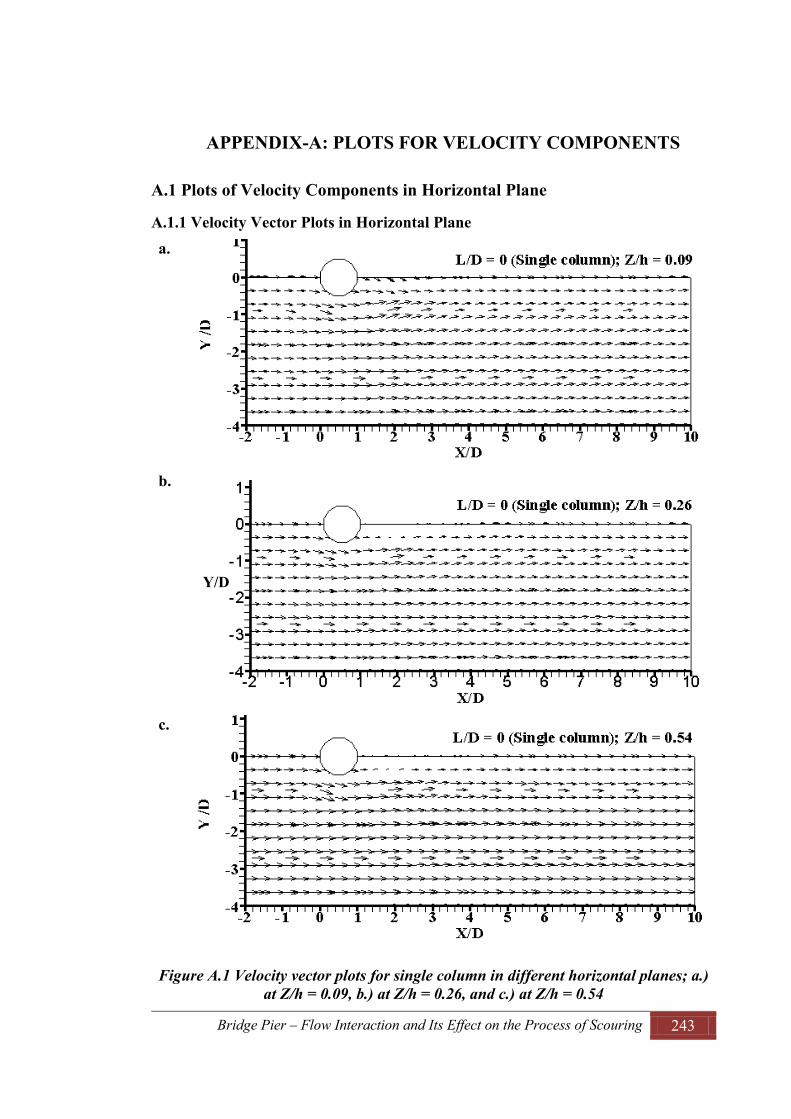
Bridge Pier – Flow Interaction and Its Effect on the Process of Scouring 243
APPENDIX-A: PLOTS FOR VELOCITY COMPONENTS
A.1 Plots of Velocity Components in Horizontal Plane
A.1.1 Velocity Vector Plots in Horizontal Plane a.
b.
c.
Figure A.1 Velocity vector plots for single column in different horizontal planes; a.) at Z/h = 0.09, b.) at Z/h = 0.26, and c.) at Z/h = 0.54
Y/D

Bridge Pier – Flow Interaction and Its Effect on the Process of Scouring 244
a.
b.
c.
Figure A.2 Velocity vector plots for two columns with L/D = 1.5 in different horizontal planes; a.) at Z/h = 0.09, b.) at Z/h = 0.26, and c.) at Z/h = 0.54
C1 C2
C1 C2

Bridge Pier – Flow Interaction and Its Effect on the Process of Scouring 245
a.
b.
c.
Figure A.3 Velocity vector plots for two columns with L/D = 2 in different horizontal planes; a.) at Z/h = 0.09, b.) at Z/h = 0.26, and c.) at Z/h = 0.54

Bridge Pier – Flow Interaction and Its Effect on the Process of Scouring 246
a.
b.
c.
Figure A.4 Velocity vector plots for two columns with L/D = 3 in different horizontal planes; a.) at Z/h = 0.09, b.) at Z/h = 0.26, and c.) at Z/h = 0.54
L/D = 3; Z/h = 0.09

Bridge Pier – Flow Interaction and Its Effect on the Process of Scouring 247
a.
b.
c.
Figure A.5 Velocity vector plots for two columns with L/D = 4 in different horizontal planes; a.) at Z/h = 0.09, b.) at Z/h = 0.26, and c.) at Z/h = 0.54

Bridge Pier – Flow Interaction and Its Effect on the Process of Scouring 248
A.1.2 Streamline Plots in Horizontal Plane a.
b.
c.
Figure A.6 Streamline plots for single column in different horizontal planes; a.) at Z/h = 0.09, b.) at Z/h = 0.26, and c.) at Z/h = 0.54
Y/D

Bridge Pier – Flow Interaction and Its Effect on the Process of Scouring 249
a.
b.
c.
Figure A.7 Streamline plots for two columns with L/D = 1.5 in different horizontal planes; a.) at Z/h = 0.09, b.) at Z/h = 0.26, and c.) at Z/h = 0.54

Bridge Pier – Flow Interaction and Its Effect on the Process of Scouring 250
a.
b.
c.
Figure A.8 Streamline plots for two columns with L/D = 2 in different horizontal planes; a.) at Z/h = 0.09, b.) at Z/h = 0.26, and c.) at Z/h = 0.54

Bridge Pier – Flow Interaction and Its Effect on the Process of Scouring 251
a.
b.
c.
Figure A.9 Streamline plots for two columns with L/D = 3 in different horizontal planes; a.) at Z/h = 0.09, b.) at Z/h = 0.26, and c.) at Z/h = 0.54
L/D = 3; Z/h = 0.09
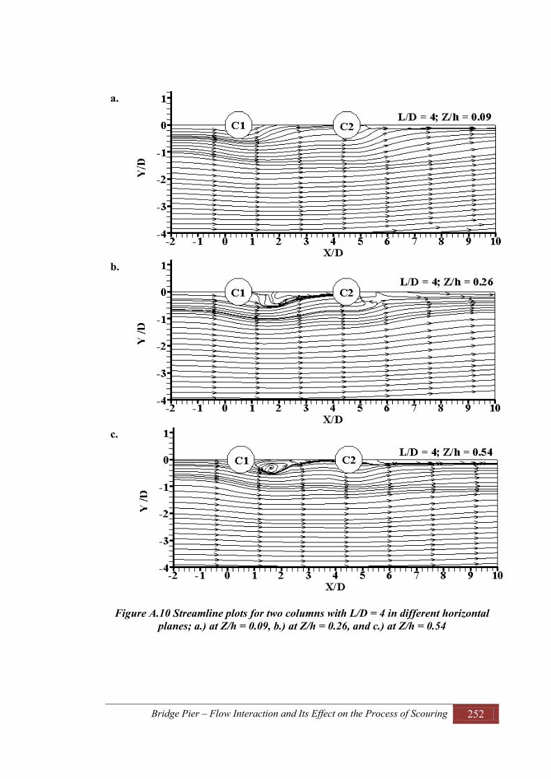
Bridge Pier – Flow Interaction and Its Effect on the Process of Scouring 252
a.
b.
c.
Figure A.10 Streamline plots for two columns with L/D = 4 in different horizontal planes; a.) at Z/h = 0.09, b.) at Z/h = 0.26, and c.) at Z/h = 0.54

Bridge Pier – Flow Interaction and Its Effect on the Process of Scouring 253
A.1.3 Contour Plots of Streamwise Velocity Component (u) in Horizontal Plane a.
b.
c.
Figure A.11 Contour plots of streamwise velocity component (u/V) for two columns with L/D = 1.5 in different horizontal planes; a.) at Z/h = 0.09, b.) at Z/h = 0.26, and
c.) at Z/h = 0.54

Bridge Pier – Flow Interaction and Its Effect on the Process of Scouring 254
a.
b.
c.
Figure A.12 Contour plots of streamwise velocity component (u/V) for two columns with L/D = 2 in different horizontal planes; a.) at Z/h = 0.09, b.) at Z/h = 0.26, and c.)
at Z/h = 0.54

Bridge Pier – Flow Interaction and Its Effect on the Process of Scouring 255
a.
b.
c.
Figure A.13 Contour plots of streamwise velocity component (u/V) for two columns with L/D = 4 in different horizontal planes; a.) at Z/h = 0.09, b.) at Z/h = 0.26, and c.)
at Z/h = 0.54
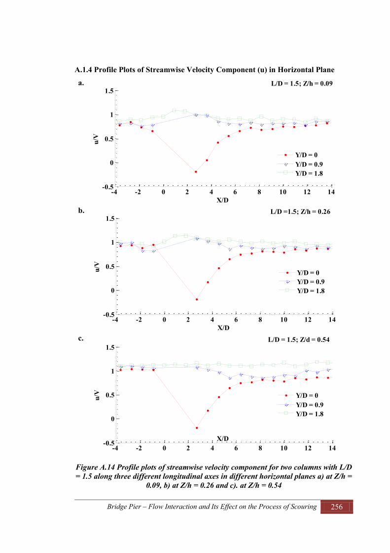
Bridge Pier – Flow Interaction and Its Effect on the Process of Scouring 256
A.1.4 Profile Plots of Streamwise Velocity Component (u) in Horizontal Plane a.
b.
c.
Figure A.14 Profile plots of streamwise velocity component for two columns with L/D = 1.5 along three different longitudinal axes in different horizontal planes a) at Z/h =
0.09, b) at Z/h = 0.26 and c). at Z/h = 0.54
-4 -2 0 2 4 6 8 10 12 14-0.5
0
0.5
1
1.5
X/D
u/V
L/D = 1.5; Z/h = 0.09
Y/D = 0Y/D = 0.9Y/D = 1.8
-4 -2 0 2 4 6 8 10 12 14-0.5
0
0.5
1
1.5
X/D
u/V
L/D =1.5; Z/h = 0.26
Y/D = 0Y/D = 0.9Y/D = 1.8
-4 -2 0 2 4 6 8 10 12 14-0.5
0
0.5
1
1.5
X/D
u/V
L/D = 1.5; Z/d = 0.54
Y/D = 0Y/D = 0.9Y/D = 1.8

Bridge Pier – Flow Interaction and Its Effect on the Process of Scouring 257
a.
b.
c.
Figure A.15 Profile plots of streamwise velocity component for two columns with L/D = 2 along three different longitudinal axes in different horizontal planes a) at Z/h =
0.09, b) at Z/h = 0.26 and c). at Z/h = 0.54
-4 -2 0 2 4 6 8 10 12 14-0.5
0
0.5
1
1.5
X/D
u/V
L/D = 2; Z/h = 0.09
data1data2data3
-4 -2 0 2 4 6 8 10 12 14-0.5
0
0.5
1
1.5
X/D
u/V
L/D = 2; Z/h = 0.26
Y/D = 0Y/D =0.9Y/D =1.8
-4 -2 0 2 4 6 8 10 12 14-0.5
0
0.5
1
1.5
X/D
u/V
L/D = 2; Z/h = 0.54
Y/D = 0Y/D = 0.9Y/D = 1.8

Bridge Pier – Flow Interaction and Its Effect on the Process of Scouring 258
a.
b.
c.
Figure A.16 Profile plots of streamwise velocity component for two columns with L/D = 4 along three different longitudinal axes in different horizontal planes a) at Z/h =
0.09, b) at Z/h = 0.26 and c). at Z/h = 0.54
-4 -2 0 2 4 6 8 10 12 14-0.5
0
0.5
1
1.5
X/D
u/V
L/D = 4; Z/h = 0.09
Y/D = 0Y/D = 0.9Y/D = 1.8
-4 -2 0 2 4 6 8 10 12 14-0.5
0
0.5
1
1.5
X/D
u/V
L/D = 4; Z/h = 0.26
Y/D = 0Y/D = 0.9Y/D = 1.8
-4 -2 0 2 4 6 8 10 12 14-0.5
0
0.5
1
1.5
X/D
u/V
L/D = 4; Z/h = 0.54
Y/D = 0Y/D = 0.9Y/D = 1.8

Bridge Pier – Flow Interaction and Its Effect on the Process of Scouring 259
a.
b.
c.
Figure A.17 Profile plots of streamwise velocity component for two columns with L/D = 6 along three different longitudinal axes in different horizontal planes a) at Z/h =
0.09, b) at Z/h = 0.26 and c). at Z/h = 0.54
-4 -2 0 2 4 6 8 10 12 14-0.5
0
0.5
1
1.5
X/D
u/V
L/D = 6; Z/h = 0.09
Y/D = 0Y/D = 0.9Y/D = 1.8
-4 -2 0 2 4 6 8 10 12 14-0.5
0
0.5
1
1.5
X/D
u/V
L/D = 6; Z/h = 0.26
Y/D = 0 Y/D = 0.9 Y/D = 1.8
-4 -2 0 2 4 6 8 10 12 14-0.5
0
0.5
1
1.5
X/D
u/V
L/D = 6; Z/h = 0.54
Y/D = 0Y/D = 0.9Y/D = 1.8

Bridge Pier – Flow Interaction and Its Effect on the Process of Scouring 260
A.1.5 Contour Plots of Transverse Velocity Component (v) in Horizontal Plane a.
b.
c.
Figure A.18 Contour plots of transverse velocity component (v/V) for two columns with L/D = 1.5 in different horizontal planes a) at Z/h = 0.09, b) at Z/h = 0.26 and c).
at Z/h = 0.54
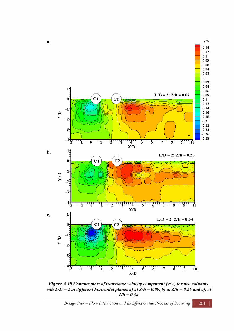
Bridge Pier – Flow Interaction and Its Effect on the Process of Scouring 261
a.
b.
c.
Figure A.19 Contour plots of transverse velocity component (v/V) for two columns with L/D = 2 in different horizontal planes a) at Z/h = 0.09, b) at Z/h = 0.26 and c). at
Z/h = 0.54

Bridge Pier – Flow Interaction and Its Effect on the Process of Scouring 262
a.
b.
c.
Figure A.19 Contour plots of transverse velocity component (v/V) for two columns with L/D = 4 in different horizontal planes a) at Z/h = 0.09, b) at Z/h = 0.26 and c). at
Z/h = 0.54

Bridge Pier – Flow Interaction and Its Effect on the Process of Scouring 263
A.1.6 Profile Plots of Transverse Velocity Component (v) in Horizontal Plane a.
b.
c.
Figure A.20 Profile plots of transverse velocity component for two columns with L/D = 1.5 along three different longitudinal axes in different horizontal planes a) at Z/h =
0.09, b) at Z/h = 0.26 and c). at Z/h = 0.54
-4 -2 0 2 4 6 8 10 12 14-0.1
0
0.1
0.2
0.3
X/D
v/V
L/D = 1.5; Z/h = 0.09
Y/D = 0Y/D = 0.9Y/D = 1.8
-4 -2 0 2 4 6 8 10 12 14-0.1
0
0.1
0.2
0.3
X/D
v/V
L/D = 1.5; Z/h= 0.26
Y/D = 0Y/D = 0.9Y/D = 1.8
-4 -2 0 2 4 6 8 10 12 14-0.1
0
0.1
0.2
0.3
X/D
v/V
L/D = 1.5; Z/h= 0.54
Y/D = 0Y/D = 0.9Y/D = 1.8

Bridge Pier – Flow Interaction and Its Effect on the Process of Scouring 264
a.
b.
c.
Figure A.21 Profile plots of transverse velocity component for two columns with L/D = 2 along three different longitudinal axes in different horizontal planes a) at Z/h =
0.09, b) at Z/h = 0.26 and c). at Z/h = 0.54
-4 -2 0 2 4 6 8 10 12 14-0.4
-0.2
0
0.2
0.4
X/D
v/V
L/D = 2; Z/h= 0.09
Y/D = 0Y/D = 0.9Y/D = 1.8
-4 -2 0 2 4 6 8 10 12 14-0.4
-0.2
0
0.2
0.4
X/D
v/V
L/D = 2; Z/h= 0.26
Y/D = 0Y/D = 0.9Y/D = 1.8
-4 -2 0 2 4 6 8 10 12 14-0.4
-0.2
0
0.2
0.4
X/D
v/V
L/D = 2; Z/h= 0.54
Y/D = 0Y/D = 0.9Y/D = 1.8

Bridge Pier – Flow Interaction and Its Effect on the Process of Scouring 265
a.
b.
c.
Figure A.23 Profile plots of transverse velocity component for two columns with L/D = 4 along three different longitudinal axes in different horizontal planes a) at Z/h =
0.09, b) at Z/h = 0.26 and c). at Z/h = 0.54
-4 -2 0 2 4 6 8 10 12 14-0.4
-0.2
0
0.2
0.4
X/D
v/V
L/D = 4; Z/h = 0.09
Y/D = 0Y/D = 0.9Y/D = 1.8
-4 -2 0 2 4 6 8 10 12 14-0.4
-0.2
0
0.2
0.4
X/D
v/V
L/D = 4; Z/h = 0.26
Y/D = 0Y/D = 0.9Y/D = 1.8
-4 -2 0 2 4 6 8 10 12 14-0.4
-0.2
0
0.2
0.4
X/D
v/V
L/D = 4; Z/h = 0.54
Y/D = 0Y/D = 0.9Y/D = 1.8
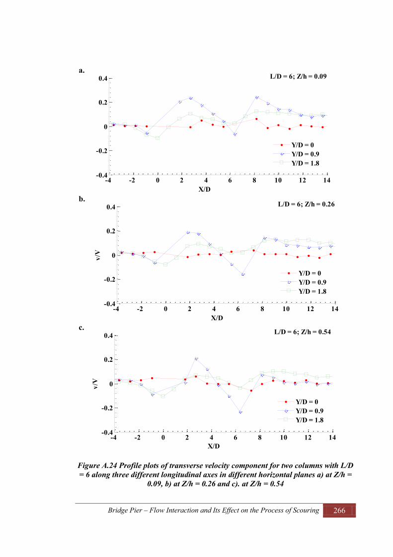
Bridge Pier – Flow Interaction and Its Effect on the Process of Scouring 266
a.
b.
c.
Figure A.24 Profile plots of transverse velocity component for two columns with L/D = 6 along three different longitudinal axes in different horizontal planes a) at Z/h =
0.09, b) at Z/h = 0.26 and c). at Z/h = 0.54
-4 -2 0 2 4 6 8 10 12 14-0.4
-0.2
0
0.2
0.4
X/D
L/D = 6; Z/h = 0.09
Y/D = 0Y/D = 0.9Y/D = 1.8
-4 -2 0 2 4 6 8 10 12 14-0.4
-0.2
0
0.2
0.4
X/D
v/V
L/D = 6; Z/h = 0.26
Y/D = 0Y/D = 0.9Y/D = 1.8
-4 -2 0 2 4 6 8 10 12 14-0.4
-0.2
0
0.2
0.4
X/D
v/V
L/D = 6; Z/h = 0.54
Y/D = 0Y/D = 0.9Y/D = 1.8
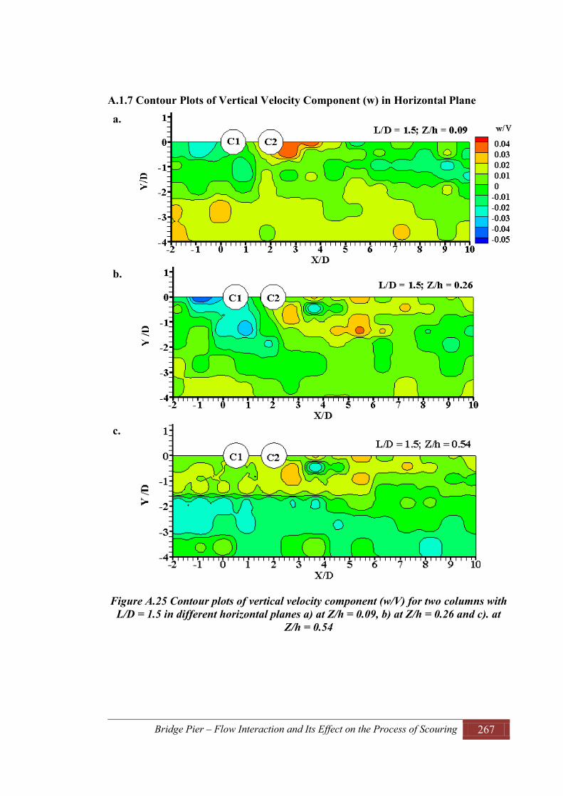
Bridge Pier – Flow Interaction and Its Effect on the Process of Scouring 267
A.1.7 Contour Plots of Vertical Velocity Component (w) in Horizontal Plane a.
b.
c.
Figure A.25 Contour plots of vertical velocity component (w/V) for two columns with L/D = 1.5 in different horizontal planes a) at Z/h = 0.09, b) at Z/h = 0.26 and c). at
Z/h = 0.54
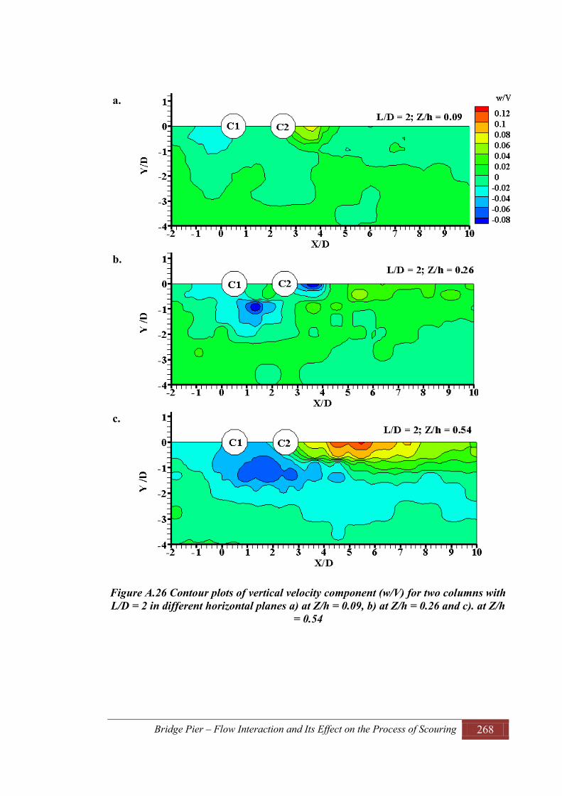
Bridge Pier – Flow Interaction and Its Effect on the Process of Scouring 268
a.
b.
c.
Figure A.26 Contour plots of vertical velocity component (w/V) for two columns with L/D = 2 in different horizontal planes a) at Z/h = 0.09, b) at Z/h = 0.26 and c). at Z/h
= 0.54

Bridge Pier – Flow Interaction and Its Effect on the Process of Scouring 269
a.
b.
c.
Figure A.27 Contour plots of vertical velocity component (w/V) for two columns with L/D = 4 in different horizontal planes a) at Z/h = 0.09, b) at Z/h = 0.26 and c). at Z/h
= 0.54

Bridge Pier – Flow Interaction and Its Effect on the Process of Scouring 270
A.1.8 Profile Plots of Vertical Velocity Component (w) in Horizontal Plane a.
b.
c.
Figure A.28 Profile plots of vertival velocity component for two columns with L/D = 1.5 along three different longitudinal axes in different horizontal planes a) at Z/h =
0.09, b) at Z/h = 0.26 and c). at Z/h = 0.54
-4 -2 0 2 4 6 8 10 12 14-0.06
-0.04
-0.02
0
0.02
0.04
0.06
X/D
w/V
L/D = 1.5; Z/h = 0.09
Y/D = 0Y/D = 0.9Y/D = 1.8
-4 -2 0 2 4 6 8 10 12 14-0.06
-0.04
-0.02
0
0.02
0.04
0.06
X/D
w/V
L/D = 1.5; Z/h = 0.26
Y/D = 0Y/D = 0.9Y/D = 1.8
-4 -2 0 2 4 6 8 10 12 14-0.06
-0.04
-0.02
0
0.02
0.04
0.06
X/D
w/V
L/D = 1.5; Z/h = 0.54
Y/D = 0Y/D = 0.9Y/D = 1.8

Bridge Pier – Flow Interaction and Its Effect on the Process of Scouring 271
a.
b.
c.
Figure A.29 Profile plots of vertival velocity component for two columns with L/D = 2 along three different longitudinal axes in different horizontal planes a) at Z/h = 0.09,
b) at Z/h = 0.26 and c). at Z/h = 0.54
-4 -2 0 2 4 6 8 10 12 14-0.1
-0.05
0
0.05
0.1
0.15
X/D
w/V
L/D = 2; Z/h = 0.09
Y/D = 0Y/D = 0.9Y/D = 1.8
-4 -2 0 2 4 6 8 10 12 14-0.1
-0.05
0
0.05
0.1
0.15
X/D
w/V
L/D = 2; Z/h = 0.26
Y/D = 0Y/D = 0.9Y/D = 1.8
-4 -2 0 2 4 6 8 10 12 14-0.1
-0.05
0
0.05
0.1
0.15
X/D
w/V
L/D = 2; Z/h = 0.54
Y/D = 0Y/D = 0.9Y/D = 1.8

Bridge Pier – Flow Interaction and Its Effect on the Process of Scouring 272
a.
b.
c.
Figure A.30 Profile plots of vertival velocity component for two columns with L/D = 4 along three different longitudinal axes in different horizontal planes a) at Z/h = 0.09,
b) at Z/h = 0.26 and c). at Z/h = 0.54
-4 -2 0 2 4 6 8 10 12 14-0.2
-0.1
0
0.1
0.2
0.3
0.4
X/D
w/V
L/D = 4; Z/h = 0.09
Y/D = 0Y/D = 0.9Y/D = 1.8
-4 -2 0 2 4 6 8 10 12 14-0.2
-0.1
0
0.1
0.2
0.3
0.4
X/D
w/V
L/D = 4; Z/h = 0.26
Y/D = 0Y/D = 0.9Y/D = 1.8
-4 -2 0 2 4 6 8 10 12 14-0.2
-0.1
0
0.1
0.2
0.3
0.4
X/D
w/V
L/D = 4; Z/h = 0.54
Y/D = 0Y/D = 0.9Y/D = 1.8

Bridge Pier – Flow Interaction and Its Effect on the Process of Scouring 273
a.
b.
c.
Figure A.31 Profile plots of vertival velocity component for two columns with L/D = 6 along three different longitudinal axes in different horizontal planes a) at Z/h = 0.09,
b) at Z/h = 0.26 and c). at Z/h = 0.54
-4 -2 0 2 4 6 8 10 12 14-0.2
-0.1
0
0.1
0.2
X/D
w/V
L/D = 6; Z/h = 0.09
Y/D = 0Y/D = 0.9Y/D = 1.8
-4 -2 0 2 4 6 8 10 12 14-0.2
-0.1
0
0.1
0.2
X/D
w/V
L/D = 6; Z/h = 0.26
Y/D = 0Y/D = 0.9Y/D = 1.8
-4 -2 0 2 4 6 8 10 12 14-0.2
-0.1
0
0.1
0.2
X/D
w/V
L/D = 6; Z/h = 0.54
Y/D = 0Y/D = 0.9Y/D = 1.8

Bridge Pier – Flow Interaction and Its Effect on the Process of Scouring 274
A.2 Plots of Velocity Components for Vertical Plane.
A.2.1 Velocity Vector Plots in Vertical Plane a.
b.
Figure A.32 Vector plots for two columns case with L/D = 1 in different vertical planes; a.) at Y/D = 0, and b.) at Y/D = 1.25
C1 C2 L/D = 1; Y/D =0
C1 C2

Bridge Pier – Flow Interaction and Its Effect on the Process of Scouring 275
a.
b.
Figure A.33 Vector plots for two columns case with L/D = 2 in different vertical planes; a.) at Y/D = 0, and b.) at Y/D = 1.25
C1 C2
C1 C2 1.25

Bridge Pier – Flow Interaction and Its Effect on the Process of Scouring 276
a.
b.
Figure A.34 Vector plots for two columns case with L/D = 4 in different vertical planes; a.) at Y/D = 0, and b.) at Y/D = 1.25
C1 C2
C1 C2
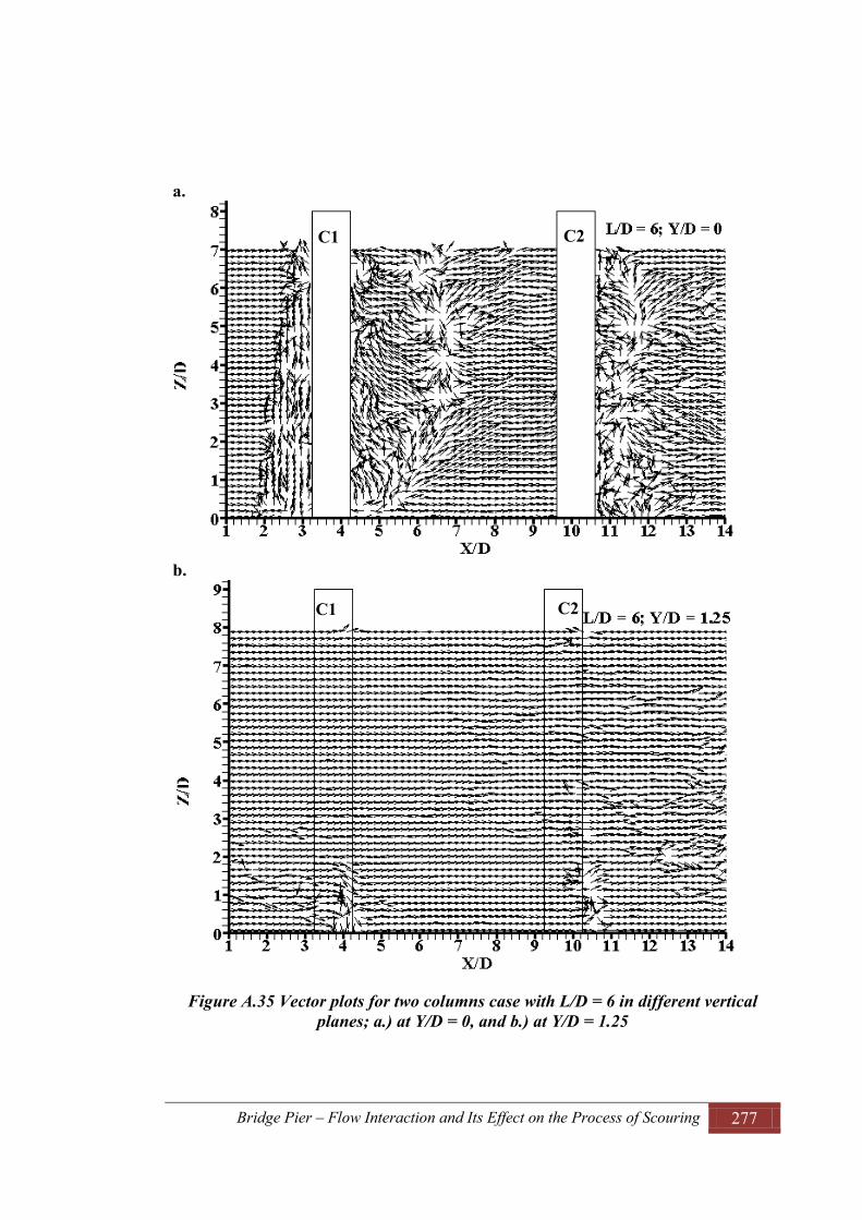
Bridge Pier – Flow Interaction and Its Effect on the Process of Scouring 277
a.
b.
Figure A.35 Vector plots for two columns case with L/D = 6 in different vertical planes; a.) at Y/D = 0, and b.) at Y/D = 1.25
C1 C2
C1 C2

Bridge Pier – Flow Interaction and Its Effect on the Process of Scouring 278
A.2.2 Stream Line Plots in Vertical Plane a.
b.
Figure A.36 Streamline plots for two columns case with L/D = 1 in different vertical planes; a.) at Y/D = 0, and b.) at Y/D = 1.25
C1 C2
C1 C2

Bridge Pier – Flow Interaction and Its Effect on the Process of Scouring 279
a.
b.
Figure A.37 Streamline plots for two columns case with L/D = 2 in different vertical planes; a.) at Y/D = 0, and b.) at Y/D = 1.25
C1 C2
C1 C2

Bridge Pier – Flow Interaction and Its Effect on the Process of Scouring 280
a.
b.
Figure A.38 Streamline plots for two columns case with L/D = 4 in different vertical planes; a.) at Y/D = 0, and b.) at Y/D = 1.25
C1 C2
C1 C2

Bridge Pier – Flow Interaction and Its Effect on the Process of Scouring 281
a.
b.
Figure A.39 Streamline plots for two columns case with L/D = 6 in different vertical planes; a.) at Y/D = 0, and b.) at Y/D = 1.25
C1 C2
C1 C2

Bridge Pier – Flow Interaction and Its Effect on the Process of Scouring 282
A.2.3 Contour Plots of Streamwise velocity components (u) in Vertical Plane a.
b.
Figure A.40 Contour plots of streamwise velocity component (u/V) for two columns with L/D = 1 in different vertical planes a) at Y/D = 0, b) at Y/D = 1.25
C1 C2
C1 C2
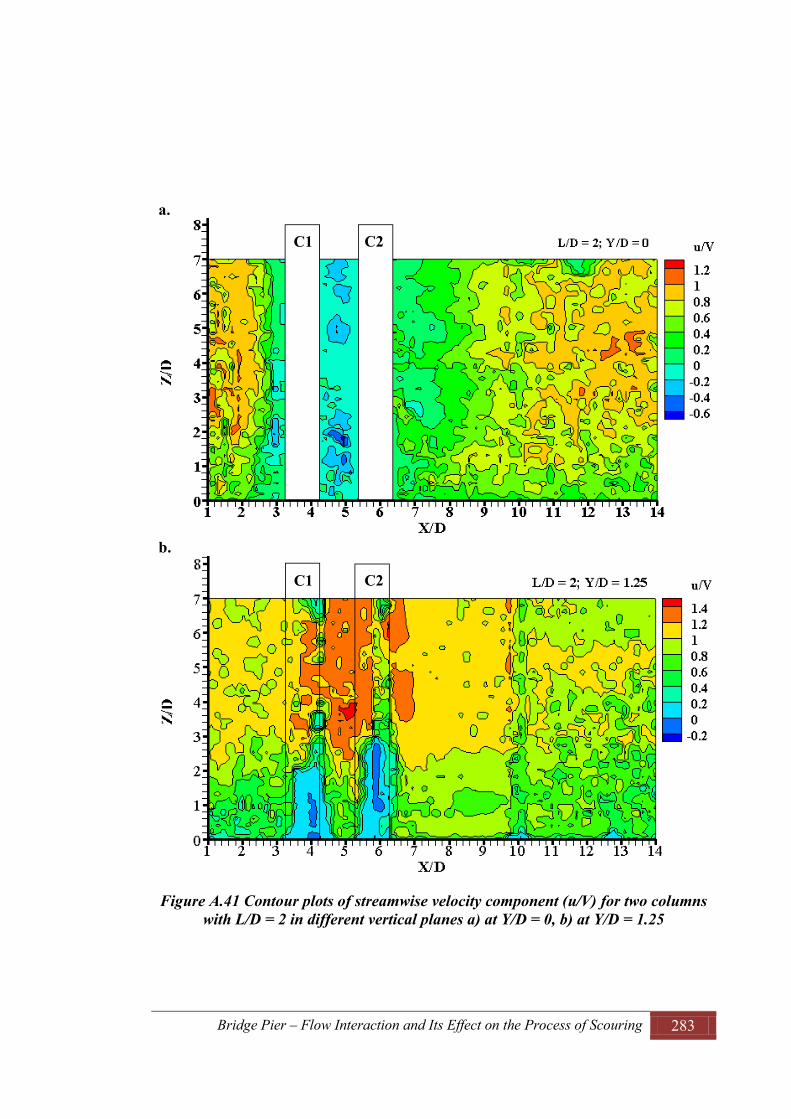
Bridge Pier – Flow Interaction and Its Effect on the Process of Scouring 283
a.
b.
Figure A.41 Contour plots of streamwise velocity component (u/V) for two columns with L/D = 2 in different vertical planes a) at Y/D = 0, b) at Y/D = 1.25
C1 C2
C1 C2

Bridge Pier – Flow Interaction and Its Effect on the Process of Scouring 284
a.
b.
Figure A.42 Contour plots of streamwise velocity component (u/V) for two columns with L/D = 4 in different vertical planes a) at Y/D = 0, b) at Y/D = 1.25
C1 C2
C1 C2 ;

Bridge Pier – Flow Interaction and Its Effect on the Process of Scouring 285
a.
b.
Figure A.43 Contour plots of streamwise velocity component (u/V) for two columns with L/D = 6 in different vertical planes a) at Y/D = 0, b) at Y/D = 1.25
C1 C2
C1 C2
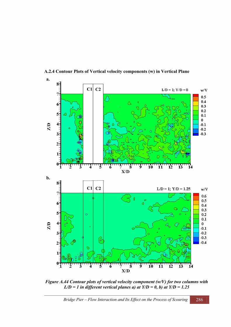
Bridge Pier – Flow Interaction and Its Effect on the Process of Scouring 286
A.2.4 Contour Plots of Vertical velocity components (w) in Vertical Plane a.
b.
Figure A.44 Contour plots of vertical velocity component (w/V) for two columns with L/D = 1 in different vertical planes a) at Y/D = 0, b) at Y/D = 1.25
C1 C2
C1 C2

Bridge Pier – Flow Interaction and Its Effect on the Process of Scouring 287
a.
b.
Figure A.45 Contour plots of vertical velocity component (w/V) for two columns with L/D = 2 in different vertical planes a) at Y/D = 0, b) at Y/D = 1.25
C1 C2
C1 C2

Bridge Pier – Flow Interaction and Its Effect on the Process of Scouring 288
a.
b.
Figure A.46 Contour plots of vertical velocity component (w/V) for two columns with L/D = 4 in different vertical planes a) at Y/D = 0, b) at Y/D = 1.25
C1 C2
C1 C2

Bridge Pier – Flow Interaction and Its Effect on the Process of Scouring 289
a.
b.
Figure A.47 Contour plots of vertical velocity component (w/V) for two columns with L/D = 6 in different vertical planes a) at Y/D = 0, b) at Y/D = 1.25
C1 C2
C1 C2

Bridge Pier – Flow Interaction and Its Effect on the Process of Scouring 290
A.2.5 Profile Plots of Velocity Components at Upstream and Downstream Side (at Y=0) in Vertical Plane
a. b.
Figure A.48 Profile plots of streamwise velocity component for two columns case with L/D = 1 a in vertical plane at axis of symmetry a) upstream side; b) downstream side
a. b.
Figure A.49 Profile plots of vertical velocity component for two columns case with L/D = 1 a in vertical plane at axis of symmetry a) upstream side; b) downstream side
0 0.5 1 1.50
1
2
3
4
5
6
7
u/V
Z/D
US1US2
0 0.5 10
1
2
3
4
5
6
7
u/V
Z/D
DS1DS2DS4
-0.2 0 0.20
1
2
3
4
5
6
7
w/V
Z/D
US1US2
-0.5 0 0.50
1
2
3
4
5
6
7
w/V
Z/D
DS1DS2DS4

Bridge Pier – Flow Interaction and Its Effect on the Process of Scouring 291
a. b.
Figure A.50 Profile plots of streamwise velocity component for two columns case with L/D = 2 a in vertical plane at axis of symmetry a) upstream side; b) downstream side
a. b.
Figure A.51 Profile plots of vertical velocity component for two columns case with L/D = 2 a in vertical plane at axis of symmetry a) upstream side; b) downstream side
0 0.5 1 1.50
1
2
3
4
5
6
7
u/V
Z/D
US1US2
-0.5 0 0.5 10
1
2
3
4
5
6
7
u/VZ/
D
DS1DS2DS4
-0.5 0 0.50
1
2
3
4
5
6
7
w/V
Z/D
US1US2
-0.5 0 0.50
1
2
3
4
5
6
7
w/V
Z/D
DS1DS2DS4

Bridge Pier – Flow Interaction and Its Effect on the Process of Scouring 292
a. b.
Figure A.52 Profile plots of velocity components between two columns with L/D = 2 in vertical plane at axis of symmetry a) stream wise component, b) vertical component
a. b.
Figure A.53 Profile plots of streamwise velocity component for two columns case with L/D = 4 a in vertical plane at axis of symmetry a) upstream side; b) downstream side
-1 -0.5 0 0.50
1
2
3
4
5
6
7
u/V
Z/D
B1
-0.5 0 0.5 10
1
2
3
4
5
6
7
w/VZ/
D
B1
0 0.5 1 1.50
1
2
3
4
5
6
7
u/V
Z/D
US1US2
-0.5 0 0.5 10
1
2
3
4
5
6
7
u/V
Z/D
DS1DS2DS3
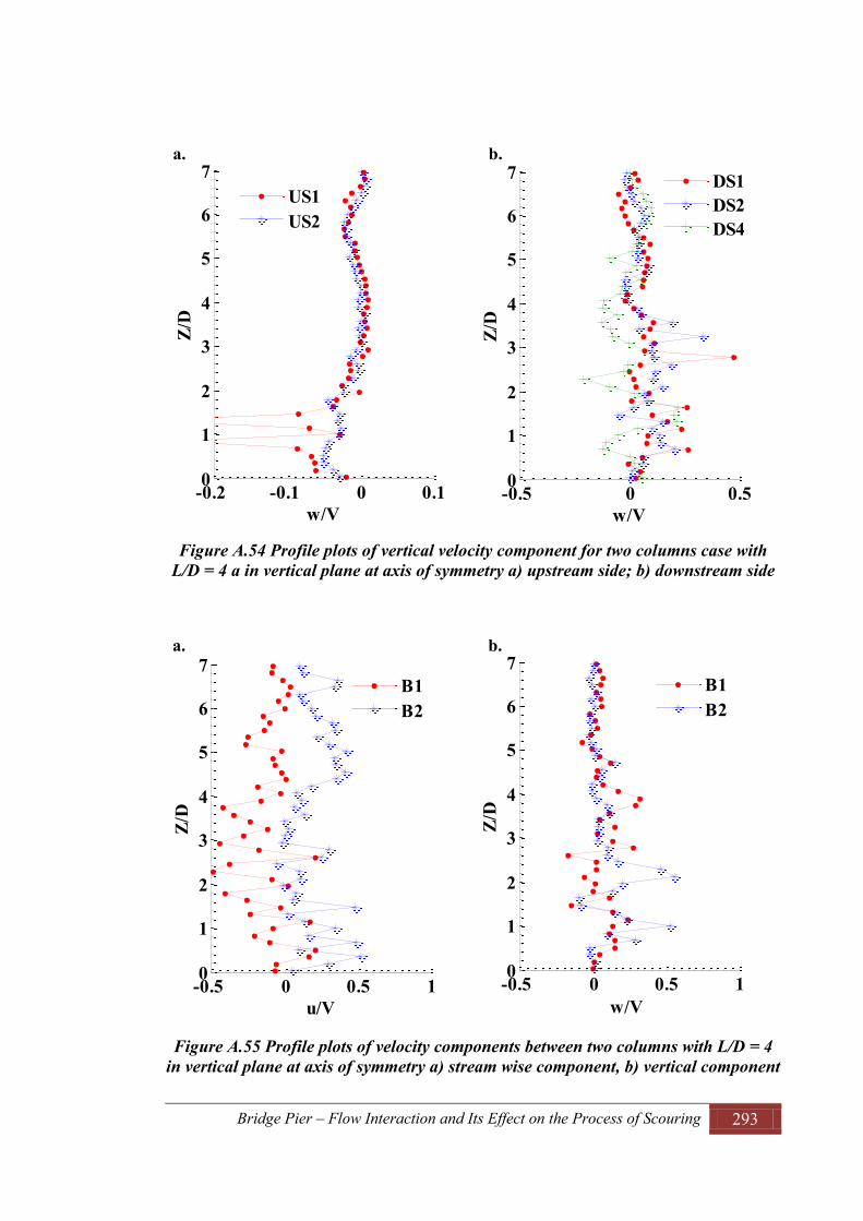
Bridge Pier – Flow Interaction and Its Effect on the Process of Scouring 293
a. b.
Figure A.54 Profile plots of vertical velocity component for two columns case with L/D = 4 a in vertical plane at axis of symmetry a) upstream side; b) downstream side
a. b.
Figure A.55 Profile plots of velocity components between two columns with L/D = 4 in vertical plane at axis of symmetry a) stream wise component, b) vertical component
-0.2 -0.1 0 0.10
1
2
3
4
5
6
7
w/V
Z/D
US1US2
-0.5 0 0.50
1
2
3
4
5
6
7
w/VZ/
D
DS1DS2DS4
-0.5 0 0.5 10
1
2
3
4
5
6
7
u/V
Z/D
B1B2
-0.5 0 0.5 10
1
2
3
4
5
6
7
w/V
Z/D
B1B2
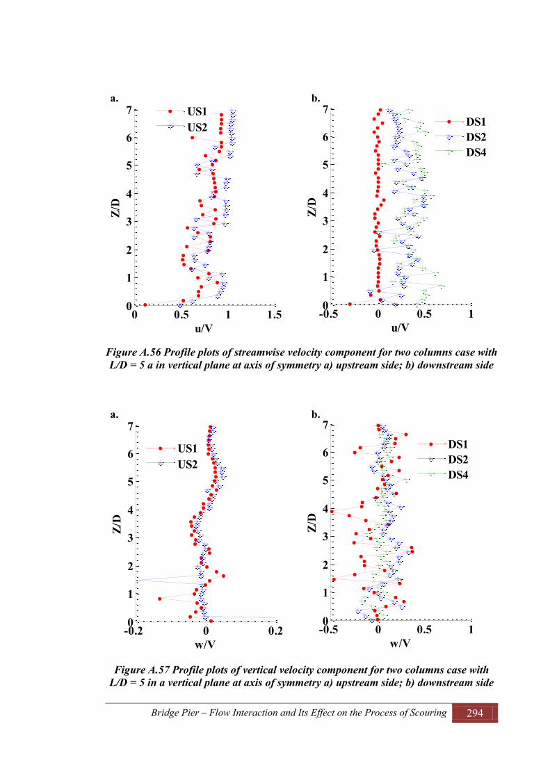
Bridge Pier – Flow Interaction and Its Effect on the Process of Scouring 294
a. b.
Figure A.56 Profile plots of streamwise velocity component for two columns case with L/D = 5 a in vertical plane at axis of symmetry a) upstream side; b) downstream side
a. b.
Figure A.57 Profile plots of vertical velocity component for two columns case with L/D = 5 in a vertical plane at axis of symmetry a) upstream side; b) downstream side
0 0.5 1 1.50
1
2
3
4
5
6
7
u/V
Z/D
US1US2
-0.5 0 0.5 10
1
2
3
4
5
6
7
u/VZ/
D
DS1DS2DS4
-0.2 0 0.20
1
2
3
4
5
6
7
w/V
Z/D
US1US2
-0.5 0 0.5 10
1
2
3
4
5
6
7
w/V
Z/D
DS1DS2DS4

Bridge Pier – Flow Interaction and Its Effect on the Process of Scouring 295
a. b.
Figure A.58 Profile plots of velocity components between two columns with L/D = 5 in vertical plane at axis of symmetry a) streamwise component, b) vertical component
a. b.
Figure A.59 Profile plots of streamwise velocity component for two columns case with L/D = 6 a in vertical plane at axis of symmetry a) upstream side; b) downstream side
-0.5 0 0.5 10
1
2
3
4
5
6
7
u/V
Z/D
B1B2B3
-0.5 0 0.5 10
1
2
3
4
5
6
7
w/VZ/
D
B1B2B3
-1 0 1 20
1
2
3
4
5
6
7
u/V
Z/D
US1US2
-0.5 0 0.5 1 1.50
1
2
3
4
5
6
7
u/V
Z/D
DS1DS2DS4
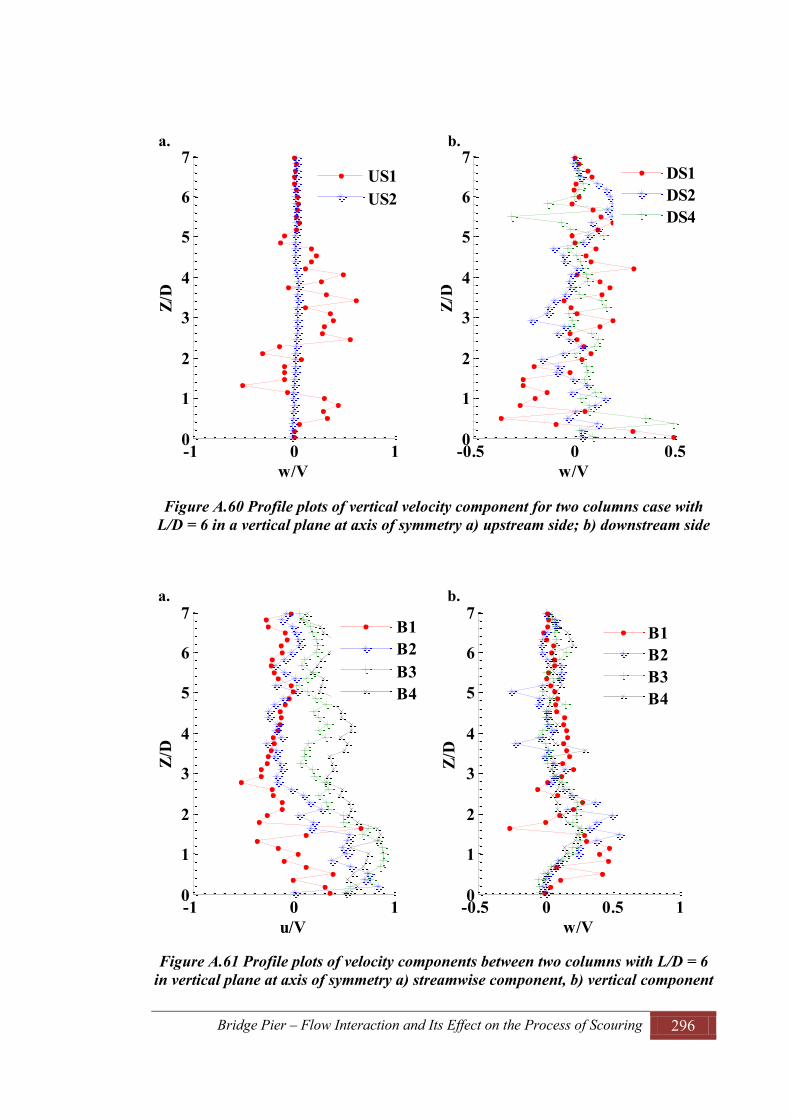
Bridge Pier – Flow Interaction and Its Effect on the Process of Scouring 296
a. b.
Figure A.60 Profile plots of vertical velocity component for two columns case with L/D = 6 in a vertical plane at axis of symmetry a) upstream side; b) downstream side
a. b.
Figure A.61 Profile plots of velocity components between two columns with L/D = 6 in vertical plane at axis of symmetry a) streamwise component, b) vertical component
-1 0 10
1
2
3
4
5
6
7
w/V
Z/D
US1US2
-0.5 0 0.50
1
2
3
4
5
6
7
w/VZ/
D
DS1DS2DS4
-1 0 10
1
2
3
4
5
6
7
u/V
Z/D
B1B2B3B4
-0.5 0 0.5 10
1
2
3
4
5
6
7
w/V
Z/D
B1B2B3B4

Bridge Pier – Flow Interaction and Its Effect on the Process of Scouring 297
A.3 Table of Results on Velocity Components Table A. 1 Maximum and minimum values of streamwise velocity components
Test No.
L/D Z/h Y/D umax/V X/D umin/V X/D
1 0
0.09 0 0.9 -4 0.65 2 0.9 1.2 2 0.6 -1 1.8 1.1 1 0.9 -1
0.26 0 0.9 -4 -0.1 2 0.9 1.3 2 0.9 3.5 1.8 1.1 2 0.9 -2
0.54 0 1 -4 -0.2 2 0.9 1.3 2 1 3.5 1.8 1.2 2 1 3.5
2 1.5
0.09 0 0.9 -4 -0.2 3 0.9 1 3 0.8 6.5 1.8 1.1 1 0.9 7
0.26 0 0.9 -4 -0.2 3 0.9 1.1 3 0.9 5.5 1.8 1.15 1.5 0.9 7
0.54 0 1 -4 -0.2 3 0.9 1.1 3 0.8 6 1.8 1.2 3 1 6
3 2
0.09 0 0.8 -4 0.1 1 0.9 1.1 2 0.7 4 1.8 1 2 0.8 7
0.26 0 0.9 -4 -0.1 3.5 0.9 1.2 1.5 0.9 9 1.8 1.1 2 0.9 7
0.54 0 0.9 -4 0 3.5 0.9 1.1 2.5 0.9 7.5 1.8 1.25 2 1.1 11
4 3
0.09 0 0.9 -4 -0.25 2 0.9 1.2 2 0.8 5.5 1.8 1.15 1.5 0.75 9
0.26 0 1 -4 -0.3 2.5 0.9 1.2 2.5 0.8 7 1.8 1.2 1.5 0.9 5.5
0.54 0 1 -4 -0.3 2 0.9 1.4 1.5 0.9 9 1.8 1.2 2 1.1 12
5 4 0.09 0 0.9 -4 -0.1 5.5 0.9 1.2 1 0.8 11 1.8 1.1 1 0.95 9
0.26 0 1 -4 -0.1 5.5

Bridge Pier – Flow Interaction and Its Effect on the Process of Scouring 298
0.9 1.25 2 0.9 10 1.8 1.15 2 1 12
0.54 0 1 -4 -0.3 2 0.9 1.3 1.5 0.8 9 1.8 1.2 1 1 11
6 6
0.09 0 0.9 -4 0.2 8 0.9 1.2 2 0.8 -1 1.8 1 2 0.9 -2
0.26 0 1 -4 -0.2 7 0.9 1.1 2 0.8 -2 1.8 1.2 1 0.9 -2
0.54 0 1 -4 -0.2 2, 7 0.9 1 7 0.7 2 1.8 1.2 1 1 -1

Bridge Pier – Flow Interaction and Its Effect on the Process of Scouring 299
Table A. 2 Maximum and minimum values of transverse velocity components
Test No.
L/D Z/h Y/D vmax/V X/D vmin/V X/D
1 0
0.09 0 0 -4 -0.15 2 0.9 0.35 2 -0.2 0 1.8 0.15 3 -0.1 0
0.26 0 0 -4 -0.1 2 0.9 0.18 2 -0.2 0 1.8 0 -4 -0.1 0
0.54 0 0 -4 0.02 2 0.9 0.1 3 -0.3 3 1.8 0.05 3 -0.05 0
2 1.5
0.09 0 0.02 5.5 0 -4 0.9 0.1 4 -0.05 -1 1.8 0.1 4 -0.08 0
0.26 0 0 -4 -0.08 3 0.9 0.18 4 -0.07 -1 1.8 0.1 4 -0.08 0
0.54 0 0.05 -4 -0.08 2.5 0.9 0.18 4 0 -1 1.8 0 0
3 2
0.09 0 0 -4 -0.1 1 0.9 0.18 4 -0.21 0 1.8 0.1 4 -0.1 1
0.26 0 0 0 0.9 0.15 4 -0.02 -1 1.8 0.1 4 -0.04 0
0.54 0 0.03 5 3 0.9 0.18 4 -0.3 0 1.8 0.1 5 -0.1 0
4 3
0.09 0 0.1 4 0 0.9 0.1 5 -0.22 0 1.8 0.1 5.5 -0.1 0
0.26 0 0 0 0.9 0.2 5 -0.3 0 1.8 0.15 5 -0.1 0
0.54 0 0 0 0.9 0.2 5 -0.25 0 1.8 0.15 4 -0.18 0
5 4
0.09 0 0.04 2 0 0.9 0.2 5.5 -0.18 0 1.8 0.15 6 -0.1 0
0.26 0 0 -0.1 3 0.9 0.2 6 -0.2 0 1.8 0.18 6.5 -0.1 0

Bridge Pier – Flow Interaction and Its Effect on the Process of Scouring 300
0.54 0 0 -0.1 5.5 0.9 0.08 6.5 -0.28 0 1.8 0.1 7 -0.1 0
6 6
0.09 0 0 0 0.9 0.24 8 -0.05 6 1.8 0.12 8 -0.08 0
0.26 0 0 0 0.9 0.2 2 -0.18 6 1.8 0.15 8 -0.06 8
0.54 0 0 0 0.9 0.22 3 -0.24 6 1.8 0.1 9 -0.1 0

Bridge Pier – Flow Interaction and Its Effect on the Process of Scouring 301
Table A. 3 Maximum and minimum values of vertical velocity components
Test No.
L/D Z/h Y/D wmax/V X/D wmin/V X/D
1 0
0.09 0 0.22 2 -0.05 -1 0.9 0.05 3 -0.05 0 1.8 0.05 1 -0.02 -1
0.26 0 0.23 2.5 -0.02 -1 0.9 0.06 6 -0.05 2 1.8 0 -0.06 6
0.54 0 0.14 4 -0.04 -1 0.9 0.05 8 -0.08 2 1.8 0 -0.1 6
2 1.5
0.09 0 0.04 3 -0.025 -1 0.9 0.01 13 -0.02 9 1.8 0.015 5.5 0 -4
0.26 0 0.03 5.5 -0.05 -1 0.9 0.03 6 -0.02 -3 1.8 0.01 4.5 -0.02 2
0.54 0 0.03 5.5 0 3 0.9 0.03 5.5 0 3 1.8 0 5.5 -0.03 -1
3 2
0.09 0 0.08 1 -0.03 -1 0.9 0 4 -0.03 -1 1.8 0 0
0.26 0 0.04 6 -0.1 3.5 0.9 0.03 3.5 -0.08 1.5 1.8 0 0
0.54 0 0.12 5.5 -0.03 -1 0.9 0.03 6 -0.05 0 1.8 0 -1 -0.04 3
4 3
0.09 0 0.27 3.5 -0.02 -1 0.9 0.05 3 -0.03 0 1.8 0 0
0.26 0 0.18 2.5 -0.01 -1 0.9 0 -0.07 2.5 1.8 0 0
0.54 0 0.35 2 0 0.9 0.03 5.5 -0.1 2 1.8 0 0
5 4
0.09 0 0.18 5.5 -0.05 2.5 0.9 0.02 4 -0.05 0 1.8 0 0
0.26 0 0.35 2 -0.05 -1 0.9 0.02 5.5 -0.1 2 1.8 0 0

Bridge Pier – Flow Interaction and Its Effect on the Process of Scouring 302
0.54 0 0.18 2.5 -0.1 5.5 0.9 0.07 6 -0.1 2 1.8 0 0
6 6
0.09 0 0.1 2.5 -0.02 -1 0.9 0 0 1.8 0 0
0.26 0 0.17 3.5 -0.05 -1 0.9 0.05 5.5 -0.05 2 1.8 0 0
0.54 0 0.18 5.5 -0.16 7 0.9 0.15 6 0.05 2 1.8 0 -0.1 4.5
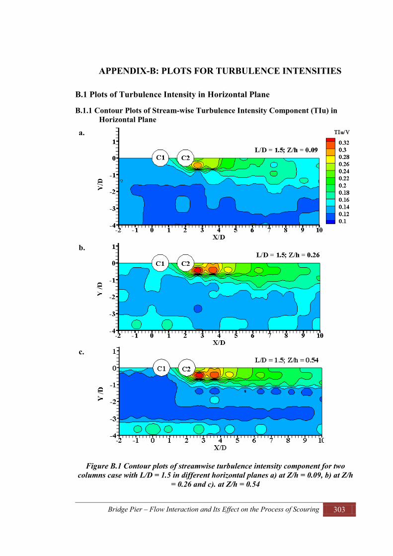
Bridge Pier – Flow Interaction and Its Effect on the Process of Scouring 303
APPENDIX-B: PLOTS FOR TURBULENCE INTENSITIES
B.1 Plots of Turbulence Intensity in Horizontal Plane
B.1.1 Contour Plots of Stream-wise Turbulence Intensity Component (TIu) in Horizontal Plane
a.
b.
c.
Figure B.1 Contour plots of streamwise turbulence intensity component for two columns case with L/D = 1.5 in different horizontal planes a) at Z/h = 0.09, b) at Z/h
= 0.26 and c). at Z/h = 0.54

Bridge Pier – Flow Interaction and Its Effect on the Process of Scouring 304
a.
b.
c.
Figure B.2 Contour plots of streamwise turbulence intensity component for two columns case with L/D = 2 in different horizontal planes a) at Z/h = 0.09, b) at Z/h =
0.26 and c). at Z/h = 0.54

Bridge Pier – Flow Interaction and Its Effect on the Process of Scouring 305
a.
b.
c.
Figure B.3 Contour plots of streamwise turbulence intensity component for two columns case with L/D = 4 in different horizontal planes a) at Z/h = 0.09, b) at Z/h =
0.26 and c). at Z/h = 0.54

Bridge Pier – Flow Interaction and Its Effect on the Process of Scouring 306
B.1.2 Profile Plots of Stream-wise Turbulence Intensity Component (TIu) in Horizontal Plane
a.
b.
c.
Figure B.4 Profile plots of streamwise turbulence intensity component for two columns case with L/D = 1.5 in different horizontal planes along three different
longitudinal axes a) at Z/h = 0.09, b) at Z/h = 0.26 and c). at Z/h = 0.54
-4 -2 0 2 4 6 8 10 12 140.1
0.15
0.2
0.25
0.3
0.35
X/D
TIu/
VL/D = 1.5; Z/h = 0.09
Y/D = 0Y/D = 0.9Y/D = 1.8
-4 -2 0 2 4 6 8 10 12 140.1
0.15
0.2
0.25
0.3
0.35
X/D
TIu/
V
L/D = 1.5; Z/h = 0.26
Y/D = 0Y/D = 0.9Y/D = 1.8
-4 -2 0 2 4 6 8 10 12 140.1
0.15
0.2
0.25
0.3
0.35
X/D
TIu/
V
L/D = 1.5; Z/h = 0.54
Y/D = 0Y/D = 0.9Y/D = 1.8

Bridge Pier – Flow Interaction and Its Effect on the Process of Scouring 307
a.
b.
c.
Figure B.5 Profile plots of streamwise turbulence intensity component for two columns case with L/D = 2 in different horizontal planes along three different
longitudinal axes a) at Z/h = 0.09, b) at Z/h = 0.26 and c). at Z/h = 0.54
-4 -2 0 2 4 6 8 10 12 140.05
0.1
0.15
0.2
0.25
0.3
X/D
Y/D
L/D = 2; Z/h = 0.09
Y/D = 0Y/D = 0.9Y/D = 1.8
-4 -2 0 2 4 6 8 10 12 140.05
0.1
0.15
0.2
0.25
0.3
X/D
TIu/
V
L/D = 2; Z/h = 0.26
Y/D = 0Y/D = 0.9Y/D = 1.8
-4 -2 0 2 4 6 8 10 12 140.05
0.1
0.15
0.2
0.25
0.3
X/D
TIu/
V
L/D = 2; Z/h = 0.54
Y/D = 0Y/D = 0.9Y/D = 1.8
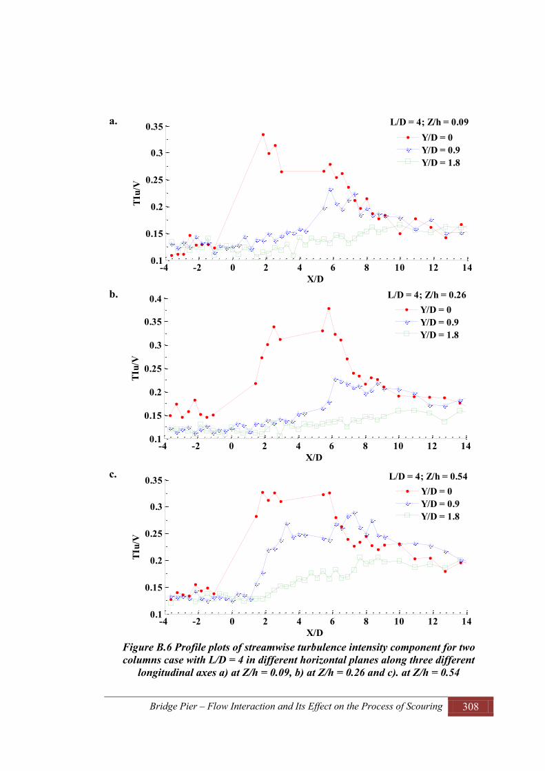
Bridge Pier – Flow Interaction and Its Effect on the Process of Scouring 308
a.
b.
c.
Figure B.6 Profile plots of streamwise turbulence intensity component for two columns case with L/D = 4 in different horizontal planes along three different
longitudinal axes a) at Z/h = 0.09, b) at Z/h = 0.26 and c). at Z/h = 0.54
-4 -2 0 2 4 6 8 10 12 140.1
0.15
0.2
0.25
0.3
0.35
X/D
TIu/
VL/D = 4; Z/h = 0.09
Y/D = 0Y/D = 0.9Y/D = 1.8
-4 -2 0 2 4 6 8 10 12 140.1
0.15
0.2
0.25
0.3
0.35
0.4
X/D
TIu/
V
L/D = 4; Z/h = 0.26
Y/D = 0Y/D = 0.9Y/D = 1.8
-4 -2 0 2 4 6 8 10 12 140.1
0.15
0.2
0.25
0.3
0.35
X/D
TIu/
V
L/D = 4; Z/h = 0.54
Y/D = 0Y/D = 0.9Y/D = 1.8

Bridge Pier – Flow Interaction and Its Effect on the Process of Scouring 309
a.
b.
c.
Figure B.7 Profile plots of streamwise turbulence intensity component for two columns case with L/D = 6 in different horizontal planes along three different
longitudinal axes a) at Z/h = 0.09, b) at Z/h = 0.26 and c). at Z/h = 0.54
-4 -2 0 2 4 6 8 10 12 140.05
0.1
0.15
0.2
0.25
0.3
0.35
X/D
TIu/
V
L/D = 6; Z/h = 0.09
Y/D = 0Y/D = 0.9Y/D = 1.8
-4 -2 0 2 4 6 8 10 12 140.05
0.1
0.15
0.2
0.25
0.3
0.35
X/D
TIu/
V
L/D = 6; Z/h = 0.26
Y/D = 0Y/D = 0.9Y/D = 1.8
-4 -2 0 2 4 6 8 10 12 140.05
0.1
0.15
0.2
0.25
0.3
0.35
X/D
TIu/
V
L/D = 6; Z/h = 0.54
Y/D = 0Y/D = 0.9Y/D = 1.8
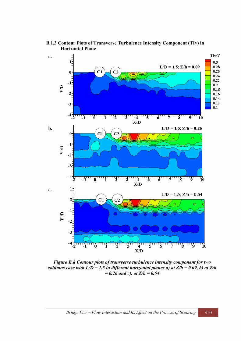
Bridge Pier – Flow Interaction and Its Effect on the Process of Scouring 310
B.1.3 Contour Plots of Transverse Turbulence Intensity Component (TIv) in Horizontal Plane
a.
b.
c.
Figure B.8 Contour plots of transverse turbulence intensity component for two columns case with L/D = 1.5 in different horizontal planes a) at Z/h = 0.09, b) at Z/h
= 0.26 and c). at Z/h = 0.54
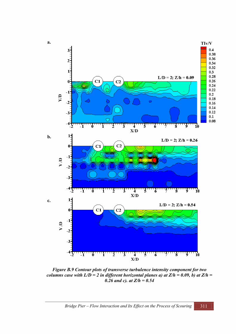
Bridge Pier – Flow Interaction and Its Effect on the Process of Scouring 311
a.
b.
c.
Figure B.9 Contour plots of transverse turbulence intensity component for two columns case with L/D = 2 in different horizontal planes a) at Z/h = 0.09, b) at Z/h =
0.26 and c). at Z/h = 0.54
TIv/V

Bridge Pier – Flow Interaction and Its Effect on the Process of Scouring 312
a.
b.
c.
Figure B.10 Contour plots of transverse turbulence intensity component for two columns case with L/D = 4 in different horizontal planes a) at Z/h = 0.09, b) at Z/h =
0.26 and c). at Z/h = 0.54
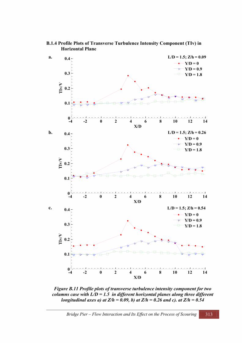
Bridge Pier – Flow Interaction and Its Effect on the Process of Scouring 313
B.1.4 Profile Plots of Transverse Turbulence Intensity Component (TIv) in Horizontal Plane
a.
b.
c.
Figure B.11 Profile plots of transverse turbulence intensity component for two columns case with L/D = 1.5 in different horizontal planes along three different
longitudinal axes a) at Z/h = 0.09, b) at Z/h = 0.26 and c). at Z/h = 0.54
-4 -2 0 2 4 6 8 10 12 140
0.1
0.2
0.3
0.4
X/D
TIv/
VL/D = 1.5; Z/h = 0.09
Y/D = 0Y/D = 0.9Y/D = 1.8
-4 -2 0 2 4 6 8 10 12 140
0.1
0.2
0.3
0.4
X/D
TIv/
V
L/D = 1.5; Z/h = 0.26
Y/D = 0Y/D = 0.9Y/D = 1.8
-4 -2 0 2 4 6 8 10 12 140
0.1
0.2
0.3
0.4
X/D
TIv/
V
L/D = 1.5; Z/h = 0.54
Y/D = 0Y/D = 0.9Y/D = 1.8

Bridge Pier – Flow Interaction and Its Effect on the Process of Scouring 314
a.
b.
c.
Figure B.12 Profile plots of transverse turbulence intensity component for two columns case with L/D = 2 in different horizontal planes along three different
longitudinal axes a) at Z/h = 0.09, b) at Z/h = 0.26 and c). at Z/h = 0.54
-4 -2 0 2 4 6 8 10 12 140
0.1
0.2
0.3
0.4
X/D
TIv/
V
L/D = 2; Z/h = 0.09
Y/D = 0Y/D = 0.9Y/D = 1.8
-4 -2 0 2 4 6 8 10 12 140
0.1
0.2
0.3
0.4
X/D
TIv/
V
L/D = 2; Z/h = 0.26
Y/D = 0Y/D = 0.9Y/D = 1.8
-4 -2 0 2 4 6 8 10 12 140
0.1
0.2
0.3
0.4
X/D
TIv/
V
L/D = 2; Z/h = 0.54
Y/D = 0Y/D = 0.9Y/D = 1.8

Bridge Pier – Flow Interaction and Its Effect on the Process of Scouring 315
a.
b.
c.
Figure B.13 Profile plots of transverse turbulence intensity component for two columns case with L/D = 4 in different horizontal planes along three different
longitudinal axes a) at Z/h = 0.09, b) at Z/h = 0.26 and c). at Z/h = 0.54
-4 -2 0 2 4 6 8 10 12 140
0.1
0.2
0.3
0.4
0.5
0.6
X/D
TIv/
V
L/D = 4; Z/h = 0.09
Y/D = 0Y/D = 0.9Y/D = 1.8
-4 -2 0 2 4 6 8 10 12 140
0.1
0.2
0.3
0.4
0.5
0.6
X/D
TIv/
V
L/D = 4; Z/h = 0.26
Y/D = 0Y/D = 0.9Y/D = 1.8
-4 -2 0 2 4 6 8 10 12 140
0.1
0.2
0.3
0.4
0.5
0.6
X/D
TIv/
V
L/D = 4; Z/h = 0.54
Y/D = 0Y/D = 0.9Y/D = 1.8

Bridge Pier – Flow Interaction and Its Effect on the Process of Scouring 316
a.
b.
c.
Figure B.14 Profile plots of transverse turbulence intensity component for two columns case with L/D = 6 in different horizontal planes along three different
longitudinal axes a) at Z/h = 0.09, b) at Z/h = 0.26 and c). at Z/h = 0.54
-4 -2 0 2 4 6 8 10 12 140
0.2
0.4
0.6
0.8
X/D
TIv/
V
L/D = 6; Z/h = 0.09
Y/D = 0Y/D = 0.9Y/D = 1.8
-4 -2 0 2 4 6 8 10 12 140
0.2
0.4
0.6
0.8
X/D
TIv/
V
L/D = 6; Z/h = 0.26
Y/D = 0Y/D = 0.9Y/D = 1.8
-4 -2 0 2 4 6 8 10 12 140
0.2
0.4
0.6
0.8
X/D
TIv/
V
L/D = 6; Z/h = 0.54
Y/D = 0Y/D = 0.9Y/D = 1.8

Bridge Pier – Flow Interaction and Its Effect on the Process of Scouring 317
B.1.5 Contour Plots of Vertical Turbulence Intensity Component (TIw) in Horizontal Plane
a.
b.
c.
Figure B.15 Contour plots of vertical turbulence intensity component for two columns case with L/D = 1.5 in different horizontal planes a) at Z/h = 0.09, b) at Z/h
= 0.26 and c). at Z/h = 0.54
T

Bridge Pier – Flow Interaction and Its Effect on the Process of Scouring 318
a.
b.
c.
Figure B.16 Contour plots of vertical turbulence intensity component for two columns case with L/D = 2 in different horizontal planes a) at Z/h = 0.09, b) at Z/h =
0.26 and c). at Z/h = 0.54
TIw/V
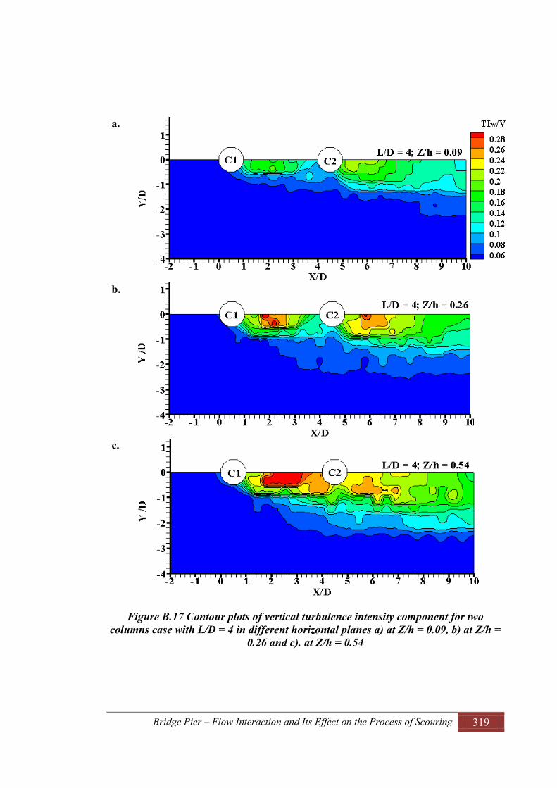
Bridge Pier – Flow Interaction and Its Effect on the Process of Scouring 319
a.
b.
c.
Figure B.17 Contour plots of vertical turbulence intensity component for two columns case with L/D = 4 in different horizontal planes a) at Z/h = 0.09, b) at Z/h =
0.26 and c). at Z/h = 0.54

Bridge Pier – Flow Interaction and Its Effect on the Process of Scouring 320
B.1.6 Profile Plots of Vertical Turbulence Intensity Component (TIw) in Horizontal Plane
a.
b.
c.
Figure B.18 Profile plots of vertical turbulence intensity component for two columns case with L/D = 1.5 in different horizontal planes along three different longitudinal
axes a) at Z/h = 0.09, b) at Z/h = 0.26 and c). at Z/h = 0.54
-4 -2 0 2 4 6 8 10 12 140
0.05
0.1
0.15
0.2
X/D
TIw
/VL/D = 1.5; Z/h = 0.09
Y/D = 0Y/D = 0.9Y/D = 1.8
-4 -2 0 2 4 6 8 10 12 140
0.05
0.1
0.15
0.2
X/D
TIw
/V
L/D = 1.5; Z/h = 0.26
Y/D = 0Y/D = 0.9Y/D = 1.8
-4 -2 0 2 4 6 8 10 12 140
0.05
0.1
0.15
0.2
X/D
TIw
/V
L/D = 1.5; Z/h = 0.54
Y/D = 0Y/D = 0.9Y/D = 1.8

Bridge Pier – Flow Interaction and Its Effect on the Process of Scouring 321
a.
b.
c.
Figure B.19 Profile plots of vertical turbulence intensity component for two columns case with L/D = 2 in different horizontal planes along three different longitudinal
axes a) at Z/h = 0.09, b) at Z/h = 0.26 and c). at Z/h = 0.54
-4 -2 0 2 4 6 8 10 12 140
0.05
0.1
0.15
0.2
0.25
X/D
TIw
/V
L/D = 2; Z/h = 0.09
Y/D = 0Y/D = 0.9Y/D = 1.8
-4 -2 0 2 4 6 8 10 12 140
0.05
0.1
0.15
0.2
0.25
X/D
TIw
/V
L/D = 2; Z/h = 0.26
Y/D = 0Y/D = 0.9Y/D = 1.8
-4 -2 0 2 4 6 8 10 12 140
0.05
0.1
0.15
0.2
0.25
X/D
TIw
/V
L/D = 2; Z/h = 0.54
Y/D = 0Y/D = 0.9Y/D = 1.8

Bridge Pier – Flow Interaction and Its Effect on the Process of Scouring 322
a.
b.
c.
Figure B.20 Profile plots of vertical turbulence intensity component for two columns case with L/D = 4 in different horizontal planes along three different longitudinal
axes a) at Z/h = 0.09, b) at Z/h = 0.26 and c). at Z/h = 0.54
-4 -2 0 2 4 6 8 10 12 140
0.1
0.2
0.3
0.4
X/D
TIw
/V
L/D = 4; Z/h = 0.09
Y/D = 0Y/D = 0.9Y/D = 1.8
-4 -2 0 2 4 6 8 10 12 140
0.1
0.2
0.3
0.4
X/D
TIw
/V
L/D = 4; Z/h = 0.26
Y/D = 0Y/D = 0.9Y/D = 1.8
-4 -2 0 2 4 6 8 10 12 140
0.1
0.2
0.3
0.4
X/D
TIw
/V
L/D = 4; Z/h = 0.54
Y/D = 0Y/D = 0.9Y/D = 1.8
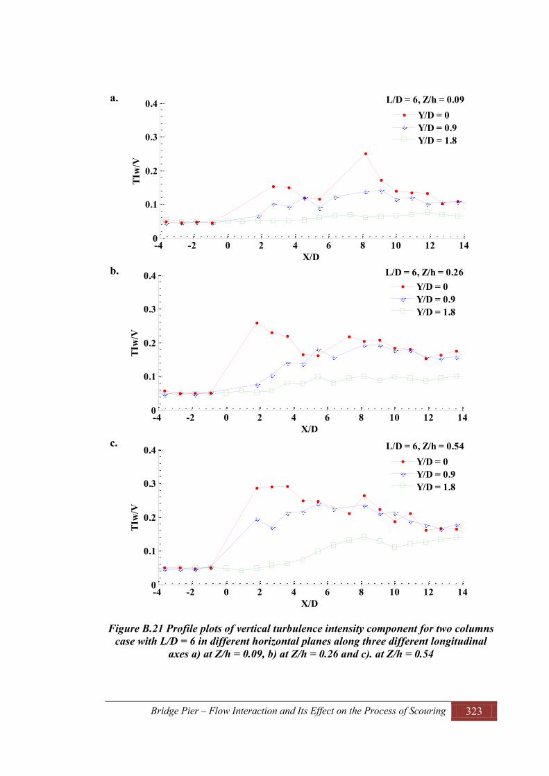
Bridge Pier – Flow Interaction and Its Effect on the Process of Scouring 323
a.
b.
c.
Figure B.21 Profile plots of vertical turbulence intensity component for two columns case with L/D = 6 in different horizontal planes along three different longitudinal
axes a) at Z/h = 0.09, b) at Z/h = 0.26 and c). at Z/h = 0.54
-4 -2 0 2 4 6 8 10 12 140
0.1
0.2
0.3
0.4
X/D
TIw
/V
L/D = 6, Z/h = 0.09
Y/D = 0Y/D = 0.9Y/D = 1.8
-4 -2 0 2 4 6 8 10 12 140
0.1
0.2
0.3
0.4
X/D
TIw
/V
L/D = 6, Z/h = 0.26
Y/D = 0Y/D = 0.9Y/D = 1.8
-4 -2 0 2 4 6 8 10 12 140
0.1
0.2
0.3
0.4
X/D
TIw
/V
L/D = 6, Z/h = 0.54
Y/D = 0Y/D = 0.9Y/D = 1.8

Bridge Pier – Flow Interaction and Its Effect on the Process of Scouring 324
B.2 Plots of Turbulence Intensity in Vertical Plane
B.2.1 Contour Plots of Stream-wise Turbulence Intensity Component (TIu) in Vertical Plane
a.
b.
Figure B.22 Contour plots of streamwise turbulence intensity component for two columns case with L/D = 1 in different vertical planes a) at Y/D = 0, and b) at Y/D =
1.25
TIu/VC1 L/D = 1; Y/D = 0C2
TIu/VC1 C2

Bridge Pier – Flow Interaction and Its Effect on the Process of Scouring 325
a.
b.
Figure B.23 Contour plots of streamwise turbulence intensity component for two
columns case with L/D = 2 in different vertical planes a) at Y/D = 0, and b) at Y/D = 1.25
TIu/VC1 L/D = 2; Y/D = 0C2
TIu/VC1 L/D = 2; Y/D = 1.25C2

Bridge Pier – Flow Interaction and Its Effect on the Process of Scouring 326
a.
b.
Figure B.24 Contour plots of streamwise turbulence intensity component for two
columns case with L/D = 4 in different vertical planes a) at Y/D = 0, and b) at Y/D = 1.25
TIu/VC1 L/D = 4; Y/D = 0C2
TIu/VC1 L/D = 4; Y/D = 1.25C2
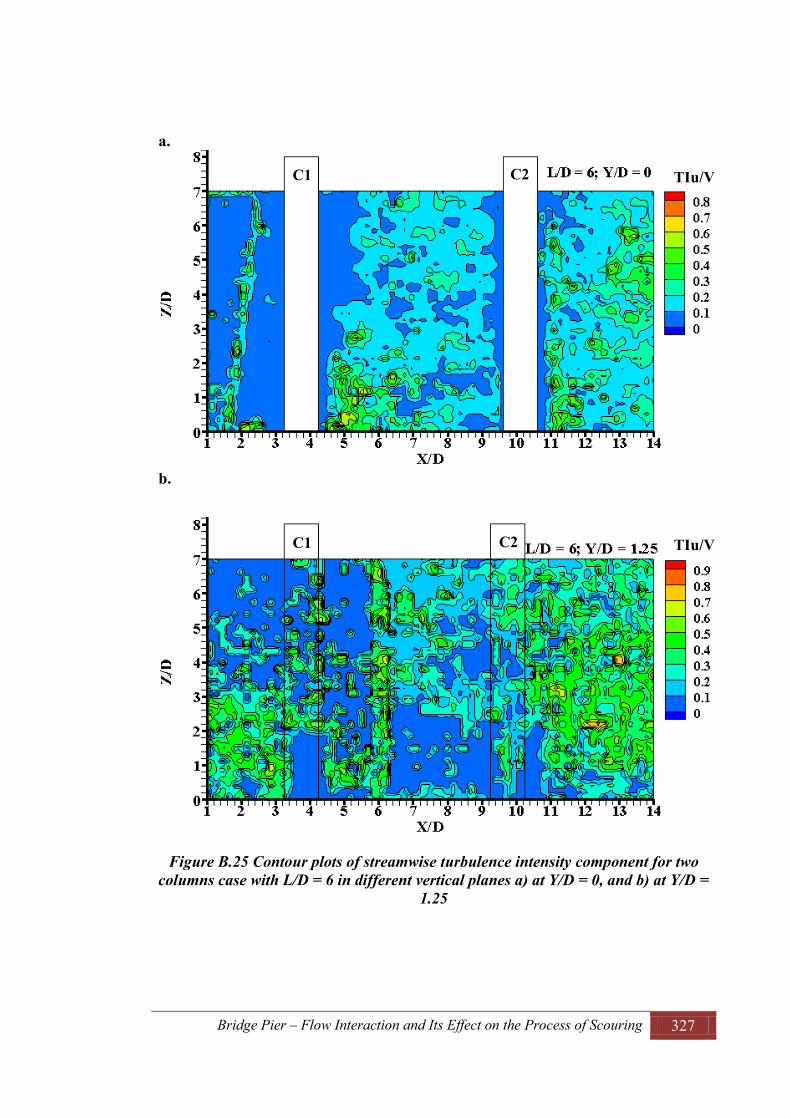
Bridge Pier – Flow Interaction and Its Effect on the Process of Scouring 327
a.
b.
Figure B.25 Contour plots of streamwise turbulence intensity component for two columns case with L/D = 6 in different vertical planes a) at Y/D = 0, and b) at Y/D =
1.25
TIu/VC1 C2
TIu/VC1 C2

Bridge Pier – Flow Interaction and Its Effect on the Process of Scouring 328
B.2.2 Contour Plots of Vertical Component of Turbulence Intensity (TIw) in Vertical Plane
a.
b.
Figure B.26 Contour plots of vertical turbulence intensity component for two columns case with L/D = 1 in different vertical planes a) at Y/D = 0, and b) at Y/D =
1.25
TIw/VC1 L/D = 1; Y/D = 0C2
TIw/VC1 L/D = 1; Y/D = 1.25C2

Bridge Pier – Flow Interaction and Its Effect on the Process of Scouring 329
a.
b.
Figure B.27 Contour plots of vertical turbulence intensity component for two columns case with L/D = 2 in different vertical planes a) at Y/D = 0, and b) at Y/D =
1.25
TIw/VC1 L/D = 2; Y/D = 0C2
TIw/VC1 L/D = 2; Y/D = 1.25C2

Bridge Pier – Flow Interaction and Its Effect on the Process of Scouring 330
a.
b.
Figure B.28 Contour plots of vertical turbulence intensity component for two columns case with L/D = 4 in different vertical planes a) at Y/D = 0, and b) at Y/D =
1.25
TIw/VC1 L/D = 4; Y/D = 0C2
TIw/VC1 L/D = 4; Y/D = 1.25C2

Bridge Pier – Flow Interaction and Its Effect on the Process of Scouring 331
a.
b.
Figure B.29 Contour plots of vertical turbulence intensity component for two columns case with L/D = 6 in different vertical planes a) at Y/D = 0, and b) at Y/D =
1.25
TIw/VC1 L/D = 6; Y/D = 0C2
TIw/VC1 C2

Bridge Pier – Flow Interaction and Its Effect on the Process of Scouring 332
B.2.3 Profile Plots of Streamwise Turbulence Intensity Component (TIu) in Vertical Plane
a. b.
Figure B.30 Profile plots of streamwise turbulence intensity component for two columns with L/D = 1 in a vertical plane at axis of symmetry a) upstream side; b)
downstream side
0 0.5 10
1
2
3
4
5
6
7
TIu/V2
Z/D
US1US2
0 0.5 10
1
2
3
4
5
6
7
TIu/V2
Z/D
DS1DS2DS4
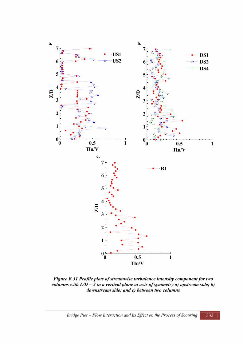
Bridge Pier – Flow Interaction and Its Effect on the Process of Scouring 333
a. b.
c.
Figure B.31 Profile plots of streamwise turbulence intensity component for two columns with L/D = 2 in a vertical plane at axis of symmetry a) upstream side; b)
downstream side; and c) between two columns
0 0.5 10
1
2
3
4
5
6
7
TIu/V
Z/D
US1US2
0 0.5 10
1
2
3
4
5
6
7
TIu/V
Z/D
DS1DS2DS4
0 0.5 10
1
2
3
4
5
6
7
TIu/V
Z/D
B1
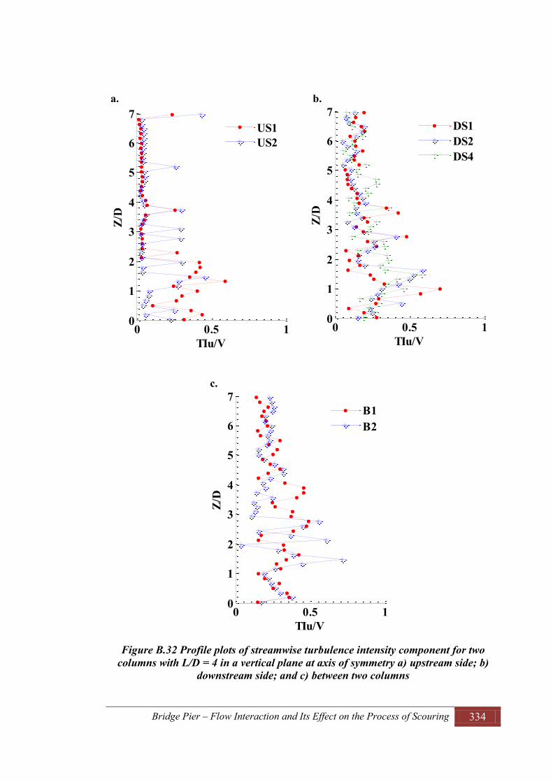
Bridge Pier – Flow Interaction and Its Effect on the Process of Scouring 334
a. b.
c.
Figure B.32 Profile plots of streamwise turbulence intensity component for two columns with L/D = 4 in a vertical plane at axis of symmetry a) upstream side; b)
downstream side; and c) between two columns
0 0.5 10
1
2
3
4
5
6
7
TIu/V
Z/D
US1US2
0 0.5 10
1
2
3
4
5
6
7
TIu/V
Z/D
DS1DS2DS4
0 0.5 10
1
2
3
4
5
6
7
TIu/V
Z/D
B1B2

Bridge Pier – Flow Interaction and Its Effect on the Process of Scouring 335
a. b.
c.
Figure B.33 Profile plots of streamwise turbulence intensity component for two columns with L/D = 6 in a vertical plane at axis of symmetry a) upstream side; b)
downstream side; and c) between two columns
0 0.5 10
1
2
3
4
5
6
7
TIu/V
Z/D
US1US2
0 0.5 10
1
2
3
4
5
6
7
TIu/V
Z/D
DS1DS2DS4
0 0.2 0.4 0.60
1
2
3
4
5
6
7
TIu/V
Z/D
B1B2B3B4

Bridge Pier – Flow Interaction and Its Effect on the Process of Scouring 336
B.2.4 Distribution of Vertical Turbulence Intensity Component (TIw) in Vertical Plane
a. b.
Figure B.34 Profile plots of vertical turbulence intensity component for two columns with L/D = 1 in a vertical plane at axis of symmetry a) upstream side; b) downstream
side
0 0.2 0.40
1
2
3
4
5
6
7
TIw/V
Z/D
US1US2
0 0.2 0.40
1
2
3
4
5
6
7
TIw/V
Z/D
DS1DS2DS4

Bridge Pier – Flow Interaction and Its Effect on the Process of Scouring 337
a. b.
c.
Figure B.35 Profile plots of vertical turbulence intensity component for two columns with L/D = 2 in a vertical plane at axis of symmetry a) upstream side; b) downstream
side; and c) between two columns
0 0.2 0.40
1
2
3
4
5
6
7
TIw/V
Z/D
US1US2
0 0.2 0.40
1
2
3
4
5
6
7
TIw/V
Z/D
DS1DS2DS4
0 0.5 10
1
2
3
4
5
6
7
TIw/V
Z/D
B1
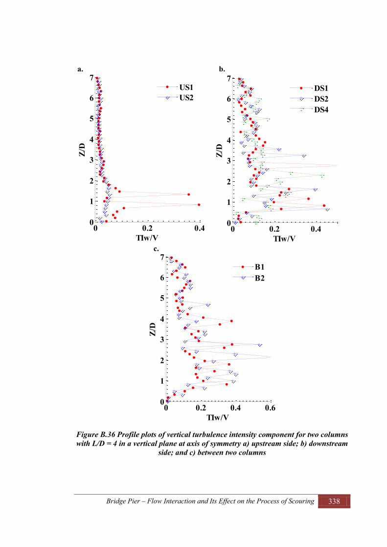
Bridge Pier – Flow Interaction and Its Effect on the Process of Scouring 338
a. b.
c.
Figure B.36 Profile plots of vertical turbulence intensity component for two columns with L/D = 4 in a vertical plane at axis of symmetry a) upstream side; b) downstream
side; and c) between two columns
0 0.2 0.40
1
2
3
4
5
6
7
TIw/V
Z/D
US1US2
0 0.2 0.40
1
2
3
4
5
6
7
TIw/V
Z/D
DS1DS2DS4
0 0.2 0.4 0.60
1
2
3
4
5
6
7
TIw/V
Z/D
B1B2

Bridge Pier – Flow Interaction and Its Effect on the Process of Scouring 339
a. b.
c.
Figure B.37 Profile plots of vertical turbulence intensity component for two columns with L/D = 6 in a vertical plane at axis of symmetry a) upstream side; b) downstream
side; and c) between two columns
0 0.1 0.20
1
2
3
4
5
6
7
TIw/V
Z/D
US2
0 0.2 0.4 0.60
1
2
3
4
5
6
7
TIw/V
Z/D
DS1DS2DS4
0 0.2 0.40
1
2
3
4
5
6
7
TIw/V
Z/D
B1B2B3B4

Bridge Pier – Flow Interaction and Its Effect on the Process of Scouring 340
B.3 Table of Results on Turbulence Intensity Components Table B. 1 Maximum and minimum values of streamwise turbulence intensity components
Test No.
L/D Z/h Y/D TIumax/V X/D TIumin/V X/D
1 0
0.09 0 0.31 2 0.12 -2 0.9 0.22 4.5 0.1 0 1.8 0.17 4.5 0.1 1
0.26 0 0.38 2 0.11 -4 0.9 0.29 2.5 0.11 -1 1.8 0.16 6.5 0.1 1
0.54 0 0.37 2 0.11 -1 0.9 0.32 2.5 0.11 0 1.8 0.18 6 0.11 0
2 1.5
0.09 0 0.25 4 0.12 -2 0.9 0.17 7 0.12 -2 1.8 0.15 7 0.11 0
0.26 0 0.27 4 0.15 -2 0.9 0.19 6.5 0.13 -1 1.8 0.15 0.15
0.54 0 0.27 3.5 0.15 -4 0.9 0.2 6.5 0.1 -2 1.8 0.14 3.5 0.1 0
3 2
0.09 0 0.28 1 0.13 -3 0.9 0.22 4 0.13 -4 1.8 0.15 -1.5 0.13 -4
0.26 0 0.28 4.5 0.1 -4 0.9 0.16 7 0.12 -3 1.8 0.14 6.5 0.08 2
0.54 0 0.26 4.5 0.1 -3 0.9 0.22 5.5 0.1 -1 1.8 0.12 8 0.08 -2
4 3
0.09 0 0.32 4 0.13 -1 0.9 0.24 5 0.12 2 1.8 0.18 11 0.12 2.5
0.26 0 0.33 2.5 0.12 -2 0.9 0.22 7 0.11 -1 1.8 0.16 6 0.11 0
0.54 0 0.29 4 0.12 -1 0.9 0.25 4 0.12 -1 1.8 0.17 9 0.11 0
5 4 0.09 0 0.33 2 0.1 -3 0.9 0.23 6 0.12 -1 1.8 0.16 8 0.1 4
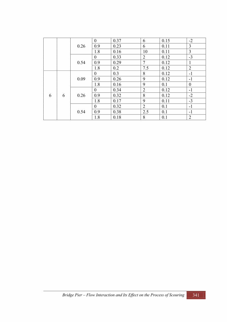
Bridge Pier – Flow Interaction and Its Effect on the Process of Scouring 341
0.26 0 0.37 6 0.15 -2 0.9 0.23 6 0.11 3 1.8 0.16 10 0.11 3
0.54 0 0.33 2 0.12 -3 0.9 0.29 7 0.12 1 1.8 0.2 7.5 0.12 2
6 6
0.09 0 0.3 8 0.12 -1 0.9 0.26 9 0.12 -1 1.8 0.16 9 0.1 0
0.26 0 0.34 2 0.12 -1 0.9 0.32 8 0.12 -2 1.8 0.17 9 0.11 -3
0.54 0 0.32 2 0.1 -1 0.9 0.38 2.5 0.1 -1 1.8 0.18 8 0.1 2

Bridge Pier – Flow Interaction and Its Effect on the Process of Scouring 342
Table B. 2 Maximum and minimum values of transverse turbulence intensity components
Test No.
L/D Z/h Y/D TIvmax/V X/D TIvmin/V X/D
1 0
0.09 0 0.27 2 0.1 -2 0.9 0.2 2 0.09 -1 1.8 0.16 2 0.09 1
0.26 0 0.58 2 0.08 -2 0.9 0.33 3.5 0.08 -1 1.8 0.14 6.5 0.08 0
0.54 0 0.64 3 0.08 -1 0.9 0.37 3.5 0.08 0 1.8 0.2 6.5 0.08 0
2 1.5
0.09 0 0.29 3.5 0.1 -1 0.9 0.16 7 0.1 -1 1.8 0.13 12 0.1 6.5
0.26 0 0.32 3.5 0.1 -3 0.9 0.19 7 0.1 -2 1.8 0.14 9 0.1 5.5
0.54 0 0.33 3.5 0.16 -1 0.9 0.2 8 0.1 -1 1.8 0.12 2 0.1 0
3 2
0.09 0 0.28 1 0.1 -3 0.9 0.2 1.5 0.1 -2 1.8 0.12 8 0.1 5.5
0.26 0 0.34 4.5 0.1 -1 0.9 0.16 7 0.1 -1 1.8 0.12 4.5 0.08 3
0.54 0 0.33 4.5 0.07 -1 0.9 0.18 7 0.07 0 1.8 0.11 11 0.07 0
4 3
0.09 0 0.33 5 0.1 -2 0.9 0.16 7 0.1 3.5 1.8 0.15 11 0.1 3.5
0.26 0 0.38 5.5 0.1 -1.5 0.9 0.23 6.9 0.1 -1.5 1.8 0.13 12 0.1 2
0.54 0 0.42 5 0.1 -1 0.9 0.24 6.5 0.1 -1 1.8 0.16 9 0.1 -1
5 4 0.09
0 0.35 6 0.1 -1 0.9 0.21 9 0.1 0 1.8 0.12 11 0.1 3
0.26 0 0.45 6 0.11 -2 0.9 0.25 8 0.1 0

Bridge Pier – Flow Interaction and Its Effect on the Process of Scouring 343
1.8 0.15 12 0.1 3
0.54 0 0.52 3 0.11 -1 0.9 0.3 3.5 0.12 1.5 1.8 0.2 5.5 0.12 1.5
6 6
0.09 0 0.46 3 0.1 -1 0.9 0.28 4.5 0.1 -1 1.8 0.15 10 0.1 -1
0.26 0 0.64 2 0.1 -1 0.9 0.32 4.5 0.1 -2 1.8 0.16 7.5 0.1 -2
0.54
0 0.48 2 0.1 -1 0.9 0.36 3 0.1 -1 1.8 0.22 6.5 0.1 -1

Bridge Pier – Flow Interaction and Its Effect on the Process of Scouring 344
Table B. 3 Maximum and minimum values of vertical turbulence intensity components
Test No.
L/D Z/h Y/D TIwmax/V X/D TIwmin/V X/D
1 0
0.09 0 0.18 2 0.05 -1 0.9 0.07 3.5 0.05 -1 1.8 0.06 2 0.05 -1
0.26 0 0.3 2 0.05 -1 0.9 0.2 3.5 0.05 -1 1.8 0.12 6.5 0.05 0
0.54 0 0.3 2 0.05 -1 0.9 0.2 3.5 0.05 0 1.8 0.15 8 0.05 0
2 1.5
0.09 0 0.17 3.5 0.05 -1 0.9 0.08 7 0.05 -1 1.8 0.07 12 0.05 5.5
0.26 0 0.32 4 0.1 -2 0.9 0.2 5.5 0.1 -2 1.8 0.14 9 0.1 -2
0.54 0 0.32 4 0.16 -1 0.9 0.2 5.5 0.1 -1 1.8 0.12 2 0.1 -1
3 2
0.09 0 0.28 1 0.1 -2 0.9 0.2 1.5 0.1 -2 1.8 0.12 8 0.1 -2
0.26 0 0.34 4 0.08 -1 0.9 0.16 7 0.08 -1 1.8 0.12 5 0.07 3
0.54 0 0.33 5 0.07 -1 0.9 0.18 7 0.07 0 1.8 0.11 11 0.07 0
4 3
0.09 0 0.2 5 0.05 -2 0.9 0.1 7 0.05 -2 1.8 0.08 11 0.05 -2
0.26 0 0.22 5.5 0.05 -1 0.9 0.13 8 0.05 -1 1.8 0.09 11 0.05 0
0.54 0 0.22 4.5 0.05 -1 0.9 0.16 6.5 0.05 0 1.8 0.11 12 0.05 0
5 4 0.09
0 0.35 2 0.1 -1 0.9 0.2 9 0.1 0 1.8 0.15 11 0.1 3
0.26 0 0.45 6 0.11 -1 0.9 0.25 8 0.1 3
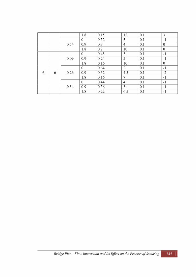
Bridge Pier – Flow Interaction and Its Effect on the Process of Scouring 345
1.8 0.15 12 0.1 3
0.54 0 0.52 3 0.1 -1 0.9 0.3 4 0.1 0 1.8 0.2 10 0.1 0
6 6
0.09 0 0.45 3 0.1 -1 0.9 0.24 5 0.1 -1 1.8 0.16 10 0.1 0
0.26 0 0.64 2 0.1 -1 0.9 0.32 4.5 0.1 -2 1.8 0.16 7 0.1 -1
0.54 0 0.44 4 0.1 -1 0.9 0.36 3 0.1 -1 1.8 0.22 6.5 0.1 -1

Bridge Pier – Flow Interaction and Its Effect on the Process of Scouring 346
APPENDIX-C: PLOTS FOR TURBULENT KINETIC ENERGY
C.1 Plots of Turbulent Kinetic Energy in Horizontal Plane
C.1.1 Contour Plots of Turbulent Kinetic Energy in Horizontal Plane a.
b.
c.
Figure C.1 Contour plots of turbulent kinetic energy for two columns case with L/D = 1.5 in different horizontal planes a) at Z/h = 0.09, b) at Z/h = 0.26 and c). at Z/h =
0.54
TKE/V2

Bridge Pier – Flow Interaction and Its Effect on the Process of Scouring 347
a.
b.
c.
Figure C.2 Contour plots of turbulent kinetic energy for two columns case with L/D = 2 in different horizontal planes a) at Z/h = 0.09, b) at Z/h = 0.26 and c). at Z/h = 0.54
TKE/V2

Bridge Pier – Flow Interaction and Its Effect on the Process of Scouring 348
a.
b.
c.
Figure C.3 Contour plots of turbulent kinetic energy for two columns case with L/D = 4 in different horizontal planes a) at Z/h = 0.09, b) at Z/h = 0.26 and c). at Z/h = 0.54
TKE/V2
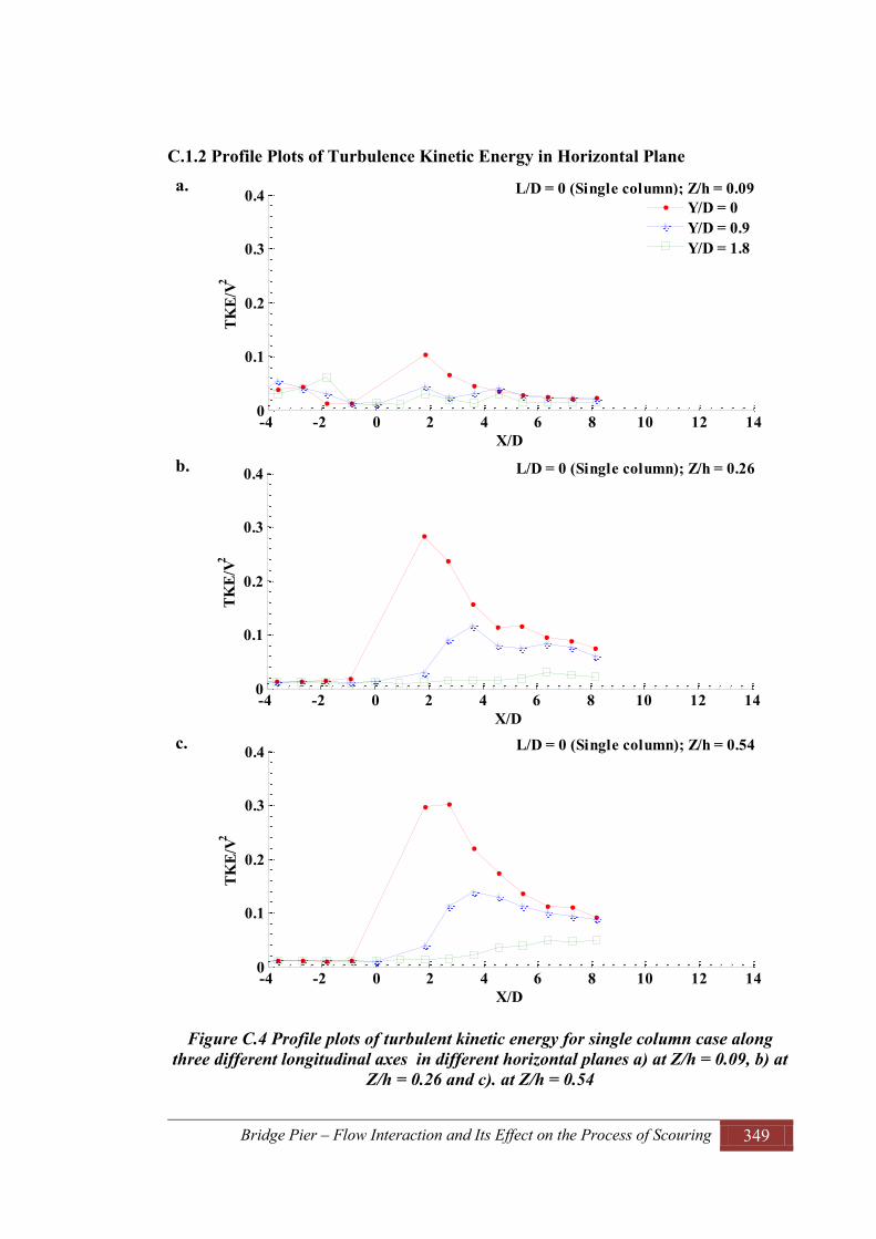
Bridge Pier – Flow Interaction and Its Effect on the Process of Scouring 349
C.1.2 Profile Plots of Turbulence Kinetic Energy in Horizontal Plane a.
b.
c.
Figure C.4 Profile plots of turbulent kinetic energy for single column case along three different longitudinal axes in different horizontal planes a) at Z/h = 0.09, b) at
Z/h = 0.26 and c). at Z/h = 0.54
-4 -2 0 2 4 6 8 10 12 140
0.1
0.2
0.3
0.4
X/D
TKE/
V2
L/D = 0 (Single column); Z/h = 0.09
Y/D = 0Y/D = 0.9Y/D = 1.8
-4 -2 0 2 4 6 8 10 12 140
0.1
0.2
0.3
0.4
X/D
TKE/
V2
L/D = 0 (Single column); Z/h = 0.26
-4 -2 0 2 4 6 8 10 12 140
0.1
0.2
0.3
0.4
X/D
TKE/
V2
L/D = 0 (Single column); Z/h = 0.54

Bridge Pier – Flow Interaction and Its Effect on the Process of Scouring 350
a.
b.
c.
Figure C.5 Profile plots of turbulent kinetic energy for two columns case with L/D = 1.5 along three different longitudinal axes in different horizontal planes a) at Z/h =
0.09, b) at Z/h = 0.26 and c). at Z/h = 0.54
-4 -2 0 2 4 6 8 10 12 140
0.02
0.04
0.06
0.08
0.1
0.12
X/D
TKE/
V2
L/D = 1.5; Z/h = 0.09
Y/D = 0Y/D = 0.9Y/D = 1.8
-4 -2 0 2 4 6 8 10 12 140
0.02
0.04
0.06
0.08
0.1
0.12
X/D
TKE/
V2
L/D = 1.5; Z/h = 0.26
-4 -2 0 2 4 6 8 10 12 140
0.02
0.04
0.06
0.08
0.1
0.12
X/D
TKE/
V2
L/D = 1.5; Z/h = 0.54

Bridge Pier – Flow Interaction and Its Effect on the Process of Scouring 351
a.
b.
c.
Figure C.6 Profile plots of turbulent kinetic energy for two columns case with L/D = 2 along three different longitudinal axes in different horizontal planes a) at Z/h =
0.09, b) at Z/h = 0.26 and c). at Z/h = 0.54
-4 -2 0 2 4 6 8 10 12 140
0.02
0.04
0.06
0.08
0.1
0.12
X/D
TKE/
V2
Y/D = 2; Z/h = 0.09
Y/D = 0Y/D = 0.9Y/D = 1.8
-4 -2 0 2 4 6 8 10 12 140
0.02
0.04
0.06
0.08
0.1
0.12
X/D
TKE/
V2
Y/D = 2; Z/h = 0.26
-4 -2 0 2 4 6 8 10 12 140
0.02
0.04
0.06
0.08
0.1
0.12
X/D
TKE/
V2
Y/D = 2; Z/h = 0.54
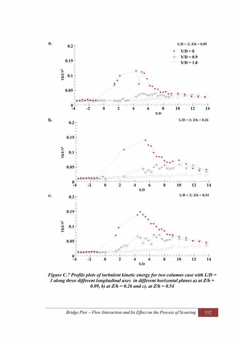
Bridge Pier – Flow Interaction and Its Effect on the Process of Scouring 352
a.
b.
c.
Figure C.7 Profile plots of turbulent kinetic energy for two columns case with L/D = 3 along three different longitudinal axes in different horizontal planes a) at Z/h =
0.09, b) at Z/h = 0.26 and c). at Z/h = 0.54
-4 -2 0 2 4 6 8 10 12 140
0.05
0.1
0.15
0.2
X/D
TKE/
V2
L/D = 3; Z/h = 0.09
Y/D = 0Y/D = 0.9Y/D = 1.8
-4 -2 0 2 4 6 8 10 12 140
0.05
0.1
0.15
0.2
X/D
TKE/
V2
L/D = 3; Z/h = 0.26
-4 -2 0 2 4 6 8 10 12 140
0.05
0.1
0.15
0.2
X/D
TKE/
V2
L/D = 3; Z/h = 0.54

Bridge Pier – Flow Interaction and Its Effect on the Process of Scouring 353
a.
b.
c.
Figure C.8 Profile plots of turbulent kinetic energy for two columns case with L/D = 4 along three different longitudinal axes in different horizontal planes a) at Z/h =
0.09, b) at Z/h = 0.26 and c). at Z/h = 0.54
-4 -2 0 2 4 6 8 10 12 140
0.05
0.1
0.15
0.2
0.25
X/D
TKE/
V2
L/D = 4; Z/h = 0.09
Y/D = 0Y/D = 0.9Y/D = 1.8
-4 -2 0 2 4 6 8 10 12 140
0.05
0.1
0.15
0.2
0.25
X/D
TKE/
V2
L/D = 4; Z/h = 0.26
-4 -2 0 2 4 6 8 10 12 140
0.05
0.1
0.15
0.2
0.25
X/D
TKE/
V2
L/D = 4; Z/h = 0.54

Bridge Pier – Flow Interaction and Its Effect on the Process of Scouring 354
a.
b.
c.
Figure C.9 Profile plots of turbulent kinetic energy for two columns case with L/D = 6 along three different longitudinal axes in different horizontal planes a) at Z/h =
0.09, b) at Z/h = 0.26 and c). at Z/h = 0.54
-4 -2 0 2 4 6 8 10 12 140
0.1
0.2
0.3
0.4
X/D
TKE/
V2
L/D = 6; Z/h = 0.09
Y/D = 0Y/D = 0.9Y/D = 1.8
-4 -2 0 2 4 6 8 10 12 140
0.1
0.2
0.3
0.4
X/D
TKE/
V2
L/D = 6; Z/h = 0.26
-4 -2 0 2 4 6 8 10 12 140
0.1
0.2
0.3
0.4
X/D
TKE/
V2
L/D = 6; Z/h = 0.54

Bridge Pier – Flow Interaction and Its Effect on the Process of Scouring 355
C.2 Plots of Turbulent Kinetic Energy in Vertical Plane
C.2.1 Contour Plots of Turbulent Kinetic Energy in Vertical Plane a.
b.
Figure C.10 Contour plots of turbulent kinetic energy for two columns case with L/D = 1 in different vertical planes a) at Y/D = 0, and b) at Y/D = 1.25
TKE/V2C1 L/D = 1; Y/D = 0C2
TKE/V2C1 L/D = 1; Y/D = 1.25C2
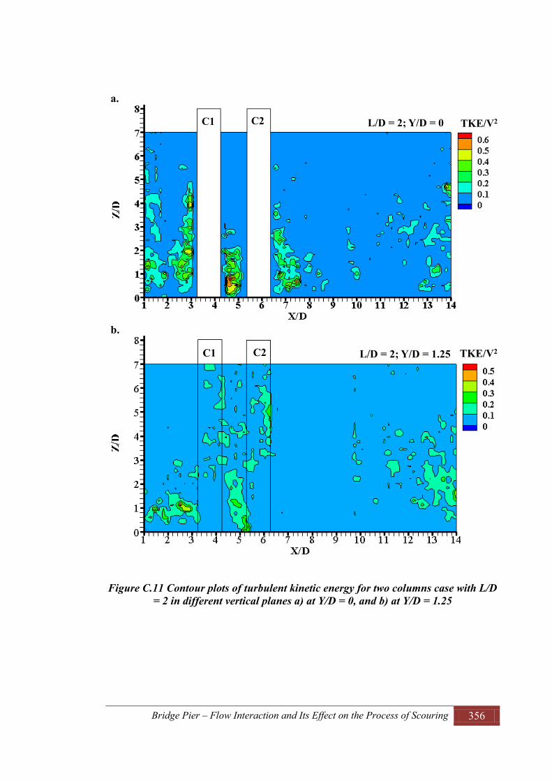
Bridge Pier – Flow Interaction and Its Effect on the Process of Scouring 356
a.
b.
Figure C.11 Contour plots of turbulent kinetic energy for two columns case with L/D = 2 in different vertical planes a) at Y/D = 0, and b) at Y/D = 1.25
TKE/V2C1 L/D = 2; Y/D = 0C2
TKE/V2C1 L/D = 2; Y/D = 1.25C2
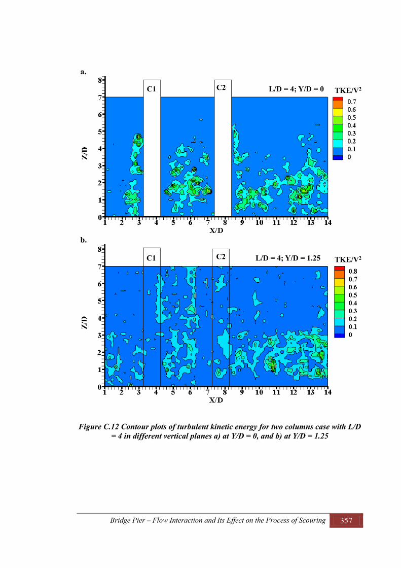
Bridge Pier – Flow Interaction and Its Effect on the Process of Scouring 357
a.
b.
Figure C.12 Contour plots of turbulent kinetic energy for two columns case with L/D = 4 in different vertical planes a) at Y/D = 0, and b) at Y/D = 1.25
TKE/V2C1 L/D = 4; Y/D = 0C2
TKE/V2C1 L/D = 4; Y/D = 1.25C2

Bridge Pier – Flow Interaction and Its Effect on the Process of Scouring 358
a.
b.
Figure C.13 Contour plots of turbulent kinetic energy for two columns case with L/D = 6 in different vertical planes a) at Y/D = 0, and b) at Y/D = 1.25
TKE/V2C1 L/D = 6; Y/D = 0C2
TKE/V2C1 C2
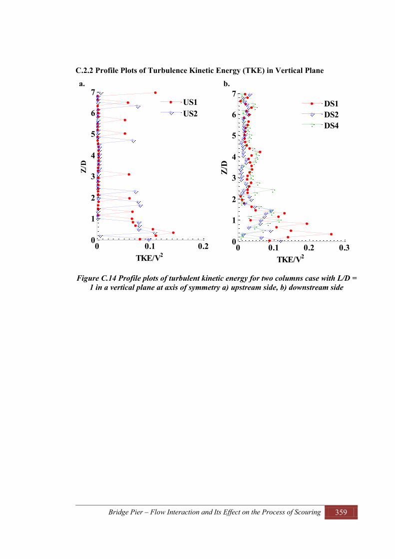
Bridge Pier – Flow Interaction and Its Effect on the Process of Scouring 359
C.2.2 Profile Plots of Turbulence Kinetic Energy (TKE) in Vertical Plane a. b.
Figure C.14 Profile plots of turbulent kinetic energy for two columns case with L/D = 1 in a vertical plane at axis of symmetry a) upstream side, b) downstream side
0 0.1 0.20
1
2
3
4
5
6
7
TKE/V2
Z/D
US1US2
0 0.1 0.2 0.30
1
2
3
4
5
6
7
TKE/V2
Z/D
DS1DS2DS4
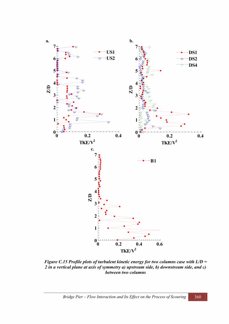
Bridge Pier – Flow Interaction and Its Effect on the Process of Scouring 360
a. b.
c.
Figure C.15 Profile plots of turbulent kinetic energy for two columns case with L/D = 2 in a vertical plane at axis of symmetry a) upstream side, b) downstream side, and c)
between two columns
0 0.2 0.40
1
2
3
4
5
6
7
TKE/V2
Z/D
US1US2
0 0.2 0.40
1
2
3
4
5
6
7
TKE/V2
Z/D
DS1DS2DS4
0 0.2 0.4 0.60
1
2
3
4
5
6
7
TKE/V2
Z/D
B1

Bridge Pier – Flow Interaction and Its Effect on the Process of Scouring 361
a. b.
c.
Figure C.16 Profile plots of turbulent kinetic energy for two columns case with L/D = 4 in a vertical plane at axis of symmetry a) upstream side, b) downstream side, and c)
between two columns
0 0.2 0.40
1
2
3
4
5
6
7
TKE/V2
Z/D
US1US2
0 0.2 0.40
1
2
3
4
5
6
7
TKE/V2
Z/D
DS1DS2DS4
0 0.2 0.40
1
2
3
4
5
6
7
TKE/V2
Z/D
B1B2

Bridge Pier – Flow Interaction and Its Effect on the Process of Scouring 362
a. b.
c.
Figure C.17 Profile plots of turbulent kinetic energy for two columns case with L/D = 6 in a vertical plane at axis of symmetry a) upstream side, b) downstream side, and c)
between two columns
0 0.1 0.20
1
2
3
4
5
6
7
TKE/V2
Z/D
US2
0 0.2 0.40
1
2
3
4
5
6
7
TKE/V2
Z/D
DS1DS2DS4
0 0.1 0.2 0.30
1
2
3
4
5
6
7
TKE/V2
Z/D
B1B2B3B4

Bridge Pier – Flow Interaction and Its Effect on the Process of Scouring 363
C.3 Table of Results on Turbulent Kinetic Energy Table C. 1 Maximum and minimum values of turbulent kinetic energy
Test No.
L/D Z/h Y/D TKE max/V2 X/D TKEmin/V2 X/D
1 0
0.09 0 0.11 2 0.02 -1 0.9 0.05 2 0.02 1 1.8 0.03 2 0.02 1
0.26 0 0.28 2 0.02 -1 0.9 0.12 3.5 0.02 0 1.8 0.03 6.5 0.02 2
0.54 0 0.3 3 0.02 -1 0.9 0.14 4 0.02 0 1.8 0.06 6.5 0.02 3
2 1.5
0.09 0 0.09 4 0.015 -1 0.9 0.035 7.5 0.015 -1 1.8 0.02 11 0.015 3
0.26 0 0.11 4 0.02 -2 0.9 0.04 5.5 0.02 -2 1.8 0.03 13 0.02 5.5
0.54 0 0.11 4 0.03 -1 0.9 0.04 7 0.01 -2 1.8 0.02 4 0.01 0
3 2
0.09 0 0.09 1 0.02 -1 0.9 0.05 4 0.02 -2 1.8 0.02 8 0.015 6
0.26 0 0.12 4.5 0.01 -1 0.9 0.03 7.5 0.01 -1 1.8 0.02 4.5 0.01 2
0.54 0 0.11 4.5 0.01 -1 0.9 0.05 6 0.01 0 1.8 0.02 11 0.01 1
4 3
0.09 0 0.12 4 0.02 -1 0.9 0.04 5 0.02 3 1.8 0.03 11 0.02 3
0.26 0 0.14 5.5 0.02 -1 0.9 0.06 8 0.02 0 1.8 0.03 10 0.02 0
0.54 0 0.15 5 0.02 -1 0.9 0.07 7 0.02 1.5 1.8 0.04 12 0.02 2
5 4 0.09 0 0.13 2 0.01 -1 0.9 0.05 6 0.01 0 1.8 0.025 10 0.01 4
0.26 0 0.22 6 0.025 -1
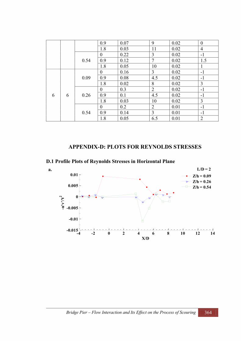
Bridge Pier – Flow Interaction and Its Effect on the Process of Scouring 364
0.9 0.07 9 0.02 0 1.8 0.03 11 0.02 4
0.54 0 0.22 3 0.02 -1 0.9 0.12 7 0.02 1.5 1.8 0.05 10 0.02 1
6 6
0.09 0 0.16 3 0.02 -1 0.9 0.08 4.5 0.02 -1 1.8 0.02 8 0.02 3
0.26 0 0.3 2 0.02 -1 0.9 0.1 4.5 0.02 -1 1.8 0.03 10 0.02 3
0.54 0 0.2 2 0.01 -1 0.9 0.14 3 0.01 -1 1.8 0.05 6.5 0.01 2
APPENDIX-D: PLOTS FOR REYNOLDS STRESSES
D.1 Profile Plots of Reynolds Stresses in Horizontal Plane a.
-4 -2 0 2 4 6 8 10 12 14
-0.015
-0.01
-0.005
0
0.005
0.01
X/D
-u'v
'/V2
L/D = 2
Z/h = 0.09Z/h = 0.26Z/h = 0.54

Bridge Pier – Flow Interaction and Its Effect on the Process of Scouring 365
b.
c.
Figure D.1 Profile plots of Reynolds shear stresses for two columns case with L/D = 2 in different horizontal planes along axix of symmetry a) in u-v plane, b) in u-w plane,
and c) in v-w plane
a.
-4 -2 0 2 4 6 8 10 12 14-0.015
-0.01
-0.005
0
0.005
0.01
X/D
-u'w
'/V2
-4 -2 0 2 4 6 8 10 12 14-0.015
-0.01
-0.005
0
0.005
0.01
X/D
-v'w
'/V2
-4 -2 0 2 4 6 8 10 12 14-0.02
-0.01
0
0.01
0.02
0.03
0.04
X/D
-u'v
'/V2
L/D = 4
Z/h = 0.09Z/h = 0.26Z/h = 0.54

Bridge Pier – Flow Interaction and Its Effect on the Process of Scouring 366
b.
c.
Figure D.2 Profile plots of Reynolds shear stresses for two columns case with L/D = 4 in different horizontal planes along axix of symmetry a) in u-v plane, b) in u-w plane,
and c) in v-w plane
a.
-4 -2 0 2 4 6 8 10 12 14-0.02
-0.01
0
0.01
0.02
0.03
0.04
X/D
-u'w
'/V2
-4 -2 0 2 4 6 8 10 12 14-0.02
-0.01
0
0.01
0.02
0.03
0.04
X/D
-v'w
'/V2
-4 -2 0 2 4 6 8 10 12 14-0.03
-0.02
-0.01
0
0.01
0.02
X/D
-u'v
'/V2
L/D = 6
Z/h = 0.09Z/h = 0.26Z/h = 0.54

Bridge Pier – Flow Interaction and Its Effect on the Process of Scouring 367
b.
c.
Figure D.3 Profile plots of Reynolds shear stresses for two columns case with L/D = 6 in different horizontal planes along axix of symmetry a) in u-v plane, b) in u-w plane,
and c) in v-w plane
-4 -2 0 2 4 6 8 10 12 14-0.03
-0.02
-0.01
0
0.01
0.02
X/D
-u'w
'/V2
-4 -2 0 2 4 6 8 10 12 14-0.03
-0.02
-0.01
0
0.01
0.02
X/D
-v'w
'/V2
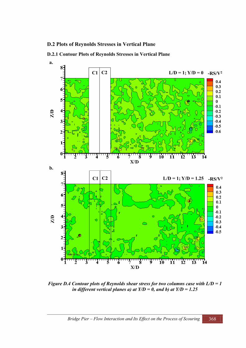
Bridge Pier – Flow Interaction and Its Effect on the Process of Scouring 368
D.2 Plots of Reynolds Stresses in Vertical Plane
D.2.1 Contour Plots of Reynolds Stresses in Vertical Plane a.
b.
Figure D.4 Contour plots of Reynolds shear stress for two columns case with L/D = 1 in different vertical planes a) at Y/D = 0, and b) at Y/D = 1.25
-RS/V2C1 L/D = 1; Y/D = 0C2
-RS/V2C1 L/D = 1; Y/D = 1.25C2

Bridge Pier – Flow Interaction and Its Effect on the Process of Scouring 369
a.
b.
Figure D.5 Contour plots of Reynolds shear stress for two columns case with L/D = 2 in different vertical planes a) at Y/D = 0, and b) at Y/D = 1.25
-RS/V2C1 L/D = 2; Y/D = 0C2
-RS/V2C1 L/D = 2; Y/D = 1.25C2

Bridge Pier – Flow Interaction and Its Effect on the Process of Scouring 370
a.
b.
Figure D.6 Contour plots of Reynolds shear stress for two columns case with L/D = 4 in different vertical planes a) at Y/D = 0, and b) at Y/D = 1.25
-RS/V2C1 L/D = 4; Y/D = 0C2
-RS/V2C1 C2

Bridge Pier – Flow Interaction and Its Effect on the Process of Scouring 371
a.
b.
Figure D.7 Contour plots of Reynolds shear stress for two columns case with L/D = 6 in different vertical planes a) at Y/D = 0, and b) at Y/D = 1.25
-RS/V2C1 C2
-RS/V2C1 C2

Bridge Pier – Flow Interaction and Its Effect on the Process of Scouring 372
D.2.2 Profile Plots of Reynolds Stresses in Vertical Plane a. b.
Figure D.8 Profile plots of Reynolds shear stress for two columns case with L/D = 1 in a vertical plane at axis of symmetry a) upstream side, b) downstream side
-0.05 0 0.050
1
2
3
4
5
6
7
RS/V2
Z/D
US1US2
-0.2 0 0.20
1
2
3
4
5
6
7
RS/V2
Z/D
DS1DS2DS4

Bridge Pier – Flow Interaction and Its Effect on the Process of Scouring 373
a. b.
c.
Figure D.9 Profile plots of Reynolds shear stress for two columns case with L/D = 2 in a vertical plane at axis of symmetry a) upstream side, b) downstream side, and c)
between two columns
-0.2 0 0.20
1
2
3
4
5
6
7
RS/V2
Z/D
US1US2
-0.2 0 0.20
1
2
3
4
5
6
7
RS/V2
Z/D
DS1DS2DS4
-0.5 0 0.50
1
2
3
4
5
6
7
RS/V2
Z/D
B1

Bridge Pier – Flow Interaction and Its Effect on the Process of Scouring 374
a. b.
c.
Figure D.10 Profile plots of Reynolds shear stress for two columns case with L/D = 4 in a vertical plane at axis of symmetry a) upstream side, b) downstream side, and c)
between two columns
-0.2 0 0.20
1
2
3
4
5
6
7
RS/V2
Z/D
US1US2
-0.2 0 0.20
1
2
3
4
5
6
7
RS/V2
Z/D
DS1DS2DS4
-0.5 0 0.50
1
2
3
4
5
6
7
RS/V2
Z/D
B1B2
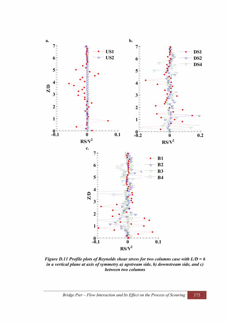
Bridge Pier – Flow Interaction and Its Effect on the Process of Scouring 375
a. b.
c.
Figure D.11 Profile plots of Reynolds shear stress for two columns case with L/D = 6 in a vertical plane at axis of symmetry a) upstream side, b) downstream side, and c)
between two columns
-0.1 0 0.10
1
2
3
4
5
6
7
RS/V2
Z/D
US1US2
-0.2 0 0.20
1
2
3
4
5
6
7
RS/V2
DS1DS2DS4
-0.1 0 0.10
1
2
3
4
5
6
7
RS/V2
Z/D
B1B2B3B4
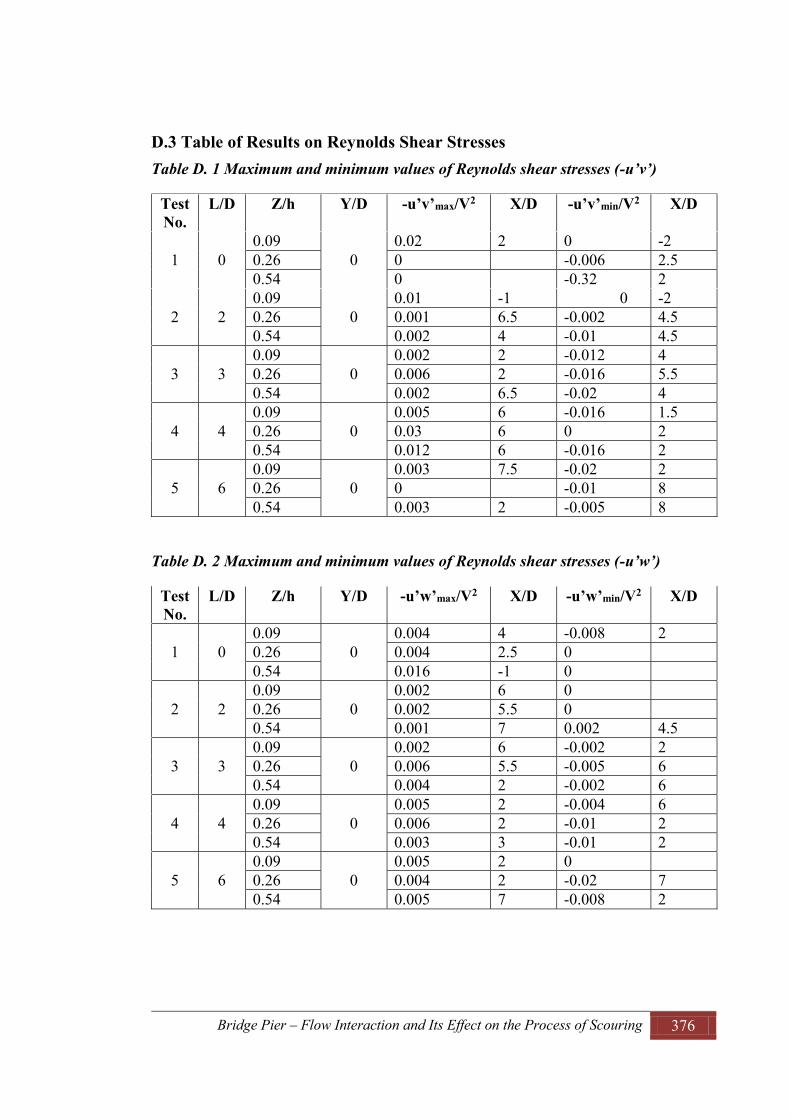
Bridge Pier – Flow Interaction and Its Effect on the Process of Scouring 376
D.3 Table of Results on Reynolds Shear Stresses Table D. 1 Maximum and minimum values of Reynolds shear stresses (-u’v’)
Test No.
L/D Z/h Y/D -u’v’max/V2 X/D -u’v’min/V2 X/D
1 0 0.09
0 0.02 2 0 -2
0.26 0 -0.006 2.5 0.54 0 -0.32 2
2 2 0.09
0 0.01 -1 0 -2
0.26 0.001 6.5 -0.002 4.5 0.54 0.002 4 -0.01 4.5
3 3 0.09
0 0.002 2 -0.012 4
0.26 0.006 2 -0.016 5.5 0.54 0.002 6.5 -0.02 4
4 4 0.09
0 0.005 6 -0.016 1.5
0.26 0.03 6 0 2 0.54 0.012 6 -0.016 2
5 6 0.09
0 0.003 7.5 -0.02 2
0.26 0 -0.01 8 0.54 0.003 2 -0.005 8
Table D. 2 Maximum and minimum values of Reynolds shear stresses (-u’w’)
Test No.
L/D Z/h Y/D -u’w’max/V2 X/D -u’w’min/V2 X/D
1 0 0.09
0 0.004 4 -0.008 2
0.26 0.004 2.5 0 0.54 0.016 -1 0
2 2 0.09
0 0.002 6 0
0.26 0.002 5.5 0 0.54 0.001 7 0.002 4.5
3 3 0.09
0 0.002 6 -0.002 2
0.26 0.006 5.5 -0.005 6 0.54 0.004 2 -0.002 6
4 4 0.09
0 0.005 2 -0.004 6
0.26 0.006 2 -0.01 2 0.54 0.003 3 -0.01 2
5 6 0.09
0 0.005 2 0
0.26 0.004 2 -0.02 7 0.54 0.005 7 -0.008 2

Bridge Pier – Flow Interaction and Its Effect on the Process of Scouring 377
Table D. 3 Maximum and minimum values of Reynolds shear stresses (-v’w’)
Test No.
L/D Z/h Y/D -v’w’max/V2 X/D -v’w’min/V2 X/D
1 0 0.09
0 0.004 2 0
0.26 0.014 2 0 0.54 0.02 3 0
2 2 0.09
0 0 -0.002 -1
0.26 0.003 4.5 0 0.54 0.003 5.5 0
3 3 0.09
0 0.003 6 -0.003 2
0.26 0.005 5.5 0 0.54 0.006 7 -0.003 4
4 4 0.09
0 0.008 1.5 0.005 6
0.26 0 -0.002 2 0.54 0.01 6 0
5 6 0.09
0 0.01 2 0
0.26 0.008 2 0 0.54 0.005 8 -0.005 3
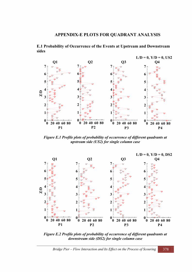
Bridge Pier – Flow Interaction and Its Effect on the Process of Scouring 378
APPENDIX-E PLOTS FOR QUADRANT ANALYSIS
E.1 Probability of Occurrence of the Events at Upstream and Downstream sides
L/D = 0, Y/D = 0, US2 Q1 Q2 Q3 Q4
Figure E.1 Profile plots of probability of occurrence of different quadrants at upstream side (US2) for single column case
L/D = 0, Y/D = 0, DS2 Q1 Q2 Q3 Q4
Figure E.2 Profile plots of probability of occurrence of different quadrants at downstream side (DS2) for single column case
0 20 40 60 80 10
1
2
3
4
5
6
7
P1
Z/D
0 20 40 60 800
1
2
3
4
5
6
7
P20 20 40 60 80
0
1
2
3
4
5
6
7
P30 20 40 60 80 1
0
1
2
3
4
5
6
7
P4
0 20 40 60 800
1
2
3
4
5
6
7
P1
Z/D
0 20 40 60 800
1
2
3
4
5
6
7
P20 20 40 60 80
0
1
2
3
4
5
6
7
P30 20 40 60 80 1
0
1
2
3
4
5
6
7
P4

Bridge Pier – Flow Interaction and Its Effect on the Process of Scouring 379
L/D = 1, Y/D = 0, US1 Q1 Q2 Q3 Q4
Figure E.3 Profile plots of probability of occurrence of different quadrants at upstream side (US1) of Column 1 for two columns case with L/D = 1
L/D = 1, Y/D = 0, US2
Q1 Q2 Q3 Q4
Figure E.4 Profile plots of probability of occurrence of different quadrants at upstream side (US2) of Column 1 for two columns case with L/D = 1
0 20 40 60 800
1
2
3
4
5
6
7
P1
Z/D
0 20 40 60 80 10
1
2
3
4
5
6
7
P20 20 40 60 80
0
1
2
3
4
5
6
7
P30 20 40 60 80
0
1
2
3
4
5
6
7
P4
0 20 40 60 800
1
2
3
4
5
6
7
P1
Z/D
0 20 40 60 800
1
2
3
4
5
6
7
P20 20 40 60 80
0
1
2
3
4
5
6
7
P30 20 40 60 80 1
0
1
2
3
4
5
6
7
P4

Bridge Pier – Flow Interaction and Its Effect on the Process of Scouring 380
L/D = 1, Y/D = 0, DS1 Q1 Q2 Q3 Q4
Figure E.5 Profile plots of probability of occurrence of different quadrants at downstream side (DS1) of Column 2 for two columns case with L/D = 1
L/D = 1, Y/D = 0, DS2 Q1 Q2 Q3 Q4
Figure E.6 Profile plots of probability of occurrence of different quadrants at downstream side (DS2) of Column 2 for two columns case with L/D = 1
0 20 40 60 800
1
2
3
4
5
6
7
P1
Z/D
0 20 40 60 800
1
2
3
4
5
6
7
P20 20 40 60 80
0
1
2
3
4
5
6
7
P30 20 40 60 80
0
1
2
3
4
5
6
7
P4
0 20 40 60 80 10
1
2
3
4
5
6
7
P1
Z/D
0 20 40 60 800
1
2
3
4
5
6
7
P20 20 40 60 80
0
1
2
3
4
5
6
7
P30 20 40 60 80
0
1
2
3
4
5
6
7
P4

Bridge Pier – Flow Interaction and Its Effect on the Process of Scouring 381
L/D = 2, Y/D = 0, US1 Q1 Q2 Q3 Q4
Figure E.7 Profile plots of probability of occurrence of different quadrants at upstream side (US1) of Column 1 for two columns case with L/D = 2
L/D = 2, Y/D = 0, US2 Q1 Q2 Q3 Q4
Figure E.8 Profile plots of probability of occurrence of different quadrants at upstream side (US2) of Column 1 for two columns case with L/D = 2
0 20 40 60 800
1
2
3
4
5
6
7
P1
Z/D
0 20 40 60 800
1
2
3
4
5
6
7
P20 20 40 60 80
0
1
2
3
4
5
6
7
P30 20 40 60 80
0
1
2
3
4
5
6
7
P4
0 20 40 60 800
1
2
3
4
5
6
7
P1
Z/D
0 20 40 60 800
1
2
3
4
5
6
7
P20 20 40 60 80
0
1
2
3
4
5
6
7
P30 20 40 60 80
0
1
2
3
4
5
6
7
P4
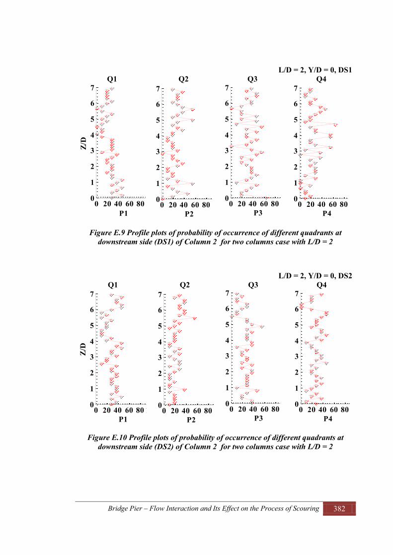
Bridge Pier – Flow Interaction and Its Effect on the Process of Scouring 382
L/D = 2, Y/D = 0, DS1 Q1 Q2 Q3 Q4
Figure E.9 Profile plots of probability of occurrence of different quadrants at downstream side (DS1) of Column 2 for two columns case with L/D = 2
L/D = 2, Y/D = 0, DS2 Q1 Q2 Q3 Q4
Figure E.10 Profile plots of probability of occurrence of different quadrants at downstream side (DS2) of Column 2 for two columns case with L/D = 2
0 20 40 60 800
1
2
3
4
5
6
7
P1
Z/D
0 20 40 60 80 10
1
2
3
4
5
6
7
P20 20 40 60 80
0
1
2
3
4
5
6
7
P30 20 40 60 80
0
1
2
3
4
5
6
7
P4
0 20 40 60 80 10
1
2
3
4
5
6
7
P1
Z/D
0 20 40 60 800
1
2
3
4
5
6
7
P20 20 40 60 80
0
1
2
3
4
5
6
7
P30 20 40 60 80
0
1
2
3
4
5
6
7
P4

Bridge Pier – Flow Interaction and Its Effect on the Process of Scouring 383
L/D = 2, Y/D = 0, B1 Q1 Q2 Q3 Q4
Figure E.11 Profile plots of probability of occurrence of different quadrants between two columns (B1) with L/D = 2
L/D = 3, Y/D = 0, US2 Q1 Q2 Q3 Q4
Figure E.12 Profile plots of probability of occurrence of different quadrants at upstream side (US2) of Column 1 for two columns case with L/D = 3
0 20 40 60 800
1
2
3
4
5
6
7
P1
Z/D
0 20 40 60 800
1
2
3
4
5
6
7
P20 20 40 60 80
0
1
2
3
4
5
6
7
P30 20 40 60 80 1
0
1
2
3
4
5
6
7
P4
0 20 40 60 800
1
2
3
4
5
6
7
P1
Z/D
0 20 40 60 800
1
2
3
4
5
6
7
P20 20 40 60 80
0
1
2
3
4
5
6
7
P30 20 40 60 80 1
0
1
2
3
4
5
6
7
P4
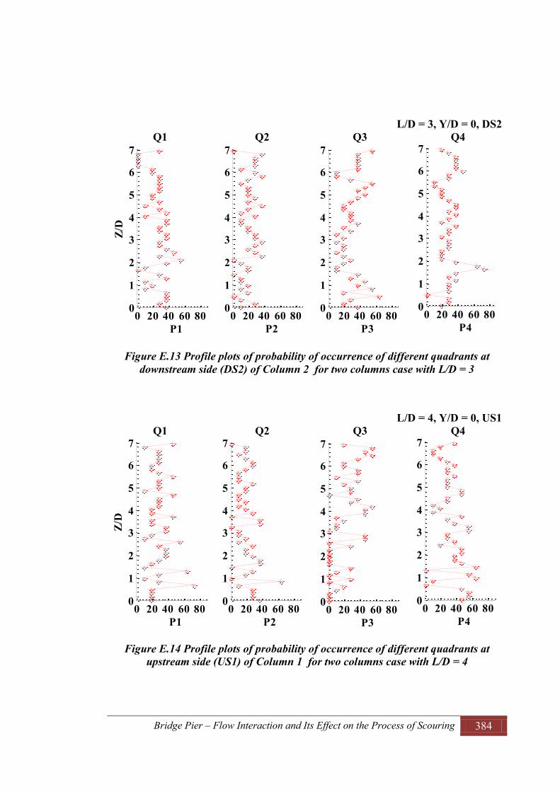
Bridge Pier – Flow Interaction and Its Effect on the Process of Scouring 384
L/D = 3, Y/D = 0, DS2 Q1 Q2 Q3 Q4
Figure E.13 Profile plots of probability of occurrence of different quadrants at downstream side (DS2) of Column 2 for two columns case with L/D = 3
L/D = 4, Y/D = 0, US1 Q1 Q2 Q3 Q4
Figure E.14 Profile plots of probability of occurrence of different quadrants at upstream side (US1) of Column 1 for two columns case with L/D = 4
0 20 40 60 800
1
2
3
4
5
6
7
P1
Z/D
0 20 40 60 800
1
2
3
4
5
6
7
P20 20 40 60 80
0
1
2
3
4
5
6
7
P30 20 40 60 80
0
1
2
3
4
5
6
7
P4
0 20 40 60 80 10
1
2
3
4
5
6
7
P1
Z/D
0 20 40 60 800
1
2
3
4
5
6
7
P20 20 40 60 80
0
1
2
3
4
5
6
7
P30 20 40 60 80
0
1
2
3
4
5
6
7
P4

Bridge Pier – Flow Interaction and Its Effect on the Process of Scouring 385
L/D = 4, Y/D = 0, DS1 Q1 Q2 Q3 Q4
Figure E.15 Profile plots of probability of occurrence of different quadrants at upstream side (US2) of Column 1 for two columns case with L/D = 4
L/D = 4, Y/D = 0, B1 Q1 Q2 Q3 Q4
Figure E.16 Profile plots of probability of occurrence of different quadrants between two columns (B1) with L/D = 4
0 20 40 60 800
1
2
3
4
5
6
7
P1
Z/D
0 20 40 60 800
1
2
3
4
5
6
7
P20 20 40 60 80
0
1
2
3
4
5
6
7
P30 20 40 60 80
0
1
2
3
4
5
6
7
P4
0 20 40 60 80 10
1
2
3
4
5
6
7
P1
Z/D
0 20 40 60 800
1
2
3
4
5
6
7
P20 20 40 60 80
0
1
2
3
4
5
6
7
P30 20 40 60 80
0
1
2
3
4
5
6
7
P4

Bridge Pier – Flow Interaction and Its Effect on the Process of Scouring 386
L/D = 4, Y/D = 0, B2 Q1 Q2 Q3 Q4
Figure E.17 Profile plots of probability of occurrence of different quadrants between two columns (B2) with L/D = 4
L/D = 6, Y/D = 0, US2 Q1 Q2 Q3 Q4
Figure E.18 Profile plots of probability of occurrence of different quadrants at upstream side (US2) of Column 1 for two columns case with L/D = 6
0 20 40 60 800
1
2
3
4
5
6
7
P1
Z/D
0 20 40 60 80 10
1
2
3
4
5
6
7
P20 20 40 60 80
0
1
2
3
4
5
6
7
P30 20 40 60 80
0
1
2
3
4
5
6
7
P4
0 20 40 60 800
1
2
3
4
5
6
7
P1
Z/D
0 20 40 60 800
1
2
3
4
5
6
7
P20 20 40 60 80
0
1
2
3
4
5
6
7
P30 20 40 60 80 1
0
1
2
3
4
5
6
7
P4

Bridge Pier – Flow Interaction and Its Effect on the Process of Scouring 387
L/D = 6, Y/D = 0, DS1 Q1 Q2 Q3 Q4
Figure E.19 Profile plots of probability of occurrence of different quadrants at downstream side (DS1) of Column 2 for two columns case with L/D = 6
L/D = 6, Y/D = 0, B1 Q1 Q2 Q3 Q4
Figure E.20 Profile plots of probability of occurrence of different quadrants between two columns (B1) with L/D = 6
0 20 40 60 800
1
2
3
4
5
6
7
P1
Z/D
0 20 40 60 800
1
2
3
4
5
6
7
P20 20 40 60 80
0
1
2
3
4
5
6
7
P30 20 40 60 80
0
1
2
3
4
5
6
7
P4
0 20 40 60 800
1
2
3
4
5
6
7
P1
Z/D
0 20 40 60 800
1
2
3
4
5
6
7
P20 20 40 60 80
0
1
2
3
4
5
6
7
P30 20 40 60 80
0
1
2
3
4
5
6
7
P4

Bridge Pier – Flow Interaction and Its Effect on the Process of Scouring 388
L/D = 6, Y/D = 0, B4 Q1 Q2 Q3 Q4
Figure E.21 Profile plots of probability of occurrence of different quadrants between two columns (B4) with L/D = 6
E.2 Profile Plots for Stress Fraction Contribution of the Events for the Production of Reynolds Stress.
L/D = 1, Y/D = 0, US1 Q1 Q2 Q3 Q4
0 20 40 60 800
1
2
3
4
5
6
7
P1
Z/D
0 20 40 60 800
1
2
3
4
5
6
7
P20 20 40 60 80
0
1
2
3
4
5
6
7
P30 20 40 60 80
0
1
2
3
4
5
6
7
P4
-1 -0.5 00
1
2
3
4
5
6
7
S1
Z/D
0 0.5 10
1
2
3
4
5
6
7
S2-1 -0.5 00
1
2
3
4
5
6
7
S30 0.5 1
0
1
2
3
4
5
6
7
S4

Bridge Pier – Flow Interaction and Its Effect on the Process of Scouring 389
Figure E.22 Profile plots for contribution of stress fraction of different quadrants for the production of Reynolds stress at upstream side (US1) of Column 1 for two
columns case with L/D = 1
L/D = 1, Y/D = 0, DS1 Q1 Q2 Q3 Q4
Figure E.23 Profile plots for contribution of stress fraction of different quadrants for the production of Reynolds stress at upstream side (DS1) of Column 2 for two
columns case with L/D = 1
L/D = 2, Y/D = 0, US1 Q1 Q2 Q3 Q4
Figure E.24 Profile plots for contribution of stress fraction of different quadrants for the production of Reynolds stress at upstream side (US1) of Column 1 for two
-1 -0.5 00
1
2
3
4
5
6
7
S1
Z/D
0 0.5 10
1
2
3
4
5
6
7
S2-1 -0.5 00
1
2
3
4
5
6
7
S30 0.5 1
0
1
2
3
4
5
6
7
S4
-1 -0.5 00
1
2
3
4
5
6
7
S1
Z/D
0 0.5 10
1
2
3
4
5
6
7
S2-1 -0.5 00
1
2
3
4
5
6
7
S30 0.5 1
0
1
2
3
4
5
6
7
S4

Bridge Pier – Flow Interaction and Its Effect on the Process of Scouring 390
columns case with L/D = 2
L/D = 2, Y/D = 0, DS1 Q1 Q2 Q3 Q4
Figure E.25 Profile plots for contribution of stress fraction of different quadrants for the production of Reynolds stress at upstream side (DS1) of Column 2 for two
columns case with L/D = 2
L/D = 2, Y/D = 0, B1 Q1 Q2 Q3 Q4
-1 -0.5 00
1
2
3
4
5
6
7
S1
Z/D
0 0.5 10
1
2
3
4
5
6
7
S2-1 -0.5 00
1
2
3
4
5
6
7
S30 0.5 1
0
1
2
3
4
5
6
7
S4
-1 -0.5 00
1
2
3
4
5
6
7
S1
Z/D
0 0.5 10
1
2
3
4
5
6
7
S2-1 -0.5 00
1
2
3
4
5
6
7
S30 0.5 1
0
1
2
3
4
5
6
7
S4

Bridge Pier – Flow Interaction and Its Effect on the Process of Scouring 391
Figure E.26 Profile plots for contribution of stress fraction of different quadrants for the production of Reynolds stress between two columns (B1) with L/D = 2
L/D = 4, Y/D = 0, US1 Q1 Q2 Q3 Q4
Figure E.27 Profile plots for contribution of stress fraction of different quadrants for the production of Reynolds stress at upstream side (US1) of Column 1 for two
columns case with L/D = 4
L/D = 4, Y/D = 0, DS1 Q1 Q2 Q3 Q4
-1 -0.5 00
1
2
3
4
5
6
7
S1
Z/D
0 0.5 10
1
2
3
4
5
6
7
S2-1 -0.5 00
1
2
3
4
5
6
7
S30 0.5 1
0
1
2
3
4
5
6
7
S4
-1 -0.5 00
1
2
3
4
5
6
7
S1
Z/D
0 0.5 10
1
2
3
4
5
6
7
S2-1 -0.5 00
1
2
3
4
5
6
7
S30 0.5 1
0
1
2
3
4
5
6
7
S4

Bridge Pier – Flow Interaction and Its Effect on the Process of Scouring 392
Figure E.28 Profile plots for contribution of stress fraction of different quadrants for the production of Reynolds stress at upstream side (DS1) of Column 2 for two
columns case with L/D = 4
L/D = 4, Y/D = 0, B1 Q1 Q2 Q3 Q4
Figure E.29 Profile plots for contribution of stress fraction of different quadrants for the production of Reynolds stress between two columns (B1) with L/D = 4
L/D = 4, Y/D = 0, B2 Q1 Q2 Q3 Q4
-1 -0.5 00
1
2
3
4
5
6
7
S1
Z/D
0 0.5 10
1
2
3
4
5
6
7
S2-1 -0.5 00
1
2
3
4
5
6
7
S30 0.5 1
0
1
2
3
4
5
6
7
S4
-1 -0.5 00
1
2
3
4
5
6
7
S1
Z/D
0 0.5 10
1
2
3
4
5
6
7
S2-1 -0.5 00
1
2
3
4
5
6
7
S30 0.5 1
0
1
2
3
4
5
6
7
S4

Bridge Pier – Flow Interaction and Its Effect on the Process of Scouring 393
Figure E.30 Profile plots for contribution of stress fraction of different quadrants for the production of Reynolds stress between two columns (B2) with L/D = 4
L/D = 6, Y/D = 0, US2 Q1 Q2 Q3 Q4
Figure E.31 Profile plots for contribution of stress fraction of different quadrants for the production of Reynolds stress at upstream side (US2) of Column 1 for two
columns case with L/D = 6
L/D = 6, Y/D = 0, DS1 Q1 Q2 Q3 Q4
Figure E.32 Profile plots for contribution of stress fraction of different quadrants for the production of Reynolds stress at upstream side (DS1) of Column 2 for two
columns case with L/D = 6
-1 -0.5 00
1
2
3
4
5
6
7
S1
Z/D
0 0.5 10
1
2
3
4
5
6
7
S2-1 -0.5 00
1
2
3
4
5
6
7
S30 0.5 1
0
1
2
3
4
5
6
7
S4
-1 -0.5 00
1
2
3
4
5
6
7
S1
Z/D
0 0.5 10
1
2
3
4
5
6
7
S2-1 -0.5 00
1
2
3
4
5
6
7
S30 0.5 1
0
1
2
3
4
5
6
7
S4

Bridge Pier – Flow Interaction and Its Effect on the Process of Scouring 394
L/D = 6, Y/D = 0, B1 Q1 Q2 Q3 Q4
Figure E.33 Profile plots for contribution of stress fraction of different quadrants for the production of Reynolds stress between two columns (B1) with L/D = 6
L/D = 6, Y/D = 0, B4 Q1 Q2 Q3 Q4
Figure E.34 Profile plots for contribution of stress fraction of different quadrants for the production of Reynolds stress between two columns (B4) with L/D = 6
-1 -0.5 00
1
2
3
4
5
6
7
S1
Z/D
0 0.5 10
1
2
3
4
5
6
7
S2-1 -0.5 00
1
2
3
4
5
6
7
S30 0.5 1
0
1
2
3
4
5
6
7
S4
-1 -0.5 00
1
2
3
4
5
6
7
S1
Z/D
0 0.5 10
1
2
3
4
5
6
7
S2-1 -0.5 00
1
2
3
4
5
6
7
S30 0.5 1
0
1
2
3
4
5
6
7
S4


