
Calendar Spread Options for Storable Commodities
Juheon Seok
PhD Candidate
Department of Agricultural Economics
Oklahoma State University
Stillwater, OK 74078
Phone: 405-744-9809
B. Wade Brorsen
Regents Professor and A.J. and Susan Jacques Chair
Department of Agricultural Economics
Oklahoma State University
Stillwater, OK 74078
Phone: 405-744-6836
Fax: 405-744-8210
Weiping Li
Watson Faculty Fellow of Finance & Professor
Department of Mathematics
Oklahoma State University
Stillwater, OK 74078
Selected Paper prepared for presentation at the Agricultural & Applied
Economics Association’s 2013 AAEA & CAES Joint Annual Meeting, Washington,
DC, August 4-6, 2013.
Copyright 2013 by Juheon Seok, B. Wade Brorsen, and Weiping Li. All rights reserved. Readers
may make verbatim copies of this document for non-commercial purposes by any means,
provided this copyright notice appears on all such copies.
1
Abstract
Many previous studies provide pricing models of options on futures spreads. However, none
of them fully reflect the economic reality that spreads can stay near full carry for long periods
of time. We suggest a new option pricing model that assumes that convenience yield follows
arithmetic Brownian motion and is truncated at zero. An analytical solution of the new
pricing model is obtained. We empirically test the new model by testing the truth of its
assumptions. We determine the distribution of calendar spreads and convenience yield for
Chicago Board of Trade corn calendar spread options. Panel unit root tests fail to reject the
null hypothesis of a unit root and thus support our assumption of arithmetic Brownian motion
as opposed to a mean-reverting process as is assumed in much past research. The assumption
that convenience yield is a normal distribution truncated at zero is only approximate as the
volatility of convenience yield never goes to zero and spreads tend to approach full carry, but
rarely reach full carry.
Key words: calendar spreads, corn, futures, panel unit root tests, options

2
Calendar Spread Options for Storable Commodities
1. Introduction
The Chicago Board of Trade (CBOT) offers trading of calendar spread options on futures in
wheat, corn, soybean, soybean oil, and soybean meal and the New York Mercantile Exchange
offers trading of calendar spread options on cotton and crude oil. Calendar spread options are a
new risk management tool. For example, storage facilities can purchase a calendar spread call
option to hedge the risk of futures spread narrowing or inverting. Grain elevators can use
calendar spread options to partially offset the risk of offering hedge-to-arrive contracts.
Options on calendar spreads cannot be replicated by combining two futures options with
different maturity dates. The reason is that calendar spread options are affected only by volatility
and value of the price relationship while any strategy to replicate the spread using futures options
is also sensitive to the value of the underlying commodity (CME Group). Despite such benefits,
so far the volume of calendar spread options traded has been low. Table 1 presents the volume of
CBOT futures, options, and calendar spread options on Aug 24, 2012. The daily volume across
all agricultural calendar spread option markets was 324 contracts, compared to the volume in the
corresponding futures contracts of 598,204. The small volume may at least be partly due to a
lack of understanding of how to value such options.
Earlier papers model the relationship between spot and futures prices and assume a mean
reverting convenience yield (Shimko; 1994, Schwartz; 1997). However, such an assumption is
doubtful for storable agricultural commodities since convenience yield may not follow a mean
reversion process. Gold does not have strong mean reversion (Schwartz 1997). Gold is typically

3
stored continually with no convenience yield so its spreads tend to remain at full carry1. Spreads
for agricultural markets will be close to full carry for long periods. Thus, there is a need to create
a more suitable option formula on calendar spreads for storable commodities that takes account
of all three factors: opportunity cost of interest, storage cost, and convenience yield.
In this article, we provide a calendar spread option pricing formula for storable commodities
that accounts for the lower bound on calendar spreads due to imposing no arbitrage opportunities
and also the assumptions and predictions of the model will be tested by determining the
distribution of convenience yield and calendar spreads using historical data.
To do this, we suggest a two factor model where nearby futures prices follow a geometric
Brownian motion and convenience yield is an arithmetic Brownian motion truncated at zero. The
valuation problem is solved like an option bear spread by combining a long call option and a
short call option with a strike price of zero. It is possible to test for distributional properties of
futures spread and convenience yield since spread is observable and convenience yield can be
estimated.
For the empirical test of model assumptions, daily CBOT corn futures prices are used
from 1975 to 2012. We only consider post-harvest spreads because full carry is never hit until
harvest. Using nonparametric regression, historical plots for corn show a downward trend after
harvest. Three-month Treasury Bills and the Prime rate are considered for interest rate and
storage costs are estimated using historical data on commercial storage rates between 1975 and
2012.
We estimated the convenience yield based on the theory of storage; convenience yield is
equal to spread plus interest forgone and physical storage cost. We determine the distribution of
1 The price difference between (futures) contracts with different maturity is prevented from exceeding the full cost
of carrying the commodity. Carrying costs include interest, insurance and storage.
4
spread and convenience yield. As expected, the indicate that calendar spreads are not normally or
log-normally distributed. The finding partially supports our assumption of truncated convenience
yield at zero. The price difference between two futures is often limited at 80~90% of full carry.
That is, full carry is rarely exceeded. Not quite reaching full carry can be explained by market
participants having varying interest cost or physical storage costs or possibly lack of an incentive
to take risks without some return.
Gibson and Schwartz (1990) develop a two-factor model taking account of stochastic
convenience yield in order to price oil contingent claims. They assume a mean reverting
convenience yield to explain an inverse relation between the level of inventory and the marginal
convenience yield. Schwartz (1997) extends this model to a three-factor model including a
stochastic interest rate and analyzes futures prices of copper, oil, and gold. He finds that copper
and oil have strong mean reversion while gold has weak mean reversion. Note that almost all
gold is stored, while long-term storage of copper and oil is less frequent.
Shimko (1994) derives a closed form solution to a futures spread option model, based on the
framework of Gibson and Schwartz (1990). Nakajima and Maeda (2007) generalize Shimko’s
model by introducing stochastic interest rates via Heath-Jarrow-Morton interest rate model
(Heath, Jarrow, and Morton 1992) as well as using the concept of future convenience yield.
Hinz and Fehr (2010) propose a commodity option pricing model considering no arbitrage in
both futures and physical commodity trading. They derive an upper bound observed in the
situation of contango limit by using an analogy between commodity and money markets. Their
work represents an important theoretical contribution, however, their empirical work is based on
using a shifted lognormal distribution and the Black-Scholes pricing formula. Their model does
5
satisfy the no arbitrage condition created by the contango limit, but it does not reflect the
economic reality that spreads will often stay near contango limit for long periods of time.
2. Theory
The theory of storage predicts the spread between futures and spot prices will be a function
of the interest forgone, S(t)R(t, T), the marginal storage cost, W(t, T), and the marginal
convenience yield, C(t, T):
(1) ( ) ( ) ( ) ( ) ( ) ( )
where F(t, T) is the futures price at time t for delivery at time T and S(t) denotes the spot price at
t. Some studies argue that the commodity spot price is not readily observable and use the futures
contract closest to maturity as a proxy for the spot price in empirical analysis for this reason
(Brennan 1958; Gibson and Schwartz 1990; Schwartz 1997; Hinz and Fehr 2010). This is a
strange argument since daily commodity spot prices are readily available. There are good reasons
for using the nearby as a proxy for spot prices, but it is not because spot prices do not exist.
Futures prices reflect the cheapest-to-deliver commodity and thus the spot price represented by
futures contracts can change over time. Also, as Irwin et al. (2011) discuss, grain futures markets
require the delivery of warehouse receipts or shipping certificates rather than the physical
delivery of grain. During much of 2008-2011, the price of deliverable warehouse receipts (or
shipping certificates) exceeded the spot price of grain and thus futures and spot prices diverged.
Inverse carrying charges have been observed in not only futures and spot prices but also
prices of distant and nearby futures. In this point, we extend the relationship in the theory of
storage from the futures and spot prices to the two futures prices. Nearby futures F(t, ) with
maturity is treated as the spot S(T1) at time and the periods for the interest rate, storage cost,

6
and convenience yield are the difference between deferred time and near time . Equation (1)
is rewritten as:
(2) ( ) ( ) ( ) ( ) ( ) ( )
where F(t, ) denotes the distant futures price at time t for delivery at and F(t, ) is the
nearby futures price. R(t, ), W(t, ), and C(t, ) denote the interest rate, the
marginal storage cost, and the marginal convenience yield for the period at time t,
respectively.
The marginal convenience yield approaches zero as the difference between nearby and distant
futures goes near full carry. Below full carry, the marginal convenience yield is positive which
means the nearby futures price exceeds the distant futures price. Sometimes, spreads for
agricultural markets remain near full carry for long periods. To explain this phenomenon, we
assume that convenience yield is truncated at full carry. The truncated convenience yield can be
represented as follows:
(3) ( ) ( ) ( )
We assume a calendar spread option model that takes account of the convenience yield being
truncated at full carry and derive a formula for options on calendar spreads. The CBOT traded
calendar spreads are defined as the nearby futures minus distant futures so that the spreads are
negative under contango. Equation (2) is multiplied by negative one to match the CBOT
definition of calendar spreads:
(4) ( ) ( ) ( ) ( ) ( ) ( )
The calendar spread option is an option on the price difference between two futures prices on
the same commodity with different maturities. When a calendar spread call option is exercised at

7
expiration, the buyer receives a long position in the nearby futures and a short position in the
distant futures. Consider a European calendar spread call option at time t. The call option expires
at time . i.e. the option expires prior to the delivery time of the nearby futures contract.
The payoff of the calendar spread call option with exercise price K is defined for
(5) ( ( ) ( ) )
As seen, the payoff of the call option is affected by the price difference between nearby and
distant futures prices. The theory of storage shows spreads between two futures is equal to
interest forgone plus storage costs minus convenience yield. We simplify the theory of storage
by assuming that both interest rate and storage costs are constant. That is, we only consider
nearby futures price and convenience yield to derive the payoff of the call option.
The European call price with the strike price K at maturity T is
(6) ( ) ( ( ) )
The resulting model is a two factor model. The nearby futures price is assumed to follow
geometric Brownian motion with drift µ and volatility . The convenience yield follows an
arithmetic Brownian motion that is truncated at zero. The drift of convenience yield is given by
and its volatility is given by . Two standard Brownian motions have constant correlation .
The two stochastic factors can be expressed as:
(7) ( ) ( ) ( ) ( )
(8) ( ) ( )
(9) ( ) ( )
where ( ) and ( ) are standard Wiener process. The stochastic volatility model of Heston
(1993) is one of the most popular option pricing models. Our model does not consider stochastic

8
volatility but the approach to derive the call option follows steps similar to Heston’s work; the
partial differential equation of the call price is obtained from two stochastic processes, the
similar solution required to solve the problem is provided by assuming specific functions for the
two probabilities, and characteristic functions are used to obtain probability functions. The value
of any asset ( ) must satisfy the partial differential equation (PDE) under no arbitrage
condition
(10)
A European call option satisfies the PDE (10) and a solution of pricing the call is
(11) ( ) ( )
where the probability and are the conditional probability that the option is in-the-money
Let and substitute the solution of (11) into the PDE (10). This leads to PDEs for and
(12)
(
)
( )
(
)
The probabilities and corresponding to the characteristic functions and are
(13)
∫
( )
We guess the characteristic functions
(14) ( ) ( ( ) ( ) )
where ( )
( )

9
( )
( )
√( ) ( )
for j=1,2 and
To handle convenience yield truncated at zero, we propose a second option for convenience yield
which follows arithmetic Brownian motion (Bachelier; 1990) and has a strike price of zero. We
specify the convenience yield ( ) satisfying at time t
(15) ( ) ( )
For , where ( ) denotes standard Brownian Motion, subscript B stands for
Bacheiler, and represents the volatility. The value of a European call option at maturity T
is
(16) ( ) ( ( ) )
where is the exercise price. Following the Bachelier framework, the convenience yield is
normally distributed with mean ( ) and variance . The call option at time is
(17) ( ) ( ( ) ) ( ( )
( ) √ ) ( ) √ (
( )
( ) √ )
where ( )
√
⁄ is the standard normal density function. Our purpose is a call option
with the strike price of zero. Substitute the strike price into zero.
(18) ( ) ( ) ( ( )
( ) √ ) ( ) √ (
( )
( ) √ )

10
( ) represents the second call option with the strike price of zero. By combining the long
call option from equation (11) and the short call option from equation (18), a long calendar
spread call option is
(19) ( ( ) ) ( )
where is the calendar spread call option and ( ( ) ) is the call option from the
combined stochastic processes of changes in interest costs due to the change in the nearby price
and convenience yield.
3. Data
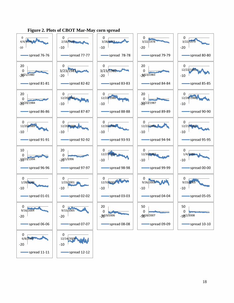
The data are daily corn futures prices between 1975 and 2012 from the Chicago Board of
Trade. Figures 1 through 5 depict the movement in Dec-Mar, Mar-May, July-Dec, and Dec-July
corn futures spreads, respectively. Dec-Mar, Mar-May, and Dec-July corn futures spreads are
mostly in contango in that corn futures spreads (nearby minus distant) are less than zero. The
July-Dec corn futures spread is across crop years and is mostly in backwardation where the
nearby is above the distant most of the time. Figure 1 is also used for visual estimated spread to
see if spread is at full carry. Nonparametric regression is used to verify the trend. In Figure 6,
Dec-Mar, May-July, and Dec-July spreads have a similar trend while Mar-May and July-Dec
spreads have a similar curve. One common trend is that all five futures spreads decrease as
maturity approaches. That is, historical corn spreads exhibit a downward trend during post-
harvest. This downward trend might reflect a risk premium. We only consider post-harvest
spreads for 100 days before expiration because full carry is never hit until harvest. Daily three-
month Treasury Bills and the Prime rate are used for interest rate from the Federal Reserve
System (FED) and annual storage costs are estimated using historical data on commercial storage

11
rates (Franken, Garcia, and Irwin 2009). The storage cost data are converted from yearly to daily
using the relevant SAS procedure. The sample period of storage costs and interest rate is 1975 -
2012. Table 2 summarizes the data for nearby and distant futures, calendar spread, interest rates,
and storage costs for each spread. The price of distant futures is above that of nearby futures
except July-Dec spread. Daily means of futures spread are between -20.01 and 5.2 where
negative sign is because spread is defined as nearby futures minus distant futures price. As
spread period is longer, the absolute mean of spread is larger. Absolute Dec-July spread is the
largest mean of -20.1. The mean of the Prime rate (8.3%) is higher than that of three-mouth
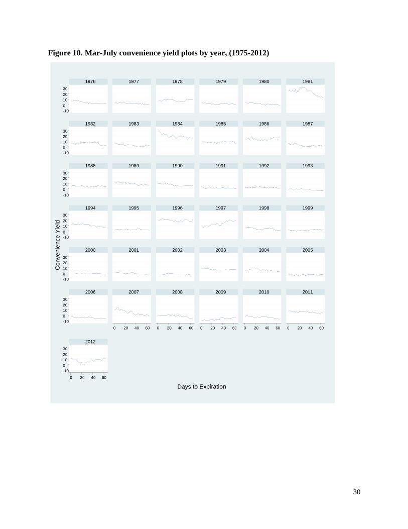
Treasury Bills (5.2%). The mean of convenience yield is between 1.2 and 25.7, which has a
positive value even though the minimum of convenience yield has negative value. Figure 8
through 12 present the implicit convenience yield plots for each year using the Prime rate.
Convenience yield is positive most of the time and negative convenience yield could occur from
underestimating physical storage costs during these years.
4. Methodology
We estimate descriptive statistics and test distributions for both the calendar spreads and
convenience yield. The distributional tests for spreads are conducted by tests of skewness (√ ),
kurtosis ( ), and an omnibus test (K2). Convenience yield is not directly observable.
Convenience yield is estimated following equation (4) as
(20) ( ) ( ( ) ( )) ( ) ( ) ( )
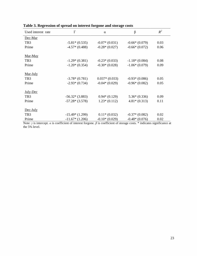
To test the above calculation we also regress spread against interest forgone and storage costs
(21) ( ) ( ) ( ) ( ) ( )
12
We analyze the distributional properties of convenience yield to investigate whether the
distribution of convenience yield is well approximated by a normal distribution that is truncated
at zero employing historical data. Descriptive statistics and test for distributions are conducted
for the estimated convenience yield.
We test for the presence of mean reversion in the spread and convenience yield for Dec-Mar,
Mar-May, Mar-July, July-Dec, and Dec-July. If spread or convenience yield is stable it implies
spread or convenience yield follows a mean reverting process as previous papers assume. The
data are cross sectional time series, where the years are the cross section and the days to maturity
is the time series. Stata provides several panel unit root tests such as Im-Pesaran- Shin (2003)
and Fisher-type (Choi 2001) tests for unbalanced panels. All of the tests are used to diagnose a
unit root. The null hypothesis is that the panels contain a unit root.
5. Empirical Results
We regress the spread against the interest forgone and storage costs with 3-month Treasury
Bills as well as the Prime rate (Table 3). Dec-Mar and Mar-July spread regressions show the
expected negative signs, but are mostly less than one in absolute value. The small coefficients
could be due to attenuation bias due to measurement error as well as not including convenience
yield in the regression. . The results show little consistent difference in the two interest rates.
Histograms for spread and convenience yield are presented in figure 7. For Dec-Mar, Mar-
May, Mar-July, and Dec-July spreads, the skewness is close to that of a normal distribution while
the relative kurtosis indicates a leptokurtic distribution. The histograms of convenience yield2
show a right tail and skewness to the right. Especially, July-Dec histograms of spread and
convenience yield more skew to right. Although the normality of convenience yield is rejected, it
2 The convenience yield is computed by the Prime rate times nearby futures prices plus storage costs.

13
is shown that the shape of the distribution provides modest support for assuming truncation at
zero once values less than zero are regarded as measurement noise. The empirical result shows
that calendar spreads are only close to full carry most of sample period and thus the price
differences between two futures are limited at 80~90% of full carry. It may be that convenience
yield has measurement noise due to estimating storage and interest costs. But, it also could be
that there is no economic incentive to run spreads all of the way to full carry. Table 4 reports
normality tests for spreads and convenience yield. All omnibus tests reject the null of a normal
distribution at the 5 % significance level in both five spreads and convenience yield.
Panel unit root test results are presented in table 6. Statistics for spreads and convenience
yield range between -2.18 and 1.29. We cannot reject the null hypotheses of spreads and
convenience yield having unit roots. This suggests that all the spreads and convenience yield do
not follow mean reversion.
6. Summary and Conclusion
The theory of storage says that calendar spreads on a storable commodity are the sum of the
opportunity cost of interest, the physical cost of storage, and convenience yield. We develop a
new calendar spread option pricing model in which convenience yield follows arithmetic
Brownian motion that is truncated at zero, nearby futures follow geometric Brownian motion,
and interest rates and the physical cost of storage are held constant. An analytical solution for the
two-factor model is obtained using steps similar to that used to derive the Heston stochastic
volatility model although our model does not assume stochastic volatility. The premium of a call
option on a calendar spread is then obtained as the sum of the premium of the two-factor model
minus the premium of call option on the convenience yield that has a strike price of zero.

14
We compute the implicit convenience yield to determine whether spreads are at full carry,
and regress spread against interest forgone and storage costs, and calculate convenience yield
according to the theory of storage. The Prime rate appears to provide a better estimate of full
carry than does U.S. Treasury Bill rates. Distributional tests are conducted for five calendar
spreads and convenience yield using the Prime rate as interest rate. The null hypothesis of
normality is rejected with both spread and convenience yield as expected. The histogram of
spread, however, is somewhat similar to a normal distribution. The distribution of convenience
yield is strongly skewed to the right which supports the assumption that full carry is acting as a
lower bound. The variance of estimated convenience yield does not go to zero and convenience
yield usually stops a little short of full carry. This result may reflect market participants that have
varying physical cost of storage and varying interest rates. Most commercial elevators are likely
net borrowers, but some producers may be net lenders. We conduct panel unit root tests for five
calendar spreads and convenience yield. The null hypothesis of a unit root cannot be rejected and
thus the results support our assumption of Brownian motion over the Gibson and Schwartz (1990)
assumption of mean reverting convenience yield. Thus, the model represents a considerable
improvement over past models. Future research will consider a four factor model where interest
rates and physical costs are also random. Future study will also extend the test for other
commodities and test the model using traded option premiums. The new calendar spread option
pricing model developed here has the potential to allow traders to lower bid-ask spreads, which
ultimately could increase volume in these markets much like has occurred with traders use of the
Black-Scholes model.

15
Table 1. The volume of Chicago Board of Trade calendar spread options and futures
Type Name Daily Volume a Monthly Volume
b
Futures Corn 217,347 6,825,321
Futures Soybean 140,842 5,195,821
Futures Soybean Meal 68,001 1,848,093
Futures Soybean Oil 91,190 2,394,547
Futures Wheat 80,824 2,404,137
SUM 598,204 18,667,919
Options Corn 151,021 3,537,600
Options Soybean 53,127 2,460,585
Options Soybean Meal 7,083 224,899
Options Soybean Oil 16,359 208,483
Options Wheat 18,858 620,709
SUM 246,448 7,052,276
CSO Consecutive Corn 235 6,981
CSO Consecutive Soybean 0 0
CSO Consecutive Soybean Meal 0 0
CSO Consecutive Soybean Oil 50 265
CSO Consecutive Wheat 0 3,225
CSO Corn July-Dec 0 458
CSO Corn Dec-July 0 511
CSO Corn Dec-Dec 8 0
CSO Soybean Jan-May 0 0
CSO Soybean July-Nov 0 0
CSO Soybean Aug-Nov 0 935
CSO Soybean Nov-July 0 81
CSO Soybean Nov-Nov 0 0
CSO Soy Meal July-Dec 0 0
CSO Soy Oil July-Dec 0 0
CSO Wheat July-July 0 0
CSO Wheat July-Dec 0 0
CSO Wheat Dec-July 0 725
SUM 324 13,181 a The daily data are from Aug 24, 2012.
b The monthly data are from July 2012.

16
Table 2. Summary statistics
Variable Sample Period Mean Standard
Deviation Minimum Maximum
Dec-Mar CBOT Corn
Dec Futures (¢/bu) 10/10/1975-11/18/2011 279.0 101.9 161.5 775.3
Mar Futures (¢/bu) 10/10/1975-11/18/2011 289.2 102.9 173.0 787.3
Dec-Mar Spread (¢/bu) 10/10/1975-11/18/2011 -10.1 3.7 -19.5 3.8
ln(Dec/Mar) Spread (¢/bu) 10/10/1975-11/18/2011 0.0 0.0 -0.1 0.0
Dec-Mar Implicit Convenience Yield 10/10/1975-11/18/2011 1.5 4.1 -8.3 19.4
Three-month TB (%) 10/10/1975-11/18/2011 5.2 3.3 0.0 15.9
Prime rate(%) 10/10/1975-11/18/2011 8.3 3.3 3.3 20.5
Storage Costs (¢/bu) 10/10/1975-11/18/2011 6.2 1.0 4.5 9.0
Mar-May CBOT Corn
Mar Futures (¢/bu) 11/12/1975-2/18/2012 287.5 101.8 142.8 712.8
May Futures (¢/bu) 11/12/1975-2/18/2012 294.2 102.5 150.8 723.0
Mar-May Spread (¢/bu) 11/12/1975-2/18/2012 -6.7 2.9 -13.8 2.5
ln(Mar/May) Spread (¢/bu) 11/12/1975-2/18/2012 0.0 0.0 -0.1 0.0
Mar-May Implicit Convenience Yield 11/12/1975-2/18/2012 1.2 3.1 -5.2 12.6
Three-month TB (%) 11/12/1975-2/18/2012 5.2 3.4 0.0 17.1
Prime rate(%) 11/12/1975-2/18/2012 8.3 3.5 3.3 21.5
Storage Costs (¢/bu) 11/12/1975-2/18/2012 4.1 0.7 3.0 6.0
Mar-July CBOT Corn
Mar Futures (¢/bu) 11/12/1975-2/16/2012 287.5 101.8 142.8 712.8
July Futures (¢/bu) 11/12/1975-2/16/2012 298.7 102.7 155.3 726.8
Mar-July Spread (¢/bu) 11/12/1975-2/16/2012 -11.2 5.9 -24.3 6.3
ln(Mar/July) Spread (¢/bu) 11/12/1975-2/16/2012 0.0 0.0 -0.1 0.0
Mar-July Implicit Convenience Yield 11/12/1975-2/16/2012 4.7 6.9 -10.0 31.6
Three-month TB (%) 11/12/1975-2/16/2012 5.2 3.4 0.0 17.1
Prime rate(%) 11/12/1975-2/16/2012 8.3 3.5 3.3 21.5
Storage Costs (¢/bu) 11/12/1975-2/16/2012 8.2 1.4 6.0 12.0
July-Dec CBOT Corn
July Futures (¢/bu) 3/12/1976-6/19/2012 307.1 119.6 160.8 787.0
Dec Futures (¢/bu) 3/12/1976-6/19/2012 301.9 105.2 171.8 780.0
July-Dec Spread (¢/bu) 3/12/1976-6/19/2012 5.2 30.5 -34.3 159.3
ln(July/Dec) Spread (¢/bu) 3/12/1976-6/19/2012 0.0 0.1 -0.1 0.4
July-Dec Implicit Convenience Yield 3/12/1976-6/19/2012 25.7 32.3 -9.1 186.6
Three-month TB (%) 3/12/1976-6/19/2012 5.2 3.5 0.0 17.0
Prime rate(%) 3/12/1976-6/19/2012 8.3 3.7 3.3 20.5
Storage Costs (¢/bu) 3/12/1976-6/19/2012 10.4 1.8 7.5 15.0
Dec-July CBOT Corn
Dec Futures (¢/bu) 8/12/1976-11/16/2011 279.0 101.7 161.5 775.3
July Futures (¢/bu) 8/12/1976-11/16/2011 299.1 103.2 182.0 794.0
Dec-July Spread (¢/bu) 8/12/1976-11/16/2011 -20.1 8.9 -42.0 11.0
ln(Dec/July) Spread (¢/bu) 8/12/1976-11/16/2011 -0.1 0.0 -0.1 0.0
Dec-July Implicit Convenience Yield 8/12/1976-11/16/2011 7.2 10.4 -18.8 47.8
Three-month TB (%) 8/12/1976-11/16/2011 5.2 3.3 0.0 15.9
Prime rate(%) 8/12/1976-11/16/2011 8.3 3.3 3.3 20.5
Storage Costs (¢/bu) 8/12/1976-11/16/2011 14.4 2.3 10.5 21.0
Note: Implicit convenience yield is computed by the Prime rate times nearby futures prices plus storage costs. All data are daily.

17
Figure 1. Plots of CBOT Dec-Mar corn spread
-20
010/10/1975
spread 76-77
-50
0 12/22/1980
spread 81-82
-20
0
9/20/1985
spread 86-87
-20
0
9/20/1990
spread 91-92
-10
0
9/21/1995
spread 96-97
-20
0
11/17/2000
spread 01-02
-20
0
5/31/2005
spread 06-07
-20
0
12/14/2009
spread 11-12
-10
01/6/1977
spread 77-78
-20
012/28/1981
spread 82-83
-20
0
9/22/1986
spread 87-88
-20
0
9/20/1991
spread 92-93
-20
0
9/25/1996
spread 97-98
-20
0
20
9/20/2001
spread 02-03
-20
0
3/27/2006
spread 07-08
-20
01/4/1978
spread 78-79
-20
0
20
12/23/1982
spread 83-84
-20
0
20
9/28/1987
spread 88-89
-10
0
9/22/1992
spread 93-94
-20
0
9/22/1997
spread 98-99
-10
0
3/15/2002
spread 03-04
-50
0
3/16/2007
spread 08-09
-20
012/20/78
spread 79-80
-20
0
10/21/1983
spread 84-85
-10
0
9/26/1988
spread 89-90
-20
09/22/1993
spread 94-95
-20
0
9/22/1998
spread 99-00
-20
0
6/26/2003
spread 04-05
-20
0
20
3/19/2007
spread 09-10
-20
012/19/1979
spread 80-81
-20
0
9/20/1984
spread 85-86
-20
0
9/21/1989
spread 90-91
-10
0
9/22/1994
spread 95-96
-20
0
10/29/1999
spread 00-01
-20
0
7/19/2004
spread 05-06
-20
0
4/2/2009
spread 10-11
18
Figure 2. Plots of CBOT Mar-May corn spread
-10
0
4/4/1975
spread 76-76
-20
0
20
3/21/1980
spread 81-81
-20
0
20
12/20/1984
spread 86-86
-10
012/20/1989
spread 91-91
-10
0
10
12/21/1994
spread 96-96
-10
01/28/2000
spread 01-01
-20
09/16/2004
spread 06-06
-20
06/8/2009
spread 11-11
-10
02/18/1976
spread 77-77
-20
0
3/23/1981
spread 82-82
-10
012/20/1985
spread 87-87
-10
012/20/1990
spread 92-92
-20
0
20
2/1/1996
spread 97-97
-10
01/23/2001
spread 02-02
-20
09/15/2005
spread 07-07
-10
012/14/2009
spread 12-12
-10
03/28/1977
spread 78-78
-20
0
3/23/1982
spread 83-83
-10
012/22/1986
spread 88-88
-10
012/26/1991
spread 93-93
-10
012/27/1996
spread 98-98
-10
012/31/2001
spread 03-03
-20
0
20
5/19/2006
spread 08-08
-20
03/22/1978
spread 79-79
-20
0
20
1/13/1983
spread 84-84
-20
0
20
12/22/1987
spread 89-89
-10
012/22/1992
spread 94-94
-10
012/30/1997
spread 99-99
-10
09/26/2002
spread 04-04
-50
0
50
9/18/2007
spread 09-09
-20
03/22/1979
spread 80-80
-10
012/22/1983
spread 85-85
-10
012/28/1988
spread 90-90
-10
012/21/1993
spread 95-95
-10
01/4/1999
spread 00-00
-10
09/23/2003
spread 05-05
-50
0
50
4/2/2008
spread 10-10

19
Figure 3. Plots of CBOT Mar-July corn spread
-20
0
20
7/17/1975
spread 76-76
-50
0
50
5/22/1980
spread 81-81
-20
0
20
3/21/1985
spread 86-86
-20
0
3/22/1990
spread 91-91
-20
0
20
9/22/1994
spread 96-96
-20
0
11/9/1999
spread 01-01
-50
0
7/19/2004
spread 06-06
-20
0
4/2/2009
spread 11-11
-20
0
7/14/1976
spread 77-77
-50
0
5/26/1981
spread 82-82
-20
0
3/20/1986
spread 87-87
-20
0
3/21/1991
spread 92-92
-20
0
20
10/5/1995
spread 97-97
-20
0
11/17/2000
spread 02-02
-50
0
5/31/2005
spread 07-07
-20
0
12/14/2009
spread 12-12
-10
0
7/18/1977
spread 78-78
-50
0
5/20/1982
spread 83-83
-20
0
3/23/1987
spread 88-88
-20
0
3/23/1992
spread 93-93
-20
0
9/25/1996
spread 98-98
-20
0
20
9/20/2001
spread 03-03
-50
0
50
3/27/2006
spread 08-08
-20
0
5/22/1978
spread 79-79
-50
0
50
3/24/1983
spread 84-84
-50
0
50
3/23/1988
spread 89-89
-10
0
1/21/1993
spread 94-94
-20
0
9/22/1997
spread 99-99
-20
0
20
3/15/2002
spread 04-04
-50
0
50
3/16/2007
spread 09-09
-50
0
5/22/1979
spread 80-80
-20
0
3/22/1984
spread 85-85
-20
0
3/22/1989
spread 90-90
-20
0
12/21/1993
spread 95-95
-20
0
9/22/1998
spread 00-00
-20
0
20
7/23/2003
spread 05-05
-50
0
50
3/19/2007
spread 10-10

20
Figure 4. Plots of CBOT July-Dec corn spread
0
50
10/7/1975
spread 76-76
-100
0
100
9/22/1980
spread 81-81
0
50
7/23/1985
spread 86-86
-50
0
50
5/24/1990
spread 91-91
0
100
10/5/1995
spread 97-97
-50
0
50
7/26/2000
spread 02-02
-100
0
100
2/24/2005
spread 07-07
0
200
6/8/2009
spread 12-12
-50
0
50
10/1/1976
spread 77-77
-20
0
20
9/24/1981
spread 82-82
-50
0
50
7/23/1986
spread 87-87
-50
0
50
5/22/1991
spread 92-92
-50
0
50
8/15/1996
spread 98-98
-50
0
50
6/7/2001
spread 03-03
-100
0
100
1/30/2006
spread 08-08
-20
0
20
10/3/1977
spread 78-78
-100
0
100
8/23/1982
spread 83-83
-50
0
50
7/23/1987
spread 88-88
-50
0
50
4/6/1992
spread 93-93
-50
0
50
5/6/1997
spread 99-99
-50
0
50
1/2/2002
spread 04-04
-200
0
200
7/25/2006
spread 09-09
-20
09/21/1978
spread 79-79
0
100
8/2/1983
spread 84-84
0
100
5/26/1988
spread 89-89
0
50
1/21/1993
spread 94-94
-50
0
50
8/10/1998
spread 00-00
-100
0
100
7/23/2003
spread 05-05
-100
0
100
2/7/2007
spread 10-10
-50
09/20/1979
spread 80-80
0
50
7/23/1984
spread 85-85
0
50
5/22/1989
spread 90-90
0
200
5/27/1994
spread 96-96
-50
0
50
11/9/1999
spread 01-01
-100
0
100
5/25/2004
spread 06-06
-200
0
200
7/10/2008
spread 11-11

21
Figure 5. Plots of CBOT Dec-July corn spread
-50
0
7/14/1976
spread 76-77
-50
0
5/26/1981
spread 81-82
-50
0
3/20/1986
spread 86-87
-50
0
3/21/1991
spread 91-92
-20
0
10/5/1995
spread 96-97
-50
0
6/14/2001
spread 02-03
-50
0
2/6/2006
spread 07-08
-20
0
7/18/1977
spread 77-78
-50
0
5/20/1982
spread 82-83
-50
0
3/23/1987
spread 87-88
-50
0
3/23/1992
spread 92-93
-50
0
8/15/1996
spread 97-98
-50
0
1/7/2002
spread 03-04
-100
0
100
8/1/2006
spread 08-09
-50
0
5/22/1978
spread 78-79
-50
0
50
3/24/1983
spread 83-84
-50
0
50
3/23/1988
spread 88-89
-20
0
1/21/1993
spread 93-94
-50
0
4/28/1997
spread 98-99
-50
0
7/30/2003
spread 04-05
-50
0
50
2/14/2007
spread 09-10
-50
0
5/22/1979
spread 79-80
-50
0
3/22/1984
spread 84-85
-20
0
3/22/1989
spread 89-90
-50
0
12/21/1993
spread 94-95
-50
0
8/10/1998
spread 99-00
-50
0
6/2/2004
spread 05-06
-50
0
7/17/2008
spread 10-11
-50
0
5/22/1980
spread 80-81
-50
0
3/21/1985
spread 85-86
-50
0
3/22/1990
spread 90-91
-50
0
50
5/27/1994
spread 95-96
-50
0
8/2/2000
spread 01-02
-50
0
3/3/2005
spread 06-07
-50
0
6/15/2009
spread 11-12

22
Figure 6. Nonparametric regression of corn spread versus days to expiration
Dec-Mar corn spread (cents/bu.)
Mar-May corn spread (cents/bu.)
May-July corn spread (cents/bu.)
July-Dec corn spread (cents/bu.)
Dec-July corn spread (cents/bu.)
23
Table 3. Regression of spread on interest forgone and storage costs
Used interest rate Γ α β R2
Dec-Mar
TB3 -5.81* (0.535) -0.07* (0.031) -0.66* (0.079) 0.03
Prime -4.57* (0.488) -0.28* (0.027) -0.66* (0.072) 0.06
Mar-May
TB3 -1.29* (0.381) -0.23* (0.033) -1.18* (0.084) 0.08
Prime -1.20* (0.354) -0.30* (0.028) -1.06* (0.079) 0.09
Mar-July
TB3 -3.78* (0.781) 0.037* (0.033) -0.93* (0.086) 0.05
Prime -2.93* (0.734) -0.04* (0.029) -0.96* (0.082) 0.05
July-Dec
TB3 -56.32* (3.883) 0.94* (0.129) 5.36* (0.336) 0.09
Prime -57.28* (3.578) 1.23* (0.112) 4.81* (0.313) 0.11
Dec-July
TB3 -15.49* (1.299) 0.11* (0.032) -0.37* (0.082) 0.02
Prime -11.67* (1.206) -0.10* (0.029) -0.48* (0.076) 0.02 Note: γ is intercept. α is coefficient of interest forgone. β is coefficient of storage costs. * indicates significance at
the 5% level.

24
Figure 7. Histograms of spread and convenience yield, (1975-2012)
Note: Convenience yield is computed as the spread minus the Prime rate times nearby futures price and also minus
storage costs.
Dec-Mar Mar-May

25
Figure 7. Histograms of spread and convenience yield, (1975-2012) continued
Note: Convenience yield is computed as the spread minus the Prime rate times nearby futures price and also minus
storage costs.
Mar-July July-Dec

26
Figure 7. Histograms of spread and convenience yield, (1975-2012) continued
Note: Convenience yield is computed as the spread minus the Prime rate times nearby futures price and also minus
storage costs.
Dec-July

27
Table 4. Distribution for corn futures spread and convenience yield
Obs. Skewness Kurtosis Kolmogorov-
Smirnov Cramer-von Mises Anderson-Darling
Dec-Mar Dec-Mar Spread (c/bu) 2552 -0.12 0.45 0.01* 0.005* 0.005*
ln(Dec/Mar) Spread (¢/bu) 2552 0.03 0.0002 0.01* 0.005* 0.005*
Dec-Mar Implicit Convenience Yield 2552 0.88 1.48 0.01* 0.005* 0.005*
Mar-May
Mar-May Spread (¢/bu) 2500 0.18 -0.06 0.01* 0.005* 0.005*
ln(Mar/May) Spread (¢/bu) 2500 0.26 -0.48 0.01* 0.005* 0.005*
Mar-May Implicit Convenience Yield 2500 0.96 0.92 0.01* 0.005* 0.005*
Mar-July
Mar-July Spread (¢/bu) 2500 0.31 -0.18 0.01* 0.005* 0.005*
ln(Mar/May) Spread (¢/bu) 2500 0.32 -0.61 0.01* 0.005* 0.005*
Mar-July Implicit Convenience Yield 2500 6.89 1.27 0.01* 0.005* 0.005*
July-Dec
July-Dec Spread (¢/bu) 2587 2.16 5.02 0.01* 0.005* 0.005*
ln(July/Dec) Spread (¢/bu) 2587 1.46 2.62 0.01* 0.005* 0.005*
July-Dec Implicit Convenience Yield 2587 2.09 4.71 0.01* 0.005* 0.005*
Dec-July
Dec-July Spread (¢/bu) 2479 -0.13 0.23 0.01* 0.005* 0.005*
ln(Dec/July) Spread (¢/bu) 2479 0.15 -0.49 0.01* 0.005* 0.005*
Dec-July Implicit Convenience Yield 2479 0.77 0.87 0.01* 0.005* 0.005*
Note: Implicit convenience yield is computed as the spread minus the Prime rate times nearby futures price and also minus storage costs. * indicates rejection of
the null hypothesis of normality at the 5% level.

28
Figure 8. Dec-Mar convenience yield plots by year, (1975-2012)
-10
0
10 2
0
-10
0
10 2
0
-10
0
10 2
0
-10
0
10 2
0
-10
0
10 2
0
-10
0
10 2
0
0 20 40 60 80 0 20 40 60 80 0 20 40 60 80 0 20 40 60 80 0 20 40 60 80 0 20 40 60 80
1976 1977 1978 1979 1980 1981
1982 1983 1984 1985 1986 1987
1988 1989 1990 1991 1992 1993
1994 1995 1996 1997 1998 1999
2000 2001 2002 2003 2004 2005
2006 2007 2008 2009 2010 2011
Co
nve
nie
nce
Yie
ld
Days to Expiration

29
Figure 9. Mar-May convenience yield plots by year, (1975-2012)
-5 0 5 10 15
-5 0 5 10 15
-5 0 5 10 15
-5 0 5 10 15
-5 0 5 10 15
-5 0 5 10 15
-5 0 5 10 15
0 20 40 60 0 20 40 60 0 20 40 60 0 20 40 60 0 20 40 60
0 20 40 60
1976 1977 1978 1979 1980 1981
1982 1983 1984 1985 1986 1987
1988 1989 1990 1991 1992 1993
1994 1995 1996 1997 1998 1999
2000 2001 2002 2003 2004 2005
2006 2007 2008 2009 2010 2011
2012
Con
ve
nie
nce
Yie
ld
Yie
ld
Days to Expiration
30
Figure 10. Mar-July convenience yield plots by year, (1975-2012)
-10 0 10 20 30
-10 0 10 20 30
-10 0 10 20 30
-10 0 10 20 30
-10 0 10 20 30
-10 0 10 20 30
-10 0 10 20 30
0 20 40 60 0 20 40 60 0 20 40 60 0 20 40 60 0 20 40 60
0 20 40 60
1976 1977 1978 1979 1980 1981
1982 1983 1984 1985 1986 1987
1988 1989 1990 1991 1992 1993
1994 1995 1996 1997 1998 1999
2000 2001 2002 2003 2004 2005
2006 2007 2008 2009 2010 2011
2012
Con
ve
nie
nce
Yie
ld
Yie
ld
Days to Expiration

31
Figure 11. July-Dec convenience yield plots by year, (1975-2012)
0 50 100 150 200
0 50 100 150 200
0 50 100 150 200
0 50 100 150 200
0 50 100 150 200
0 50 100 150 200
0 20 40 60 80 0 20 40 60 80 0 20 40 60 80 0 20 40 60 80 0 20 40 60 80
0 20 40 60 80 0 20 40 60 80
1976 1977 1978 1979 1980 1981 1982
1983 1984 1985 1986 1987 1988 1989
1990 1991 1992 1993 1994 1995 1996
1997 1998 1999 2000 2001 2002 2003
2004 2005 2006 2007 2008 2009 2010
2011 2012
Con
ve
nie
nce
Yie
ld
Days to Expiration

32
Figure 12. Dec-July Convenience Yield Plots by year, (1975-2012)
-20 0 20 40
-20 0 20 40
-20 0
20 40
-20 0 20 40
-20 0 20 40
-20 0 20 40
0 20 40 60 0 20 40 60 0 20 40 60 0 20 40 60 0 20 40 60 0 20 40 60
1976 1977 1978 1979 1980 1981
1982 1983 1984 1985 1986 1987
1988 1989 1990 1991 1992 1993
1994 1995 1996 1997 1998 1999
2000 2001 2002 2003 2004 2005
2006 2007 2008 2009 2010 2011
Con
ve
nie
nce
Yie
ld
Yie
ld
Days to Expiration

33
Table 6. Panel Unit Root Tests in Corn Dec-Mar Futures Spread and Convenience Yield,
(1975-2006)
Variable 3-Month Treasury Bill (TB) Prime
Dec-Mar Futures Spread
Im-Pesaran-Shin Test -1.39 (0.08) -1.40 (0.08)
Fisher-type unit-root test -0.40 (0.35) 0.39 (0.35)
Dec-Mar Implicit Convenience Yield
Im-Pesaran-Shin Test 0.91 (0.18) -1.17 (0.12)
Fisher-type unit-root test -0.28 (0.61) -0.35 (0.64)
Mar-May Futures Spread
Im-Pesaran-Shin Test - -
Fisher-type unit-root test 0.31 (0.38) -0.83 (0.79)
Mar-May Implicit Convenience Yield
Im-Pesaran-Shin Test - -
Fisher-type unit-root test 1.36 (0.09) 0.33 (0.37)
Mar-July Futures Spread
Im-Pesaran-Shin Test -1.50 (0.07) -
Fisher-type unit-root test -0.68 (0.75) -0.68 (0.75)
Mar-July Implicit Convenience Yield
Im-Pesaran-Shin Test -0.36 (0.36) -0.50 (0.31)
Fisher-type unit-root test -0.64 (0.74) -0.45 (0.67)
July-Dec Futures Spread
Im-Pesaran-Shin Test -0.12 (0.45) -0.12 (0.45)
Fisher-type unit-root test 1.28 (0.09) 1.28 (0.09)
July-Dec Implicit Convenience Yield
Im-Pesaran-Shin Test -0.06 (0.48) -0.31 (0.38)
Fisher-type unit-root test 0.85 (0.19) 1.29 (0.09)
Dec-July Futures Spread
Im-Pesaran-Shin Test 0.22 (0.59) -0.03 (0.49)
Fisher-type unit-root test -0.57 (0.72) -0.48 (0.68)
Dec-July Implicit Convenience Yield
Im-Pesaran-Shin Test 0.95 (0.83) 0.78 (0.78)
Fisher-type unit-root test -1.72 (0.96) -1.43 (0.92) Note: The null hypothesis is that panels contain a unit root and thus the null hypothesis is not rejected using any of
the tests. Numbers in parentheses indicate p-values.

34
References
Bachelier, L. 1900. “ThCorie de la spkculation.” Annales de 1’Ecole Superieure, 17:21-86.
Translated in Cootner, P. H., ed. 1964. The Random Character of Stock Market Prices.
Cambridge MA: MIT Press, pp.17-78.
Black, F., and Scholes, M. 1973. “The Pricing of Options and Corporate Liabilities.” Journal of
Political Economy 81: 637–654.
Brennan, M. J. 1958. “The Supply of Storage.” The American Economic Review 48: 50–72.
Chicago Mercantile Exchange (CME) Group. “Grain and Oilseed Calendar Spread Options.”
accessible at http://www.cmegroup.com/trading/agricultural/files/AC-
357_CSO_Sell_Sheet-FC_3.pdf
Commandeur, J.J., and Koopman, S.J. 2007. An Introduction to State Space Time Series
Analysis. New York: Oxford University Press.
Fama, E.F., and French, K.R. 1987. “Commodity Futures Prices: Some Evidence on Forecast
Power, Premiums, and the Theory of Storage.” The Journal of Business 60: 55–73.
Franken, J.R.V., P. Garcia, and S.H. Irwin. 2009. “Is Storage at a Loss Merely an Illusion of
Spatial Aggregation?” Journal of Agribusiness 27:65-84.
Gibson, R., and Schwartz, E. 1990. “Stochastic Convenience Yield and the Pricing of Oil
Contingent Claims.” Journal of Finance 45: 959–976.
de Goeij, W.J. 2008. “Modeling Forward Curves for Seasonal Commodities

35
with an Application to Calendar Spread Options.” PhD dissertation, Free University of
Amsterdam.
Heston, S.L. 1993. "A Closed-Form Solution for Options with Stochastic Volatility with
Applications to Bond and Currency Options." The Review of Financial Studies 6: 327–343.
Heath, D., Jarrow, R. A., and Morton, A.J. 1992. “Bond Pricing and the Term Structure of
Interest Rates: A New Methodology for Contingent Claims Valuation.” Econometrica 60:
77–105.
Hinz, J., and Fehr, M. 2010. “Storage Costs in Commodity Option Pricing.” SIAM Journal on
Financial Mathematics 1: 729-751.
Irwin, S.H., Garcia, P., Good, D.L., and Kunda, L.E. 2011. “Spreads and Non-convergence in
Chicago Board of Trade Corn, Soybean, and Wheat Futures: Are Index Funds to Blame?”
Applied Economic Perspectives and Policy 33: 116–142.
Nakajima K., and Maeda A. 2007. “Pricing Commodity Spread Options with Stochastic Term
Structure of Convenience Yields and Interest Rates.” Asia-Pacific Financial Markets 14:
157-184.
Murphy, J.A. 1990. “A Modification and Re-Examination of the Bachelier Option Pricing
Model.” American Economist 34: 34–41.
Poitras, G. 1990. “The Distribution of Gold Futures Spreads.” The Journal of Futures Markets
10: 643–659.
____. 1998. “Spread Options, Exchange Options, and Arithmetic Brownian Motion.” Journal of
Futures Markets 18: 487-517.

36
Schachermayer, W., and Teichmann J. 2008. “How Close Are the Option Pricing Formulas of
Bachelier and Black-Merton-Scholes?” Mathematical Finance 18:155-170.
Schwartz, E.S. 1997. "The Stochastic Behavior of Commodity Prices: Implications for Valuation
and Hedging." Journal of Finance 52: 923-973.
Shimko, D. 1994. “Options on Futures Spreads: Hedging, Speculation and Valuation.” The
Journal of Futures Markets 14: 183–213.
Working, H. 1949. “The Theory of Price of Storage.” American Economic Review 39: 1254-
1262.


