Dispersion for point sourcesDispersion for point sources
CE 524February 2011February 2011
1
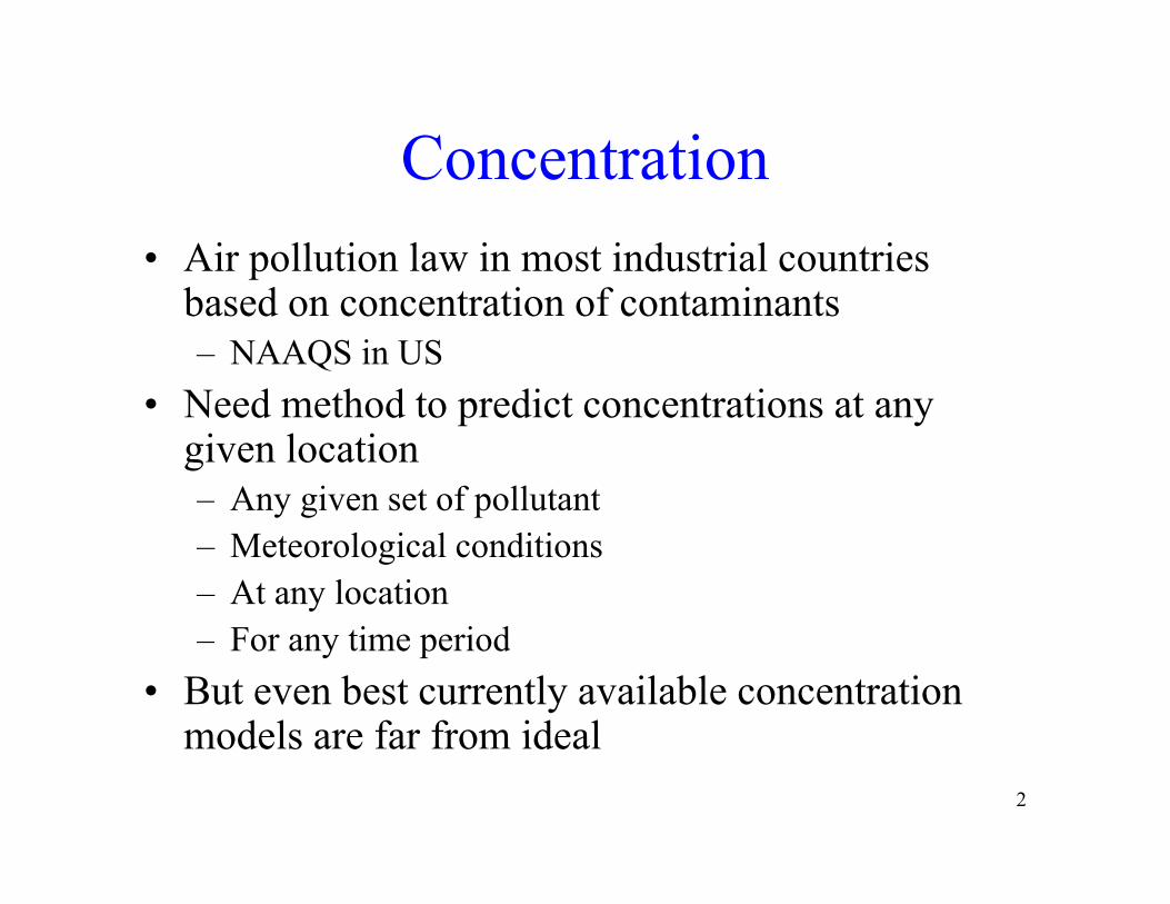
ConcentrationConcentration• Air pollution law in most industrial countries
based on concentration of contaminants– NAAQS in US
N d th d t di t t ti t• Need method to predict concentrations at any given location– Any given set of pollutantAny given set of pollutant– Meteorological conditions– At any location – For any time period
• But even best currently available concentration models are far from ideal
2
models are far from ideal

Concentration
• Commonly express concentration as ppm or μg/m3μg
• Parts per million (ppm) = 1 volume of 1 ppm = 1 volume gaseous pollutant– 1 ppm = __1 volume gaseous pollutant__
106 volumes (pollutant + air)/ 3 i / bi t• μg/m3 = micrograms/cubic meter
3

Factors that determine Dispersion
• Physical nature of effluents• Chemical nature of effluentsChemical nature of effluents• Meteorology
L i f h k• Location of the stack• Nature of terrain downwind from the stack
4

Stack EffluentsStack Effluents• Gas and particulate matter• Particles < 20 μm behave same as gas
– Low settling velocityP ti l > 20 h i ifi t ttli l it• Particle > 20 μm have significant settling velocity
• Only gases and Particles < 20 μm are treated in dispersion modelsdispersion models
• Others are treated as particulate matter• Assumes effluents leave the stack with sufficientAssumes effluents leave the stack with sufficient
momentum and buoyancy– Hot gases continue to rise
5
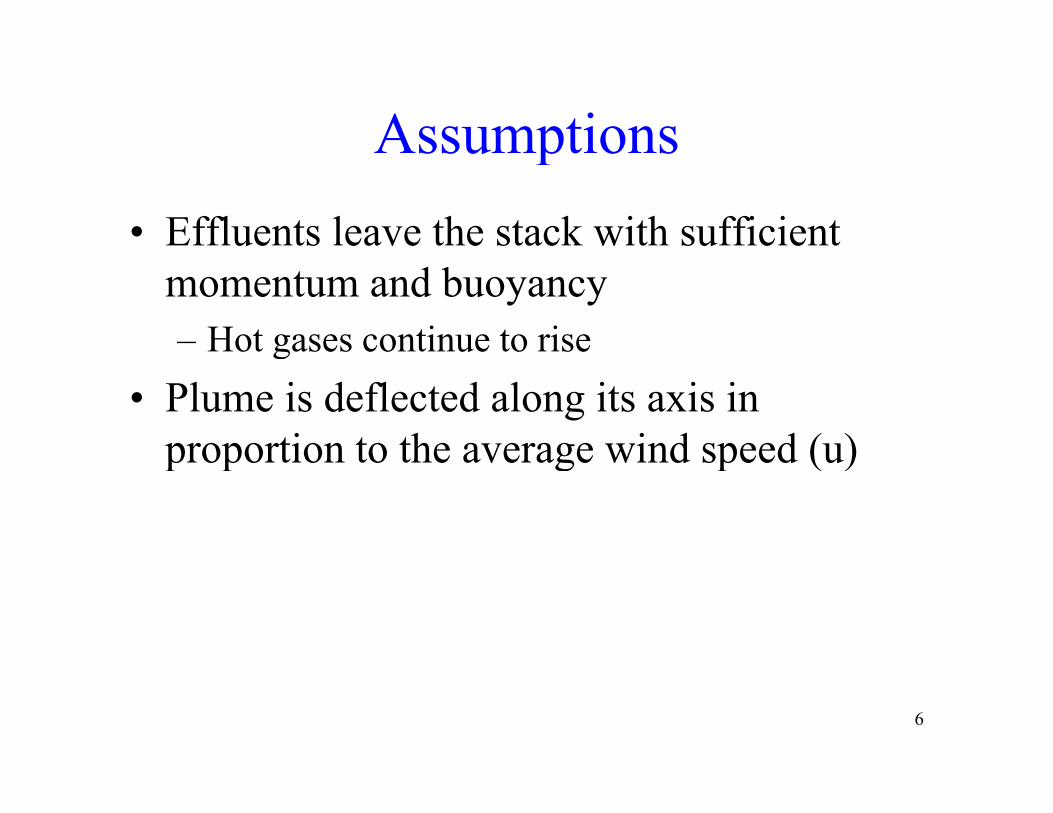
AssumptionsAssumptions• Effluents leave the stack with sufficient
momentum and buoyancy– Hot gases continue to riseg
• Plume is deflected along its axis in proportion to the average wind speed (u)proportion to the average wind speed (u)
6

Gaussian or Normal Distribution
• Gaussian distribution modelGaussian distribution model • Dispersion in y and z directions uses a
double gaussian distribution plumesdouble gaussian distribution -- plumes• Dispersion in (x, y, z) is three-dimensional• Used to model instantaneous puff of
emissions
7

Gaussian or Normal Distribution
• Pollution dispersion follows a distribution function
• Theoretical form: gaussian distribution functionfunction
8

Gaussian or Normal Distribution
• x = mean of the distributionx mean of the distribution• = standard deviationGaussian distribution used to model probabilities, in thisGaussian distribution used to model probabilities, in this context formula used to predict steady state concentration at a point down stream
9

Gaussian or Normal DistributionWhat are some properties of the normal distribution?distribution?
10f(x) becomes concentration, maximum at center of plume
Gaussian or Normal distribution
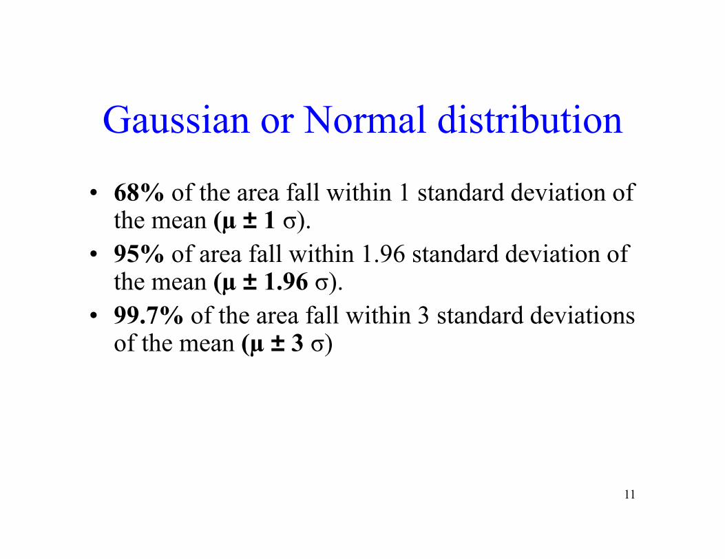
• 68% of the area fall within 1 standard deviation of the mean (µ ± 1 σ).
f f ll i hi d d d i i f• 95% of area fall within 1.96 standard deviation of the mean (µ ± 1.96 σ).
• 99 7% of the area fall within 3 standard deviations• 99.7% of the area fall within 3 standard deviations of the mean (µ ± 3 σ)
11

Gaussian dispersion model
• Dispersion in y and z directions are modeled as Gaussian
• Becomes double Gaussian model• Why doesn’t it follow a Gaussian• Why doesn t it follow a Gaussian
distribution in the x direction?Di ti f i d– Direction of wind
12

Gaussian Dispersion Model• For localized point sources – stacks• General appearance • Plume exits at height, hs• Rises an additional distance, Δh
– buoyancy of hot gases– buoyancy of hot gases– called plume rise– reaches distance where buoyancy and upward momentum cease
E it l it V• Exit velocity, Vs• Plume appears as a point source emitted at height H =
hs + Δh• Emission rate Q (g/s)• Assume wind blows in x direction at speed u
u is independent of time elevation or location (not really true)
13
– u is independent of time, elevation, or location (not really true)

Gaussian Dispersion Model
14
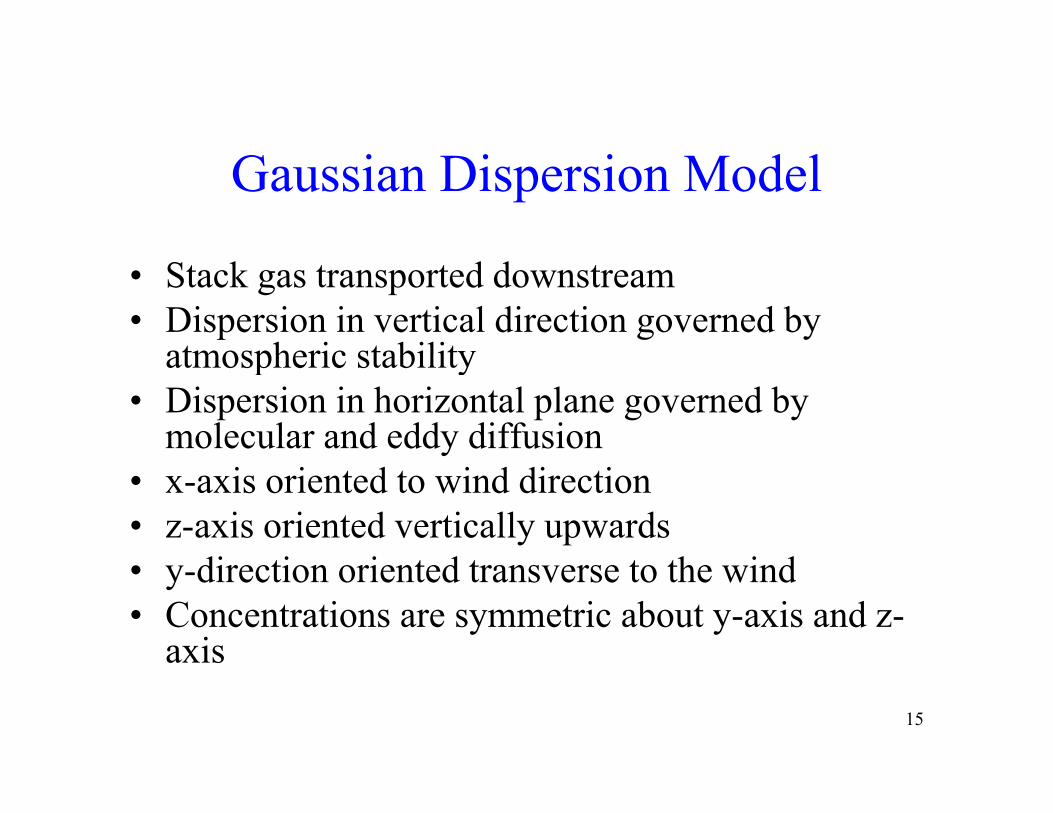
Gaussian Dispersion Model
• Stack gas transported downstream• Dispersion in vertical direction governed by
atmospheric stabilityatmospheric stability• Dispersion in horizontal plane governed by
molecular and eddy diffusion• x-axis oriented to wind direction• z-axis oriented vertically upwards
di ti i t d t t th i d• y-direction oriented transverse to the wind• Concentrations are symmetric about y-axis and z-
axis
15
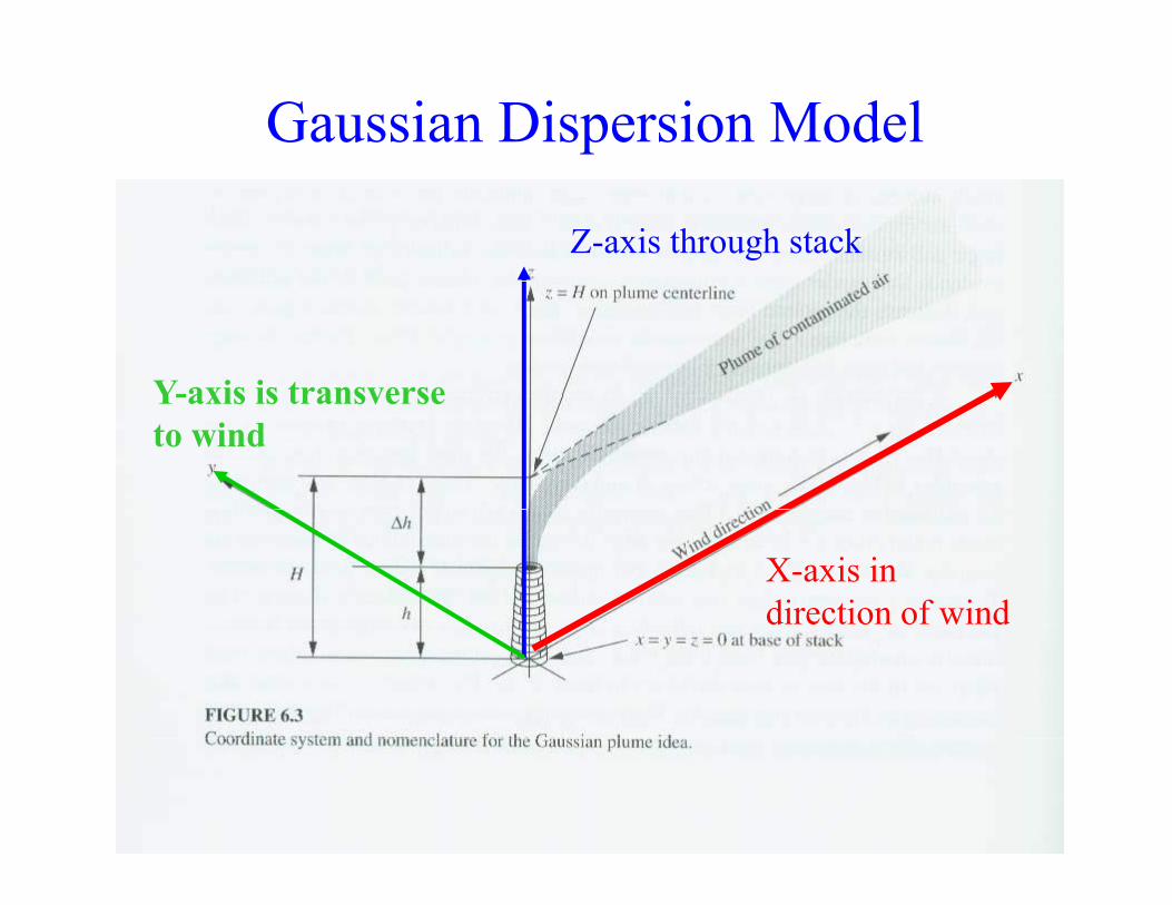
Gaussian Dispersion Model
Z-axis through stack
Y-axis is transverseY-axis is transverse to wind
X-axis in direction of winddirection of wind
16

As distanceAs distance increase so does dispersion
17Image source: Cooper and Alley, 2002

18Image source: Cooper and Alley, 2002

Point Source at Elevation H
• Assumes no interference or limitation to dispersion in any directiondispersion in any direction
d l i f li f lx0 and z0 are location of centerline of plumey0 taken as base of the stackz0 is HQ = emission strength of source (mass/time) – g/su = average wind speed thru the plume – m/sC = concentration – g/m3 (Notice this is not ppm)
19
y and z are horizontal and vertical standard deviations in meters

Wind Velocity ProfileWind Velocity Profile
• Wind speed varies by height• International standard height for wind-speed g p
measurements is 10 m• Dispersion of pollutant is a function of wind p p
speed at the height where pollution is emitted
• But difficult to develop relationship between height and wind speed
20

Point Source at Elevation H without Reflection
• 3 terms– gives concentration on the centerline of the plume– gives concentration as you move in the sideways direction ( y
2direction), direction doesn’t matter because ( y)2 gives a positive value
– gives concentration as you move in the vertical direction ( z direction) direction doesn’t matter because ( (z H))2 gives adirection), direction doesn t matter because ( (z – H))2 gives a positive value
• Concentrations are symmetric about y-axis and z-axis• Same concentration at (z-H) = 10 m as (z-H) =10 m
21
• Same concentration at (z-H) 10 m as (z-H) 10 m• Close to ground symmetry is disturbed

Point Source at elevation H withoutPoint Source at elevation H without reflection
• Equation 4-6 reduces to
Note in the book there are 2 equation 4-8s (2 different equations just labeled wrong)
22
(2 different equations just labeled wrong)
This is the first one
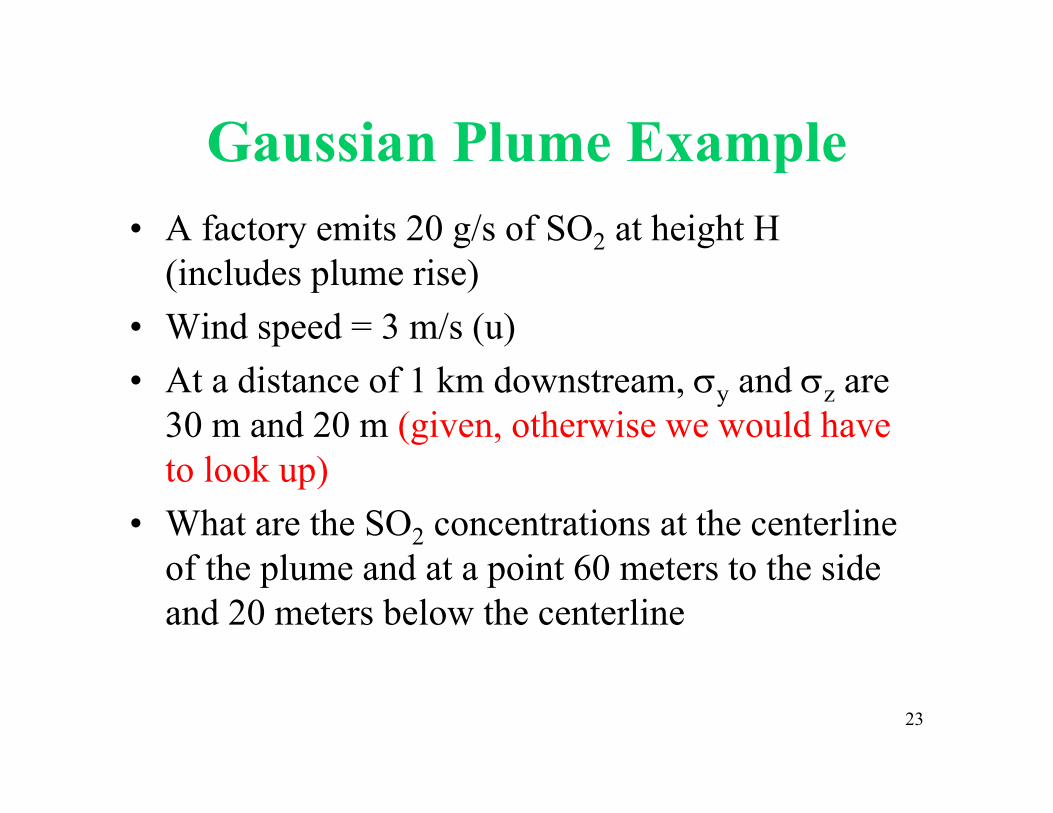
Gaussian Plume ExampleGaussian Plume Example• A factory emits 20 g/s of SO2 at height H
(includes plume rise)• Wind speed = 3 m/s (u)• At a distance of 1 km downstream, y and z are
30 m and 20 m (given, otherwise we would have l k )to look up)
• What are the SO2 concentrations at the centerline f th l d t i t 60 t t th idof the plume and at a point 60 meters to the side
and 20 meters below the centerline
23

Gaussian Plume Example0
• Q = 20 g/s of SO Z – H = 0 S d h lf• Q = 20 g/s of SO2
• u = 3 m/s (u)• y and z are 30 m and 20 m
So second half of equation goes to 0
• y = 0 and z = H• So reduces to:C(x,0,0) = 20 g/s = 0.00177 g/m3 = 1770 µ g/m3( , , ) __ g __ g µ g
2(Π*3*30*20)
24At centerline y and Z are 0

Gaussian Plume ExampleGaussian Plume ExampleWhat are the SO2 concentrations at a point 60 meters to the side and 20
meters below the centerlinemeters below the centerline
c = ____Q____ exp-1/2[(-y2) + ( (z-H)2)]2u y z [y
2 z2]
= ___20 g/s___ exp-1/2 [(-60m)2 + (-20m)2] =2 3*(30)(20) [(30m)2 (202m)]
(0.00177 g/m3) * (exp –2.5) = 0.000145 g/m3 or 145.23 µ g/m3
25At 20 and 60 meters

Evaluation of Standard Deviation
• Horizontal and vertical dispersion coefficients -- y z are a functiony z – downwind position x– Atmospheric stability conditionsAtmospheric stability conditions
• many experimental measurements –charts have been createdhave been created– Correlated y and z to atmospheric stability
and x26
and x

Pasquill-Gifford Curves
• Concentrations correspond to sampling times of approx. 10 minutes
• Regulatory models assume that the concentrations predicted represent 1-hour averages
• Solid curves represent rural values• Dashed lines represent urban values• Estimated concentrations represent only the lowest
several hundred meters of the atmosphere
27
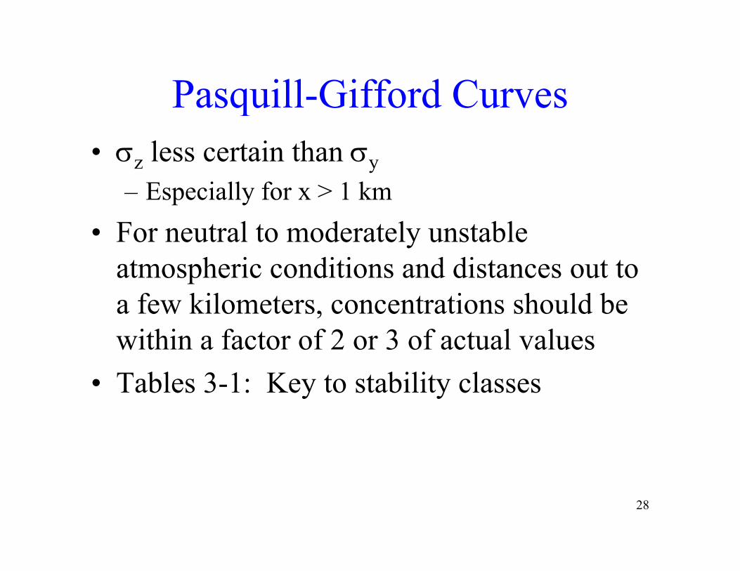
Pasquill-Gifford CurvesPasquill Gifford Curves• z less certain than y
– Especially for x > 1 km• For neutral to moderately unstable
atmospheric conditions and distances out to a few kilometers, concentrations should be within a factor of 2 or 3 of actual values
• Tables 3-1: Key to stability classesy y
28

ExampleFor stability class A, what are the values of y and z at 1 km downstream (assume urban)
From Tables 4-6 and 4-7From Tables 4 6 and 4 7
29

200
σy ~ 220 m
30

σz ~ 310 m
31
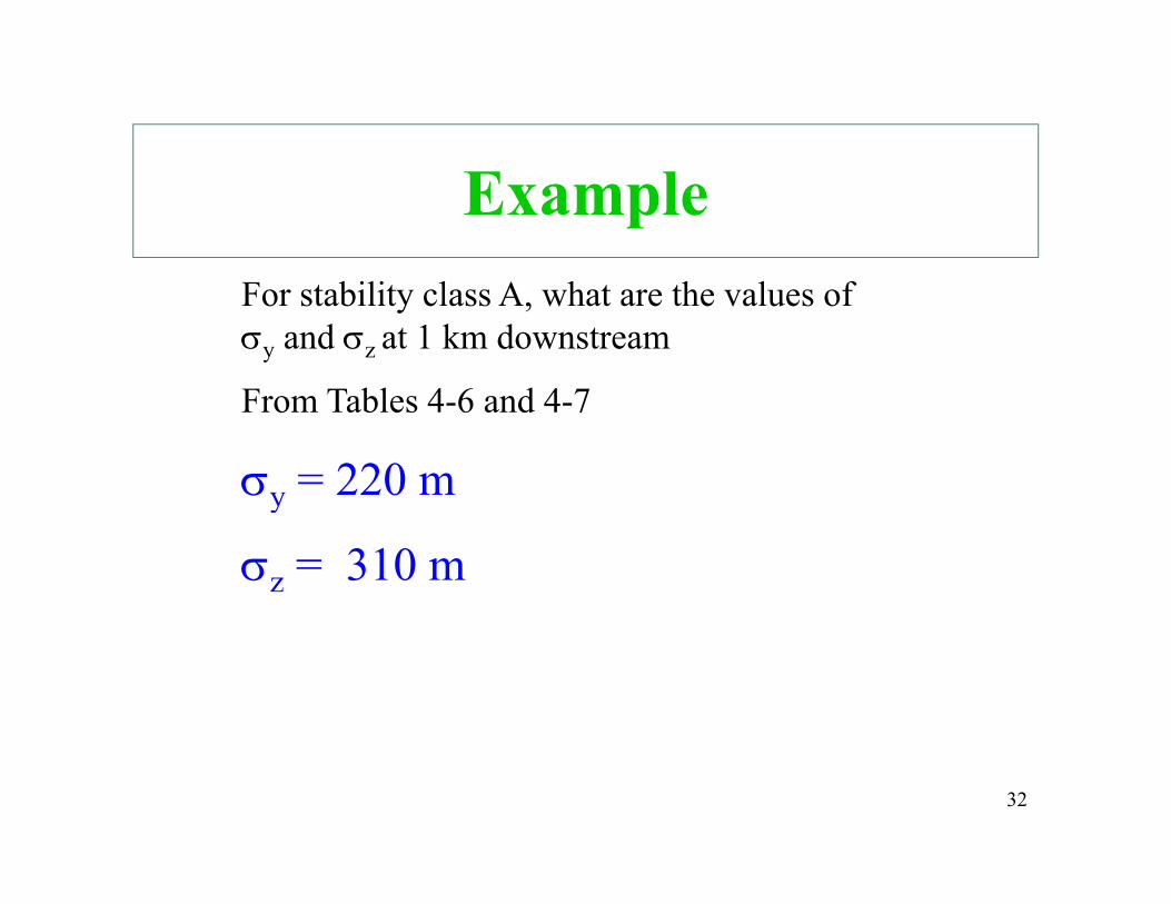
Examplebili l h h l fFor stability class A, what are the values of
y and z at 1 km downstream
F T bl 4 6 d 4 7From Tables 4-6 and 4-7
y = 220 my
z = 310 m
32

Empirical Equations
• Often difficult to read charts• Curves fit to empirical equationsp q
y = cxd
z = axbz
Where
d i d di t (kil t )x = downwind distance (kilometers)a, b, c, d = coefficients from Tables 4-1 and 4-2
33

E l h l f d 1 kExample: what are values of y and z at 1 km downstream for stability class A using equations rather than charts?y = cxd
z = axb
Using table 4-1 forUsing table 4 1 for stability class A
c = 24.1670d = 2.5334
34

Example: what are values of and at 1 kmExample: what are values of y and z at 1 km downstream for stability class A using equations rather than charts?
dy = cxd
z = axb
Using table 4-2 where x = 1 km
a = 453.850
b 2 11660b = 2.11660
35

Example: what are values of and at 1 km downstreamExample: what are values of y and z at 1 km downstream for stability class A using equations rather than charts?y = cxd
b a 453 850c 24 1670z = axb a = 453.850
b = 2.11660d = 2.5334c = 24.1670
Solutiony = cxd = 24.1670(1 km)2.5334 = 24.17 m = axb = 453 85(1 km)2.11660 = 453 9 mz ax 453.85(1 km) 453.9 m
36

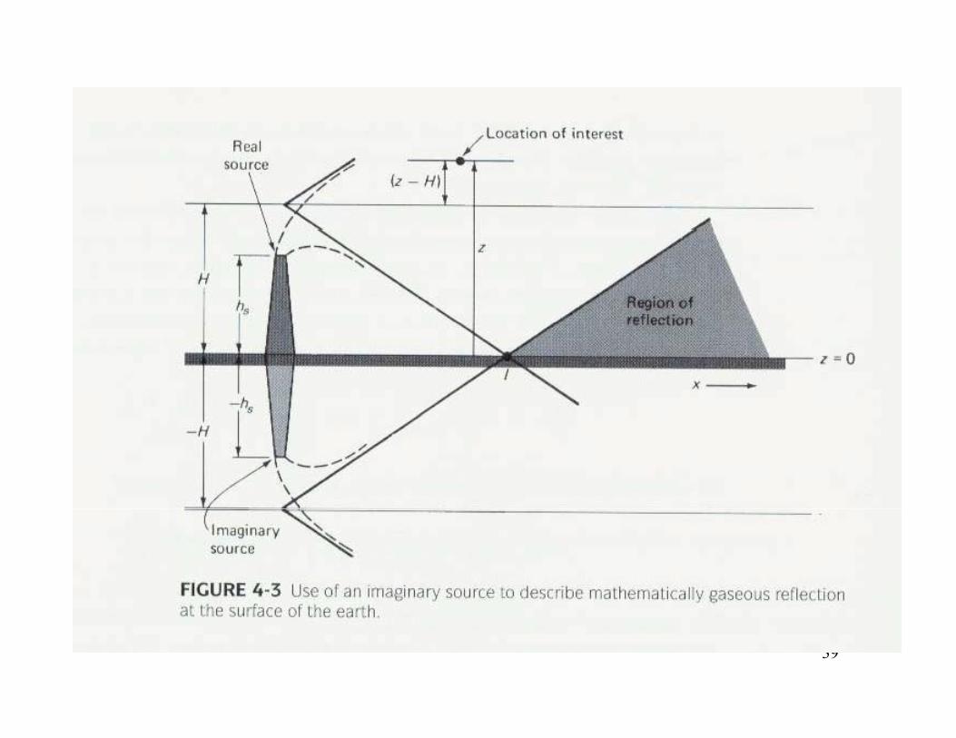
Point Source at Elevation H with Reflection
• Previous equation for concentration of plumes a considerable distance above pground
• Ground damps out vertical dispersionGround damps out vertical dispersion• Pollutants “reflect” back up from ground
37

Point Source at Elevation H with Reflection
• Accounts for reflection of gaseous• Accounts for reflection of gaseous pollutants back into the atmosphereR fl i di i• Reflection at some distance x is mathematically equivalent to having a
i i f h Hmirror image of the source at –H• Concentration is equal to contribution of
both plumes at ground level
38
39

Point Source at Elevation H with Reflection
Notice this is also equation 4-8 in text, it is the second equation 4-8 on theit is the second equation 4 8 on the bottom of page 149
40

Example: Point Source at Elevation H with ReflectionExample: Point Source at Elevation H with Reflection
Nitrogen dioxide is emitted at 110 g/s from stack with H = 80 m
Wind speed = 5 m/s
Plume rise is 20 m
Calculate ground level concentration 100 meter from centerline of plume (y)
41Assume stability class D so σy = 126 m and σz = 51 m

Example: Point Source at Elevation H with ReflectionExample: Point Source at Elevation H with Reflection
Q = 110 g/s H = 80 m u = 5 m/s Δh = 20 m y = 100 m
σ = 126 m and σ = 51 mσy = 126 m and σz = 51 m
Effective stack height =80 m + 20 m = 100 m
σy = 126 m and σz = 51 m
Solving in pieces 100 g/s = 0.000496
42
Solving in pieces _____100 g/s____ 0.000496
2Π*5*126*51

Example: Point Source at Elevation H with ReflectionExample: Point Source at Elevation H with Reflection
Q = 110 g/s H = 80 m u = 5 m/s Δh = 20 m y = 100 m
σ = 126 m and σ = 51 mσy = 126 m and σz = 51 m
Solving in pieces exp -[__1002 ] = 0.726149
[2*1252]
Solving in pieces exp -[ (0-100m)2 ] = 0.146265
43
Solving in pieces exp [ (0 100m) ] 0.146265
[2*512]

Example: Point Source at Elevation H with ReflectionExample: Point Source at Elevation H with Reflection
Q = 110 g/s H = 80 m u = 5 m/s Δh = 20 m y = 100 m
σ = 126 m and σ = 51 mσy = 126 m and σz = 51 m
Solving in pieces both sides of z portion are same so add
c = 0.000496 * 0.726149 * (2 * 0.14625) = 0.000116 g/m3 or 116.4 µg/m3
44
Ground Level Concentration withGround Level Concentration with reflection
• Often want ground level– People, property exposed to pollutantsPeople, property exposed to pollutants
• Previous eq. gives misleadingly low results near groundnear ground
• Pollutants “reflect” back up from ground
45

Ground Level ConcentrationGround Level Concentration• Equation for ground level concentration
1 1• Z = 0 1 1
Reduces to at ground level
1 + 1 cancels 2level
46

Ground Level ExampleC- stability classH = 50 mH 50 mQ = 95 g/sWind speed is 3 m/spWhat is ground level concentration at 0.5 km downwind,
along the centerline?From Figure 4-6, y = 90 m, From Figure 4-7, z = 32 m
C = 95 x 106 µg/s * exp[-(502)] exp [0] = 1023.3 µg/m3
(3 m/s)(90 m)(32 m) [ 2(32)2]47
(3 m/s)(90 m)(32 m) [ 2(32)2]

Maximum Ground LevelMaximum Ground Level Concentration
• Effect of ground reflection increases ground concentration
• Does not continue indefinitely• Eventually diffusion in y direction• Eventually diffusion in y-direction
(crosswind) and z-direction decreases concentrationconcentration
48

Maximum Ground LevelMaximum Ground Level Concentration
Values for a, b, c, d are in Table 4-5
49
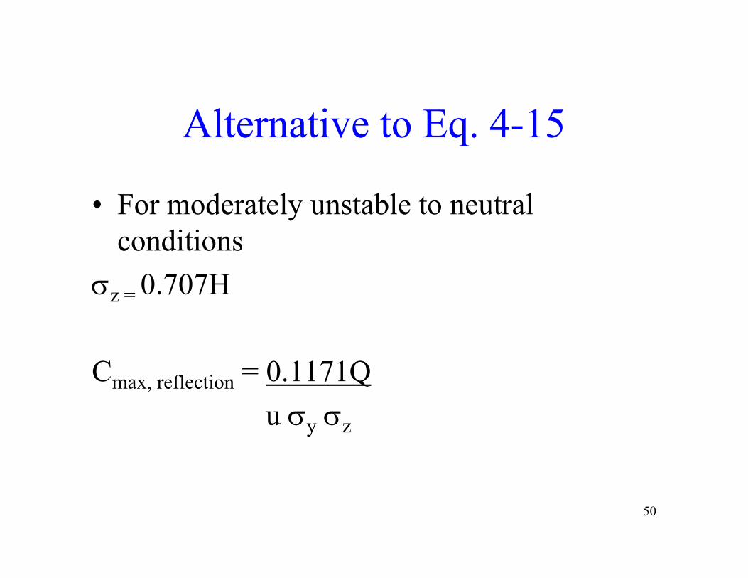
Alternative to Eq. 4-15
• For moderately unstable to neutral conditions
z = 0.707H
Cmax, reflection = 0.1171Qu y z
50

Max Concentration ExampleMax. Concentration ExampleWhat is maximum ground level concentration and where is it located downstream for the following?g•Wind speed = 2 m/s•H = 71 m•Stability Class B•Stability Class B•Q = 2,500,000 µg/s
S l iSolution:z = 0.707H = 0.707(71m) = 50.2 mFrom Figure 4-7, this occurs at x = 500 mg ,
51

z = 50.2 m
From Figure 4-7 thisFrom Figure 4-7, this occurs at x = 500 m
52
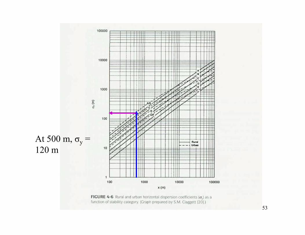
At 500 m, σy = 120 m
53

Max Concentration ExampleMax. Concentration ExampleWhat is maximum ground level concentration and where is it located downstream for the following?g•Wind speed = 2 m/s•H = 71 m•Stability Class B•Stability Class B•Q = 2,500,000 µg/s
S l iSolution:z = 0.707H = 0.707(71m) = 50.2 mFrom Figure 4-7, this occurs at x = 500 mg ,From Figure 4-6, y = 120 mCmax, reflection = 0.1171Q = 0.1171(2500000) = 24.3 µg/m3
54
u y z (2)(120)(50.2)

Calculation of Effective Stack Heightg
• H = hs + Δh• Δh depends on:Δh depends on:
– Stack characteristicsMeteorological conditions– Meteorological conditions
– Physical and chemical nature of effluentV i ti b d diff t• Various equations based on different characteristics, pages 162 to 166
55

Carson and Moses
• Equation 4-18
Where:Δh = plume rise (meters)Δh plume rise (meters)Vs = stack gas exit velocity (m/s)ds = stack exit diameter (meters)s ( )us = wind speed at stack exit (m/s)Qh = heat emission rate in kilojoules per second
56

Other basic equations
• Holland• concaweconcawe
57

Example:Example:
From text
H t i i t 4800 kj/Heat emission rate = 4800 kj/s
Wind speed = 5 mph
Stack gas velocity = 15 m/s
Stack diameter at top is 2 m
Estimate plume rise
58

Concentration Estimates for Different S li TiSampling Times
• Concentrations calculated in previous examples based on averages over 10 minute intervalson averages over 10-minute intervals
• Current regulatory applications use this as 1-hour average concentrationaverage concentration
• For other time periods adjust by:– 3-hr multiply 1-hr value by 0.9– 8-hr multiply 1-hr value by 0.7– 24-hr multiply 1-hr value by 0.4
l lti l 1 h l b 0 03 0 08– annual multiply 1-hr value by 0.03 – 0.08
59

Concentration Estimates for Different S li Ti E lSampling Times—Example
• For other time periods adjust by:3 h lti l 1 h l b 0 9– 3-hr multiply 1-hr value by 0.9
– 8-hr multiply 1-hr value by 0.7– 24-hr multiply 1-hr value by 0.4u t p y va ue by 0.– annual multiply 1-hr value by 0.03 – 0.08
Conversion of 1-hr concentration of previous example to an 8-hour average =
c8 hour = 36.4 µg/m3 x 0.7 = 25.5 µg/m38-hour µg µg
60
Line Sources
• Imagine that a line source, such as a highway, consists of an infinite number of g y,point sources
• The roadway can be broken into finiteThe roadway can be broken into finite elements, each representing a point source, and contributions from each element areand contributions from each element are summed to predict net concentration
61
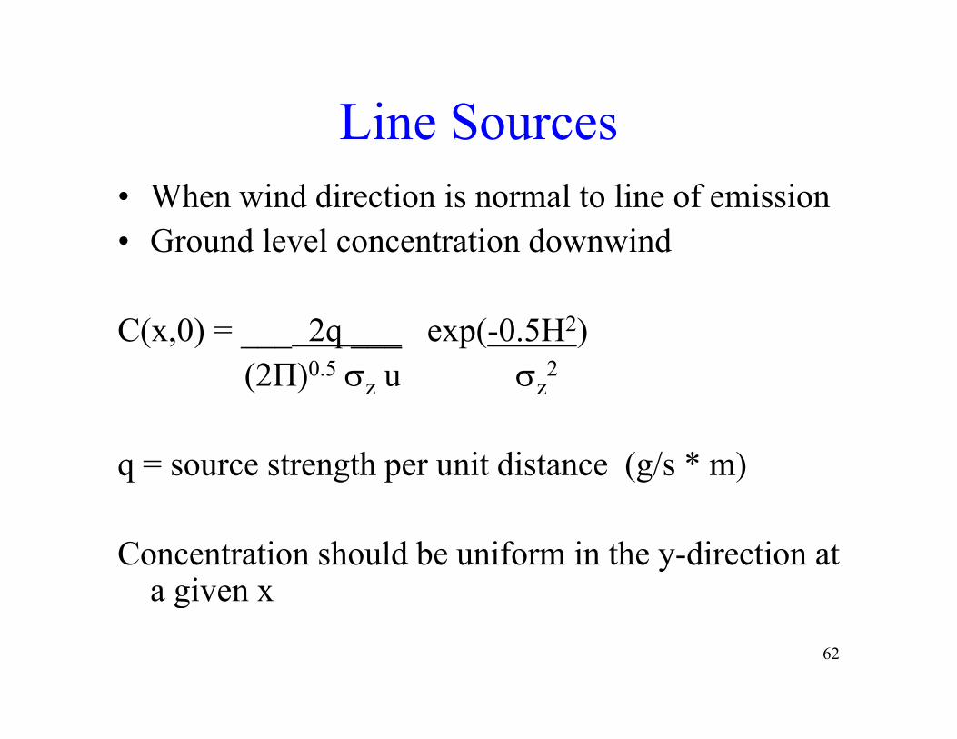
Line SourcesLine Sources• When wind direction is normal to line of emission
G d l l i d i d• Ground level concentration downwind
C( 0) 2 ( 0 5H2)C(x,0) = ___ 2q ___ exp(-0.5H2)(2Π)0.5 z u z
2
q = source strength per unit distance (g/s * m)
Concentration should be uniform in the y-direction at a given x
62
g

Line SourcesLine Sources• For ground level (H = 0), could also use breathing
heightheight
C(x 0) = 2q exp( 0 5H2)
1
C(x,0) = ___ 2q ___ exp(-0.5H )(2Π)0.5 z u z
2
63

Roadway Emissions and MixingRoadway Emissions and Mixing
64From Guensler, 2000u (wind direc

Instantaneous Release of a Puff• Pollutant released quickly
E l i• Explosion• Accidental spill• Release time << transport time• Also based on Gaussian distributionAlso based on Gaussian distribution
function
65

Instantaneous Release of a Puff• Equation 4-41 to predict maximum ground level q p g
concentration
Cmax = _____2Qp____(2Π)3/2 x y z
Receptor downwind would see a gradual increase in t ti til t f ff d d thconcentration until center of puff passed and then
concentration would decreaseAssume =
66
Assume x y

Figure 4-9 and Table 4-7
67

Figure 4-9 and Table 4-7
68

Puff ExampleA tanker spill on the freeway releases 400 000 grams of chlorineA tanker spill on the freeway releases 400,000 grams of chlorine. What exposure will vehicles directly behind the tanker (downwind) receive if x =100 m? Assume very stable conditions.
From Table 4-7,
69

Figure 4-9 and Table 4-7
70

Puff ExampleA tanker spill on the freeway releases 400 000 grams of chlorineA tanker spill on the freeway releases 400,000 grams of chlorine. What exposure will vehicles directly behind the tanker (downwind) receive if x =100 m? Assume very stable conditions.
From Table 4-7, y = 0.02(100m)0.89 = 1.21
F T bl 4 7 0 05(100 )0 61 0 83From Table 4-7, z = 0.05(100m)0.61 = 0.83
x = y = 1.21
71

Puff ExampleA tanker spill on the freeway releases 400 000 grams of chlorineA tanker spill on the freeway releases 400,000 grams of chlorine. What exposure will vehicles directly behind the tanker (downwind) receive if x =100 m? Assume very stable conditions.
From Table 4-7, y = 0.02(100m)0.89 = 1.21
F T bl 4 7 0 05(100 )0 61 0 83From Table 4-7, z = 0.05(100m)0.61 = 0.83
Cmax = _____2Qp____ = ____2(400000 g)_____ = 42,181 g/m3
(2Π)3/2 x y z (2Π)3/2(1.21)(1.21)(0.83)
72


