CERIAS Tech Report 2003-21
MULTICRITERIA ROUTING FOR GUARANTEED
PERFORMANCE COMMUNICATIONS
by Dong-won Shin
Center for Education and Research in Information Assurance and Security,
Purdue University, West Lafayette, IN 47909
MULTICRITERIA ROUTING FOR GUARANTEED PERFORMANCE
COMMUNICATIONS
A Thesis
Submitted to the Faculty
of
Purdue University
by
Dong-won Shin
In Partial Fulfillment of the
Requirements for the Degree
of
Doctor of Philosophy
August 2003

- ii -
To my wife, babies, and parents
for their unlimited support, encouragement, and love

- iii -
ACKNOWLEDGMENTS
I would like to express my sincere gratitude to my advisors Prof. E. K. P. Chong
and Prof. H. J. Siegel. It is my great fortune to work towards a Ph.D. under their
supervision. This thesis would not have been possible without them.
I thank all the professors who taught me in class or outside of class. Special
gratitude goes to Prof. N. B. Shroff for his special role as a co-chair of my doc-
toral committee. I also thank the other committee members Prof. A. Ghafoor and
Prof. S. Fahmy for their helpful comments. I am grateful to my officemates and many
other friends whose friendship has been a source of education and enjoyment.
Last in order but foremost in importance, I would like to thank my family for
their support, encouragement, and love. Special thanks are due to my wife Youn-a.
She was always with me over the difficult years at Purdue and CSU, and has become
the source of my passion in life.
My research was supported in part by the Purdue Center for Education and
Research in Information Assurance and Security (CERIAS), by the Colorado State
University George T. Abell Endowment, by DARPA/ISO under contracts DABT63-
99-C0010 and DABT63-99-C0012, and by NSF under grants ANI-0099137, ECS-
0098089, and ANI-0207892.
- iv -
TABLE OF CONTENTS
Page
LIST OF TABLES . . . . . . . . . . . . . . . . . . . . . . . . . . . . . . . . . vii
LIST OF FIGURES . . . . . . . . . . . . . . . . . . . . . . . . . . . . . . . . viii
ABSTRACT . . . . . . . . . . . . . . . . . . . . . . . . . . . . . . . . . . . . xi
1 Introduction . . . . . . . . . . . . . . . . . . . . . . . . . . . . . . . . . . . 1
1.1 Multicriteria routing . . . . . . . . . . . . . . . . . . . . . . . . . . . 1
1.2 Multiconstraint QoS routing . . . . . . . . . . . . . . . . . . . . . . . 3
1.3 Survivable multipath routing for WDM networks . . . . . . . . . . . 4
1.4 Organization and contributions . . . . . . . . . . . . . . . . . . . . . 5
2 Multiconstraint QoS Routing Using an Efficient Lookahead Method Basedon Link-State Protocols . . . . . . . . . . . . . . . . . . . . . . . . . . . . . 8
2.1 Introduction . . . . . . . . . . . . . . . . . . . . . . . . . . . . . . . . 8
2.2 Assumptions and definitions . . . . . . . . . . . . . . . . . . . . . . . 11
2.2.1 Multiconstraint QoS routing problem . . . . . . . . . . . . . . 11
2.2.2 Nonlinear path length . . . . . . . . . . . . . . . . . . . . . . 12
2.2.3 Eligibility test and lookahead method . . . . . . . . . . . . . . 13
2.3 Related work . . . . . . . . . . . . . . . . . . . . . . . . . . . . . . . 14
2.4 Elements of our approach . . . . . . . . . . . . . . . . . . . . . . . . 16
2.4.1 Multiple postpaths . . . . . . . . . . . . . . . . . . . . . . . . 16
2.4.2 Eligibility test of MPLMR . . . . . . . . . . . . . . . . . . . . 17
2.4.3 Lookahead method of MPLMR . . . . . . . . . . . . . . . . . 18
2.5 MPLMR: multi-postpath-based lookahead multiconstraint routing . . 20
2.5.1 MPLMR algorithm . . . . . . . . . . . . . . . . . . . . . . . . 20
2.5.2 Control variable r . . . . . . . . . . . . . . . . . . . . . . . . . 23
2.5.3 Comparison with competing schemes using an example . . . . 25
- v -
Page
2.5.4 Complexity of MPLMR . . . . . . . . . . . . . . . . . . . . . 28
2.6 Performance evaluation . . . . . . . . . . . . . . . . . . . . . . . . . . 29
2.6.1 Simulation setup . . . . . . . . . . . . . . . . . . . . . . . . . 29
2.6.2 Simulation results . . . . . . . . . . . . . . . . . . . . . . . . . 30
2.7 Conclusions . . . . . . . . . . . . . . . . . . . . . . . . . . . . . . . . 35
3 Distributed Multiconstraint QoS Routing Using a Depth-First SearchMethod Based on Distance-Vector Protocols . . . . . . . . . . . . . . . . . 37
3.1 Introduction . . . . . . . . . . . . . . . . . . . . . . . . . . . . . . . . 37
3.2 Assumptions and definitions . . . . . . . . . . . . . . . . . . . . . . . 39
3.3 Elements of our approach . . . . . . . . . . . . . . . . . . . . . . . . 40
3.3.1 Minimum normalized margin . . . . . . . . . . . . . . . . . . 40
3.3.2 Sequential path search . . . . . . . . . . . . . . . . . . . . . . 42
3.3.3 Depth-first search with limited crankbacks . . . . . . . . . . . 43
3.4 SPMP: single-prepath multi-postpaths . . . . . . . . . . . . . . . . . 46
3.4.1 SPMP algorithm . . . . . . . . . . . . . . . . . . . . . . . . . 46
3.4.2 Complexity of SPMP . . . . . . . . . . . . . . . . . . . . . . . 49
3.5 Performance evaluation . . . . . . . . . . . . . . . . . . . . . . . . . . 50
3.5.1 Generation of network topologies and QoS attribute values . . 50
3.5.2 Simulation results . . . . . . . . . . . . . . . . . . . . . . . . . 53
3.6 Conclusions . . . . . . . . . . . . . . . . . . . . . . . . . . . . . . . . 56
4 Survivable Multipath Routing Using Penalization Methods for WDM Networks 59
4.1 Introduction . . . . . . . . . . . . . . . . . . . . . . . . . . . . . . . . 59
4.2 Previous work . . . . . . . . . . . . . . . . . . . . . . . . . . . . . . . 62
4.3 Survivable multipath routing problem . . . . . . . . . . . . . . . . . . 64
4.3.1 Definitions and assumptions . . . . . . . . . . . . . . . . . . . 64
4.3.2 Problem formulation . . . . . . . . . . . . . . . . . . . . . . . 66
4.4 Elements of the proposed routing techniques . . . . . . . . . . . . . . 69
4.4.1 Link penalization . . . . . . . . . . . . . . . . . . . . . . . . . 69
- vi -
Page
4.4.2 Residual networks and link cancellation . . . . . . . . . . . . . 70
4.5 CPMR: conditional-penalization multipath routing . . . . . . . . . . 73
4.5.1 Two phases . . . . . . . . . . . . . . . . . . . . . . . . . . . . 73
4.5.2 Phase 1: no backup channels . . . . . . . . . . . . . . . . . . . 73
4.5.3 Phase 2: with backup channels . . . . . . . . . . . . . . . . . 74
4.5.4 Complexity of CPMR . . . . . . . . . . . . . . . . . . . . . . . 78
4.6 SPMR: successive-penalization multipath routing . . . . . . . . . . . 79
4.7 Performance evaluation . . . . . . . . . . . . . . . . . . . . . . . . . . 82
4.7.1 Performance metrics . . . . . . . . . . . . . . . . . . . . . . . 82
4.7.2 Upper bound . . . . . . . . . . . . . . . . . . . . . . . . . . . 82
4.7.3 Refining CPMR using simulated-annealing . . . . . . . . . . . 83
4.7.4 DPR: disjoint-paths routing . . . . . . . . . . . . . . . . . . . 86
4.7.5 Simulation setup . . . . . . . . . . . . . . . . . . . . . . . . . 87
4.7.6 Simulation results . . . . . . . . . . . . . . . . . . . . . . . . . 87
4.8 Conclusion . . . . . . . . . . . . . . . . . . . . . . . . . . . . . . . . . 94
5 Summary and Directions for Future Research . . . . . . . . . . . . . . . . . 96
LIST OF REFERENCES . . . . . . . . . . . . . . . . . . . . . . . . . . . . . 99
A Computation of the probability in (4.2) . . . . . . . . . . . . . . . . . . . . 104
B Computation of the penalty in (4.8) . . . . . . . . . . . . . . . . . . . . . . 106
VITA . . . . . . . . . . . . . . . . . . . . . . . . . . . . . . . . . . . . . . . . 107
- vii -
LIST OF TABLES
Table Page
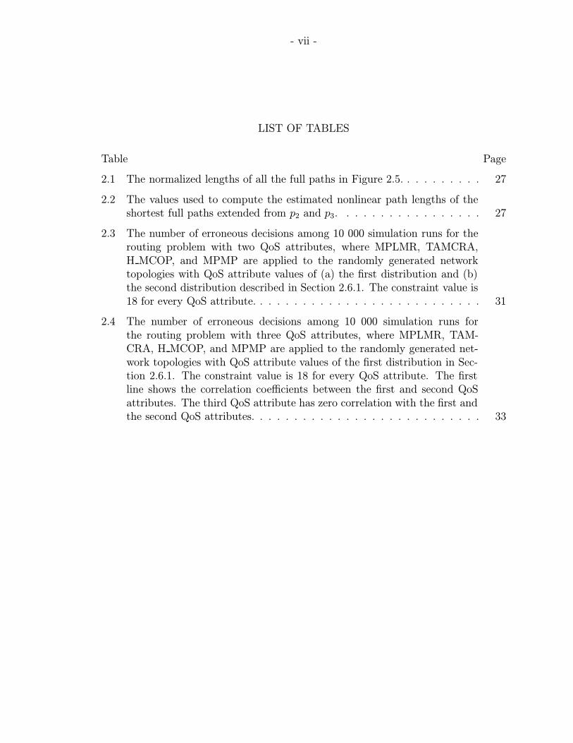
2.1 The normalized lengths of all the full paths in Figure 2.5. . . . . . . . . . 27
2.2 The values used to compute the estimated nonlinear path lengths of theshortest full paths extended from p2 and p3. . . . . . . . . . . . . . . . . 27
2.3 The number of erroneous decisions among 10 000 simulation runs for therouting problem with two QoS attributes, where MPLMR, TAMCRA,H MCOP, and MPMP are applied to the randomly generated networktopologies with QoS attribute values of (a) the first distribution and (b)the second distribution described in Section 2.6.1. The constraint value is18 for every QoS attribute. . . . . . . . . . . . . . . . . . . . . . . . . . . 31
2.4 The number of erroneous decisions among 10 000 simulation runs forthe routing problem with three QoS attributes, where MPLMR, TAM-CRA, H MCOP, and MPMP are applied to the randomly generated net-work topologies with QoS attribute values of the first distribution in Sec-tion 2.6.1. The constraint value is 18 for every QoS attribute. The firstline shows the correlation coefficients between the first and second QoSattributes. The third QoS attribute has zero correlation with the first andthe second QoS attributes. . . . . . . . . . . . . . . . . . . . . . . . . . . 33
- viii -
LIST OF FIGURES
Figure Page
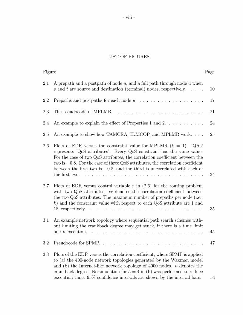
2.1 A prepath and a postpath of node u, and a full path through node u whens and t are source and destination (terminal) nodes, respectively. . . . . 10
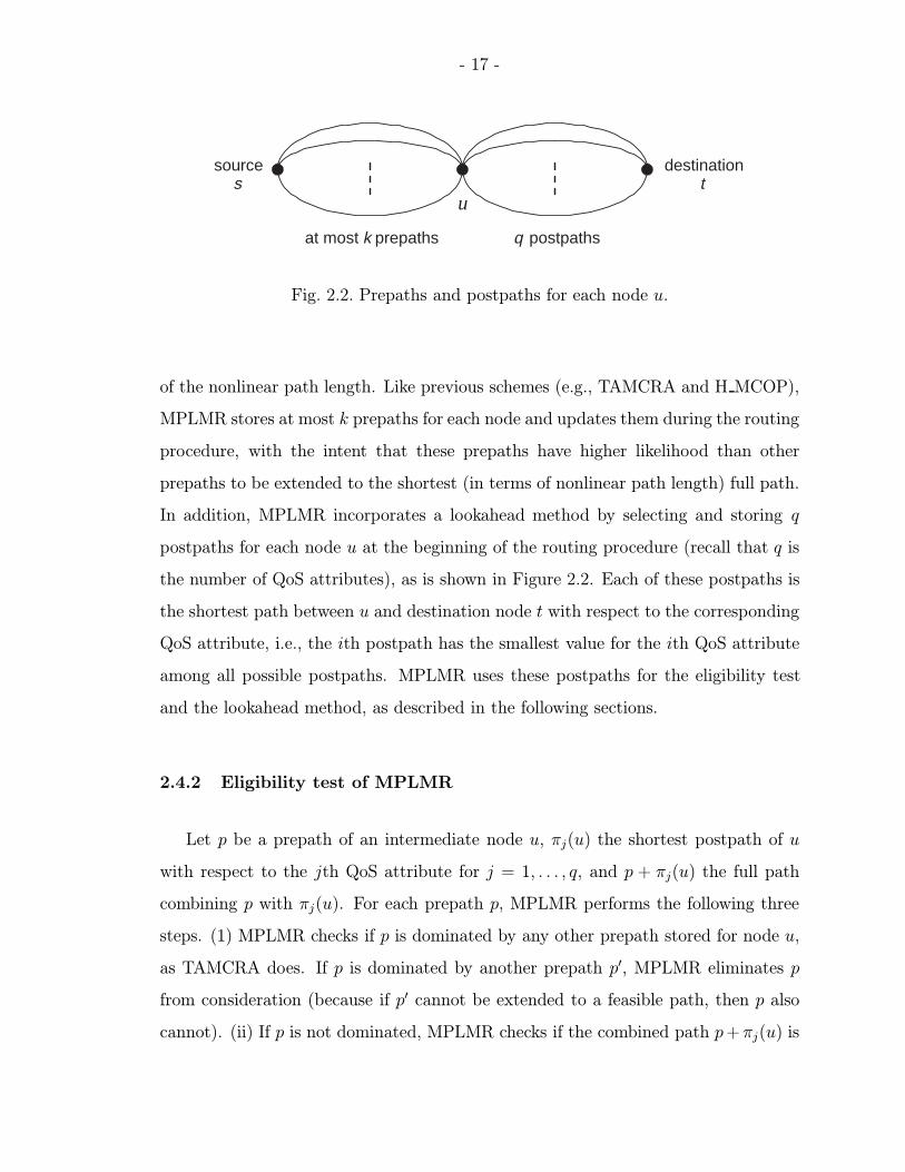
2.2 Prepaths and postpaths for each node u. . . . . . . . . . . . . . . . . . . 17
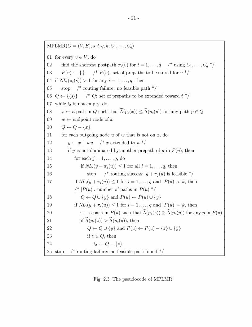
2.3 The pseudocode of MPLMR. . . . . . . . . . . . . . . . . . . . . . . . . 21
2.4 An example to explain the effect of Properties 1 and 2. . . . . . . . . . . 24
2.5 An example to show how TAMCRA, H MCOP, and MPLMR work. . . . 25
2.6 Plots of EDR versus the constraint value for MPLMR (k = 1). ‘QAs’represents ’QoS attributes’. Every QoS constraint has the same value.For the case of two QoS attributes, the correlation coefficient between thetwo is −0.8. For the case of three QoS attributes, the correlation coefficientbetween the first two is −0.8, and the third is uncorrelated with each ofthe first two. . . . . . . . . . . . . . . . . . . . . . . . . . . . . . . . . . 34
2.7 Plots of EDR versus control variable r in (2.6) for the routing problemwith two QoS attributes. cc denotes the correlation coefficient betweenthe two QoS attributes. The maximum number of prepaths per node (i.e.,k) and the constraint value with respect to each QoS attribute are 1 and18, respectively. . . . . . . . . . . . . . . . . . . . . . . . . . . . . . . . . 35
3.1 An example network topology where sequential path search schemes with-out limiting the crankback degree may get stuck, if there is a time limiton its execution. . . . . . . . . . . . . . . . . . . . . . . . . . . . . . . . 45
3.2 Pseudocode for SPMP. . . . . . . . . . . . . . . . . . . . . . . . . . . . . 47
3.3 Plots of the EDR versus the correlation coefficient, where SPMP is appliedto (a) the 400-node network topologies generated by the Waxman modeland (b) the Internet-like network topology of 4000 nodes. h denotes thecrankback degree. No simulation for h = 4 in (b) was performed to reduceexecution time. 95% confidence intervals are shown by the interval bars. 54
- ix -
Figure Page
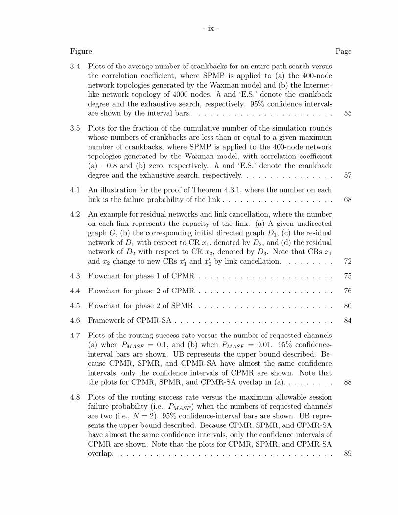
3.4 Plots of the average number of crankbacks for an entire path search versusthe correlation coefficient, where SPMP is applied to (a) the 400-nodenetwork topologies generated by the Waxman model and (b) the Internet-like network topology of 4000 nodes. h and ‘E.S.’ denote the crankbackdegree and the exhaustive search, respectively. 95% confidence intervalsare shown by the interval bars. . . . . . . . . . . . . . . . . . . . . . . . 55
3.5 Plots for the fraction of the cumulative number of the simulation roundswhose numbers of crankbacks are less than or equal to a given maximumnumber of crankbacks, where SPMP is applied to the 400-node networktopologies generated by the Waxman model, with correlation coefficient(a) −0.8 and (b) zero, respectively. h and ‘E.S.’ denote the crankbackdegree and the exhaustive search, respectively. . . . . . . . . . . . . . . . 57
4.1 An illustration for the proof of Theorem 4.3.1, where the number on eachlink is the failure probability of the link . . . . . . . . . . . . . . . . . . . 68
4.2 An example for residual networks and link cancellation, where the numberon each link represents the capacity of the link. (a) A given undirectedgraph G, (b) the corresponding initial directed graph D1, (c) the residualnetwork of D1 with respect to CR x1, denoted by D2, and (d) the residualnetwork of D2 with respect to CR x2, denoted by D3. Note that CRs x1
and x2 change to new CRs x′1 and x′2 by link cancellation. . . . . . . . . 72
4.3 Flowchart for phase 1 of CPMR . . . . . . . . . . . . . . . . . . . . . . . 75
4.4 Flowchart for phase 2 of CPMR . . . . . . . . . . . . . . . . . . . . . . . 76
4.5 Flowchart for phase 2 of SPMR . . . . . . . . . . . . . . . . . . . . . . . 80
4.6 Framework of CPMR-SA . . . . . . . . . . . . . . . . . . . . . . . . . . . 84
4.7 Plots of the routing success rate versus the number of requested channels(a) when PMASF = 0.1, and (b) when PMASF = 0.01. 95% confidence-interval bars are shown. UB represents the upper bound described. Be-cause CPMR, SPMR, and CPMR-SA have almost the same confidenceintervals, only the confidence intervals of CPMR are shown. Note thatthe plots for CPMR, SPMR, and CPMR-SA overlap in (a). . . . . . . . . 88
4.8 Plots of the routing success rate versus the maximum allowable sessionfailure probability (i.e., PMASF ) when the numbers of requested channelsare two (i.e., N = 2). 95% confidence-interval bars are shown. UB repre-sents the upper bound described. Because CPMR, SPMR, and CPMR-SAhave almost the same confidence intervals, only the confidence intervals ofCPMR are shown. Note that the plots for CPMR, SPMR, and CPMR-SAoverlap. . . . . . . . . . . . . . . . . . . . . . . . . . . . . . . . . . . . . 89
- x -
Figure Page
4.9 Plots of the average number of channels in a realized session versus thenumber of requested channels (a) when PMASF = 0.1, and (b) whenPMASF = 0.01. 95% confidence-interval bars are shown. Because CPMRand CPMR-SA have almost the same confidence intervals, only the con-fidence intervals of CPMR are shown. Note that the plots for CPMR,SPMR, and CPMR-SA overlap in (a), and the plots for CPMR and CPMR-SA overlap in (b). . . . . . . . . . . . . . . . . . . . . . . . . . . . . . . . 91
4.10 Plots of the average number links on a CR versus the number of requestedchannels (a) when PMASF = 0.1, and (b) when PMASF = 0.01. 95%confidence-interval bars are shown. Because the widths of confidence in-tervals are almost the same for all the schemes, only the confidence inter-vals of CPMR are shown. Note that the plots for CPMR and CPMR-SAoverlap in (a) and (b). . . . . . . . . . . . . . . . . . . . . . . . . . . . . 92
4.11 Plots of the number of terminations of the search procedure (using thesimulated annealing algorithm) in CPMR-SA by stopping criteria (A) and(B), (a) when PMASF = 0.1, and (b) when PMASF = 0.01. SC-(A) andSC-(B) denote the stopping criteria (A) and (B), respectively. . . . . . . 93
- xi -
ABSTRACT
Shin, Dong-won. Ph.D., Purdue University, August, 2003. Multicriteria routing forguaranteed performance communications. Major Professors: E. K. P. Chong andH. J. Siegel.
In this thesis, we investigate two routing problems. The first, which is known as
the multiconstraint QoS (quality of service) routing problem, is to find a single path
that satisfies multiple QoS constraints. For this problem, we consider two routing
environments: (a) a given source node has detailed routing information provided by
a link-state protocol, and (b) the source node has relatively simple routing infor-
mation provided by a distance-vector protocol. First, we develop a greedy scheme,
called MPLMR (multi-postpath-based lookahead multiconstraint routing), for case
(a). MPLMR has an efficient “look-ahead” feature that uses the detailed informa-
tion provided by link-state protocols. MPLMR has significantly better performance
than competing schemes in the literature. We then develop a sequential path-search
scheme, called SPMP (single-prepath multi-postpaths), for case (b). SPMP performs
routing with simple routing information provided by distance-vector protocols, and
maintains a small number of nodes involved in routing process. Hence, SPMP is
suitable for multiconstraint QoS routing in the situations where reduction in compu-
tational/signaling overhead is a concern.
The second problem that we deal with in this thesis is to find a minimum num-
ber of paths that can collectively satisfy constraints on channel demand, capacity,
and survivability between a given pair of source and destination nodes in a WDM
(wavelength division multiplexing) network. Different from previous survivable rout-
ing schemes for WDM networks, we introduce link failure probabilities to the prob-
lem. Because this routing problem is NP-hard, we develop heuristic multipath routing
schemes: CPMR (conditional-penalization multipath routing) and SPMR (successive-
- xii -
penalization multipath routing). These schemes allow each link to be used for several
channels. To deal with the difficulty that this link-sharing causes, we develop “link
penalization” methods to control link-sharing. CPMR takes a long run-time to find a
near-optimal solution, while SPMR uses a simple penalization method to reduce the
run-time at the slight expense of the routing success rate. Via simulation, we show
that our schemes achieve near-optimal routing success rates.
- 1 -
1. INTRODUCTION
1.1 Multicriteria routing
The goal of routing in computer/communication networks is to set up a routing
path or paths between source and destination (terminal) nodes to forward user traffic
in accordance with user requirements and network restrictions. Multicriteria routing
refers to the process of finding a path or paths satisfying multiple criteria (e.g., objec-
tives and constraints), which are set by such requirements and restrictions. Although
routing for various requirements and restrictions has been studied for a long time, it
is still an active area of research and development. User requirements for high-quality
services and the evolution of networking technologies constantly reveal opportunities
for the research and development of new routing schemes.
In this thesis, we deal with two routing problems. The first problem is to find a
single path that satisfies multiple QoS (quality of service) constraints. This problem is
known as the multiconstraint QoS routing problem, and has been receiving significant
attention. The second problem is to find a minimum number of paths that can
collectively satisfy constraints between a given pair of source and destination nodes
in a WDM (wavelength division multiplexing) network. For this problem, we consider
the constraints on channel demand, capacity, and survivability. Note that the first and
second problems focus on multiconstraint routing and multipath routing, respectively.
Both problems are NP-hard, and thus we develop heuristic schemes to solve these
problems in efficient manners.
Typically, routing schemes consist of two components: information advertise-
ment and path search. Information advertisement represents the periodical or event-
triggering dissemination of routing information to be used for path search. Path
- 2 -
search represents the computation or examination to find a path or paths to achieve
a given objective, while satisfying given constraints.
For information advertisement, there are two kinds of protocols: link-state proto-
cols [Moy95] and distance-vector protocols [MaS95]. If a link-state protocol is used
for information advertisement, each node u distributes to all other nodes the detailed
information on the links between u and its neighboring nodes. Thus, the control
message overhead for information advertisement is large in routing schemes based on
link-state protocols. However, information advertisement using a link-state protocol
is advantageous for path search, in the sense that routing paths can be computed
using detailed link-state information.
In contrast, if a distance-vector protocol is used, each node u is provided the
following information from each neighboring node v: the estimated value of the “best”
(with respect to each of the attributes considered) path between v and every possible
destination node. Node u estimates and updates the value of the best path to every
possible destination node with respect to each attribute, using the estimates obtained
from its neighboring nodes and the corresponding values of the links between u and
the neighboring nodes. Because each node exchanges estimated values only with its
neighboring nodes, distance-vector protocols have smaller signaling overhead than
that of link-state protocols for the distribution of routing information.
Depending not only on given constraints but also on the protocol used for informa-
tion advertisement, path search in multiconstraint routing may cause heavy signaling
overhead or require intensive computation. In this thesis, we focus on path search,
with the assumption that a protocol for information advertisement is given. For the
first problem, we develop two routing schemes based on link-state and distance-vector
protocols, respectively. For the second problem, we assume that a link-state proto-
col is used, and develop two routing schemes with characteristics different from each
other.
- 3 -
1.2 Multiconstraint QoS routing
The notion of QoS has been proposed for the qualitatively or quantitatively defined
performance contract between a service provider and a user. The QoS requirements
of a user for a connection impose a set of constraints for routing. Multiconstraint
QoS routing is to find a path satisfying the QoS constraints between given source and
destination nodes, called a feasible path. The optimization of resource utilization is
often considered additionally (e.g., [ChN98b,FeM02,KoK01,LiR01]).
Multiconstraint QoS routing is an essential mechanism to support future high-
quality multimedia services. A great number of multiconstraint QoS routing schemes
have been proposed for specific routing problems (e.g., the scheme in [WaC96] for
routing problems with limitations on bandwidth and delay). However, in this thesis,
we deal with “general” multiconstraint QoS routing schemes, which can be applied
to routing problems with any QoS constraints.
We can classify multiconstraint QoS routing schemes into unicast routing schemes
and multicast routing schemes, according to the number of destination nodes involved.
Unicast routing schemes search for a feasible path between a single pair of source
and destination nodes (e.g., [CuX03, GhS01, MaS97, KoK01, NeM00]). In contrast,
multicast routing schemes search for a feasible tree covering a single source node and
a set of destination nodes (e.g., [RoB02, RoB97, WuH00]). In this thesis, we limit
ourselves to unicast routing schemes.
We can also classify multiconstraint QoS routing schemes into source routing
schemes and distributed routing schemes, according to how many nodes in a given
network participate in path search. In source routing schemes (e.g., [ChN98a, Jaf84,
KoK01,NeM00,Yua02]), the source node computes a routing path using global state
information (i.e., the routing information of all the nodes and links in the network),
which is typically provided by a link-state protocol. Because of the local computation
by the source node, source routing schemes are conceptually simple and easy to
implement, maintain, and upgrade. In contrast, in distributed routing schemes (e.g.,
- 4 -
[GhS01, ShC95, SoP00, WaC96]), the path-search process is distributed among the
nodes between source and destination nodes. Hence, the computational overhead at
each node is relatively low, and thus distributed routing schemes are more scalable
than source routing schemes.
We can further classify distributed routing schemes into two groups, according to
how the routing information of a given network is maintained: distributed routing
schemes using global state information and distributed routing schemes using local
state information only. The global state information is provided by link-state or
distance-vector routing protocols used for information advertisement. Distributed
routing schemes using global state information have several features similar to those
of source routing schemes because of the same information-advertisement process.
In contrast, distributed routing schemes using local state information do not need
information advertisement. However, these schemes have the drawback of heavy
message overhead during the path-search procedure, because a large number of copies
of a given connection request must be forwarded to find a feasible path. We limit
our interest to routing schemes that can be implemented as source routing schemes
or distributed routing schemes using global state information.
1.3 Survivable multipath routing for WDM networks
By aggregating wavelength channels onto a fiber, wavelength division multiplexing
(WDM) makes it possible to use the large bandwidth of a fiber for a number of
connections without the need for high-speed optoelectronic devices. It is clear that
WDM networks will play an important role in the high-capacity telecommunication
world. Kotelly [Kot96] pointed out that all major long-distance carriers in the United
States have already used point-to-point WDM transmission technologies, and that
wavelength routing will be introduced in most carrier networks in the world soon.
As the number of channels accommodated on a fiber increases, the following prob-
lem becomes more critical: even a single link failure may lead to the loss of many
- 5 -
end-to-end connections. Hence, survivability is indispensable in WDM networks.
Moreover, as WDM transmission technologies are used more widely in current point-
to-point networks, the dynamic establishment of channel demands becomes more
important. In this thesis, we deal with the routing problem of finding a set of paths
between a pair of source and destination nodes on a given physical network topol-
ogy such that the paths accommodate the requested channels without violating given
constraints, including the constraint on survivability. To develop routing schemes for
this problem, we assume that the routing information associated with each link in
the network is provided to the source node by a link-state protocol.
Survivable routing schemes can be categorized into two groups: restoration
schemes (also known as dynamic or reactive schemes) and protection schemes (also
known as preplanned or proactive schemes) [Ban99, HwA01, Kya98, RaM99, ZaO03].
Restoration schemes do not reserve redundant resources for backup channels. Instead,
when failures occur, they search for available channels to reroute the connections of
affected channels. In contrast, protection schemes reserve backup channels in advance
so that in the event of failure the backup channels replace the affected channels. Pro-
tection schemes not only guarantee communication restoration, but also minimize the
duration and range of failure impact. These features of protection schemes are highly
desirable for networks that require high reliability. We limit our interest to protection
schemes in this thesis.
1.4 Organization and contributions
The organization and contributions of this thesis are as follows.
Chapter 2: In this chapter, we develop a multiconstraint QoS routing scheme,
called MPLMR (multi-postpath-based lookahead multiconstraint routing), with the
assumption that a link-state protocol is used for information advertisement. MPLMR
uses an extended version of a standard (single-constraint) shortest-path algorithm
with the notion of the nonlinear path length. Like previous schemes using extended
- 6 -
shortest-path algorithms for polynomial complexity, MPLMR stores a limited number
of subpaths between the source node and each intermediate node, and extends these
subpaths toward the destination node. However, MPLMR uses an improved “look-
ahead” method to predict the path length of the full path to which each subpath
is extended. MPLMR then selects and stores the subpaths that have higher likeli-
hood than other subpaths to be extended to feasible paths. We show via simulation
that MPLMR has a significantly smaller probability of missing a feasible path than
competing schemes in the literature.
Chapter 3: In this chapter, we propose another multiconstraint QoS routing
scheme, called SPMP (single-prepath multi-postpaths). Different from most previous
multiconstraint QoS routing schemes and MPLMR, SPMP assumes that a distance-
vector protocol is used for information advertisement. Moreover, SPMP minimizes
the number of nodes involved in the routing process by taking a sequential path-
search approach. Hence, SPMP is a multiconstraint QoS routing scheme that is
appropriate for a routing environment where the signaling overhead must be reduced.
Via simulation, we show that SPMP has low average-case time complexity.
Chapter 4: Most previous protection schemes for WDM networks assume that
the maximum number of simultaneous link failures is known (e.g., at most a single
link failure), and search for link-disjoint paths based on this assumption. However,
we take an alternative approach by introducing link failure probabilities to the rout-
ing problem, to develop routing schemes based on more general assumptions. In
this chapter, we propose two survivable multipath routing schemes for WDM net-
works: CPMR (conditional-penalization multipath routing) and SPMR (successive-
penalization multipath routing). These schemes allow each link to be used for several
channels. To deal with the difficulty that this link-sharing causes, we develop “link
penalization” methods to control link-sharing. CPMR takes a long run-time to find a
near-optimal solution, while SPMR uses a simple penalization method to reduce the
run-time at the slight expense of the routing success rate. We show via simulation

- 7 -
that our schemes have significantly higher routing success rates than a routing scheme
that searches for disjoint paths.
Chapter 5: We summarize the important results of this thesis, and discuss some
directions for future research.
- 8 -
2. MULTICONSTRAINT QOS ROUTING USING AN
EFFICIENT LOOKAHEAD METHOD BASED ON
LINK-STATE PROTOCOLS
2.1 Introduction
In this chapter, we deal with the multiconstraint QoS routing problem that
searches for a feasible path between a single pair of source and destination nodes.
We assume that a link-state protocol is used for the advertisement of routing infor-
mation. Hence, detailed routing information (i.e., the topology of a given network
and QoS attribute values of every link) is assumed to be avaliable for path search.
However, this multiconstraint QoS routing problem is NP-complete [Wan99], and
thus we need heuristic schemes to solve this problem within a limited time. Because
heuristic schemes may fail to find an existing solution, typical performance measures
for multiconstraint QoS routing schemes are time/memory complexity and erroneous
decision rate (EDR). The EDR is defined as the fraction of instances that a routing
scheme either fails to find a feasible path that exists, or finds a path that turns out
to be infeasible. Low complexity and low EDR are the main goals of multiconstraint
QoS routing schemes.
Every QoS attribute to be considered in multiconstraint QoS routing is either
a min/max attribute or a cumulative attribute (i.e., an additive attribute and a
multiplicative attribute in [Wan99]). A min/max attribute is a QoS attribute whose
value for a path is the minimum/maximum value of that QoS attribute for any link
on the path. In contrast, a cumulative attribute is a QoS attribute whose value for a
path is the sum or product of that QoS attribute for all the links on the path. Because
QoS attribute values of every link are known, min/max attributes (e.g., bandwidth)
can be dealt with easily by pruning all links (and possibly their incident nodes) that
- 9 -
do not satisfy the constraints on the attributes before starting to search for a feasible
path [WaC96]. Multiplicative QoS attributes can be regarded as additive by taking
logarithms. Therefore, it suffices to consider only additive QoS attributes for the
multiconstraint QoS routing problem. Hence, the constraint values are the maximum
values that the QoS attributes of a routing path must not exceed.
Because of the additivity of QoS attributes considered, the value of a path with
respect to a QoS attribute can be regarded as the “length” of the path with respect
to the QoS attribute. If a QoS routing problem has only one QoS attribute consid-
ered, then the single-constraint QoS routing problem can be solved using a standard
shortest-path algorithm (e.g., Dijkstra’s algorithm or the Bellman-Ford algorithm).
It is easy to see that the single-constraint QoS routing problem has a feasible solution
if and only if the shortest path between the source and destination nodes is feasible.
To solve the multiconstraint QoS routing problem in the same way, several schemes
take the approach that uses extended versions of a standard shortest-path algorithm,
which we call extended shortest path algorithms in this chapter. However, these
schemes must use a modified definition of length, because the “length” in the mul-
ticonstraint QoS routing problem cannot be defined as in the single-constraint QoS
routing problem. Unfortunately, for the modified definitions of length, the multicon-
straint QoS routing problem has the following property: The shortest path between
the source node and an arbitrary node u may not be a subpath of the shortest path
between the source and destination nodes through u. Hence, to find the shortest path
between the source and destination nodes, we may have to store all the subpaths
between the source node and each intermediate node during the routing procedure,
extend them to the destination node, and compare all the paths between the source
and destination nodes at the end. Unfortunately, this path search has exponential
complexity.
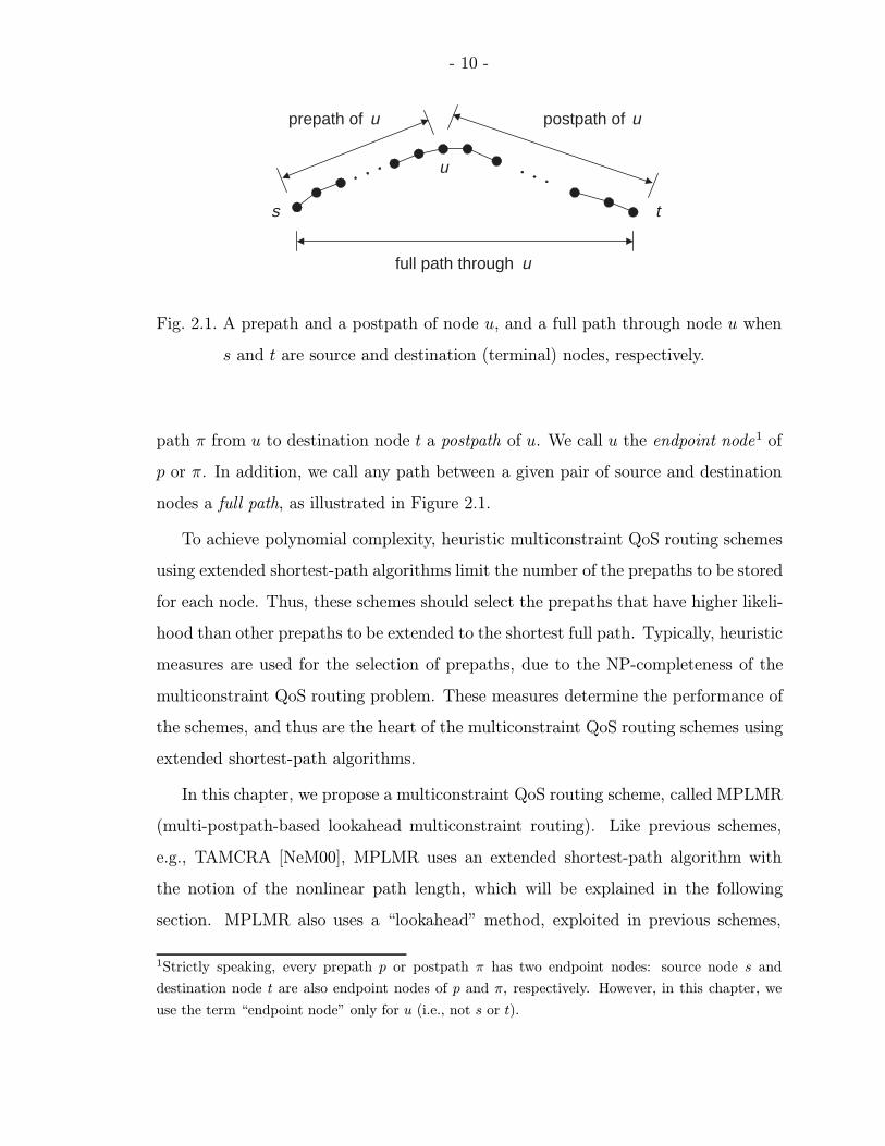
Before we describe our approach to solving the multiconstraint QoS routing prob-
lem, we introduce the following terms: prepath, postpath, and full path. For an
arbitrary node u, we call any path p from source node s to u a prepath of u, and any
- 10 -
u
s t
prepath of u postpath of u
full path through u
Fig. 2.1. A prepath and a postpath of node u, and a full path through node u when
s and t are source and destination (terminal) nodes, respectively.
path π from u to destination node t a postpath of u. We call u the endpoint node1 of
p or π. In addition, we call any path between a given pair of source and destination
nodes a full path, as illustrated in Figure 2.1.
To achieve polynomial complexity, heuristic multiconstraint QoS routing schemes
using extended shortest-path algorithms limit the number of the prepaths to be stored
for each node. Thus, these schemes should select the prepaths that have higher likeli-
hood than other prepaths to be extended to the shortest full path. Typically, heuristic
measures are used for the selection of prepaths, due to the NP-completeness of the
multiconstraint QoS routing problem. These measures determine the performance of
the schemes, and thus are the heart of the multiconstraint QoS routing schemes using
extended shortest-path algorithms.
In this chapter, we propose a multiconstraint QoS routing scheme, called MPLMR
(multi-postpath-based lookahead multiconstraint routing). Like previous schemes,
e.g., TAMCRA [NeM00], MPLMR uses an extended shortest-path algorithm with
the notion of the nonlinear path length, which will be explained in the following
section. MPLMR also uses a “lookahead” method, exploited in previous schemes,
1Strictly speaking, every prepath p or postpath π has two endpoint nodes: source node s and
destination node t are also endpoint nodes of p and π, respectively. However, in this chapter, we
use the term “endpoint node” only for u (i.e., not s or t).
- 11 -
e.g., H MCOP2 [KoK01]. That is, MPLMR considers postpaths associated with
prepaths for the selection of a limited number of prepaths to be stored during the
routing procedure. However, MPLMR uses a more effective lookahead method than
H MCOP. In contrast to H MCOP, which precomputes a single postpath for each
node, MPLMR precomputes multiple postpaths for each node. During the routing
procedure, MPLMR uses these postpaths to estimate the nonlinear path length of the
shortest full path to which each prepath is extended. Using this lookahead method,
MPLMR selects prepaths with higher likelihood than other prepaths to be extended
to the shortest full path. We show via simulation that MPLMR performs much better
than TAMCRA and H MCOP without sacrificing execution time.
The rest of this chapter is organized as follows. In Section 2.2, we introduce our
assumptions and notation, state the multiconstraint QoS routing problem, and discuss
the notions of nonlinear path length and lookahead methods. We summarize related
work on multiconstraint QoS routing in Section 2.3. In Section 2.4, we discuss the
approach of MPLMR to multiconstraint QoS routing. We describe the algorithm and
complexity of MPLMR in Section 2.5. In Section 2.6, we use simulation to evaluate
and compare MPLMR with competing schemes in the literature. We conclude in
Section 2.7.
2.2 Assumptions and definitions
2.2.1 Multiconstraint QoS routing problem
We assume that the following are given: a connected network topology, a source
node, a destination node, a set of QoS attribute values associated with each link, and
the QoS constraints that the routing path must satisfy. We assume that the net-
work topology is represented by an undirected graph, although we can treat network
2H MCOP searches for the path that not only is feasible but also minimizes the value of a primary
QoS attribute. However, if there is no primary QoS attribute designated, we can use H MCOP just
for finding a feasible path, as pointed out in [FeM02,KoK01,KuM02]. Throughout this chapter, we
assume that H MCOP does not have a primary QoS attribute designated.
- 12 -
topologies represented by directed graphs without additional difficulty. We also as-
sume that there is at most one link between any two nodes, that the network topology
does not change throughout the routing procedure, and that every QoS attribute is
additive, nonnegative, and fixed.
Because there is at most one link between any two nodes, we can represent any
link by its two endpoint nodes. We denote the link between arbitrary nodes u and v
by uv. To represent a path between two arbitrary nodes, we list all the nodes on the
path between ‘〈’ and ‘〉’. For example, we denote the path consisting of nodes u, v,
and w (in order) by 〈u, v, w〉. With this notation and all of the above assumptions,
we state the multiconstraint QoS routing problem as follows.
Definition 2.2.1 (Multiconstraint QoS Routing Problem) Suppose we are
given a connected graph representing a network topology, G = (V,E), where V
and E represent sets of n nodes and m links, respectively. Suppose also that
each link uv is characterized by nonnegative values with respect to q additive QoS
attributes, di(uv) ≥ 0, i = 1, . . . , q. Given a source node s, a destination node t,
and a constraint value Ci with respect to the ith QoS attribute for i = 1, . . . , q,
find a path p = 〈s, w1, . . . , wb, t〉, where wj, j = 1, . . . , b, is an intermediate node
on path p, such that the value of path p with respect to the ith QoS attribute, i.e.,
Li(p) = di(sw1) + di(w1w2) + . . .+ di(wbt), is less than or equal to the corresponding
constraint value Ci for every i = 1, . . . , q.
2.2.2 Nonlinear path length
One approach to solving the multiconstraint QoS routing problem is to use an
extended shortest-path algorithm. However, the “length” of a path in the multicon-
straint QoS routing problem cannot be defined as in the single-constraint shortest-
path problem. To resolve this difficulty, Neve and Mieghem [NeM00] propose the
notion of nonlinear path length, described as follows. Let Ci and Li(p) for i = 1, . . . , q
- 13 -
be as defined in Definition 2.2.1. Also define the normalized length of path p with
respect to the ith QoS attribute, denoted by NLi(p), as follows:
NLi(p) =Li(p)
Ci. (2.1)
The nonlinear path length of p, denoted by Λ(p), is defined to be the maximum of
the normalized lengths of p with respect to each QoS attribute, as follows:3
Λ(p) = max [NL1(p), NL2(p), . . . , NLq(p)] . (2.2)
It is straightforward to see that path p is feasible if and only if Λ(p) ≤ 1. For
the single-constraint QoS routing problem, this reduces to that p is feasible if and
only if LI(p)/C1 ≤ 1. Therefore, the nonlinear path length provides a basis for using
a standard (single-constraint) shortest-path algorithm for the multiconstraint QoS
routing problem. However, standard shortest-path algorithms rely on the property
that the length of a path is the sum of quantities associated only with individual
links on the path, a property that fails to hold for the nonlinear path length. For this
reason, multiconstraint QoS routing schemes using the nonlinear path length as the
measure for the “length” of a path entails a modification of the standard approach
(the modification will be described in the following sections).
2.2.3 Eligibility test and lookahead method
An arbitrary prepath p of a node u is dominated [Hen85] if there is another prepath
of u that has no larger value than p with respect to every QoS attribute, and has
strictly smaller values than p with respect to some QoS attributes. If p is dominated
by another prepath p′ of node u, and if p′ cannot be extended to a feasible path, then
p also cannot. Hence, a brute-force approach is to maintain a set for each node that
contains all nondominated prepaths found during the routing procedure, and extend
the prepaths to the destination node [WaV00]. When the algorithm terminates, we
3The definition here is a special case of the definition in [NeM00].
- 14 -
get all nondominated full paths, and thus we can check their feasibility. However,
this brute-force algorithm has exponential complexity.
To achieve polynomial complexity, extended shortest-path algorithms for multi-
constraint QoS routing limit the number of prepaths to be stored for each node.
Ideally, these schemes select prepaths that have higher likelihood than other prepaths
to be extended to the shortest full path (in terms of the modified “length,” the non-
linear path length). Eligibility tests and lookahead methods can be used for this
purpose.
Eligibility tests check if each prepath has the possibility to be extended to a feasible
path. We call a prepath eligible if it has any possibility to be extended to a feasible
path (eligibility depends on the specific test being used). By eliminating ineligible
prepaths from consideration, we can reduce the “search space” in which we search for
a feasible path.
The idea of lookahead methods is that the consideration of postpaths associated
with prepaths is helpful for selecting prepaths with higher likelihood than other
prepaths to be extended to the shortest full path. Using lookahead methods, we
estimate the nonlinear path length of the shortest full path to which each prepath is
extended. Due to the NP-completeness of the multiconstraint QoS routing problem,
we cannot consider all the postpaths associated with a given set of prepaths. Hence,
we first select some specific subset of the postpaths for applying a lookahead method,
as described later.
2.3 Related work
Neve and Mieghem propose a modification to the brute-force algorithm, called
TAMCRA [NeM00], by limiting the number of prepaths to be stored for each node.
TAMCRA includes an extended version of Dijkstra’s algorithm using the nonlinear
path length as the metric. During the course of the routing procedure, TAMCRA
stores for each node at most k shortest (in terms of nonlinear path length) prepaths
- 15 -
that have been found so far, hoping that these prepaths would have higher likelihood
than other prepaths to be extended to the shortest full path. However, TAMCRA
uses no lookahead method. That is, when TAMCRA selects the prepaths to be stored
for each node, the scheme considers the nonlinear path lengths of the prepaths only.
Hence, if an arbitrary node u finds a new prepath pn that has nonlinear path length
smaller than its kth shortest prepath pk, then pn replaces pk, even though prepath
pn may be connected to a much longer postpath than that of pk. Neve and Mieghem
also propose an alternative scheme, called SAMCRA [MiN01]. SAMCRA is almost
the same as TAMCRA, but SAMCRA does not limit the number of prepaths to be
stored for each node to guarantee finding an existing feasible path. Yuan proposes
a scheme called the limited path heuristic [Yua02], which is similar to TAMCRA.
However, for each node, the limited path heuristic stores the k prepaths that are not
necessarily the shortest. Yuan proves that low EDR can be achieved by maintaining
O(n2 log n) prepaths for each node, where n is the number of nodes.
To overcome the drawback of TAMCRA mentioned above, Korkmaz and Krunz
propose an enhanced scheme, called H MCOP [KoK01]. Different from TAMCRA,
H MCOP uses a lookahead method as follows. H MCOP precomputes a single post-
path for each node at the first step of the routing procedure, with the hope that
this single postpath would be the subpath of a feasible path through the node.
Then, H MCOP uses the postpath to update the set of at most k prepaths for each
node, with the goal that combining these prepaths with the postpath results in near-
minimum nonlinear path lengths. However, if the precomputed postpath is not the
subpath of a feasible path, then the postpath may misguide the selection of prepaths.
A* Prune [LiR01], proposed by Liu and Ramakrishnan for the problem of finding
multiple feasible paths, uses a lookahead method similar to the one in H MCOP. As
in SAMCRA, A* Prune does not limit the maximum number of prepaths to be stored
for each node.
There are several other approaches for solving the multiconstraint QoS routing
problem. Some multiconstraint QoS routing schemes partition the QoS attribute val-
- 16 -
ues into a finite number of intervals and apply dynamic programming techniques or
distributed routing techniques [Has92, Jaf84]. Some others prioritize QoS attributes
to search for the path that optimizes the value of the top-priority QoS attribute
under constraints on other QoS attributes [ChN99, ReS00, WaC96]. To reduce the
NP-complete multiconstraint QoS routing problem to one that is solvable in polyno-
mial time, some schemes approximate the given QoS attribute values [ChN98a,Yua02]
or network topologies via topology aggregation [ChH01]. Similarly, the dependencies
between QoS attributes are also exploited for the simplification of a given multi-
constraint QoS routing problem [MaS97, PoC97]. There are also schemes that pre-
compute the solutions to the expected routing problems to reduce the path-search
time [CuX03].
In our study, we do not compare our scheme with all of the above schemes, limiting
our comparison only to TAMCRA and H MCOP. The performance of the schemes in
[MiN01] and in [LiR01] corresponds to that of TAMCRA and H MCOP respectively,
when an infinite number of prepaths can be stored for each node to find a single
feasible path. Korkmaz and Krunz [KoK01] maintain that H MCOP is significantly
superior to the schemes in [ChN98a, Has92, Jaf84, Yua02]. The number of additive
QoS attributes to be considered in [ChN99,MaS97,PoC97,ReS00,WaC96] is limited
to only two or less. As topology aggregation is used in [ChH01], the imprecision
in estimating aggregated values of QoS attributes also accumulates, and this has a
significant negative impact on QoS routing [GuO97]. The precomputation scheme
in [CuX03] cannot solve routing problems if connection requests have QoS constraint
values for which solutions are not prepared in advanced.
2.4 Elements of our approach
2.4.1 Multiple postpaths
Our approach to multiconstraint QoS routing, called MPLMR (described in detail
in Section 2.5), uses an extended shortest-path routing algorithm based on the notion
- 17 -
sources
destinationt
u
at most k prepaths q postpaths
Fig. 2.2. Prepaths and postpaths for each node u.
of the nonlinear path length. Like previous schemes (e.g., TAMCRA and H MCOP),
MPLMR stores at most k prepaths for each node and updates them during the routing
procedure, with the intent that these prepaths have higher likelihood than other
prepaths to be extended to the shortest (in terms of nonlinear path length) full path.
In addition, MPLMR incorporates a lookahead method by selecting and storing q
postpaths for each node u at the beginning of the routing procedure (recall that q is
the number of QoS attributes), as is shown in Figure 2.2. Each of these postpaths is
the shortest path between u and destination node t with respect to the corresponding
QoS attribute, i.e., the ith postpath has the smallest value for the ith QoS attribute
among all possible postpaths. MPLMR uses these postpaths for the eligibility test
and the lookahead method, as described in the following sections.
2.4.2 Eligibility test of MPLMR
Let p be a prepath of an intermediate node u, πj(u) the shortest postpath of u
with respect to the jth QoS attribute for j = 1, . . . , q, and p + πj(u) the full path
combining p with πj(u). For each prepath p, MPLMR performs the following three
steps. (1) MPLMR checks if p is dominated by any other prepath stored for node u,
as TAMCRA does. If p is dominated by another prepath p′, MPLMR eliminates p
from consideration (because if p′ cannot be extended to a feasible path, then p also
cannot). (ii) If p is not dominated, MPLMR checks if the combined path p+ πj(u) is
- 18 -
feasible for j = 1, . . . , q. If any of these combined paths is feasible, then the routing
procedure terminates—this combined path solves the routing problem. (iii) If none of
the combined paths is feasible, MPLMR investigates the eligibility of p by checking if
NLj(p+ πj(u)) > 1 for any j = 1, . . . q, following the method introduced in [KoK99].
If NLj(p + πj(u)) > 1, then p is declared ineligible because every full path extended
from p violates the jth QoS constraint (recall that πj(u) is the shortest postpath of
u with respect to the jth QoS attribute)—in this case, MPLMR eliminates p from
consideration. Otherwise, p is declared eligible.
2.4.3 Lookahead method of MPLMR
Let node u, prepath p, and postpaths πj(u) be as given in Section 2.4.2. If the
combined path p + πj(u) is infeasible for j = 1, . . . , q, but if p is still eligible, then
MPLMR uses its lookahead method to estimate the nonlinear path length of the
shortest full path extended from p. To explain the lookahead method, let ps(p) be
the shortest (in terms of nonlinear path length) full path extended from p, and π∗
be the corresponding postpath of u (i.e., ps(p) = p + π∗). The basic idea in the
lookahead method of MPLMR is to estimate NLi(ps(p)) (i.e., the normalized length
of ps(p) with respect to the ith QoS attribute) as the weighted sum of NLi(p+πj(u))
(i.e., the normalized length of p + πj(u) with respect to the ith QoS attribute) for
j = 1, . . . , q. Let wij be the weight of NLi(p + πj(u)) used to estimate the value of
NLi(ps(p)). The estimated normalized length of ps(p) with respect to the ith QoS
attribute, denoted by NLi(ps(p)), is represented as follows:
NLi(ps(p)) =
q∑j=1
wijNLi(p+ πj(u)), (2.3)
where
q∑j=1
wij = 1. (2.4)
- 19 -
As in (2.2), the estimated nonlinear path length of ps(p), denoted by Λ(ps(p)), is
defined as follows:
Λ(ps(p)) = maxi=1,...,q
NLi(ps(p)). (2.5)
MPLMR uses Λ(ps(p)) as the basis to determine if p should be stored for node u.
As shown in (2.3) and (2.5), the estimated nonlinear path length of ps(p) is de-
termined by the estimated normalized lengths of ps(p), which depend on the weight
values wij for i = 1, . . . , q and j = 1, . . . , q. Hence, the selection of appropriate weight
values is important. To select the weight values, we take into account the following
two observations. First, ps(p) is likely to have a smaller normalized length with re-
spect to every QoS attribute than most of the full paths extended from p. Based on
this observation, our selection of the weights has the following property:
Property 1 For each i and j, the smaller the value of NLi(p+πj(u)), the larger the
value of wij in (2.3).
The second observation is the following. Because πj(u) is the shortest postpath
of node u with respect to the jth QoS attribute, NLj(ps(p)) ≥ NLj(p + πj(u)).
Thus, as the value of NLj(p+ πj(u)) becomes larger, it becomes more probable that
NLj(ps(p)) > 1, which is a violation of the jth QoS constraint. Hence, if the value
of NLj(p + πj(u)) is larger than the value of NLi(p + πi(u)) (recall that if p is an
eligible prepath, NLi(p+πi(u)) ≤ 1 is nonnegative for i = 1, . . . , q), then the jth QoS
constraint is more stringent than the ith QoS constraint. In this case, the satisfaction
of the jth QoS constraint must be given a higher priority than the ith QoS constraint
if we are to find a feasible path by extending prepath p toward the destination node.
For satisfying the jth QoS constraint, it is advantageous to take πj(u) as the postpath
to be connected to p. Hence, as the value of NLj(p + πj(u)) becomes larger, π∗ will
likely be “closer” to πj(u) (i.e., π∗ will likely share more links with πj(u)). Based on
this observation, our weight selection has the following property:
Property 2 For each j, the larger the value of NLj(p + πj(u)), the larger the value
of wij for all i in (2.3).
- 20 -
Let r be a nonnegative real constant. Based on Properties 1 and 2, MPLMR uses
the following weight wij for (2.3):
wij =ai
[NLi(p+ πj(u))]r[1−NLj(p+ πj(u))], (2.6)
where
ai =( q∑j=1
1
[NLi(p+ πj(u))]r[1−NLj(p+ πj(u))]
)−1
. (2.7)
In (2.6) and (2.7), ai is the value needed to satisfy the condition of (2.4) for i =
1, . . . , q, and r is a variable to control the relative contributions of NLi(p+πj(u)) and
1 − NLj(p + πj(u)) to wij. (The effect of r to the performance of MPLMR will be
described in Section 2.5.2.)
If NLi(p + πj(u)) = 0 or NLj(p + πj(u)) = 1, we cannot compute the value of
NLi(ps(p)) in (2.3) because the weight expression in (2.6) is not defined. To deal
with this difficulty, MPLMR sets NLi(ps(p)) = 0 if NLi(p + πj(u)) = 0, and simply
eliminates p from consideration if NLj(p + πj(u)) = 1 and u 6= t (recall that if
NLj(p+πj(u)) = 1 and u = t, then the routing procedure terminates because p+πj(u)
is a feasible path).
2.5 MPLMR: multi-postpath-based lookahead multiconstraint routing
2.5.1 MPLMR algorithm
The basic principle of MPLMR is to select and update at most k prepaths for
each node u during the routing procedure, as in previous schemes (e.g., TAMCRA and
H MCOP). However, in contrast to previous schemes, MPLMR selects the prepaths of
u to minimize the estimated nonlinear path lengths of the full paths containing these
prepaths (i.e., the values of (2.5).) To compute the estimated nonlinear path lengths
of (2.5), MPLMR uses (2.1), (2.3), (2.6), and (2.7). The pseudocode of MPLMR is
shown in Figure 2.3.
When a connection request occurs, MPLMR starts the routing procedure.
Lines 01–06 represent the initialization procedure of the modified Dijkstra’s algo-
- 21 -
MPLMR(G = (V,E), s, t, q, k, C1, . . . , Cq)
01 for every v ∈ V , do
02 find the shortest postpath πi(v) for i = 1, . . . , q /* using C1, . . . , Cq */
03 P (v)← {} /* P (v): set of prepaths to be stored for v */
04 if NLi(πi(s)) > 1 for any i = 1, . . . , q, then
05 stop /* routing failure: no feasible path */
06 Q← {〈s〉} /* Q: set of prepaths to be extended toward t */
07 while Q is not empty, do
08 x← a path in Q such that Λ(ps(x)) ≤ Λ(ps(p)) for any path p ∈ Q
09 w ← endpoint node of x
10 Q← Q− {x}
11 for each outgoing node u of w that is not on x, do
12 y ← x+ wu /* x extended to u */
13 if y is not dominated by another prepath of u in P (u), then
14 for each j = 1, . . . , q, do
15 if NLi(y + πj(u)) ≤ 1 for all i = 1, . . . , q, then
16 stop /* routing success: y + πj(u) is feasible */
17 if NLi(y + πi(u)) ≤ 1 for i = 1, . . . , q and |P (u)| < k, then
/* |P (u)|: number of paths in P (u) */
18 Q← Q ∪ {y} and P (u)← P (u) ∪ {y}
19 if NLi(y + πi(u)) ≤ 1 for i = 1, . . . , q and |P (u)| = k, then
20 z ← a path in P (u) such that Λ(ps(z)) ≥ Λ(ps(p)) for any p in P (u)
21 if Λ(ps(z)) > Λ(ps(y)), then
22 Q← Q ∪ {y} and P (u)← P (u)− {z} ∪ {y}
23 if z ∈ Q, then
24 Q← Q− {z}
25 stop /* routing failure: no feasible path found */
Fig. 2.3. The pseudocode of MPLMR.
- 22 -
rithm, described on lines 07–25. We can use any standard shortest-path algorithm
to find the q postpaths for every node on line 02. On lines 04–05, if the normalized
length of the ith postpath of source node s with respect to the ith QoS attribute
exceeds one, the routing procedure stops because no full path can satisfy the ith
QoS constraint. MPLMR maintains a set P (v) for each node v, and another set Q.
P (v) contains at most k prepaths of v, and Q contains prepaths (of any node) to be
extended toward t. On line 06, Q initially contains only a zero-length path from s to
itself.
While Q is not empty, MPLMR extracts from Q a prepath, denoted by x, such
that the estimated nonlinear path length of the shortest full path including x is the
smallest (lines 08–10). If the endpoint node of prepath x (denoted by w) has outgoing
nodes, then MPLMR extends x to an outgoing node u that is not on x (the extended
prepath is denoted by y on line 12). If y is not dominated by any other prepaths of
u that are stored in P (u), MPLMR performs the following tasks. (i) MPLMR checks
the feasibility of the full paths that consist of y and each of the postpaths of u. If
any of these full paths turns out to be feasible, then MPLMR outputs the path as
a solution to the multiconstraint QoS routing problem, and terminates the routing
procedure (lines 14–16). (ii) If none of the full paths is feasible, but if y is eligible
(i.e., NLi(y + πi(u)) ≤ 1 for i = 1, . . . , q), then MPLMR inserts y into Q and P (u).
However, in this case, if the number of the prepaths that are stored for u (in P (u))
exceeds k (by one), then MPLMR removes a prepath from Q and P (u), such that the
shortest full path extended from this prepath has a larger estimated nonlinear path
length than the shortest full paths extended from any other prepaths of u in P (u). If
there is no prepath in Q, then the routing procedure terminates on line 25 with no
feasible path found.
- 23 -
2.5.2 Control variable r
MPLMR uses the estimated nonlinear path length in (2.5) as the basis for selecting
the prepaths to be stored for each node. Because MPLMR computes the estimated
nonlinear path length using the weight values given in (2.6), the value of control
variable r of the weight affects the selection of prepaths. In (2.6), we can see that
the value of the weight becomes more dependent on Property 1 (Property 2) as the
value of r increases (decreases). Property 1 makes NLi(ps(p)) close to NLi(p+ πi(u))
for i = 1, . . . , q, which is the minimum value that NLi(ps(p)) could take from the
viewpoint of the endpoint node of p. Hence, the following proposition holds:
Proposition 2.5.1 Let p be a prepath of node u, ps(p) the shortest (in terms of
nonlinear path length) full path extended from p, and πj(u) the shortest postpath of
u with respect to the jth QoS attribute for j = 1, . . . , q. If NLi(p + πj(u)) 6= 0
and NLj(p + πj(u)) 6= 1 for i = 1, . . . , q and j = 1, . . . , q, then, limr→∞ Λ(ps(p)) ≤
Λ(ps(p)).
Proof Because πi(u) is the shortest postpath of u with respect to the ith QoS
attribute, NLi(p + πi(u)) ≤ NLi(p + πj(u)). If NLi(p + πi(u)) < NLi(p + πj(u)),
then wij → 0 as r → ∞ (see (2.6) and (2.7)). Hence, if wij 9 0 as r → ∞, then
NLi(p + πi(u)) = NLi(p + πj(u)). Thus, NLi(ps(p))→ NLi(p + πi(u)) as r →∞ for
i = 1, . . . , q by (2.3) and (2.4). Because of the same reason (i.e., πi(u) is the shortest
postpath of u with respect to the ith QoS attribute), NLi(p + πi(u)) ≤ NLi(ps(p))
for i = 1, . . . , q. Hence, NLi(ps(p)) ≤ NLi(ps(p)) for i = 1, . . . , q, and therefore
Λ(ps(p)) ≤ Λ(ps(p)) by (2.2) and (2.5).
In contrast, Property 2 makes NLi(ps(p)) close to NLi(p+πj(u)) for i = 1, . . . , q if
the jth QoS constraint is the most stringent for finding a feasible path by extending
prepath p toward the destination node. Thus, in this case, Λ(ps(p)) becomes closer to
Λ(p+ πj(u)) as the value of r decreases. Note that Λ(p+ πj(u)) must be larger than
or equal to Λ(ps(p)), and that Λ(ps(p)) does not necessarily converge to Λ(p+ πj(u))
as r→ 0.
- 24 -
uprepath p
postpathπ1(u)
postpathπ2(u)
NL1(p + π1(u))= 0.5
NL2(p + π1(u))= 1.1
NL1(p + π2(u))= 2.0
NL2(p + π2(u))= 0.9
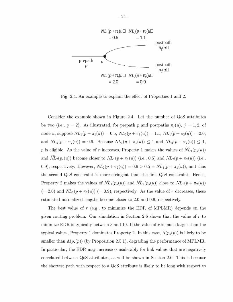
Fig. 2.4. An example to explain the effect of Properties 1 and 2.
Consider the example shown in Figure 2.4. Let the number of QoS attributes
be two (i.e., q = 2). As illustrated, for prepath p and postpaths πj(u), j = 1, 2, of
node u, suppose NL1(p + π1(u)) = 0.5, NL2(p + π1(u)) = 1.1, NL1(p + π2(u)) = 2.0,
and NL2(p + π2(u)) = 0.9. Because NL1(p + π1(u)) ≤ 1 and NL2(p + π2(u)) ≤ 1,
p is eligible. As the value of r increases, Property 1 makes the values of NL1(ps(u))
and NL2(ps(u)) become closer to NL1(p+ π1(u)) (i.e., 0.5) and NL2(p + π2(u)) (i.e.,
0.9), respectively. However, NL2(p + π2(u)) = 0.9 > 0.5 = NL1(p + π1(u)), and thus
the second QoS constraint is more stringent than the first QoS constraint. Hence,
Property 2 makes the values of NL1(ps(u)) and NL2(ps(u)) close to NL1(p + π2(u))
(= 2.0) and NL2(p + π2(u)) (= 0.9), respectively. As the value of r decreases, these
estimated normalized lengths become closer to 2.0 and 0.9, respectively.
The best value of r (e.g., to minimize the EDR of MPLMR) depends on the
given routing problem. Our simulation in Section 2.6 shows that the value of r to
minimize EDR is typically between 3 and 10. If the value of r is much larger than the
typical values, Property 1 dominates Property 2. In this case, Λ(ps(p)) is likely to be
smaller than Λ(ps(p)) (by Proposition 2.5.1), degrading the performance of MPLMR.
In particular, the EDR may increase considerably for link values that are negatively
correlated between QoS attributes, as will be shown in Section 2.6. This is because
the shortest path with respect to a QoS attribute is likely to be long with respect to
- 25 -
s t
v1
(0, 3)
Cd = Cc = 10
v2
v3
u
v5
v4
(4, 2)
(4, 0)
(2, 5)
(4, 3)
(5, 0)
(0, 4)
(2, 3)
(0, 5)
(2, 1)
p1 = <s, v1, u >
p2 = <s, v2, u>
p3 = <s, v3, u >
p4 = <u, v4, t >
p5 = <u, v5, t >
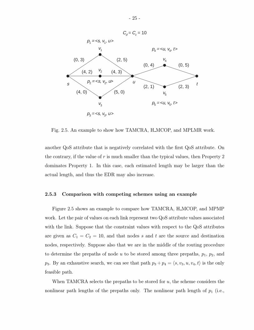
Fig. 2.5. An example to show how TAMCRA, H MCOP, and MPLMR work.
another QoS attribute that is negatively correlated with the first QoS attribute. On
the contrary, if the value of r is much smaller than the typical values, then Property 2
dominates Property 1. In this case, each estimated length may be larger than the
actual length, and thus the EDR may also increase.
2.5.3 Comparison with competing schemes using an example
Figure 2.5 shows an example to compare how TAMCRA, H MCOP, and MPMP
work. Let the pair of values on each link represent two QoS attribute values associated
with the link. Suppose that the constraint values with respect to the QoS attributes
are given as C1 = C2 = 10, and that nodes s and t are the source and destination
nodes, respectively. Suppose also that we are in the middle of the routing procedure
to determine the prepaths of node u to be stored among three prepaths, p1, p2, and
p3. By an exhaustive search, we can see that path p3 + p4 = 〈s, v3, u, v4, t〉 is the only
feasible path.
When TAMCRA selects the prepaths to be stored for u, the scheme considers the
nonlinear path lengths of the prepaths only. The nonlinear path length of p1 (i.e.,
- 26 -
Λ(p1)) is 0.8 (i.e., min [(0 + 2)/10, (3 + 5)/10]). Similarly, Λ(p2) and Λ(p3) are 0.8
and 0.9, respectively. Because Λ(p3) > Λ(p1) = Λ(p2), TAMCRA selects p3 to store
for u only if the maximum number of prepaths to be stored for each node (i.e., k) is
at least three. Thus, TAMCRA finds a feasible path only if k ≥ 3.
Recall that H MCOP selects a single postpath for each node. Among all possible
postpaths for each node, the selected postpath should have the minimum value of the
sum of normalized lengths. Hence, H MCOP selects path p5 as this single postpath
of node u, because the corresponding value for path p5 (i.e., NL1(p5)+NL2(p5) = 0.8)
is smaller than that for path p4 (i.e., NL1(p4) + NL2(p4) = 0.9). When path p5 is
connected with the prepaths of u, p1 + p5, p2 + p5, and p3 + p5 have nonlinear path
lengths of 1.2, 1.2, and 1.3, respectively. Because Λ(p3+p5) > Λ(p1+p5) = Λ(p2+p5),
H MCOP stores p3 for u only if k ≥ 3. Thus, H MCOP also finds a feasible path only
if k ≥ 3.
p4 and p5 are the shortest paths between u and t with respect to the first and
the second QoS attributes, respectively. Hence, MPLMR selects paths p4 and p5
as the postpaths of node u with respect to the first and the second QoS attributes,
respectively (i.e., π1(u) = p4 and π2(u) = p5). Suppose that r = 5. Using (2.1),
MPLMR computes the normalized lengths of all the full paths in Figure 2.5, as shown
in Table 2.1. Because NL2(p1 + π2(u)) = 1.2 > 1.0, p1 is ineligible. Hence, MPLMR
eliminates p1 from consideration. Using (2.6), (2.7), and the values in Table 2.1,
MPLMR also computes the weight values in Table 2.2. From (2.3) and the values
in Tables 2.1 and 2.2, NL1(ps(p2)) = w11NL1(p2 + π1(u)) + w12NL1(p2 + π2(u)) =
0.884. Similarly, NL2(ps(p2)) = 0.926, NL1(ps(p3)) = 0.910, and NL2(ps(p3)) = 0.447.
Hence, the estimated nonlinear path lengths of the shortest full paths extended from
p2 and p3 (i.e., Λ(ps(p2)) and Λ(ps(p3))) are 0.926 and 0.910, respectively. Because
Λ(ps(p3)) < Λ(ps(p2)), MPLMR selects p3 first. Therefore, MPLMR finds a feasible
path even for k = 1.

- 27 -
Table 2.1
The normalized lengths of all the full paths in Figure 2.5.
NL1(p1 + π1(u)) = 0.2 NL2(p1 + π1(u)) = 1.7
NL1(p1 + π2(u)) = 0.6 NL2(p1 + π2(u)) = 1.2
NL1(p2 + π1(u)) = 0.8 NL2(p2 + π1(u)) = 1.4
NL1(p2 + π2(u)) = 1.2 NL2(p2 + π2(u)) = 0.9
NL1(p3 + π1(u)) = 0.9 NL2(p3 + π1(u)) = 0.9
NL1(p3 + π2(u)) = 1.3 NL2(p3 + π2(u)) = 0.4
Table 2.2
The values used to compute the estimated nonlinear path lengths of the shortest full
paths extended from p2 and p3.
For p2,
w11 = 0.792, w12 = 0.208, w21 = 0.052, and w22 = 0.948.
(a1 = 0.0519 and a2 = 0.0560)
For p3,
w11 = 0.974, w12 = 0.026, w21 = 0.094, and w22 = 0.906.
(a1 = 0.0575 and a2 = 0.0056).
- 28 -
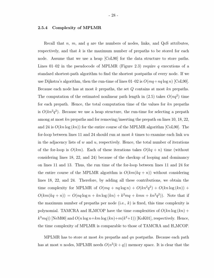
2.5.4 Complexity of MPLMR
Recall that n, m, and q are the numbers of nodes, links, and QoS attributes,
respectively, and that k is the maximum number of prepaths to be stored for each
node. Assume that we use a heap [CoL90] for the data structure to store paths.
Lines 01–02 in the pseudocode of MPLMR (Figure 2.3) require q executions of a
standard shortest-path algorithm to find the shortest postpaths of every node. If we
use Dijkstra’s algorithm, then the run-time of lines 01–02 is O(mq+nq logn) [CoL90].
Because each node has at most k prepaths, the set Q contains at most kn prepaths.
The computation of the estimated nonlinear path length in (2.5) takes O(nq2) time
for each prepath. Hence, the total computation time of the values for kn prepaths
is O(kn2q2). Because we use a heap structure, the run-time for selecting a prepath
among at most kn prepaths and for removing/inserting the prepath on lines 10, 18, 22,
and 24 is O(kn log (kn)) for the entire course of the MPLMR algorithm [CoL90]. The
for-loop between lines 11 and 24 should run at most k times to examine each link wu
in the adjacency lists of w and u, respectively. Hence, the total number of iterations
of the for-loop is O(km). Each of these iterations takes O(kq + n) time (without
considering lines 18, 22, and 24) because of the checkup of looping and dominancy
on lines 11 and 13. Thus, the run time of the for-loop between lines 11 and 24 for
the entire course of the MPLMR algorithm is O(km(kq + n)) without considering
lines 18, 22, and 24. Therefore, by adding all these contributions, we obtain the
time complexity for MPLMR of O(mq + nq logn) + O(kn2q2) + O(kn log (kn)) +
O(km(kq + n)) = O(nq log n + kn log (kn) + k2mq + kmn + kn2q2)). Note that if
the maximum number of prepaths per node (i.e., k) is fixed, this time complexity is
polynomial. TAMCRA and H MCOP have the time complexities of O(kn log (kn) +
k3mq)) [NeM00] andO(n logn+km log (kn)+m(k2+1)) [KoK01], respectively. Hence,
the time complexity of MPLMR is comparable to those of TAMCRA and H MCOP.
MPLMR has to store at most kn prepaths and qn postpaths. Because each path
has at most n nodes, MPLMR needs O(n2(k+ q)) memory space. It is clear that the
- 29 -
EDR of MPLMR decreases as the value of k increases. Hence, MPLMR achieves low
EDR at the expense of the increased run time and the memory space for an increased
number of prepaths.
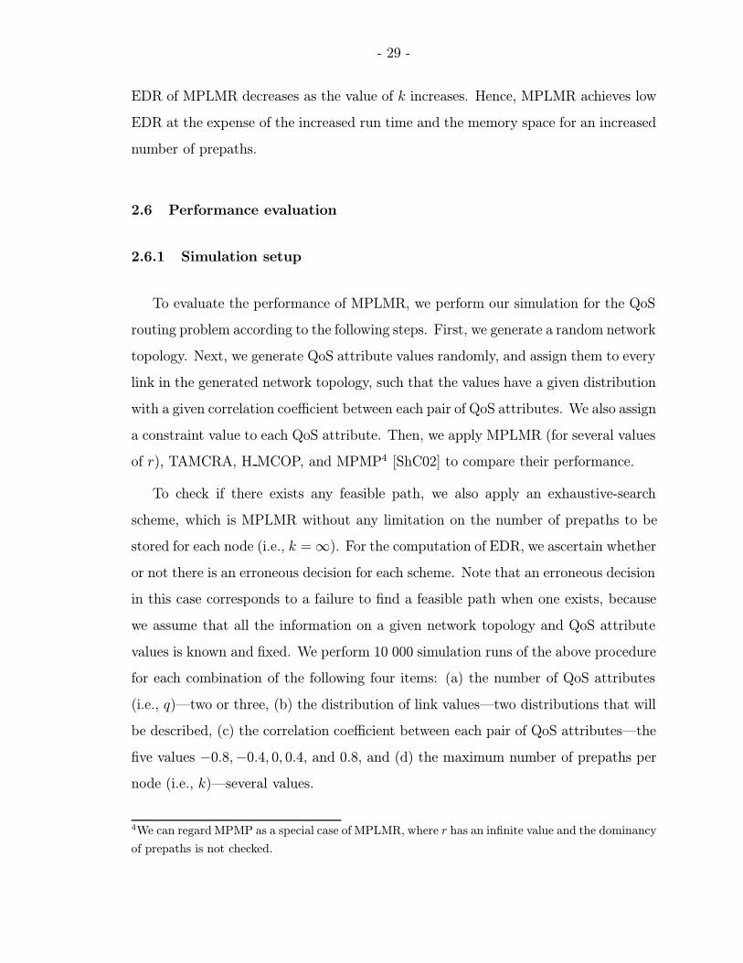
2.6 Performance evaluation
2.6.1 Simulation setup
To evaluate the performance of MPLMR, we perform our simulation for the QoS
routing problem according to the following steps. First, we generate a random network
topology. Next, we generate QoS attribute values randomly, and assign them to every
link in the generated network topology, such that the values have a given distribution
with a given correlation coefficient between each pair of QoS attributes. We also assign
a constraint value to each QoS attribute. Then, we apply MPLMR (for several values
of r), TAMCRA, H MCOP, and MPMP4 [ShC02] to compare their performance.
To check if there exists any feasible path, we also apply an exhaustive-search
scheme, which is MPLMR without any limitation on the number of prepaths to be
stored for each node (i.e., k =∞). For the computation of EDR, we ascertain whether
or not there is an erroneous decision for each scheme. Note that an erroneous decision
in this case corresponds to a failure to find a feasible path when one exists, because
we assume that all the information on a given network topology and QoS attribute
values is known and fixed. We perform 10 000 simulation runs of the above procedure
for each combination of the following four items: (a) the number of QoS attributes
(i.e., q)—two or three, (b) the distribution of link values—two distributions that will
be described, (c) the correlation coefficient between each pair of QoS attributes—the
five values −0.8,−0.4, 0, 0.4, and 0.8, and (d) the maximum number of prepaths per
node (i.e., k)—several values.
4We can regard MPMP as a special case of MPLMR, where r has an infinite value and the dominancy
of prepaths is not checked.
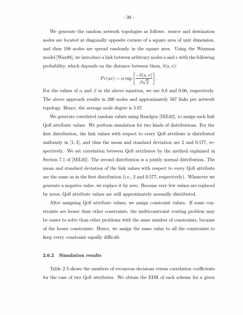
- 30 -
We generate the random network topologies as follows: source and destination
nodes are located at diagonally opposite corners of a square area of unit dimension,
and then 198 nodes are spread randomly in the square area. Using the Waxman
model [Wax88], we introduce a link between arbitrary nodes u and v with the following
probability, which depends on the distance between them, δ(u, v):
Pr(uv) = α exp
[−δ(u, v)
β√
2
].
For the values of α and β in the above equation, we use 0.8 and 0.06, respectively.
The above approach results in 200 nodes and approximately 567 links per network
topology. Hence, the average node degree is 5.67.
We generate correlated random values using Randgen [MiL02], to assign each link
QoS attribute values. We perform simulation for two kinds of distributions. For the
first distribution, the link values with respect to every QoS attribute is distributed
uniformly in [1, 3], and thus the mean and standard deviation are 2 and 0.577, re-
spectively. We set correlation between QoS attributes by the method explained in
Section 7.1 of [MiL02]. The second distribution is a jointly normal distribution. The
mean and standard deviation of the link values with respect to every QoS attribute
are the same as in the first distribution (i.e., 2 and 0.577, respectively). Whenever we
generate a negative value, we replace it by zero. Because very few values are replaced
by zeros, QoS attribute values are still approximately normally distributed.
After assigning QoS attribute values, we assign constraint values. If some con-
straints are looser than other constraints, the multiconstraint routing problem may
be easier to solve than other problems with the same number of constraints, because
of the looser constraints. Hence, we assign the same value to all the constraints to
keep every constraint equally difficult.
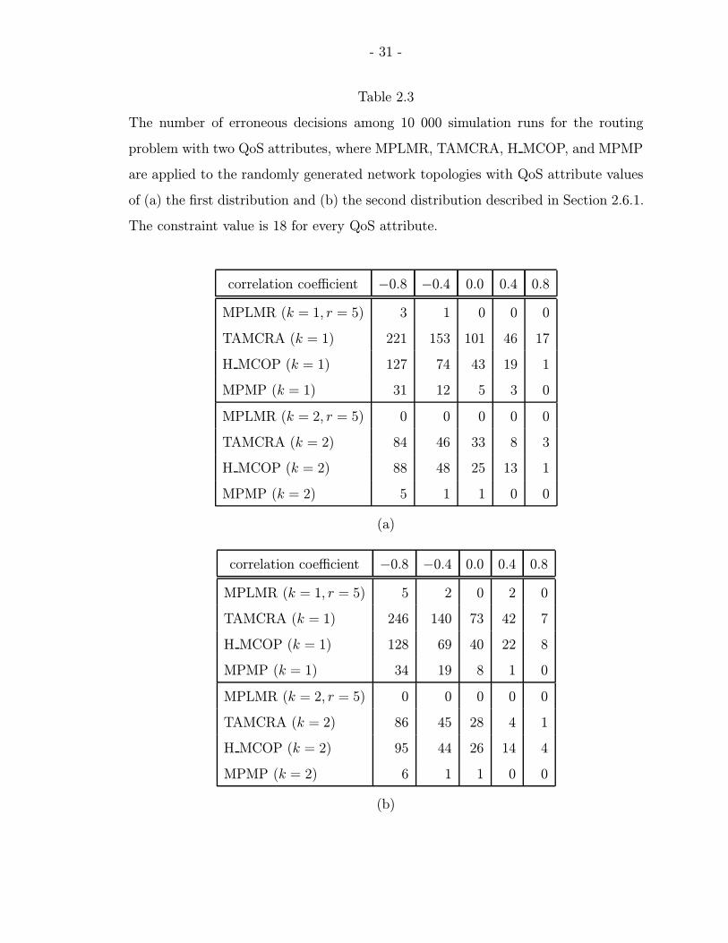
2.6.2 Simulation results
Table 2.3 shows the numbers of erroneous decisions versus correlation coefficients
for the case of two QoS attributes. We obtain the EDR of each scheme for a given
- 31 -
Table 2.3
The number of erroneous decisions among 10 000 simulation runs for the routing
problem with two QoS attributes, where MPLMR, TAMCRA, H MCOP, and MPMP
are applied to the randomly generated network topologies with QoS attribute values
of (a) the first distribution and (b) the second distribution described in Section 2.6.1.
The constraint value is 18 for every QoS attribute.
correlation coefficient −0.8 −0.4 0.0 0.4 0.8
MPLMR (k = 1, r = 5) 3 1 0 0 0
TAMCRA (k = 1) 221 153 101 46 17
H MCOP (k = 1) 127 74 43 19 1
MPMP (k = 1) 31 12 5 3 0
MPLMR (k = 2, r = 5) 0 0 0 0 0
TAMCRA (k = 2) 84 46 33 8 3
H MCOP (k = 2) 88 48 25 13 1
MPMP (k = 2) 5 1 1 0 0
(a)
correlation coefficient −0.8 −0.4 0.0 0.4 0.8
MPLMR (k = 1, r = 5) 5 2 0 2 0
TAMCRA (k = 1) 246 140 73 42 7
H MCOP (k = 1) 128 69 40 22 8
MPMP (k = 1) 34 19 8 1 0
MPLMR (k = 2, r = 5) 0 0 0 0 0
TAMCRA (k = 2) 86 45 28 4 1
H MCOP (k = 2) 95 44 26 14 4
MPMP (k = 2) 6 1 1 0 0
(b)
- 32 -
correlation coefficient by dividing the number of erroneous decisions by the number
of simulation runs (i.e., 10 000). We can see that MPLMR has lower EDR than
TAMCRA, H MCOP, and MPMP, for all the correlation coefficients. This observation
applies to both the distributions in (a) and (b). Table 2.4 shows simulation results
for the case of three QoS attributes: the first two are the same as in Table 2.3, and
the third QoS attribute is uncorrelated with each of the first two. Again we observe
that MPLMR has lower EDR than the other schemes. We show results in Table 2.4
only for the first distribution, because the results for the second distribution are very
similar.
For the above simulation, the used constraint value is 18 (recall that the same
constraint value is used for every QoS attribute). As shown in Figure 2.6, the value of
the most stringent constraint is close to 18. Hence, the EDR computed from Tables 2.3
and 2.4 is the value for a near-worst case. If the constraint value is smaller than
18, then the EDR decreases because the number of the instances without solutions
increases. That is, the probability of missing a feasible path decreases because there
is no feasible path in many simulation runs. If the constraint value is larger than 18,
the EDR decreases because the constraints are loose.
In our simulation, the execution time of MPLMR is approximately 80% of the
execution time of MPMP, and just 30-40% of the execution time of TAMCRA and
H MCOP. Recall that the asymptotic time complexity of MPLMR is comparable to
those of TAMCRA, H MCOP, and MPMP. However, MPLMR has a shorter execution
time compared to the other schemes because of the following two reasons. First, in
contrast to TAMCRA and MPMP, MPLMR stores multiple postpaths (not just the
values of postpaths). Hence, if the full path consisting of a prepath and a postpath
is feasible, MPLMR terminates the routing without extending the prepath toward
the destination node. Next, in contrast to H MCOP, MPLMR performs an eligibility
test to discard ineligible prepaths. Thus, MPLMR reduces the search space where
the scheme searches for a feasible path.
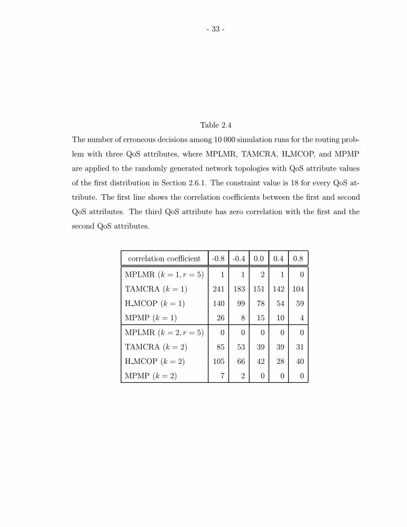
- 33 -
Table 2.4
The number of erroneous decisions among 10 000 simulation runs for the routing prob-
lem with three QoS attributes, where MPLMR, TAMCRA, H MCOP, and MPMP
are applied to the randomly generated network topologies with QoS attribute values
of the first distribution in Section 2.6.1. The constraint value is 18 for every QoS at-
tribute. The first line shows the correlation coefficients between the first and second
QoS attributes. The third QoS attribute has zero correlation with the first and the
second QoS attributes.
correlation coefficient -0.8 -0.4 0.0 0.4 0.8
MPLMR (k = 1, r = 5) 1 1 2 1 0
TAMCRA (k = 1) 241 183 151 142 104
H MCOP (k = 1) 140 99 78 54 59
MPMP (k = 1) 26 8 15 10 4
MPLMR (k = 2, r = 5) 0 0 0 0 0
TAMCRA (k = 2) 85 53 39 39 31
H MCOP (k = 2) 105 66 42 28 40
MPMP (k = 2) 7 2 0 0 0
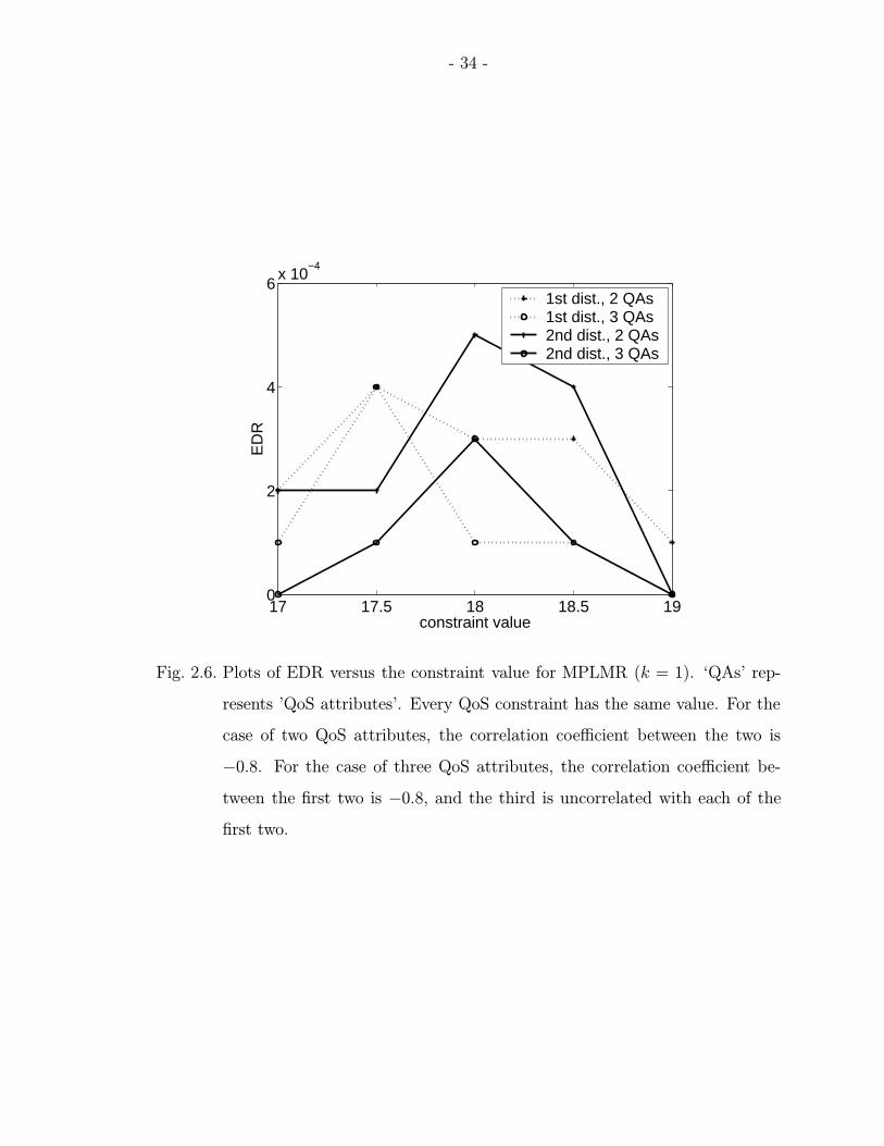
- 34 -
17 17.5 18 18.5 190
2
4
6x 10
−4
constraint value
ED
R
1st dist., 2 QAs1st dist., 3 QAs2nd dist., 2 QAs2nd dist., 3 QAs
Fig. 2.6. Plots of EDR versus the constraint value for MPLMR (k = 1). ‘QAs’ rep-
resents ’QoS attributes’. Every QoS constraint has the same value. For the
case of two QoS attributes, the correlation coefficient between the two is
−0.8. For the case of three QoS attributes, the correlation coefficient be-
tween the first two is −0.8, and the third is uncorrelated with each of the
first two.
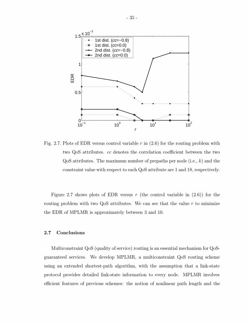
- 35 -
10−1
100
101
102
0
0.5
1
1.5x 10
−3
r
ED
R
1st dist. (cc=−0.8)1st dist. (cc=0.0) 2nd dist. (cc=−0.8)2nd dist. (cc=0.0)
Fig. 2.7. Plots of EDR versus control variable r in (2.6) for the routing problem with
two QoS attributes. cc denotes the correlation coefficient between the two
QoS attributes. The maximum number of prepaths per node (i.e., k) and the
constraint value with respect to each QoS attribute are 1 and 18, respectively.
Figure 2.7 shows plots of EDR versus r (the control variable in (2.6)) for the
routing problem with two QoS attributes. We can see that the value r to minimize
the EDR of MPLMR is approximately between 3 and 10.
2.7 Conclusions
Multiconstraint QoS (quality of service) routing is an essential mechanism for QoS-
guaranteed services. We develop MPLMR, a multiconstraint QoS routing scheme
using an extended shortest-path algorithm, with the assumption that a link-state
protocol provides detailed link-state information to every node. MPLMR involves
efficient features of previous schemes: the notion of nonlinear path length and the
- 36 -
dominancy check as in TAMCRA [NeM00], the eligibility test as in the randomized al-
gorithm of [KoK99], and a lookahead feature as in H MCOP [KoK01]. MPLMR uses
not only these existing features but also an improved lookahead method. Using this
lookahead method, MPLMR estimates the nonlinear path length of the shortest (in
terms of nonlinear path length) full path to which each prepath is extended. Based on
the estimated nonlinear path lengths, MPLMR selects and stores a limited number of
prepaths that have higher likelihood than other prepaths to be extended to the short-
est full path. The asymptotic worst-case complexity of MPLMR is comparable with
those of TAMCRA and H MCOP. However, we show via simulation that MPLMR
achieves much lower EDR than the schemes. Furthermore, MPLMR achieves the low
EDR with even smaller execution time than the competing schemes. Hence, MPLMR
provides a promising solution for multiconstraint QoS routing, which will become an
essential tool for high-quality communication/computer services in the near future.
- 37 -
3. DISTRIBUTED MULTICONSTRAINT QOS ROUTING
USING A DEPTH-FIRST SEARCH METHOD BASED ON
DISTANCE-VECTOR PROTOCOLS
3.1 Introduction
In this chapter, we deal with the same routing problem as in the previous chapter
(i.e., the multiconstraint QoS routing problem). However, our goal in this chapter is
to develop an efficient multiconstraint QoS routing scheme for routing environments
where signaling overhead must be minimized (e.g., wireless ad-hoc networks where
power and bandwidth are limited). Hence, we have different assumptions on infor-
mation advertisement, which significantly affects the signaling overhead for routing.
We have three choices for information advertisement in multiconstraint QoS rout-
ing: (a) no advertisement of routing information, (b) the use of a link-state protocol,
and (c) the use of a distance-vector protocol. If routing information is not adver-
tised, “flooding” must be used for path search when a connection request occurs at a
(source) node. That is, the source node forwards the connection request message to
all the neighboring nodes, and every node that receives the message forwards it again
to all its neighboring nodes. This forward of connection request messages terminates
when some stopping condition is met. Hence, flooding-based path search usually
causes a significant amount of signaling overhead during the path-search period, and
is highly likely to involve many unnecessary nodes in the path-search process. In
contrast, the use of a link-state protocol for information advertisement may cause
heavy signaling overhead in the information-advertisement process because detailed
routing information of each link is distributed to every node in a given network.
To avoid heavy signaling overhead in both the information-advertisement and path-
search processes, we assume that a distance-vector protocol is used for information
- 38 -
advertisement (recall that the use of a link-state protocol is assumed in the previous
chapter).
If we use a distance-vector protocol for information advertisement, each node u
has only the following information with respect to each of the attributes considered:
(a) the estimated value of the best path between u and every other node, and (b)
the next-hop node on the path. Thus, in multiconstraint QoS routing, the source
node that receives a connection request cannot find a feasible path for the connection
request, without the help of other nodes. Hence, distributed routing schemes must be
used. Distributed routing schemes forward the connection request message from the
source node toward the destination node. Whenever the connection request message is
forwarded, the path along which the connection request message has passed is updated
and recorded in the connection request message. Henceforth, we refer to this prepath
as the history path of the connection request message. During the routing procedure,
each connection request message whose history path is ineligible (i.e., not able to
be extended into a feasible path) is discarded or sent back to the predecessor node.
If any connection request message arrives the destination node without violating
constraints, then the routing process reserves the network resources of the history
path of the connection request message, and terminates.
To reduce the signaling overhead in the distributed path search, the connection
request message should be forwarded “selectively”. That is, if an arbitrary node
receives a connection request message, this node should forward it only to its neigh-
boring nodes that are highly probable to be on feasible paths. For the selection of such
neighboring nodes, we first develop a metric, called the minimum normalized margin
(NMmin), which measures the severity of the strictest constraint. The NMmin is com-
puted from the routing information provided by distance-vector protocols. We then
develop an efficient distributed multiconstraint QoS routing scheme, called SPMP
(single-prepath multi-postpaths), which uses the NMmin.
As described in the previous chapter, there are many approaches for solving the
multiconstraint QoS routing problem. However, a sequential path-search approach
- 39 -
has not been developed in the literature beyond simple depth-first search. Asymptotic
exponential worst-case time complexity is the critical drawback of the sequential path-
search approach. However, SPMP takes a sequential search approach using a depth-
first search method that controls the worst-case time complexity. At any time during
the path-search procedure, SPMP maintains only a single prepath, and attempts to
extend it to a feasible path. By taking this sequential approach, SPMP minimizes
the number of the nodes involved in path search at the expense of possible increase
in the path-search time. Moreover, for the reduction of the path-search time, SPMP
takes a multiple-postpath approach similar to that of MPLMR.
The rest of this chapter is organized as follows. In Section 3.2, we introduce
our assumptions and notation. We define the NMmin in Section 3.3.1, and describe
SPMP in detail in 3.4. In Section 3.5, we use simulation to evaluate the performance
of SPMP. We conclude in Section 3.6.
3.2 Assumptions and definitions
For the routing information that a connection request contains, we make the
same assumptions as in the previous chapter. Hence, we assume that the following
are given: a network topology (which is represented by an undirected graph), a source
node, a destination node, and the constraint that the routing path must satisfy with
respect to each QoS attribute. We also assume that there is at most one link between
any two nodes, that the network topology does not change throughout the routing
procedure, and that every QoS attribute is nonnegative and fixed. However, in this
chapter, we assume that a distance-vector protocol provides each node u with the
following routing information for every pair of a node v and a QoS attribute: the
value of the best path between u and v with respect to the QoS attribute, and the
next-hop node on the best path (recall that we assume the use of a link-state protocol
for information advertisement in the previous chapter).
- 40 -
Every QoS attribute is either a min/max attribute or a cumulative attribute (i.e.,
an additive attribute and a multiplicative attribute). In this chapter, we consider
only additive attributes to develop our routing scheme, as in the previous chap-
ter. However, with some minor changes, this scheme can be easily extended for the
routing problems that have constraints on min/max attributes as well. Recall that
multiplicative attributes can be regarded as additive by taking logarithm. Because
of the additivity of QoS attributes considered, we can still regard the value of a path
with respect to a QoS attribute as the “length” of the path with respect to the QoS
attribute.
Other than the use of a distance-vector protocol (instead of a link-state protocol),
we have the same assumptions in this chapter as in the previous chapter. Hence, we
deal with the same multiconstraint QoS routing problem. This problem is restated
as follows:
Definition 3.2.1 (Restatement of Multiconstraint QoS Routing Problem)
Suppose we are given a connected graph representing a network topology, G = (V,E),
where V and E represent sets of n nodes and m links, respectively. Suppose also
that each link uv is characterized by nonnegative values with respect to q additive
QoS attributes, di(uv) ≥ 0, i = 1, . . . , q. Given a source node s, a destination node
t, and a constraint value Ci with respect to the ith QoS attribute for i = 1, . . . , q,
find a path p = 〈s, w1, . . . , wb, t〉, where wj, j = 1, . . . , b, is an intermediate node
on path p, such that the value of p with respect to the ith QoS attribute, i.e.,
Li(p) = di(sw1) + di(w1w2) + . . .+ di(wbt), is less than or equal to the corresponding
constraint value Ci for every i = 1, . . . , q.
3.3 Elements of our approach
3.3.1 Minimum normalized margin
For arbitrary nodes u and v in a given network, let A(u, v) be the set of all
possible paths between u and v, a an arbitrary path in A(u, v), b(a) the number of
- 41 -
links on path a, wa,i the ith node along a, and wa,i−1wa,i the link between wa,i−1 and
wa,i. In the previous section, we assumed that a distance-vector protocol provides u
the following value, denoted by Rj(u, v), with respect to the jth QoS attribute for
j = 1, . . . , q and for every node v in the network.
Rj(u, v) = mina∈A(u,v)
b(a)∑i=1
dj(wa,i−1wa,i),
where wa,0 = u and wa,b(a) = v.
Suppose that a connection request message arrives at u, with the following infor-
mation: the history path p from s to u, destination node t, and constraint value Cj
with respect to the jth QoS attribute for j = 1, . . . , q. Note that p is a prepath of
u. Based on the value of Rj(u, t) and Cj, node u can compute the following value,
denoted by NRj(u):
NRj(u) =Rj(u, t)
Cj.
Henceforth, we call NRj(u) the normalized requirement of node u for the jth QoS
attribute. Note that NRj(u) is the minimum path length with respect to the jth
QoS attribute (as a fraction of Cj) of any postpath of node u. Because QoS attribute
values of every link are nonnegative, NRj(u) ≥ 0.
Recall that Lj(p) and NLj(p) be the length and the normalized length respectively,
of path p with respect to the jth QoS attribute (see Section 2.2.2). The normalized
margin of p with respect to the jth QoS attribute, denoted by NMj(p), is defined as
follows:
NMj(p) = 1−[NLj(p) +NRj(u)
]=
1
Cj· maxa∈A(u,t)
[Cj − Lj(p)− Lj(a)
]Hence, NMj(p) corresponds to the upper bound of the difference between the jth
constraint value (i.e., Cj) and the length of a full path extended from p with respect
to the jth QoS attribute, where the difference is normalized by the constraint value.
We can easily see that if any NM of path p is negative, then no extension of p is
feasible.
- 42 -
The minimum normalized margin of path p, denoted by NMmin(p), is the smallest
NM amongst all the NMs of path p with respect to each QoS attribute, where p is a
prepath of u:
NMmin(p) = minj=1,...,q
NMj(p).
The quantity NMmin(p) provides a measure of the severity of the strictest QoS con-
straint in searching for a feasible path including path p. A lower value of NMmin(p)
indicates that it is less likely to find a feasible path that extends path p. Obviously,
no extension of path p is feasible if NMmin(p) < 0. Hence, the eligibility test that
we use for multiconstraint QoS routing checks the negativity of the NMmin of each
prepath, and eliminates prepaths with negative NMmins from consideration.
3.3.2 Sequential path search
Although networking technologies have been evolving constantly, bandwidth is
still a limited resource in many routing domains (e.g., wireless communication net-
works). Sometimes, available power is also limited to routing applications. Due to
many reasons, such as the limitation on bandwidth and power, signaling overhead
should be minimized in multiconstraint QoS routing. For this purpose, distance-
vector protocols are more advantageous than link-state protocols in information ad-
vertisement because a smaller amount of routing information is exchanged between
nodes. However, the routing information forwarded by distance-vector protocols does
not involve detailed link-state information associated to each link, and thus we should
use distributed routing schemes for multiconstraint QoS routing.
If a distributed routing scheme is used, the source node distributes a given connec-
tion request message, and intermediate nodes forward the connection request message
toward the destination node with the updated information on the history path. This
forwarding of the connection request message terminates if the destination node re-
ceives it (and sets up the routing path along the history path of the connection
- 43 -
request message), or any other termination condition (e.g., timeout) is met. Hence,
the path-search process is “distributed” to many node in a given network.
Path search in distributed routing schemes for multiconstraint QoS routing can be
implemented in two ways: parallel or sequential. Most previous distributed routing
schemes for QoS routing take the parallel approach (e.g., [ChN98b, ChN99, CiR97,
GhS01, ReS00, ShC95, SoP00]). The parallel approach takes a shorter time in path
search because multiple paths are explored in parallel. The weakness of the sequential
approach is exponential time complexity, which may cause an excessively long path-
search time. However, the sequential approach maintains a small number of nodes
involved in routing, and thus minimizes the unnecessary effect to the nodes that will
not be on the path to be set up. Hence, the sequential approach significantly reduces
the signaling overhead in the path-search process.
To keep the advantage and avoid the disadvantage of the sequential path-search
approach, we start with a sequential path-search algorithm that has exponential time
complexity, and restrict the time required for its termination. The goal then is to de-
sign an algorithm that achieves sufficiently small EDR within this time restriction (see
the definition of EDR in Section 2.1). To achieve this goal, we develop a distributed
multiconstraint QoS routing scheme, called SPMP, which searches sequentially for a
feasible path based on distance-vector protocols.
3.3.3 Depth-first search with limited crankbacks
In Section 3.2, we assume that when a connection request message arrives at an
arbitrary node u, u has the value of the best (i.e., shortest) path between u and des-
tination node t with respect to each QoS attribute. Note that this value corresponds
to the value of the postpath with respect to the QoS attribute in MPLMR. Using
the value with respect to each QoS attribute, SPMP takes some of the advantages
of the multi-postpath approach used in MPLMR. Note that, different from MPLMR,
SPMP does not store multiple prepaths for each node. At any time during the routing
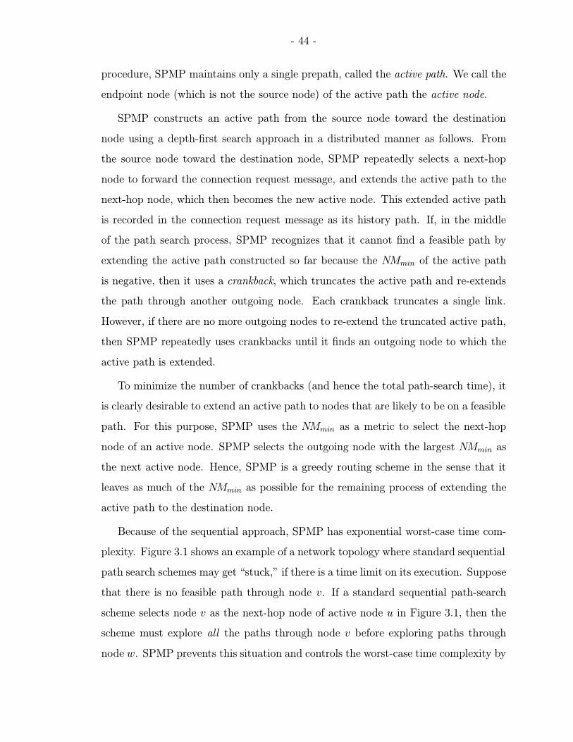
- 44 -
procedure, SPMP maintains only a single prepath, called the active path. We call the
endpoint node (which is not the source node) of the active path the active node.
SPMP constructs an active path from the source node toward the destination
node using a depth-first search approach in a distributed manner as follows. From
the source node toward the destination node, SPMP repeatedly selects a next-hop
node to forward the connection request message, and extends the active path to the
next-hop node, which then becomes the new active node. This extended active path
is recorded in the connection request message as its history path. If, in the middle
of the path search process, SPMP recognizes that it cannot find a feasible path by
extending the active path constructed so far because the NMmin of the active path
is negative, then it uses a crankback, which truncates the active path and re-extends
the path through another outgoing node. Each crankback truncates a single link.
However, if there are no more outgoing nodes to re-extend the truncated active path,
then SPMP repeatedly uses crankbacks until it finds an outgoing node to which the
active path is extended.
To minimize the number of crankbacks (and hence the total path-search time), it
is clearly desirable to extend an active path to nodes that are likely to be on a feasible
path. For this purpose, SPMP uses the NMmin as a metric to select the next-hop
node of an active node. SPMP selects the outgoing node with the largest NMmin as
the next active node. Hence, SPMP is a greedy routing scheme in the sense that it
leaves as much of the NMmin as possible for the remaining process of extending the
active path to the destination node.
Because of the sequential approach, SPMP has exponential worst-case time com-
plexity. Figure 3.1 shows an example of a network topology where standard sequential
path search schemes may get “stuck,” if there is a time limit on its execution. Suppose
that there is no feasible path through node v. If a standard sequential path-search
scheme selects node v as the next-hop node of active node u in Figure 3.1, then the
scheme must explore all the paths through node v before exploring paths through
node w. SPMP prevents this situation and controls the worst-case time complexity by
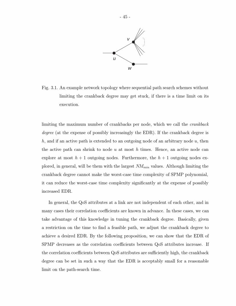
- 45 -
u
v
w
Fig. 3.1. An example network topology where sequential path search schemes without
limiting the crankback degree may get stuck, if there is a time limit on its
execution.
limiting the maximum number of crankbacks per node, which we call the crankback
degree (at the expense of possibly increasingly the EDR). If the crankback degree is
h, and if an active path is extended to an outgoing node of an arbitrary node u, then
the active path can shrink to node u at most h times. Hence, an active node can
explore at most h + 1 outgoing nodes. Furthermore, the h + 1 outgoing nodes ex-
plored, in general, will be them with the largest NMmin values. Although limiting the
crankback degree cannot make the worst-case time complexity of SPMP polynomial,
it can reduce the worst-case time complexity significantly at the expense of possibly
increased EDR.
In general, the QoS attributes at a link are not independent of each other, and in
many cases their correlation coefficients are known in advance. In these cases, we can
take advantage of this knowledge in tuning the crankback degree. Basically, given
a restriction on the time to find a feasible path, we adjust the crankback degree to
achieve a desired EDR. By the following proposition, we can show that the EDR of
SPMP decreases as the correlation coefficients between QoS attributes increase. If
the correlation coefficients between QoS attributes are sufficiently high, the crankback
degree can be set in such a way that the EDR is acceptably small for a reasonable
limit on the path-search time.
- 46 -
Proposition 3.3.1 The EDR of the proposed scheme decreases as the correlation
coefficients between QoS attributes at each link increase.
Proof Suppose that the active path has reached node u and one of its outgoing
nodes, v, has been chosen as the next-hop node. Furthermore, suppose that the ith
QoS constraint is the most stringent constraint of node v, i.e., NMmin(v) = NMi(v).
As the correlation coefficient between the ith QoS attribute and the jth QoS attribute
increases, it becomes more likely that the value of link uv with respect to the jth
QoS attribute (i.e. dj(uv)) decreases as di(uv) decreases. Thus, it also becomes more
likely that the sum of the jth QoS attribute values of the links on any postpath of
node u decreases with the sum of the ith QoS attribute values of the same links. This
increases the probability that a path satisfying the ith QoS constraint also satisfies
the jth constraint. Because the EDR decreases as the probability of finding a feasible
path increases, the EDR of SPMP decreases as the correlation coefficients between
QoS attributes increase.
3.4 SPMP: single-prepath multi-postpaths
3.4.1 SPMP algorithm
The pseudocode for SPMP is given in Figure 3.2. When a connection request
occurs, SPMP starts the routing procedure. We assume that the crankback degree
is h (e.g., for achieving a desired EDR within some run-time limit). Lines 01–07
represent the initialization procedure for the depth-first search method on lines 08–20.
Line 01–02 indicate the computations of NRs, based on (a) the routing information
provided by a distance-vector protocol in the information-advertisement process, and
(b) the constraint values included in the connection request. Lines 03–04 check if any
NR of source node s is larger than one (note that, for source node s, NRs are equal to
NMs, which SPMP uses for the eligibility test). If every NR of s is less than or equal
to one, then SPMP starts constructing the active path from s toward t by repeatedly
selecting a next-hop node in a depth-first search manner.
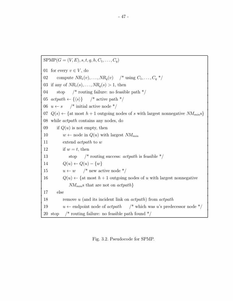
- 47 -
SPMP(G = (V,E), s, t, q, h, C1, . . . , Cq)
01 for every v ∈ V , do
02 compute NR1(v), . . . , NRq(v) /* using C1, . . . , Cq */
03 if any of NR1(s), . . . , NRq(s) > 1, then
04 stop /* routing failure: no feasible path */
05 actpath← {〈s〉} /* active path */
06 u← s /* initial active node */
07 Q(s)← {at most h+ 1 outgoing nodes of s with largest nonnegative NMmins}
08 while actpath contains any nodes, do
09 if Q(u) is not empty, then
10 w← node in Q(u) with largest NMmin
11 extend actpath to w
12 if w = t, then
13 stop /* routing success: actpath is feasible */
14 Q(u)← Q(u)− {w}
15 u← w /* new active node */
16 Q(u)← {at most h+ 1 outgoing nodes of u with largest nonnegative
NMmins that are not on actpath}
17 else
18 remove u (and its incident link on actpath) from actpath
19 u← endpoint node of actpath /* which was u’s predecessor node */
20 stop /* routing failure: no feasible path found */
Fig. 3.2. Pseudocode for SPMP.
- 48 -
To describe the depth-first search method of SPMP, suppose that SPMP has just
extended the active path from s to an arbitrary node u, and that no outgoing nodes
of u have been explored from the active path. Suppose also that u has outgoing nodes
satisfying the following two conditions: (a) the outgoing nodes are not on the active
path (to avoid loops), and (b) the path that we get by extending the active path to
each of the outgoing nodes does not have a negative NMmin. For each node u on the
active path, SPMP maintains a set Q(u) to store the outgoing nodes of u satisfying
these two conditions. If there are more than h + 1 such outgoing nodes, then only
the h+ 1 nodes with the largest NMmin values are stored in Q(u). Let node w have
the largest NMmin in Q(u).
SPMP extends the active path to node w. That is, w becomes a new active node
(lines 10–11). If w is the destination node, the routing procedure terminates because
the active path is feasible (lines 12–13). Otherwise, SPMP keeps extending the active
path by applying the following procedure. SPMP removes w from Q(u) (line 14),
updates the active node (line 15), and stores the outgoing nodes of w satisfying the
previous two conditions in the set Q(w) (line 16). If there are more than h + 1
outgoing nodes satisfying the conditions, then SPMP stores only the h + 1 nodes
with the largest NMmin values in Q(w), as in Q(u). Then, the while-loop repeats,
beginning at line 08.
Whenever SPMP explores each outgoing node of u, it is removed from Q(u).
Hence, if the number of crankbacks at u has reached the crankback degree h, or
there are no more outgoing nodes satisfying the previous two conditions, then Q(u) is
empty. In this case, the active path shrinks to the predecessor node of u (lines 17–19).
SPMP terminates the search when it finds a feasible path by extending the active
path to destination node t (lines 12–13), or cannot proceed any further (line 20).
- 49 -
3.4.2 Complexity of SPMP
If the given network topology is not of a tree structure, it is possible that the active
path leads to a node where crankbacks have occurred before. In this case, the active
path of the node is different from its old active paths (when previous crankbacks
occurred there). Because the (current) active path may indeed be part of a feasible
path, the active path should revisit the node. The possibility of such revisits to a
node makes the worst-case time complexity of the scheme exponential, as we shall
see.
Consider a graph representing a network topology for which SPMP achieves its
worst-case time complexity. If this graph is not a complete graph (where every pair of
nodes is connected by a link), then it can be extended to a complete graph by adding
links with sufficiently high QoS attribute values, such that the complete graph has the
worst-case time-complexity as well. Therefore, it suffices to consider only complete
graphs for the computation of the worst-case time complexity of SPMP. For the
time being, suppose that there is no limit on the crankback degree (i.e., exhaustive
search). When we construct an active path from a given source node at the beginning
of the routing procedure, the first next-hop node of the source node can be any node
except the source node itself (n− 1 choices), because we can use crankbacks without
restrictions. For the same reason, the second next-hop node can be any node except
the source node and the first next-hop node (n − 2 choices). Imagine continuing
this argument, until the active path reaches a given destination node. Hence, the
active path can be any path between the source and destination nodes in the network
topology, and thus the worst-case time complexity of the exhaustive search (i.e.,
SPMP without the limit on crankback degree) is (n− 1)!, which is of an exponential
form [CoL90].
We now set the crankback degree to be h to compute the worst-case time com-
plexity of SPMP. Unless all the nodes except h or fewer nodes are on the active path,
then an active node can explore at most h+1 of its outgoing nodes. The last h nodes
- 50 -
can explore at most h, h−1, . . . , 1 outgoing nodes, respectively. Thus, the worst-case
time complexity of SPMP is O((h+1)(n−h−1) ·h!). As the crankback degree decreases,
the worst-case time complexity also decreases. However, a decrease in the crankback
degree may cause an increase in the EDR as SPMP skips paths that might be feasi-
ble. Thus, we should tune the crankback degree such that both the worst-case time
complexity and the EDR are at acceptable levels.
Although the worst-case time complexity of SPMP decreases with h (i.e.,
crankback degree), it may still be impractically large even for small values of h because
of the exponential term. However, as we shall see in the next section, the average-case
time complexity of SPMP is small because of the efficient search order of SPMP (ex-
ploring the node with the largest nonnegative NMmin). When constraints are loose
(i.e., constraint values are large), it is probable that SPMP will find a feasible path
with few crankbacks. If constraints are stringent (i.e., constraint values are small),
then SPMP can skip exploring a number of paths due to negative NMmins. Therefore,
SPMP finds a feasible path or recognizes there is no feasible path in a short time. In
addition, the run time of SPMP may actually decrease as the number of constraints
increases, because the number of skipped paths (with negative NMmins) increases. In
the next section, it will be shown by simulation that the average-case time complexity
of SPMP is remarkably lower than its worst-case time complexity.
3.5 Performance evaluation
3.5.1 Generation of network topologies and QoS attribute values
To evaluate the performance of SPMP, we perform our simulation for the QoS
routing problem with two QoS attributes according to the following steps, which
are similar to those of MPLMR. First, we generate two kinds of random network
topologies, which will be described later. Next, we assign QoS attribute values to
every link in the generated network topologies. Finally, we apply SPMP for routing
in the networks. In addition, we also apply an exhaustive-search scheme to check if
- 51 -
there exists any feasible path, for the purpose of computing the EDR. We refer to a
sequence of the above steps as a simulation run. We perform 10 000 simulation runs.
To generate the two kinds of random network topologies, we use the Waxman
model [Wax88] and the Inet Topology Generator [ChC00], respectively. For each
simulation run, we generate a network topology by the Waxman model that is different
from the network topologies for previous simulation runs. This network topology is
generated as follows: source and destination nodes are located at diagonally opposite
corners of a square area of unit dimension, and then all the other nodes are spread
randomly in the square area. By the Waxman model, we introduce a link between
arbitrary nodes u and v with the following probability, which depends on the distance
between them, δ(u, v):
Pr{(u, v)} = α exp
[−δ(u, v)
β√
2
].
For the values of α and β in the above equation, we use 0.8 and 0.04, respectively,
to generate each network topology of 400 nodes. The above approach results in
approximately 1106 links per network topology. Hence, the average node degree is
5.53.
To generate the second kind of network topology, we use the Inet Topology Gen-
erator. The generated network topology has 4000 nodes and 7741 links over a square
area, and thus the average node degree is 3.87. To reduce the run-time for the gener-
ation of this large Internet-like network topology, we change source and destination
nodes randomly in the fixed network topology for all the 10 000 simulation runs,
instead of creating 10 000 network topologies. This Internet-like network topology
has smaller mean and larger variance of node degree than the network topologies
generated by the Waxman model.
Next, we assign QoS attribute values to every link using a procedure that corre-
sponds to the reverse of the “whitening process” [Fuk90]. Specifically, each link has
QoS attribute values independent of other links, and the pair of QoS attribute values
of a link has a given correlation coefficient. We assume link values for each QoS at-
tribute to have a normal distribution. For every QoS attribute, we arbitrarily assume
- 52 -
a unit mean, and set the variance as 0.16 to keep the probability of generating nega-
tive values less than 1%. When we generate a negative value, we replace it by zero.
Because very few QoS attribute values generated have zero values, link values for
each QoS attribute are still approximately normally distributed. For the constraint
value of every QoS attribute, we use 12 for the network topologies of 400 nodes, and 5
for the Internet-like network topology of 4000 nodes. These values have been chosen
such that the constraints are not too loose or too stringent. That is, these constraint
values have been chosen such that the exhaustive-search scheme just manages to find
feasible paths in most cases. The fraction of the simulation runs that have no feasible
path is approximately 10% (bigger for negative correlation coefficients and smaller
for positive correlation coefficients than this value). Recall that if constraints are too
loose or too stringent, SPMP either quickly finds a feasible path or recognizes that
there is no feasible path.
After assigning QoS attribute values, we apply the exhaustive-search scheme to
check if there exists any feasible path. Let h and ∆ be the crankback degree and the
maximum node degree of the generated network topologies, respectively. SPMP can
perform an exhaustive search by setting the crankback degree to be greater than or
equal to ∆ − 2, because every node has at most ∆ − 1 outgoing nodes (recall that
SPMP explores at most h+ 1 outgoing nodes of an active node). Then, for the same
network topology and QoS attribute values, we apply SPMP for several crankback
degrees. Finally, we ascertain whether or not there is an erroneous decision for each
scheme. Recall that an erroneous decision in this case corresponds to a failure to find
a feasible path when one exists, because we assume that all the information on a given
network topology and QoS attribute values is fixed during the routing procedure.
The average-case time complexity of SPMP is calculated based on the following
two factors: the number of computations for NRs, NMs, andNMmins, and the number
of explored nodes. When a network topology, QoS constraints, and QoS attribute
values of the links are fixed, the number of computations for NRs, NMs, and NMmins
is also fixed, and the number of explored nodes is proportional to the number of
- 53 -
crankbacks for an entire path search. Thus, we use the average number of crankbacks
for an entire path search as a metric to measure the average-case time complexity of
SPMP.
3.5.2 Simulation results
Figure 3.3 shows plots of EDR versus correlation coefficient for SPMP applied
to the network topologies of 400 nodes generated by the Waxman model and to the
Internet-like network topology of 4000 nodes. We can see that SPMP has low EDR
for all the correlation coefficients. Note that the EDR for the Internet-like network
topology is lower than for the network topologies generated by the Waxman model,
despite the larger network size. This implies that SPMP rarely misses appropriate
prepaths for each node during the course of the routing procedure. The underlying
reason is that the Internet-like network topology has smaller average node degree and
larger variance of node degree than the network topologies generated by the Waxman
model. Hence, the maximum number of crankbacks at each node (i.e., h) does not
need to be large.
In Figure 3.3, we can see that the EDR decreases rapidly with increasing crankback
degree. As mentioned before, this is possible at the expense of the exponential
worst-case time complexity. However, as shown in Figure 3.4, the average num-
ber of crankbacks for an entire path search, which we use as the measure of the
average-case time complexity for SPMP, is remarkably lower than the network size
(i.e., n or m). In addition, the average number of crankbacks for an entire path
search does not increase much as the crankback degree increases. This results from
the efficient depth-first search order, which explores first the outgoing node with the
largest NMmin, and skips exploring paths with negative NMmins.
Because SPMP has exponential worst-case time complexity, its performance when
the termination time is restricted is important. The exhaustive search scheme, which
corresponds to the SPMP with a crankback degree at least ∆ − 2 where ∆ is the
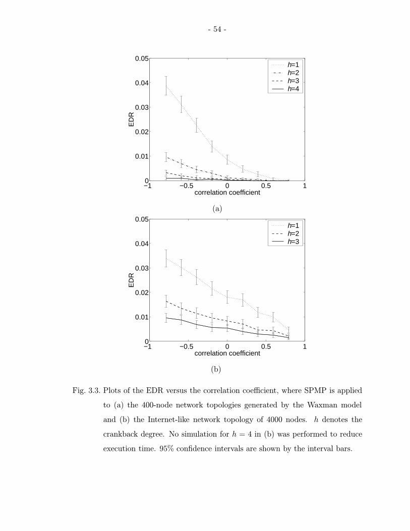
- 54 -
−1 −0.5 0 0.5 10
0.01
0.02
0.03
0.04
0.05
correlation coefficient
ED
R
h=1h=2h=3h=4
(a)
−1 −0.5 0 0.5 10
0.01
0.02
0.03
0.04
0.05
correlation coefficient
ED
R
h=1h=2h=3
(b)
Fig. 3.3. Plots of the EDR versus the correlation coefficient, where SPMP is applied
to (a) the 400-node network topologies generated by the Waxman model
and (b) the Internet-like network topology of 4000 nodes. h denotes the
crankback degree. No simulation for h = 4 in (b) was performed to reduce
execution time. 95% confidence intervals are shown by the interval bars.
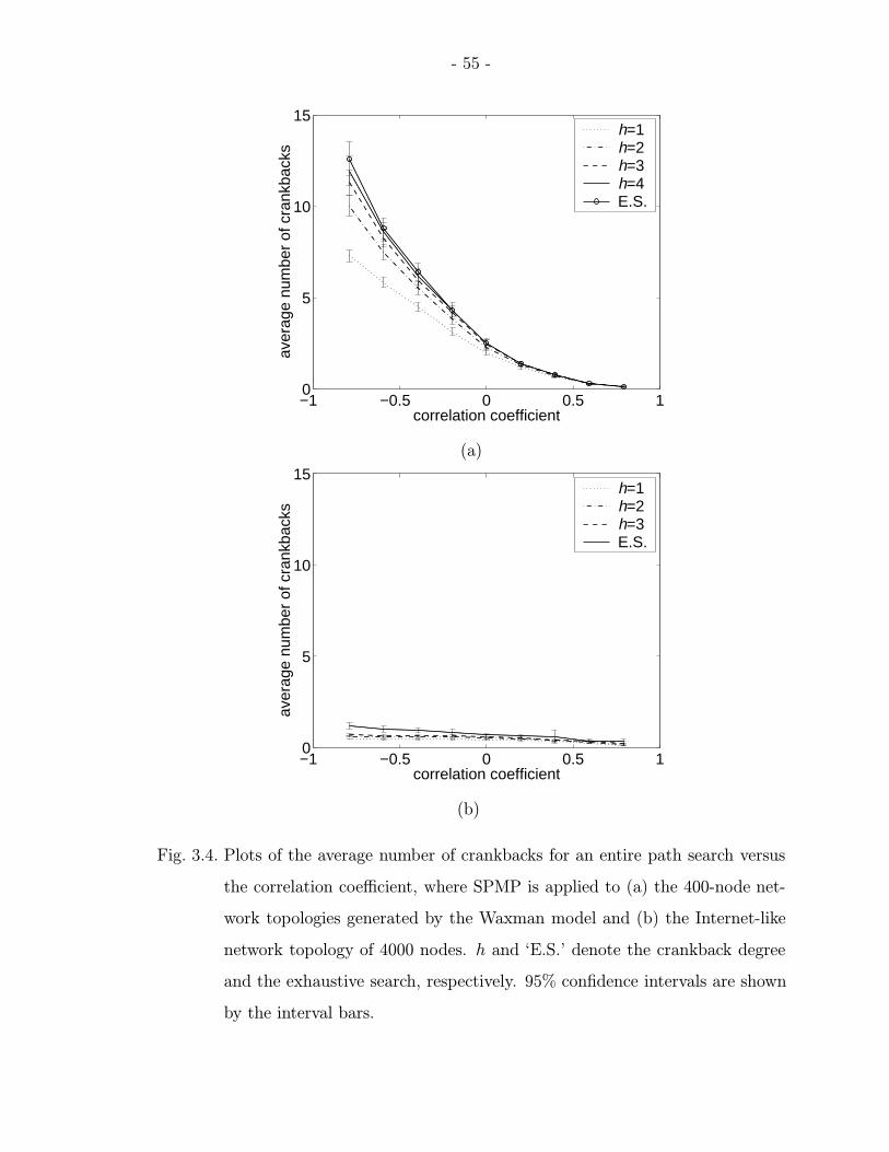
- 55 -
−1 −0.5 0 0.5 10
5
10
15
correlation coefficient
aver
age
num
ber
of c
rank
back
s
h=1h=2h=3h=4E.S.
(a)
−1 −0.5 0 0.5 10
5
10
15
correlation coefficient
aver
age
num
ber
of c
rank
back
s
h=1h=2h=3E.S.
(b)
Fig. 3.4. Plots of the average number of crankbacks for an entire path search versus
the correlation coefficient, where SPMP is applied to (a) the 400-node net-
work topologies generated by the Waxman model and (b) the Internet-like
network topology of 4000 nodes. h and ‘E.S.’ denote the crankback degree
and the exhaustive search, respectively. 95% confidence intervals are shown
by the interval bars.
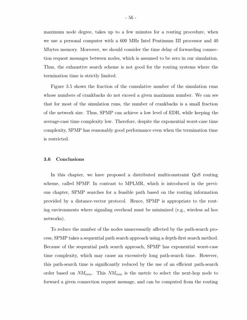
- 56 -
maximum node degree, takes up to a few minutes for a routing procedure, when
we use a personal computer with a 600 MHz Intel Pentimum III processor and 40
Mbytes memory. Moreover, we should consider the time delay of forwarding connec-
tion request messages between nodes, which is assumed to be zero in our simulation.
Thus, the exhaustive search scheme is not good for the routing systems where the
termination time is strictly limited.
Figure 3.5 shows the fraction of the cumulative number of the simulation runs
whose numbers of crankbacks do not exceed a given maximum number. We can see
that for most of the simulation runs, the number of crankbacks is a small fraction
of the network size. Thus, SPMP can achieve a low level of EDR, while keeping the
average-case time complexity low. Therefore, despite the exponential worst-case time
complexity, SPMP has reasonably good performance even when the termination time
is restricted.
3.6 Conclusions
In this chapter, we have proposed a distributed multiconstraint QoS routing
scheme, called SPMP. In contrast to MPLMR, which is introduced in the previ-
ous chapter, SPMP searches for a feasible path based on the routing information
provided by a distance-vector protocol. Hence, SPMP is appropriate to the rout-
ing environments where signaling overhead must be minimized (e.g., wireless ad hoc
networks).
To reduce the number of the nodes unnecessarily affected by the path-search pro-
cess, SPMP takes a sequential path search approach using a depth-first search method.
Because of the sequential path search approach, SPMP has exponential worst-case
time complexity, which may cause an excessively long path-search time. However,
this path-search time is significantly reduced by the use of an efficient path-search
order based on NMmin. This NMmin is the metric to select the next-hop node to
forward a given connection request message, and can be computed from the routing
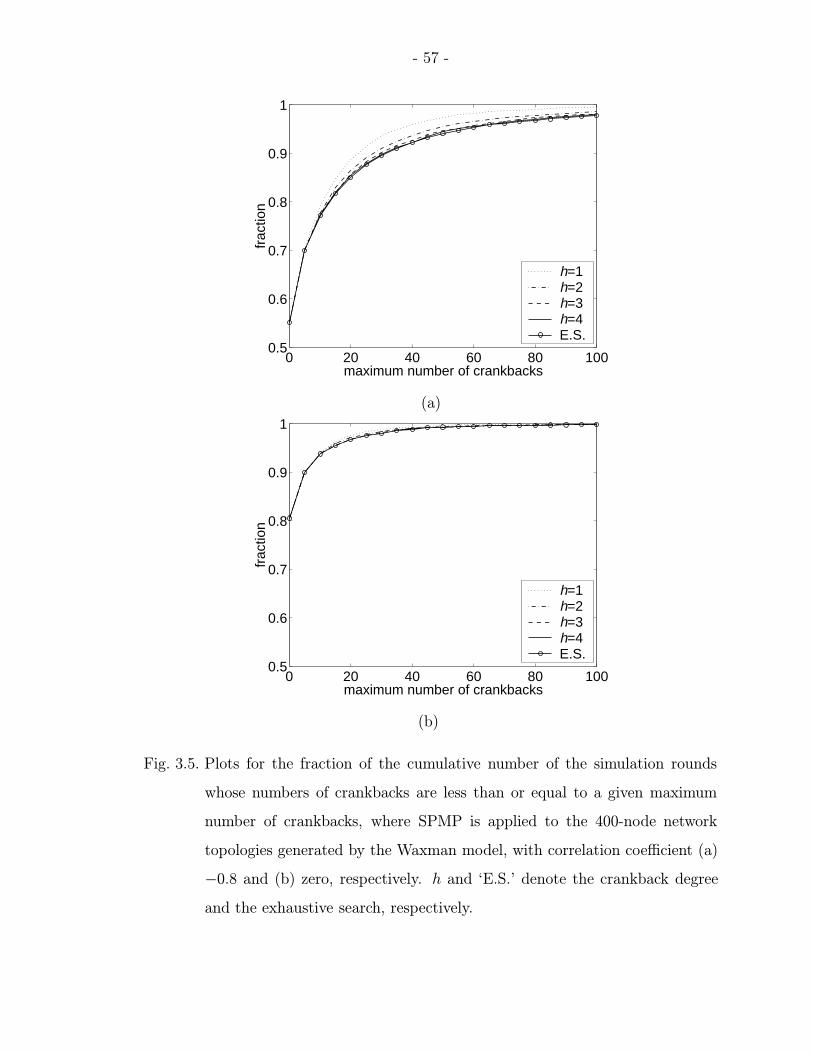
- 57 -
0 20 40 60 80 1000.5
0.6
0.7
0.8
0.9
1
maximum number of crankbacks
frac
tion
h=1h=2h=3h=4E.S.
(a)
0 20 40 60 80 1000.5
0.6
0.7
0.8
0.9
1
maximum number of crankbacks
frac
tion
h=1h=2h=3h=4E.S.
(b)
Fig. 3.5. Plots for the fraction of the cumulative number of the simulation rounds
whose numbers of crankbacks are less than or equal to a given maximum
number of crankbacks, where SPMP is applied to the 400-node network
topologies generated by the Waxman model, with correlation coefficient (a)
−0.8 and (b) zero, respectively. h and ‘E.S.’ denote the crankback degree
and the exhaustive search, respectively.
- 58 -
information provided by distance-vector protocols. Moreover, to control the path-
search time, SPMP trades off its worst-case time complexity and EDR by controlling
the crankback degree, which is the maximum number of crankbacks per node. The
efficient path-search order and the control of the crankback degree make it possible
for SPMP to keep average-case time complexity low. We showed by simulation that
SPMP also has low EDR. Hence, SPMP provides promising solutions for multicon-
straint QoS routing, which will become an essential tool in providing high-quality
services for communication/computer systems in the near future.
- 59 -
4. SURVIVABLE MULTIPATH ROUTING USING
PENALIZATION METHODS FOR WDM NETWORKS
4.1 Introduction
Wavelength division multiplexing (WDM) makes it possible to divide the huge
transmission bandwidth of an optical fiber into many wavelength channels for inde-
pendent operation of each channel. Hence, we can utilize the large bandwidth of
an optical fiber for a number of connections without the need for high-speed opto-
electronic devices. Because WDM networks offer the promise of meeting the high-
bandwidth requirements of emerging communication applications, many long-distance
carriers have already introduced point-to-point WDM transmission technologies for
their networks. However, as the number of channels accommodated on a fiber in-
creases, the following problem becomes more critical: the failure of a link can lead
to severe disruptions in many channels. Hence, survivability is a critical issue in
WDM networks. Moreover, as WDM technologies are used more widely in current
point-to-point networks, dynamic establishment of channel demands becomes more
important.
In this chapter, we address a survivable routing problem for a point-to-point con-
nection in a WDM network. The routing problem is to find a set of lightpaths
(henceforth, called paths) between a single pair of source and destination nodes on
a given physical network topology, such that the paths accommodate the requested
channels without violating the given constraints on channel demand, capacity, and
survivability. We assume that the detailed routing information of every link is known
by the use of a link-state protocol for information advertisement.
Implicitly or explicitly, many previous survivable routing schemes for WDM net-
works make two assumptions. The first assumption is that the maximum number
- 60 -
of simultaneous link failures is known (e.g., [CaP98, MoN02, RaM99, SeH02, SrR02,
ZaO03]). In most cases, at most a single link failure is assumed. The second as-
sumption is that any single path between a pair of source and destination nodes can
support all the communication traffic between the nodes. Thus, the objective of the
schemes is to make the network topology remain connected.
Based on the above assumptions, many schemes search for link-disjoint (hence-
forth, called disjoint, unless otherwise specified) paths between each pair of source
and destination nodes (e.g., [CrB98, MoN02, SeH02, ZaO03]). However, these previ-
ous schemes do not consider the vulnerability and capacity of each link. Thus, they
may require additional disjoint paths even for the connections through sufficiently
reliable paths. This requirement not only wastes network resources, but also makes
routing unnecessarily difficult. Furthermore, the schemes may not provide adequate
survivability when the number of link failures is larger than the number of disjoint
paths due to vulnerable links. Even if survivable paths are found, they may not be
able to support the communication traffic due to capacity constraints. Because of the
large bandwidth of optical fibers, previous schemes usually do not consider capacity
constraints. However, because traffic volume keeps increasing due to the continuously
growing Internet and “bandwidth-hungry” applications, it will become important to
consider capacity constraints for networks that have already been deployed.
Our goals in this chapter are to overcome the limitations of previous schemes by
considering the vulnerability and capacity of each link, and to develop survivable
routing schemes based on more general assumptions. We use failure probability as
the measure of vulnerability. We assume that each link has a given failure probability,
and that a maximum allowable failure probability for the connection between a pair
of source and destination nodes is also given (rather than assume that the maximum
number of link failures is known). We consider the capacity requirement of the con-
nection in terms of the requested number of channels, when all channels have the
same fixed bandwidth. Hence, the connection may contain several channels between
a pair of source and destination nodes, where each link has a given capacity. These
- 61 -
channels are established by a set of paths, which are not necessarily disjoint, between
the pair of source and destination nodes. Unfortunately, the development of efficient
routing schemes with all of these properties becomes hopelessly intractable as the
number of source/destination pairs increases. Hence, we limit ourselves to survivable
routing between a single pair of source and destination nodes in this chapter.
Using the maximum allowable failure probability and the requested number of
channels, we formulate a survivable routing problem for WDM networks. This prob-
lem is to find a set of paths to accommodate requested channels (and possibly addi-
tional backup channels) between a given pair of source and destination nodes, such
that the constraints on survivability and capacity are satisfied. The objective then
is to minimize the number of backup channels that allow these constraints to be
satisfied. In this problem, we do not limit routing paths to a set of disjoint paths.
As we prove in the following section, our problem is NP-hard. Hence, we develop
heuristic schemes, CPMR (conditional-penalization multipath routing) and SPMR
(successive-penalization multipath routing), for this problem.
To deal with the difficulty of allowing each link to be used for several channels,
we introduce a link penalization method. This method assigns every link a dynamic
value, called a penalty. The penalty of a link is initialized to the failure probability of
the link, and is updated to a higher value if it is determined that it is not desirable
for the link to be contained in a routing path. Using a shortest-path algorithm (e.g.,
Dijkstra’s algorithm or the Bellman-Ford algorithm) with respect to the penalty, our
schemes repeatedly select a path to accommodate a channel and add the path to the
set of selected paths. Whenever a path is selected and added, our schemes update
the penalties of the links on the selected path (before selecting the path for the next
channel). This procedure to select/add a path and update link penalties terminates
if (a) the total number of channels is at least the requested number of channels, and
(b) the probability that the number of failed channels is greater than the number of
backup channels is at most a given maximum value.
- 62 -
The procedure to update link penalties in CPMR involves a complicated compu-
tation of conditional probabilities; the scheme achieves a high routing success rate but
has a relatively long execution time. In contrast, SPMR has a simple penalty-update
procedure to reduce the execution time at the expense of a possible reduction in the
routing success rate. We show by simulation that the routing success rates of our
schemes are significantly higher than a routing scheme searching for disjoint paths,
and are almost the same as the routing success rate of a refinement to our scheme
using a simulated-annealing method, which searches for a near-optimal solution at
the expense of a much longer execution time.
The rest of this chapter is organized as follows. We discuss previous work on
survivable multipath routing for WDM networks in Section 4.2. In Section 4.3, we
present our definitions and assumptions, formulate the survivable routing problem,
and prove its NP-hardness. We summarize our approach in Section 4.4, and describe
CPMR and SPMR in detail in Sections 4.5 and 4.6, respectively. In Section 4.7, we
use simulation to evaluate and compare our schemes with the scheme searching for
disjoint paths and the scheme using simulated-annealing for a near-optimal solution.
We conclude in Section 4.8.
4.2 Previous work
Multipath routing has been used not only for survivability but also for several other
purposes, such as delay minimization (e.g., [ChC99, RoS91, Xue00]), congestion re-
duction or load balancing (e.g., [HsH01,MuG96,ZhZ02]), and security (e.g., [LoF01]).
However, as optical communication networks replace traditional high-capacity net-
works, the protection of optical communication networks against link failures has
increased the interest in multipath routing. Thus, there is a significant amount of
work on the protection of WDM networks using multipath routing capabilities.
Most previous work in survivable routing for WDM networks focuses on providing
100% protection with the assumptions that the maximum number of simultaneous
- 63 -
link failures is known, and that a single path is sufficient to cover all communication
traffic between any pair of source and destination nodes. In [MoN02], Modiano and
Tam propose a routing approach for WDM networks that performs routing on a given
physical network topology with multiple pairs of source and destination nodes. They
assume that at most a single link fails, and seek routing paths such that any single link
failure does not disconnect any pair of source and destination nodes. Although they
ignore the capacity constraint, their routing problem is still NP-complete. Hence,
they take an approach that relaxes the constraints of their routing problem to reduce
the time for finding survivable paths. Sen et al. [SeH02] consider the routing problem
with the same assumption, and propose a heuristic algorithm for routing on a given
network topology. Zang et al. [ZaO03] also deal with a similar routing problem, and
develop off-line algorithms for the protection of WDM networks under a single link
failure.
In contrast to the above papers, which deal with routing on a given network
topology, many previous papers focus on designing a survivable WDM network, but
have the same assumptions on the maximum number of link failures. Sridharan et
al. [SrS02] propose a heuristic algorithm to design a survivable WDM network with the
objective to minimize the total capacity to be consumed on all links. This algorithm
also assumes that two node-disjoint paths between each pair of source and desti-
nation nodes are sufficient to provide survivability. Caenegem et al. [CaP98] study
the techniques for routing, planning of working capacity, rerouting, and planning of
spare capacity to design a WDM network that withstands any single link failure.
Ramamurthy and Mukherjee [RaM99] investigate several approaches to protecting
WDM networks from a single link failure, and formulate a routing and wavelength
assignment problem for each approach.
Some schemes provide less stringent protection, for the sake of achieving other
goals (e.g., cost reduction). These schemes adopt similar assumptions on the maxi-
mum number of link failures and the sufficiency of a single path to cover the com-
munication traffic between any pair of source and destination nodes. Crochat and
- 64 -
Boudec [CrB98] propose a routing scheme, called the disjoint alternate path (DAP)
algorithm, which does not guarantee 100% protection for all the traffic, but minimizes
the number of source/destination pairs that would become disconnected when a single
link fails. Protection schemes that allow primary channels to share backup channels
for the efficient use of network resources are proposed in [DoD99,GhD99,HaL02]. Our
schemes differ from these in that we allow for multiple primary channels between a
given pair of source and destination nodes. In addition, we incorporate with failure
probabilities.
The assignment of failure probabilities to all failure-prone components has been
studied for general networks in several papers (e.g., [ChC95,FoS99]). However, previ-
ous problem formulations differ from ours, and thus we cannot apply these previous
schemes to our routing problem.
4.3 Survivable multipath routing problem
4.3.1 Definitions and assumptions
We first define the terminology that we will use to formulate our routing problem
and to develop our routing schemes.
• channel: a 3-tuple consisting of a source node, a destination node, and a chan-
nel bandwidth to support the communication traffic between the source and
destination nodes.
• path: a sequence of alternating nodes and links that begins and ends at nodes.
• channel realization (CR) for a given channel: a path assigned to the given
channel.
• session: a set of requested (primary) channels and extra backup channels be-
tween a given pair of source and destination nodes.
• session realization: a set of CRs for a session.

- 65 -
• session failure probability: the probability that the number of failed channels
in a session is larger than the number of backup channels in the session.
By the above definition of CR, the number of channels in a session must be the same
as the number of CRs in the corresponding session realization, but the number of
distinct paths associated with a session can be smaller than the number of channels
of the session (because several channels can be mapped to the same path). We
focus on providing “channels” between the source and destination nodes, which are
established by routing schemes that search for “paths.” Hence, we will often use
terms “CR” and “session realization” rather than terms “channel” and “session” to
show that we deal with the paths associated with the channels.
We assume the use of a link-state protocol for the advertisement of the capacity
and failure probability of each link. Hence, a network topology where every link has
an associated capacity and a failure probability is given. We consider a connection
request that contains the following information: a pair of source and destination
nodes, the number of requested (primary) channels, and the maximum allowable ses-
sion failure probability. To formulate our routing problem, we assume that the given
network topology and link values (i.e., link capacities and link failure probabilities)
are known and fixed throughout the routing procedure. We also assume that each
pair of arbitrary nodes u and v can have at most one undirected (i.e., bi-directional)
link uv between them in a given network topology (even if there are multiple fibers
between u and v, we regard them as a single link).
As is typical in the literature on survivable routing (e.g., [ChC95, MoN02]), we
are concerned only with link failures. Thus, every node is assumed to be ideal, i.e.,
have infinite capacity and zero failure probability. We assume that link failures are
independent from each other. That is, the failure of a link is assumed not to affect
the failures of other links. For simplicity, we assume that each channel takes a fixed
amount of capacity, and that we can quantify the requested capacity by the number
of channels between the source and destination nodes. In other words, each channel
is assumed to take a single unit of capacity.
- 66 -
4.3.2 Problem formulation
We wish to find a set of paths to set up a requested session with the minimum
number of channels such that the given capacity and survivability constraints are
satisfied. Henceforth, we call this routing problem the survivable multipath routing
(SMR) problem.
Definition 4.3.1 (Survivable Multipath Routing Problem) Consider an
undirected graph G = (V,E) representing a given network topology, where V and E
are sets of n nodes and m links, respectively. Suppose that each link uv has capacity
C(uv) and failure probability Pf (uv), and that the following are given: source node s,
destination node t, requested number of channels N , and maximum allowable session
failure probability PMASF . Find a session realization X with the smallest number of
channels, such that the following three conditions are satisfied. (a) The total number
of channels is at least N . (b) The number of channels accommodated in each link
does not exceed the capacity of the link. (c) The session failure probability of X does
not exceed PMASF .
Consider session realization X consisting of L CRs x1, . . . , xL, where M of them
are for backup channels. That is,
L = N +M. (4.1)
Let A(uv) be the number of channels accommodated in link uv, HL = {1, . . . , L},
and P (x(F )j1, . . . , x
(F )jk, x
(W )jk+1
, . . . , x(W )jL
) be the probability that CRs xj1 , . . . , xjk fail and
CRs xjk+1, . . . , xjL work. The probability that any k of the L CRs in X fail, denoted
by P (X,L, k), is represented as follows:
P (X,L, k) =∑
{j1,...,jk}⊂HL,{jk+1,...,jL}=HL−{j1,...,jk}
P (x(F )j1, . . . , x
(F )jk, x
(W )jk+1
, . . . , x(W )jL
). (4.2)
- 67 -
For the summation, the first set {j1, . . . , jk} ⊂ HL represents all possible subsets of
k failed channels. We describe how to compute P (X,L, k) of (4.2) in Appendix A.
Using (4.2), we can represent the session failure probability of X as follows:
Pf(X) =L∑
k=M+1
P (X,L, k). (4.3)
Now, we can restate the SMR problem as follows: Given the setup of the SMR
problem, find a session realization X = {x1, x2, . . . , xL} that minimizes L subject to
the following inequalities:
L ≥ N, (4.4)
A(uv) ≤ C(uv) for every uv ∈ E, and (4.5)
Pf(X) ≤ PMASF . (4.6)
Equations (4.4), (4.5), and (4.6) represent the constraints on channel demand, capac-
ity, and survivability, respectively. A session realization is feasible if it satisfies (4.4),
(4.5), and (4.6).
Theorem 4.3.1 The SMR problem is NP-hard.
Proof To show that the SMR problem is NP-hard, we reduce the “k link-disjoint
paths” problem (henceforth, k-LDP problem) to the SMR problem. Given an undi-
rected graph with k pairs of source and destination nodes (si, ti) for i = 1, . . . , k, the
k-LDP problem is to find a path between si and ti for every i = 1, . . . , k such that no
two paths share a link. This is a well-known NP-complete problem [Fra90].
To reduce the k-LDP problem to the SMR problem, we form a new graph for the
SMR problem from the graph of the k-LDP problem in the following procedure, as
illustrated in Figure 4.1. First, we add source and destination nodes s and t. We
then add a unique node ui between s and si, and a unique node vi between ti and t
for i = 1, . . . , k. That is, if i 6= j, then ui and uj (or vi and vj) are distinct nodes.
Note that, in contrast, any node si (or ti) may be used for several pairs of source and
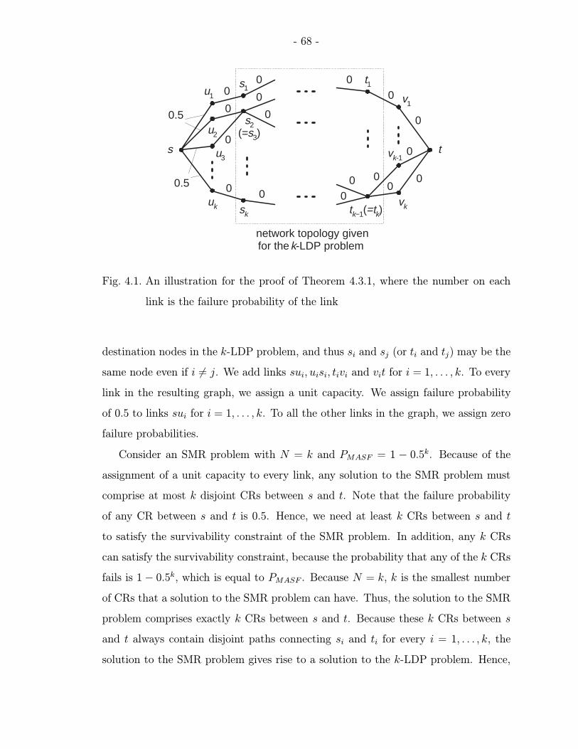
- 68 -
s t
0
00 0
0
0
0
0.5
s1
s2(=s3)
sk
t1
tk−1(=tk)
0
00
0
0
0
00.5
0
00
u1
u2
u3
uk
v1
vk-1
vk
network topology givenfor the k-LDP problem
Fig. 4.1. An illustration for the proof of Theorem 4.3.1, where the number on each
link is the failure probability of the link
destination nodes in the k-LDP problem, and thus si and sj (or ti and tj) may be the
same node even if i 6= j. We add links sui, uisi, tivi and vit for i = 1, . . . , k. To every
link in the resulting graph, we assign a unit capacity. We assign failure probability
of 0.5 to links sui for i = 1, . . . , k. To all the other links in the graph, we assign zero
failure probabilities.
Consider an SMR problem with N = k and PMASF = 1 − 0.5k. Because of the
assignment of a unit capacity to every link, any solution to the SMR problem must
comprise at most k disjoint CRs between s and t. Note that the failure probability
of any CR between s and t is 0.5. Hence, we need at least k CRs between s and t
to satisfy the survivability constraint of the SMR problem. In addition, any k CRs
can satisfy the survivability constraint, because the probability that any of the k CRs
fails is 1− 0.5k, which is equal to PMASF . Because N = k, k is the smallest number
of CRs that a solution to the SMR problem can have. Thus, the solution to the SMR
problem comprises exactly k CRs between s and t. Because these k CRs between s
and t always contain disjoint paths connecting si and ti for every i = 1, . . . , k, the
solution to the SMR problem gives rise to a solution to the k-LDP problem. Hence,
- 69 -
the k-LDP problem is solvable if the SMR problem is solvable. Finally, it is easy to
see that this reduction takes polynomial time.
4.4 Elements of the proposed routing techniques
4.4.1 Link penalization
In this section, we focus on the survivability constraint. To find a feasible session
realization, our basic approach is to repeatedly add a channel to the session (and
select a CR for the channel and add it to the corresponding session realization).
Each time we add a channel to a session, the session failure probability decreases or
does not change. We repeat the procedure of adding a channel one-by-one, until the
session failure probability falls below PMASF or no more channels can be realized due
to the capacity limit between the source and destination nodes. Because our goal is
to minimize the number of channels in the session, it is important to select CRs of
low path failure probabilities for lowering the session failure probability. Hence, CRs
should contain links of low failure probabilities. However, our schemes allow each
link to be used for several channels, and thus several CRs may share a link with low
failure probability. This may cause a high session failure probability even though the
link failure probability is low, because several channels will fail together if the shared
link fails. Therefore, we need to control (but, not prohibit) link-sharing.
To control link-sharing, our approach is to assign every link a dynamic value,
called a penalty. The penalty of a link is initially equal to the failure probability of
the link. We repeatedly select a CR using a shortest-path algorithm with respect
to the penalty and update the penalties of the links on the selected CR before the
selection of the next CR. The penalty of a link must be set to a high value if it is
not desirable for the link to be contained in a CR. Hence, if a link shared by several
CRs causes the session to be vulnerable to failure, the penalty of the link must be
increased. That is, we may have to increase the penalties of the links on CRs to
penalize the selection of the links for other CRs. Details on how to increase the link
- 70 -
penalties will be described in the following sections (CPMR and SPMR use different
methods for setting penalty values).
Penalties and failure probabilities share some common properties. Specifically,
the penalty values are always in [0,1], and the penalty of a CR is defined from the
penalties of the links on the CR in the same way that the failure probability of a path
is computed from the failure probabilities of the links on the path. Let PN(x) be the
penalty of CR x, E(x) the set of all the links on x, and PN(uv) the penalty of link
uv. Then,
PN(x) = 1−∏
uv∈E(x)
[ 1− PN(uv) ]. (4.7)
For finding the first CR, we set the penalty of each link to be equal to its failure
probability, and then select the path that has the smallest penalty. If the session
realization containing only this CR does not satisfy the constraints of (4.4) and (4.6),
then we repeat the following procedure until these constraints are satisfied or no more
CRs can be found due to the capacity limit between source and destination nodes:
(i) update the penalties of the links on the CR just selected (described later), (ii)
select a new CR with the smallest penalty to add into the session realization, and
(iii) compute the session failure probability to check if the survivability constraint is
satisfied.
4.4.2 Residual networks and link cancellation
In this section, we focus on the capacity constraint. To find a session real-
ization satisfying the capacity constraint, we use the notions of residual networks
and link cancellation, which were originally introduced for the maximum flow prob-
lem [AhM93,CoL90]. To apply the idea of residual networks to our problem, convert
the given undirected graph G to a corresponding directed graph D1 by replacing
each undirected link uv with a pair of directed links with opposite directions, i.e.,
−→uv and −→vu. These links −→uv and −→vu are assigned the same failure probability as link
uv, and they always have the same penalty. Then, perform a routing procedure on
- 71 -
this directed graph. After finishing the routing procedure, reconvert directed links to
undirected links.
For an arbitrary undirected link uv in G, each of directed links −→uv and −→vu in D1
initially has the same capacity that uv has. After selecting the first CR x1 in D1, if
we need more CRs for a feasible session realization, we compute the residual network
with respect to the selected CR, denoted by D2. In D2, every directed link −→uv on x1
has capacity smaller by one than in D1, and the reverse link −→vu has capacity larger by
one than in D1. We repeat this procedure (i.e., selection of a CR and computation of
the residual network) until the session realization becomes feasible or no more CRs
can be found due to the capacity limit between source and destination nodes.
Example residual networks are shown in Figure 4.2. Suppose that we are given
undirected graph G in Figure 4.2(a). The number on each link represents the capacity
of the link. D1 in Figure 4.2(b) is the directed graph that corresponds to G. Suppose
also that we set up CR x1 = 〈s, u, v, t〉 in D1. Then, as is shown in Figure 4.2(c),
the capacities of (forward) links −→su,−→uv, and−→vt decrease by one, respectively, in the
residual network of D1 with respect to x1, denoted by D2, and the capacities of the
reverse links −→us,−→vu, and−→tv increase by one, respectively, in D2.
The increase in the capacities of reverse links in a residual network represents
the possibility of link cancellation. For example, consider a pair of directed links
with opposite directions (i.e., −→uv and −→vu). The operation of link cancellation involves
replacing the two CRs containing−→uv and −→vu respectively, with two new CRs as follows:
first remove the two opposite links from the two given CRs, and then swap the
subpaths after these links. This results in two new CRs between the source and
destination nodes. Figure 4.2(d) shows this example that CRs x1 and x2 change
to new CRs x′1 and x′2 by link cancellation. The use of residual networks with link
cancellation makes it possible to add CRs into a session realization up to the capacity
limit between the source and destination nodes, even though the selected CRs have
already occupied links that would bottleneck the addition of new CRs.
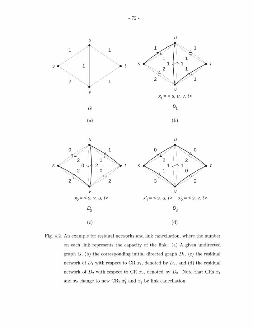
- 72 -
s t
1
1
2
1
1
G
u
v
s t
1
1
2
211
1
1
1
1
D1
u
vx1 = < s, u, v, t >
(a) (b)
s t
0
2
2
220
1
1
0
2
u
v
D2
x2 = < s, v, u, t >
s t
0
2
3
111
0
2
0
2
D3
u
vx'1 = < s, u, t > x'2 = < s, v, t >
(c) (d)
Fig. 4.2. An example for residual networks and link cancellation, where the number
on each link represents the capacity of the link. (a) A given undirected
graph G, (b) the corresponding initial directed graph D1, (c) the residual
network of D1 with respect to CR x1, denoted by D2, and (d) the residual
network of D2 with respect to CR x2, denoted by D3. Note that CRs x1
and x2 change to new CRs x′1 and x′2 by link cancellation.
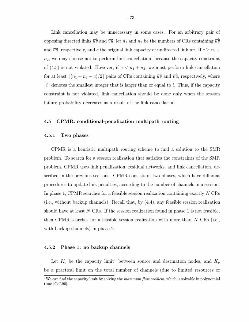
- 73 -
Link cancellation may be unnecessary in some cases. For an arbitrary pair of
opposing directed links −→uv and −→vu, let n1 and n2 be the numbers of CRs containing −→uv
and −→vu, respectively, and c the original link capacity of undirected link uv. If c ≥ n1 +
n2, we may choose not to perform link cancellation, because the capacity constraint
of (4.5) is not violated. However, if c < n1 + n2, we must perform link cancellation
for at least d(n1 + n2 − c)/2e pairs of CRs containing −→uv and −→vu, respectively, where
die denotes the smallest integer that is larger than or equal to i. Thus, if the capacity
constraint is not violated, link cancellation should be done only when the session
failure probability decreases as a result of the link cancellation.
4.5 CPMR: conditional-penalization multipath routing
4.5.1 Two phases
CPMR is a heuristic multipath routing scheme to find a solution to the SMR
problem. To search for a session realization that satisfies the constraints of the SMR
problem, CPMR uses link penalization, residual networks, and link cancellation, de-
scribed in the previous sections. CPMR consists of two phases, which have different
procedures to update link penalties, according to the number of channels in a session.
In phase 1, CPMR searches for a feasible session realization containing exactly N CRs
(i.e., without backup channels). Recall that, by (4.4), any feasible session realization
should have at least N CRs. If the session realization found in phase 1 is not feasible,
then CPMR searches for a feasible session realization with more than N CRs (i.e.,
with backup channels) in phase 2.
4.5.2 Phase 1: no backup channels
Let Kc be the capacity limit1 between source and destination nodes, and Kp
be a practical limit on the total number of channels (due to limited resources or
1We can find the capacity limit by solving the maximum flow problem, which is solvable in polynomialtime [CoL90].
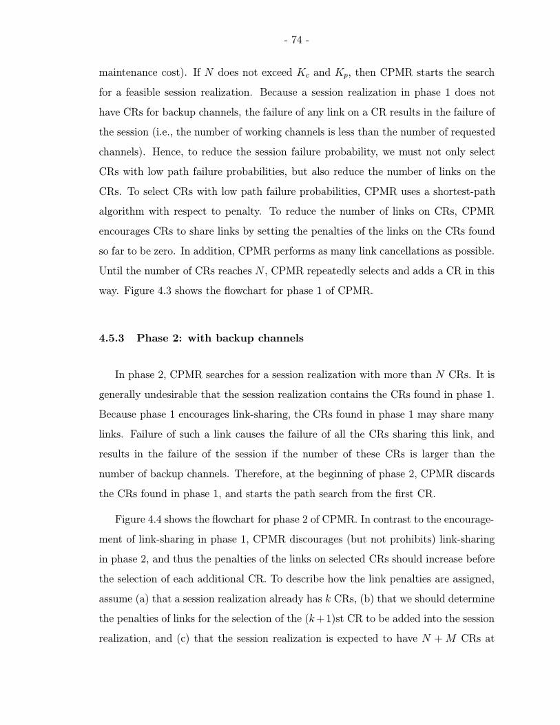
- 74 -
maintenance cost). If N does not exceed Kc and Kp, then CPMR starts the search
for a feasible session realization. Because a session realization in phase 1 does not
have CRs for backup channels, the failure of any link on a CR results in the failure of
the session (i.e., the number of working channels is less than the number of requested
channels). Hence, to reduce the session failure probability, we must not only select
CRs with low path failure probabilities, but also reduce the number of links on the
CRs. To select CRs with low path failure probabilities, CPMR uses a shortest-path
algorithm with respect to penalty. To reduce the number of links on CRs, CPMR
encourages CRs to share links by setting the penalties of the links on the CRs found
so far to be zero. In addition, CPMR performs as many link cancellations as possible.
Until the number of CRs reaches N , CPMR repeatedly selects and adds a CR in this
way. Figure 4.3 shows the flowchart for phase 1 of CPMR.
4.5.3 Phase 2: with backup channels
In phase 2, CPMR searches for a session realization with more than N CRs. It is
generally undesirable that the session realization contains the CRs found in phase 1.
Because phase 1 encourages link-sharing, the CRs found in phase 1 may share many
links. Failure of such a link causes the failure of all the CRs sharing this link, and
results in the failure of the session if the number of these CRs is larger than the
number of backup channels. Therefore, at the beginning of phase 2, CPMR discards
the CRs found in phase 1, and starts the path search from the first CR.
Figure 4.4 shows the flowchart for phase 2 of CPMR. In contrast to the encourage-
ment of link-sharing in phase 1, CPMR discourages (but not prohibits) link-sharing
in phase 2, and thus the penalties of the links on selected CRs should increase before
the selection of each additional CR. To describe how the link penalties are assigned,
assume (a) that a session realization already has k CRs, (b) that we should determine
the penalties of links for the selection of the (k+1)st CR to be added into the session
realization, and (c) that the session realization is expected to have N + M CRs at
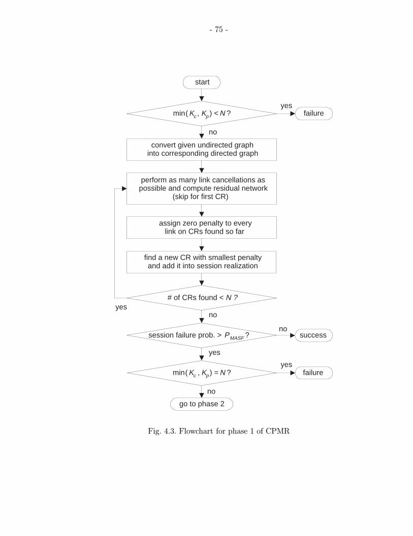
- 75 -
# of CRs found < N ?
noyes
min ( Kc , Kp ) < N ?yes
yes
go to phase 2
assign zero penalty to everylink on CRs found so far
perform as many link cancellations aspossible and compute residual network
(skip for first CR)
session failure prob. > P MASF ?
start
convert given undirected graphinto corresponding directed graph
successno
failure
no
find a new CR with smallest penaltyand add it into session realization
yesmin ( Kc , Kp ) = N ? failure
no
Fig. 4.3. Flowchart for phase 1 of CPMR
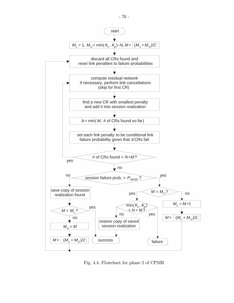
- 76 -
M = (M L + M U )/2
# of CRs found < N +M ?
no
yes
yes
set each link penalty to be conditional linkfailure probability given that b CRs fail
compute residual networkif necessary, perform link cancellations
(skip for first CR)
session failure prob. > P MASF ?
start
M L = 1, M U = min ( Kc , Kp )−N, M = (M L + M U )/2
success
b = min ( M , # of CRs found so far )
discard all CRs found andreset link penalties to failure probabilities
M L = M +1yes
M U = M
no
no
M = M L ?
M = M U ? no
M = (M L + M U )/2
find a new CR with smallest penaltyand add it into session realization
yes
no
min ( Kc , Kp )= N + M ?
failure
yes
save copy of sessionrealization found
restore copy of savedsession realization
Fig. 4.4. Flowchart for phase 2 of CPMR
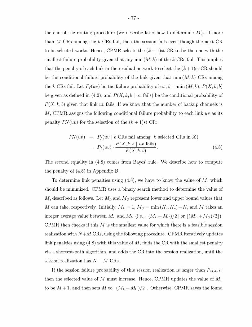
- 77 -
the end of the routing procedure (we describe later how to determine M). If more
than M CRs among the k CRs fail, then the session fails even though the next CR
to be selected works. Hence, CPMR selects the (k + 1)st CR to be the one with the
smallest failure probability given that any min (M, k) of the k CRs fail. This implies
that the penalty of each link in the residual network to select the (k+1)st CR should
be the conditional failure probability of the link given that min (M, k) CRs among
the k CRs fail. Let Pf(uv) be the failure probability of uv, b = min (M, k), P (X, k, b)
be given as defined in (4.2), and P (X, k, b | uv fails) be the conditional probability of
P (X, k, b) given that link uv fails. If we know that the number of backup channels is
M , CPMR assigns the following conditional failure probability to each link uv as its
penalty PN(uv) for the selection of the (k + 1)st CR:
PN(uv) = Pf(uv | b CRs fail among k selected CRs in X)
= Pf(uv) ·P (X, k, b | uv fails)
P (X, k, b). (4.8)
The second equality in (4.8) comes from Bayes’ rule. We describe how to compute
the penalty of (4.8) in Appendix B.
To determine link penalties using (4.8), we have to know the value of M , which
should be minimized. CPMR uses a binary search method to determine the value of
M , described as follows. Let ML andMU represent lower and upper bound values that
M can take, respectively. Initially, ML = 1, MU = min (Kc, Kp)−N , and M takes an
integer average value between ML and MU (i.e., d(ML +MU)/2e or b(ML +MU)/2c).
CPMR then checks if this M is the smallest value for which there is a feasible session
realization with N+M CRs, using the following procedure. CPMR iteratively updates
link penalties using (4.8) with this value of M , finds the CR with the smallest penalty
via a shortest-path algorithm, and adds the CR into the session realization, until the
session realization has N +M CRs.
If the session failure probability of this session realization is larger than PMASF ,
then the selected value of M must increase. Hence, CPMR updates the value of ML
to be M + 1, and then sets M to d(ML +MU)/2e. Otherwise, CPMR saves the found
- 78 -
(feasible) session realization, updates the value of MU to be M , and then decreases
M to b(ML +MU)/2c. When M increases or decreases, CPMR discards all the CRs
found and repeats the above procedure. This binary search process terminates when
M = MU and the session failure probability is larger than PMASF , or when M = ML
and the session failure probability is smaller than or equal to PMASF . The output
of phase 2 is the feasible session realization saved lastly or the infeasible session
realization with the min (Kc, Kp) CRs produced by the binary search method. In
phase 2, link cancellation occurs only when the session failure probability decreases,
or when the cancellations are mandatory due to the capacity constraint of (4.5).
4.5.4 Complexity of CPMR
The complexity of CPMR is dependent on the number of channels in a session (i.e.,
L in (4.1)). If we do not limit the number of channels, then the possible number of
channels between a given pair of source and destination nodes may increase exponen-
tially with the number of nodes (or links). Thus, CPMR has exponential complexity
with respect to the network size (i.e., the number of nodes or links). Specifically, the
exponential complexity of CPMR comes from the following factors: (a) the compu-
tation of the session failure probability in (4.3), (b) the search for opposing links for
which link cancellation should be performed, and (c) the update of link penalties by
(4.8).
First, the computation of the session failure probability is inevitable to check if the
survivability constraint is satisfied. As described in Appendix A, we may reduce this
computation time2 if the number of channels is small, which is typical in practical
situations. Next, the procedure to search for opposing links for link cancellation
does not affect the execution time significantly because CPMR uses a shortest-path
algorithm to select CRs. If a CR x that contains an arbitrary link −→uv is “short” (i.e.,
2There are several studies on efficient algorithms to compute network reliability, which can be usedfor the computation of the session failure probability (e.g., [SiG94]). However, the development ofefficient algorithms to compute the session failure probability is beyond the scope of this research.We used the computation method introduced in Appendix A for our simulation in Section 4.7.
- 79 -
of low path failure probability), then another CR containing −→vu is likely to be “long”
compared to x because the −→vu is not likely to be directed toward the destination
node. Hence, few CRs in a session realization are likely to contain opposing links,
and thus link cancellation rarely occurs. Last, we can compute the conditional failure
probability of (4.8) in a similar way that we compute the session failure probability
(see Appendix B). The update of all the penalties of the links on a newly added CR has
the same complexity as the computation of the session failure probability. Therefore,
if the total number of channels in the session is small, then the exponential complexity
of CPMR is not likely to result in a prohibitively long execution time. In contrast
to the previous two factors (one of which is inevitable and the other occurs rarely),
we can reduce the effect of the third factor on the execution time by updating link
penalties in a simpler way. This is the basic idea of SPMR, which is described in the
next section.
4.6 SPMR: successive-penalization multipath routing
SPMR is a simplified version of CPMR. SPMR also consists of two phases, and
phase 1 of SPMR is the same as phase 1 of CPMR. However, phase 2 of SPMR has a
different procedure to update link penalties. Recall that in phase 2, CPMR predicts
a value of M , and based on this value, computes the conditional failure probability
of (4.8) to update link penalties. However, SPMR updates link penalties in a simpler
way, and thus reduces the run-time at the expense of a possible increase in the number
of backup channels.
Figure 4.5 shows the flowchart for phase 2 of SPMR. As in CPMR, SPMR dis-
courages link-sharing in phase 2. If no link cancellation occurs, SPMR updates link
penalties as follows. Let x be the CR just found, E(x) the set of links on x, PNo(uv)
the old penalty of link uv ∈ E(x) (which has been used to find x), PNo(x) the old
penalty of x (which is computed from the old penalties of the links on x), and PNn(uv)
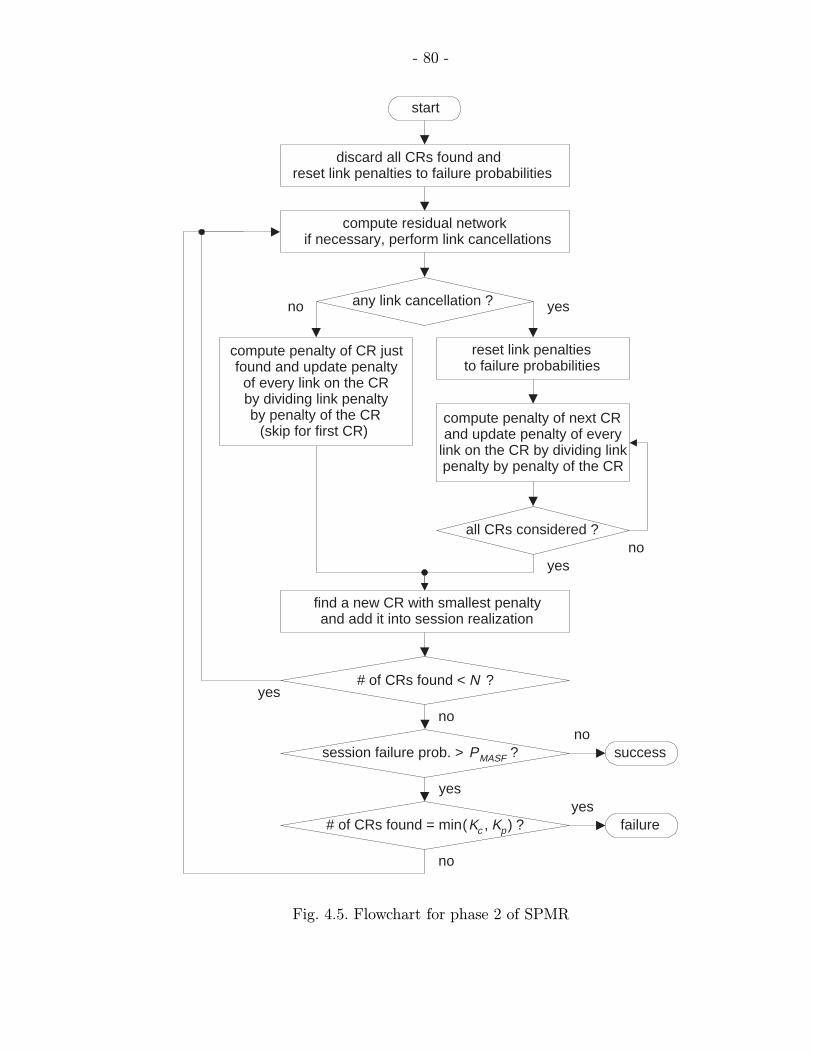
- 80 -
# of CRs found < N ?yes
compute residual networkif necessary, perform link cancellations
session failure prob. > P MASF ?
start
success
discard all CRs found andreset link penalties to failure probabilities
yes
nono
find a new CR with smallest penaltyand add it into session realization
# of CRs found = min ( Kc , Kp ) ?
no
failureyes
any link cancellation ? yesno
compute penalty of CR justfound and update penalty
of every link on the CRby dividing link penaltyby penalty of the CR
(skip for first CR)compute penalty of next CRand update penalty of every
link on the CR by dividing linkpenalty by penalty of the CR
all CRs considered ?
yesno
reset link penaltiesto failure probabilities
Fig. 4.5. Flowchart for phase 2 of SPMR
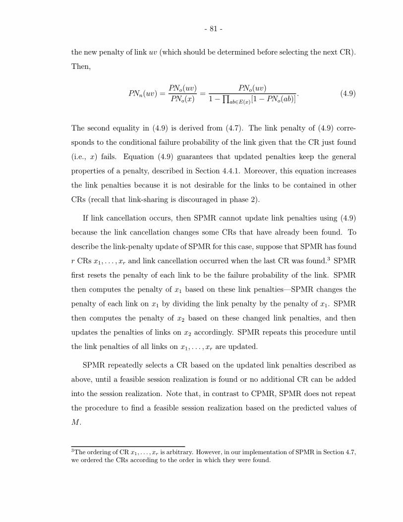
- 81 -
the new penalty of link uv (which should be determined before selecting the next CR).
Then,
PNn(uv) =PNo(uv)
PNo(x)=
PNo(uv)
1−∏
ab∈E(x)[1− PNo(ab)]. (4.9)
The second equality in (4.9) is derived from (4.7). The link penalty of (4.9) corre-
sponds to the conditional failure probability of the link given that the CR just found
(i.e., x) fails. Equation (4.9) guarantees that updated penalties keep the general
properties of a penalty, described in Section 4.4.1. Moreover, this equation increases
the link penalties because it is not desirable for the links to be contained in other
CRs (recall that link-sharing is discouraged in phase 2).
If link cancellation occurs, then SPMR cannot update link penalties using (4.9)
because the link cancellation changes some CRs that have already been found. To
describe the link-penalty update of SPMR for this case, suppose that SPMR has found
r CRs x1, . . . , xr and link cancellation occurred when the last CR was found.3 SPMR
first resets the penalty of each link to be the failure probability of the link. SPMR
then computes the penalty of x1 based on these link penalties—SPMR changes the
penalty of each link on x1 by dividing the link penalty by the penalty of x1. SPMR
then computes the penalty of x2 based on these changed link penalties, and then
updates the penalties of links on x2 accordingly. SPMR repeats this procedure until
the link penalties of all links on x1, . . . , xr are updated.
SPMR repeatedly selects a CR based on the updated link penalties described as
above, until a feasible session realization is found or no additional CR can be added
into the session realization. Note that, in contrast to CPMR, SPMR does not repeat
the procedure to find a feasible session realization based on the predicted values of
M .
3The ordering of CR x1, . . . , xr is arbitrary. However, in our implementation of SPMR in Section 4.7,we ordered the CRs according to the order in which they were found.
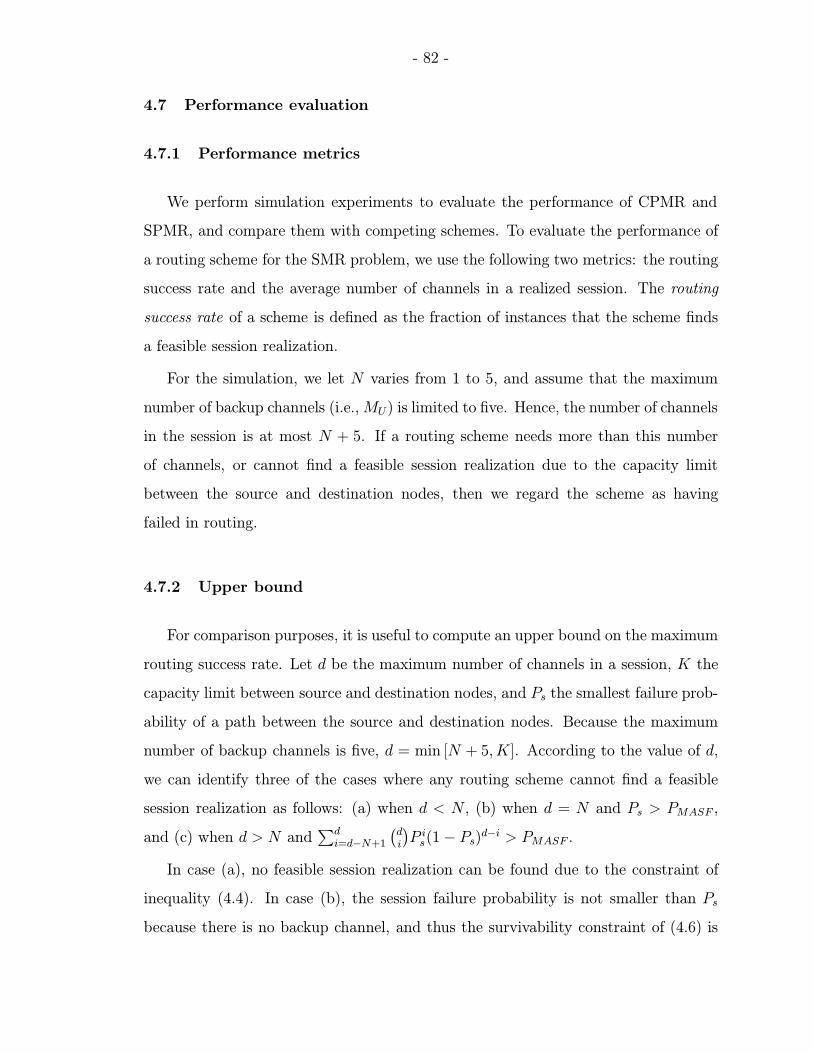
- 82 -
4.7 Performance evaluation
4.7.1 Performance metrics
We perform simulation experiments to evaluate the performance of CPMR and
SPMR, and compare them with competing schemes. To evaluate the performance of
a routing scheme for the SMR problem, we use the following two metrics: the routing
success rate and the average number of channels in a realized session. The routing
success rate of a scheme is defined as the fraction of instances that the scheme finds
a feasible session realization.
For the simulation, we let N varies from 1 to 5, and assume that the maximum
number of backup channels (i.e., MU) is limited to five. Hence, the number of channels
in the session is at most N + 5. If a routing scheme needs more than this number
of channels, or cannot find a feasible session realization due to the capacity limit
between the source and destination nodes, then we regard the scheme as having
failed in routing.
4.7.2 Upper bound
For comparison purposes, it is useful to compute an upper bound on the maximum
routing success rate. Let d be the maximum number of channels in a session, K the
capacity limit between source and destination nodes, and Ps the smallest failure prob-
ability of a path between the source and destination nodes. Because the maximum
number of backup channels is five, d = min [N + 5, K]. According to the value of d,
we can identify three of the cases where any routing scheme cannot find a feasible
session realization as follows: (a) when d < N , (b) when d = N and Ps > PMASF ,
and (c) when d > N and∑d
i=d−N+1
(di
)P is(1− Ps)
d−i > PMASF .
In case (a), no feasible session realization can be found due to the constraint of
inequality (4.4). In case (b), the session failure probability is not smaller than Ps
because there is no backup channel, and thus the survivability constraint of (4.6) is
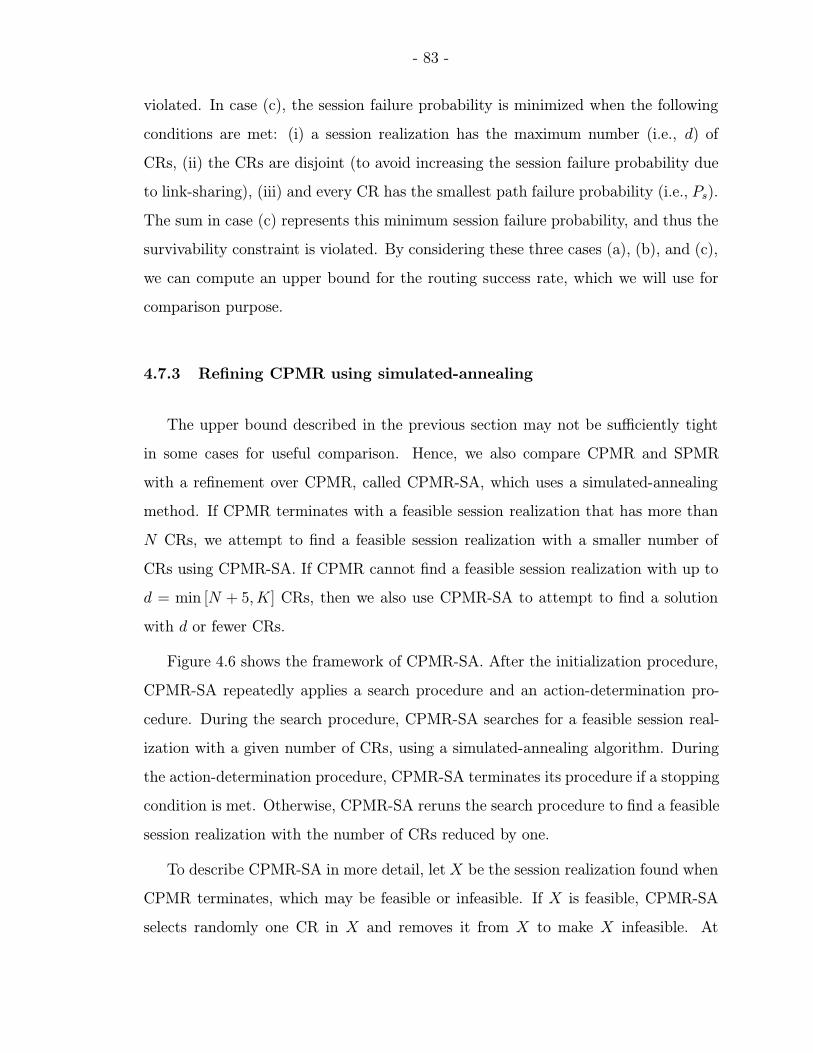
- 83 -
violated. In case (c), the session failure probability is minimized when the following
conditions are met: (i) a session realization has the maximum number (i.e., d) of
CRs, (ii) the CRs are disjoint (to avoid increasing the session failure probability due
to link-sharing), (iii) and every CR has the smallest path failure probability (i.e., Ps).
The sum in case (c) represents this minimum session failure probability, and thus the
survivability constraint is violated. By considering these three cases (a), (b), and (c),
we can compute an upper bound for the routing success rate, which we will use for
comparison purpose.
4.7.3 Refining CPMR using simulated-annealing
The upper bound described in the previous section may not be sufficiently tight
in some cases for useful comparison. Hence, we also compare CPMR and SPMR
with a refinement over CPMR, called CPMR-SA, which uses a simulated-annealing
method. If CPMR terminates with a feasible session realization that has more than
N CRs, we attempt to find a feasible session realization with a smaller number of
CRs using CPMR-SA. If CPMR cannot find a feasible session realization with up to
d = min [N + 5, K] CRs, then we also use CPMR-SA to attempt to find a solution
with d or fewer CRs.
Figure 4.6 shows the framework of CPMR-SA. After the initialization procedure,
CPMR-SA repeatedly applies a search procedure and an action-determination pro-
cedure. During the search procedure, CPMR-SA searches for a feasible session real-
ization with a given number of CRs, using a simulated-annealing algorithm. During
the action-determination procedure, CPMR-SA terminates its procedure if a stopping
condition is met. Otherwise, CPMR-SA reruns the search procedure to find a feasible
session realization with the number of CRs reduced by one.
To describe CPMR-SA in more detail, let X be the session realization found when
CPMR terminates, which may be feasible or infeasible. If X is feasible, CPMR-SA
selects randomly one CR in X and removes it from X to make X infeasible. At
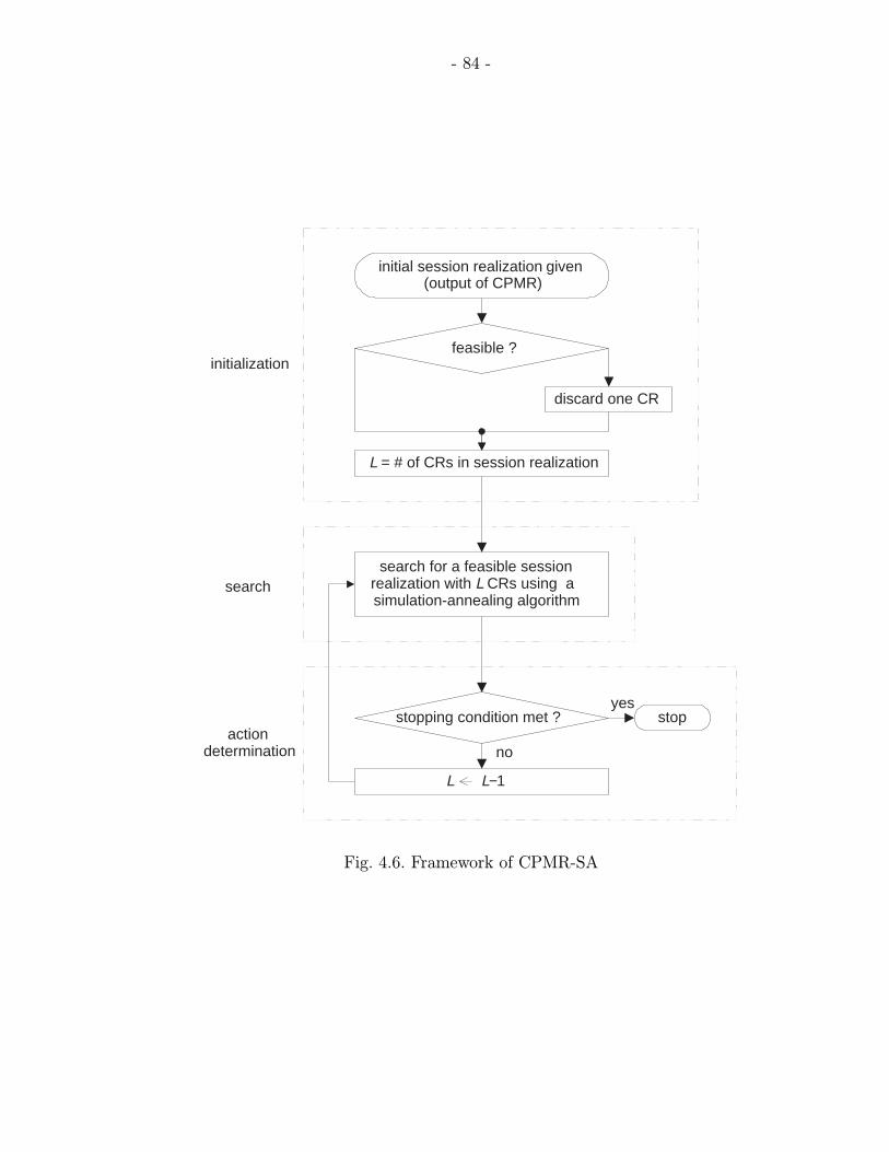
- 84 -
yes
search for a feasible sessionrealization with L CRs using asimulation-annealing algorithm
initial session realization given(output of CPMR)
stop
no
L L−1
actiondetermination
search
stopping condition met ?
feasible ?
discard one CR
L = # of CRs in session realization
initialization
Fig. 4.6. Framework of CPMR-SA

- 85 -
this point, either X was originally infeasible, or has been changed to be infeasible.
Suppose that X now has L CRs. Now, the search procedure of CPMR-SA attempts to
find a feasible session realization with L CRs, using a simulated-annealing algorithm
as follows.
CPMR-SA repeatedly replaces some CRs in X through the following three steps.
(i) First, CPMR-SA randomly selects the number of the CRs in X to be replaced. Let
Lc represent this number. CPMR-SA then removes Lc CRs by repeatedly extracting
a random CR from X. For each extraction, the probability that CR xi is extracted,
denoted by Pe(xi), is proportional to the path failure probability of xi (i.e., Pf(xi)).
To elaborate, suppose that X has r CRs x1, . . . , xr at a certain time during this
extraction process. To select a CR xi to be extracted from x1, . . . , xr, we use
Pe(xi) =Pf(xi)∑rj=1 Pf(xj)
. (4.10)
Note that the CRs with higher path failure probabilities are more likely to be removed.
(ii) CPMR-SA then selects Lc new (replacement) CRs using the same procedure used
in CPMR. That is, CPMR-SA repeatedly updates the residual network and adds a
CR into X, as described in Sections 4.5.2 (if L = N) and 4.5.3 (if L > N). (iii)
Last, CPMR-SA determines if this replacement of CRs is acceptable. If the new
session realization has a lower session failure probability than the original session
realization, then the replacement is always accepted. Otherwise, CPMR-SA accepts
the replacement in a probabilistic way.
The probability of accepting the replacement, denoted by Pa, is a function of two
variables: (a) the difference of the session failure probabilities between the new session
realization and the original session realization, denoted by ∆, and (b) the control
temperature, denoted by T (the value of T changes with the number of iterations).
This probability is given by Pa = exp(−∆/T ). The initial value of T , denoted by
To, is set to be sufficiently high such that the replacement of CRs is very likely to
be accepted. For our simulation, we use a value of To that is 100 times larger than
the difference between the initial session failure probability and PMASF . CPMR-SA
updates the value of T whenever a replacement of CRs is accepted. If we denote the
- 86 -
temperature at the nth update by Tn, CPMR-SA updates the temperature such that
Tn = To/ log10 (10 + n) [Haj88].
If the replacement in step (iii) is not accepted, CPMR-SA restores the session
realization and link values, and repeats the above three steps to replace another set
of CRs in the session realization. If the replacement is accepted, but if the resulting
session realization is still infeasible, then CPMR-SA repeats the above three steps with
the new session realization. The search procedure terminates if one of the following
two cases holds: (A) when the replacement CR is accepted, and the resulting session
realization is feasible, (B) when the replacement of CRs is not accepted 10 times in a
row, or when the replacement of every possible set of CRs is not accepted (note that
if N ≤ 3, the number of all the possible replacements is less than 10).
In case (a), CPMR-SA checks the number of CRs in the session realization. If
it is N , then CPMR-SA terminates. Otherwise, CPMR-SA removes a CR from the
session realization, and repeats the search procedure to search for a feasible session
realization with the number of CRs reduced by one. In case (b), CPMR-SA terminates
and outputs the “best” session realization found (i.e., a feasible session realization
with the smallest number of CRs).
4.7.4 DPR: disjoint-paths routing
We compare our schemes CPMR and SPMR with a scheme called DPR (disjoint-
paths routing). DPR is a routing scheme that searches for a feasible session realization
with the smallest number of disjoint CRs. Similar to CPMR and SPMR, DPR re-
peatedly selects the CR with the smallest path failure probability and adds it into
the session realization. DPR also uses residual networks and link cancellation. How-
ever, DPR assumes that each link has a unit capacity regardless of the original link
capacity, and thus any session realization found by DPR consists of disjoint CRs. Ac-
cordingly, DPR does not need to use the penalization methods of CPMR and SPMR.
Because of the unit capacity assumption, link cancellation must occur when a link is
- 87 -
contained in any two CRs (always in opposite directions). We compare DPR with
CPMR and SPMR to determine the impact of link-sharing on routing success rates.
4.7.5 Simulation setup
We perform our simulation experiments according to the following procedure.
First, we generate a random network topology. Next, we assign a capacity and a
failure probability to every link in the generated network topology. Finally, we apply
routing schemes to find feasible session realizations. We perform 1000 simulation
runs of this procedure for each pair of values of N and PMASF , and then compute the
routing success rate and the average number of channels in a realized session for each
routing scheme.
We use the Waxman model [Wax88] to generate a connected network topology for
each simulation run. We disperse 200 nodes uniformly (randomly) in a unit square
area, and then introduce a link between arbitrary nodes u and v with the following
probability, which depends on the distance between them, δ(uv):
Pr(uv) = α exp
[−δ(uv)
β√
2
]·
For the values of α and β in the above equation, we use 0.8 and 0.06, respectively.
This approach results in approximately 574 links per network topology, for an average
node degree is 5.74. We select source and destination nodes randomly. We then assign
each link an integer capacity randomly, such that the link capacities are distributed
uniformly in the range of [1, 5]. We also assign link failure probabilities randomly
such that they have a uniform distribution in a log domain between 0.001 and 1.0.
4.7.6 Simulation results
Figures 4.7 and 4.8 show plots of the routing success rate versus the number
of requested channels, and plots of the routing success rate versus the maximum
allowable session failure probability, respectively. We can see that SPMR has almost
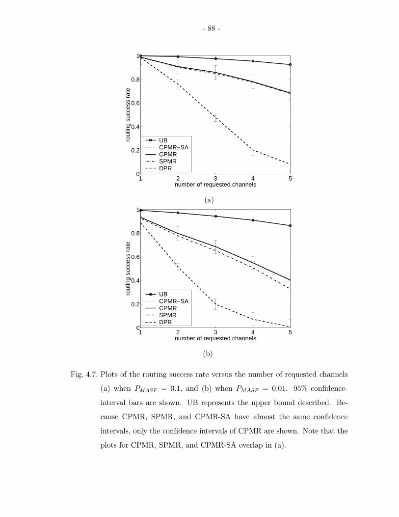
- 88 -
1 2 3 4 50
0.2
0.4
0.6
0.8
1
number of requested channels
rout
ing
succ
ess
rate
UB CPMR−SACPMR SPMR DPR
(a)
1 2 3 4 50
0.2
0.4
0.6
0.8
1
number of requested channels
rout
ing
succ
ess
rate
UB CPMR−SACPMR SPMR DPR
(b)
Fig. 4.7. Plots of the routing success rate versus the number of requested channels
(a) when PMASF = 0.1, and (b) when PMASF = 0.01. 95% confidence-
interval bars are shown. UB represents the upper bound described. Be-
cause CPMR, SPMR, and CPMR-SA have almost the same confidence
intervals, only the confidence intervals of CPMR are shown. Note that the
plots for CPMR, SPMR, and CPMR-SA overlap in (a).
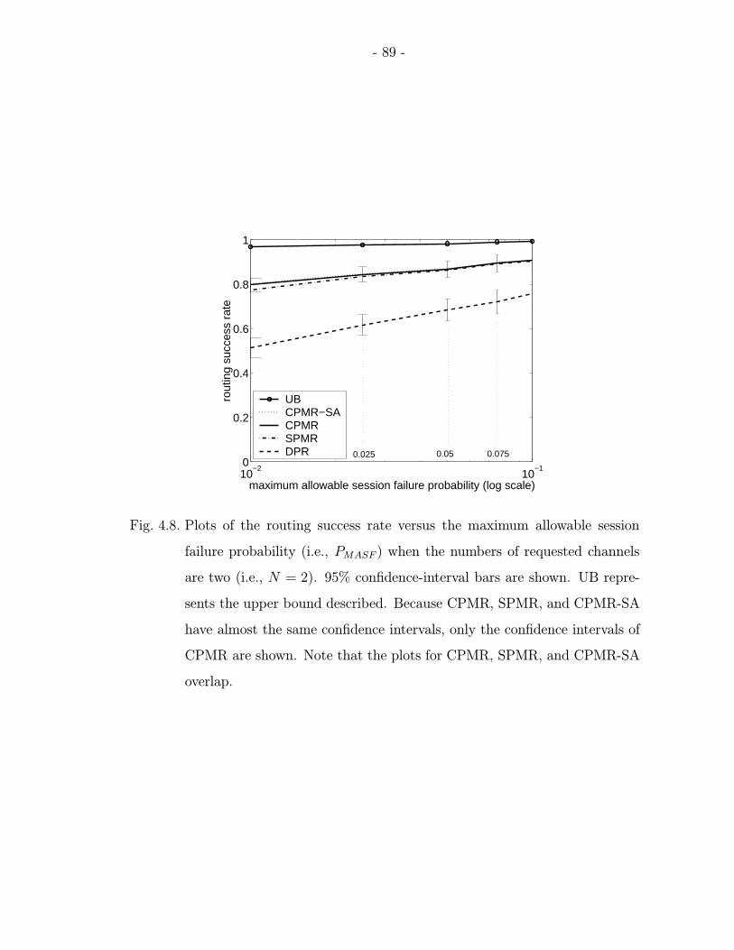
- 89 -
10−2
10−1
0
0.2
0.4
0.6
0.8
1
maximum allowable session failure probability (log scale)
rout
ing
succ
ess
rate
UB CPMR−SACPMR SPMR DPR 0.025 0.05 0.075
Fig. 4.8. Plots of the routing success rate versus the maximum allowable session
failure probability (i.e., PMASF ) when the numbers of requested channels
are two (i.e., N = 2). 95% confidence-interval bars are shown. UB repre-
sents the upper bound described. Because CPMR, SPMR, and CPMR-SA
have almost the same confidence intervals, only the confidence intervals of
CPMR are shown. Note that the plots for CPMR, SPMR, and CPMR-SA
overlap.
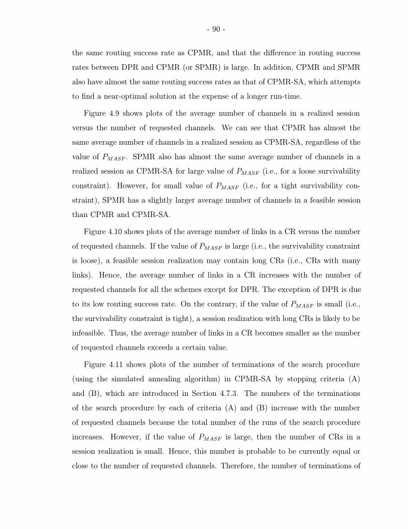
- 90 -
the same routing success rate as CPMR, and that the difference in routing success
rates between DPR and CPMR (or SPMR) is large. In addition, CPMR and SPMR
also have almost the same routing success rates as that of CPMR-SA, which attempts
to find a near-optimal solution at the expense of a longer run-time.
Figure 4.9 shows plots of the average number of channels in a realized session
versus the number of requested channels. We can see that CPMR has almost the
same average number of channels in a realized session as CPMR-SA, regardless of the
value of PMASF . SPMR also has almost the same average number of channels in a
realized session as CPMR-SA for large value of PMASF (i.e., for a loose survivability
constraint). However, for small value of PMASF (i.e., for a tight survivability con-
straint), SPMR has a slightly larger average number of channels in a feasible session
than CPMR and CPMR-SA.
Figure 4.10 shows plots of the average number of links in a CR versus the number
of requested channels. If the value of PMASF is large (i.e., the survivability constraint
is loose), a feasible session realization may contain long CRs (i.e., CRs with many
links). Hence, the average number of links in a CR increases with the number of
requested channels for all the schemes except for DPR. The exception of DPR is due
to its low routing success rate. On the contrary, if the value of PMASF is small (i.e.,
the survivability constraint is tight), a session realization with long CRs is likely to be
infeasible. Thus, the average number of links in a CR becomes smaller as the number
of requested channels exceeds a certain value.
Figure 4.11 shows plots of the number of terminations of the search procedure
(using the simulated annealing algorithm) in CPMR-SA by stopping criteria (A)
and (B), which are introduced in Section 4.7.3. The numbers of the terminations
of the search procedure by each of criteria (A) and (B) increase with the number
of requested channels because the total number of the runs of the search procedure
increases. However, if the value of PMASF is large, then the number of CRs in a
session realization is small. Hence, this number is probable to be currently equal or
close to the number of requested channels. Therefore, the number of terminations of
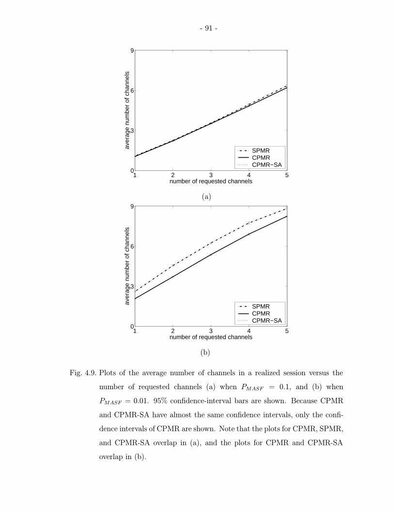
- 91 -
1 2 3 4 50
3
6
9
number of requested channels
aver
age
num
ber
of c
hann
els
SPMR CPMR CPMR−SA
(a)
1 2 3 4 50
3
6
9
number of requested channels
aver
age
num
ber
of c
hann
els
SPMR CPMR CPMR−SA
(b)
Fig. 4.9. Plots of the average number of channels in a realized session versus the
number of requested channels (a) when PMASF = 0.1, and (b) when
PMASF = 0.01. 95% confidence-interval bars are shown. Because CPMR
and CPMR-SA have almost the same confidence intervals, only the confi-
dence intervals of CPMR are shown. Note that the plots for CPMR, SPMR,
and CPMR-SA overlap in (a), and the plots for CPMR and CPMR-SA
overlap in (b).
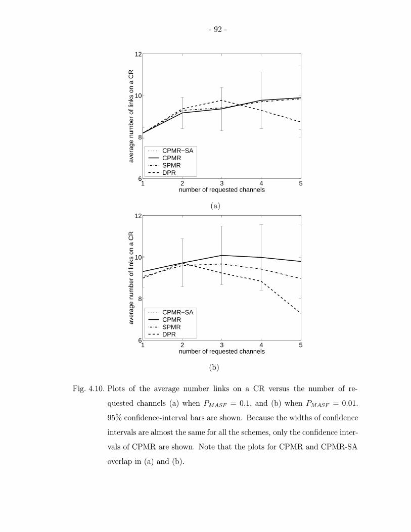
- 92 -
1 2 3 4 56
8
10
12
number of requested channels
aver
age
num
ber
of li
nks
on a
CR
CPMR−SACPMR SPMR DPR
(a)
1 2 3 4 56
8
10
12
number of requested channels
aver
age
num
ber
of li
nks
on a
CR
CPMR−SACPMR SPMR DPR
(b)
Fig. 4.10. Plots of the average number links on a CR versus the number of re-
quested channels (a) when PMASF = 0.1, and (b) when PMASF = 0.01.
95% confidence-interval bars are shown. Because the widths of confidence
intervals are almost the same for all the schemes, only the confidence inter-
vals of CPMR are shown. Note that the plots for CPMR and CPMR-SA
overlap in (a) and (b).
- 93 -
1 2 3 4 50
200
400
600
800
1000
number of requested channels
num
ber
of te
rmin
atio
ns
SC−(A)SC−(B)
(a)
1 2 3 4 50
200
400
600
800
1000
number of requested channels
num
ber
of te
rmin
atio
ns
SC−(A)SC−(B)
(b)
Fig. 4.11. Plots of the number of terminations of the search procedure (using the
simulated annealing algorithm) in CPMR-SA by stopping criteria (A) and
(B), (a) when PMASF = 0.1, and (b) when PMASF = 0.01. SC-(A) and
SC-(B) denote the stopping criteria (A) and (B), respectively.
- 94 -
the search procedure is small because the search procedure (to reduce the number of
CRs in the session realization without violating constraints) is executed no more or
just a few times. The decrease in the number of terminations at the largest number
of requested channels (i.e., 5) in Figure 4.11(b) is due to the low routing success rate.
In our simulation, the run-time of SPMR is approximately 20% of the run-time
of CPMR. The run-time of CPMR-SA is approximately 10 times longer than that of
CPMR. Hence, compared to CPMR-SA, CPMR and SPMR have good performance
in solving the SMR problem, but with much shorter execution time.
4.8 Conclusion
If we do not consider the vulnerability and capacity of each link in survivable
routing for WDM networks, we may waste network resources for unnecessary paths,
or may not provide adequate survivability in practice. To develop survivable rout-
ing schemes without this weakness, we used link failure probabilities to account for
the vulnerability of links in WDM networks, instead of assuming that the maximum
number of link failures is known beforehand. Because our survivable routing prob-
lem is NP-hard, we proposed heuristic schemes, CPMR and SPMR. These schemes
allow link-sharing (i.e., they do not limit routing paths to be disjoint), and thus enjoy
increased routing success rates, compared with schemes without link-sharing. How-
ever, this link-sharing makes routing difficult. Hence, we developed link penalization
methods to deal with this difficulty. These methods make it possible to assign every
link a dynamic value, called a penalty, and update this value to control link-sharing.
CPMR has a longer run-time than SPMR, because of the complicated procedure
to update link penalties. In contrast, SPMR reduces the run-time by the use of a
simple penalization method, but may sacrifice slightly the routing success rate and
the average number of channels in a feasible session. We compared our schemes
with DPR (which searches for disjoint paths) and with CPMR-SA (which uses a
simulated-annealing method to search for a near-optimal solution at the expense of
- 95 -
a longer run-time). Via simulation, we showed that our schemes have higher routing
success rates than DPR, and achieve (with shorter execution times) almost the same
routing success rate and average number of channels in a realized session as CPMR-
SA. Future work could involve examining how these schemes may be adapted to the
situations where there are multiple pairs of source and destination nodes.
- 96 -
5. SUMMARY AND DIRECTIONS FOR FUTURE
RESEARCH
In this thesis, we dealt with two routing problems. The first problem, called the
multiconstraint QoS routing problem, is to find a single path that satisfies multiple
QoS (quality of service) constraints. We develop two routing schemes, called MPLMR
and SPMP, for this problem. The second problem, which we call the survivable
multipath routing problem, is to find a minimum number of paths that can collectively
satisfy the constraints on channel demand, capacity, and survivability, between a given
pair of source and destination nodes in a WDM (wavelength division multiplexing)
network. We also develop two schemes, CPMR and SPMR, for the second problem.
MPLMR uses an extended shortest-path algorithm based on the notion of the non-
linear path length, with the assumption that detailed routing information is provided
by a link-state protocol. Like previous schemes using extended shortest-path algo-
rithms for polynomial complexity, MPLMR stores a limited number of prepaths, and
extends them toward the destination node. However, unlike the previous schemes,
MPLMR uses an efficient “look-ahead” method to predict the nonlinear path length of
the full path to which each prepath is extended, and selects and stores the prepaths
that have higher likelihood than other prepaths to be extended to feasible paths.
MPLMR has a significantly low EDR with even smaller execution time than the com-
peting schemes in the literature. Hence, MPLMR provides a promising solution for
multiconstraint QoS routing when detailed routing information is provided by a link-
state protocol. Future research related to MPLMR may include the following topics:
(1) estimation of the optimal value of k (i.e., the maximum number of prepaths to
be stored for each node), (2) improvement of the look-ahead method using statistical
data about link values (e.g., correlation between QoS attributes), and (3) analysis
- 97 -
of the sensitivity of MPLMR to inaccurate routing information and development of
enhanced routing schemes robust to dynamic routing environments.
SPMP is also a multiconstraint QoS routing scheme based on the notion of the
nonlinear path length. However, SPMP assumes that routing information is pro-
vided by a distance-vector protocol to reduce the signaling overhead in both the
information-advertisement process and the path-search process. Moreover, SPMP
takes a sequential path-search approach to minimize the number of the nodes unnec-
essarily affected by the path-search process. Because of the sequential path-search
approach, SPMP has exponential worst-case time complexity. However, by the use of
an efficient path-search order and the control of the crankback degree, SPMP shows
low EDR while keeping average-case time complexity low. Hence, SPMP can be a
useful tool for multiconstraint QoS routing when the signaling overhead is a con-
cern (e.g., wireless ad hoc networks). SPMP can be extended to the corresponding
parallel path-search scheme for the reduction of path-search time. It may be valu-
able to compare quantitatively the advantages and disadvantages of both SPMP and
the corresponding parallel search scheme. In addition, the development of an effi-
cient multiconstraint QoS routing scheme with no information advertisement may
also be a valuable research topic for the elimination of the signaling overhead in the
information-advertisement process.
Both CPMR and SPMR are survivable multipath routing schemes to find a set of
routing paths that accommodate the minimum number of channels without violating
the constraints. Implicitly or explicitly, most previous survivable routing schemes for
WDM networks assume that the maximum number of simultaneous link failures is
known. However, CPMR and SPMR take an alternative approach by using failure
probability for more general assumption on survivability. These schemes do not limit
routing paths to be disjoint to increase routing success rates. To control the difficulty
caused by link-sharing, we develop link penalization methods for CPMR and SPMR.
We compare these schemes with DPR (which searches for disjoint paths) and with
CPMR-SA (which uses a simulated-annealing method to search for a near-optimal
- 98 -
solution at the expense of a longer run-time). Via simulation, we show that CPMR
and SPMR have higher routing success rates than DPR, and achieve (with shorter
execution times) almost the same routing success rate and average number of channels
in a realized session as CPMR-SA. Future work could involve examining how these
schemes may be adapted to situations where there are multiple pairs of source and
destination nodes.

LIST OF REFERENCES
- 99 -
LIST OF REFERENCES
[AhM93] R. K. Ahuja, T. L. Magnanti, and J. B. Orlin, Network Flows, PrenticeHall, Upper Saddle River, NJ, 1993.
[Ban99] A. Banerjea, “Fault recovery for guaranteed performance communicationsconnections,” IEEE/ACM Transactions on Networking, Vol. 7, No. 5, Oct.1999, pp. 653–668.
[CaP98] B. V. Caenegem, W. V. Parys, F. D. Turck, and P. M. Demeester, “Dimen-sioning of survivable WDM networks,” IEEE Journal on Selected Areas inCommunications, Vol. 16, No. 7, Sep. 1998, pp. 1146–1157.
[ChC00] C. Jin, Q. Chen, and S. Jamin, “Inet: Internet topology generator,” De-partment of Electrical Engineering and Computer Science, University ofMichigan, 2000, http://topology.eecs.umich.edu/inet/.
[ChC95] R.-S. Chen, D.-J. Chen, and Y. S. Yeh, “Reliability optimization of dis-tributed computing systems subject to capacity constraints,” Computersand Mathematics with Applications, Vol. 29, No. 4, Feb. 1995, pp. 93–99.
[ChC99] D. J. Chen and P. Y. Chang, “An efficient multipath routing for distributedcomputing systems with data replication,” Information Sciences, Vol. 120,No. 1-4, Nov. 1999, pp. 143–157.
[ChH01] B.-J. Chang and R.-H. Hwang, “Efficient hierarchical QoS routing in ATMnetworks,” Computer Communications, Vol. 24, No. 15-16, Oct. 2001,pp. 1648–1660.
[ChN98a] S. Chen and K. Nahrstedt, “On finding multi-constrained paths,” IEEEInternational Conference on Communications (ICC), Vol. 2, June 1998,pp. 874–879.
[ChN98b] S. Chen and K. Nahrstedt, “Distributed quality-of-service routing in high-speed networks based on selective probing,” IEEE Conference on LocalComputer Networks (LCN), Oct. 1998, pp. 80–89.
[ChN99] S. Chen and K. Nahrstedt, “Distributed quality-of-service routing in ad-hocnetworks,” IEEE Journal on Selected Areas in Communications, Vol. 17,No. 8, Aug. 1999, pp. 1488–1505.
[CiR97] I. Cidon, R. Rom, and Y. Shavitt, “Multi-path routing combined withresource reservation,” IEEE INFOCOM, Vol. 1, Apr. 1997, pp. 92–100.
[CoL90] T. H. Cormen, C. E. Leiserson, and R. L. Rivest, Introduction to Algorithms,2nd Edition, MIT Press, New York, NY, 1990.
- 100 -
[CrB98] O. Crochat and J.-Y. L. Boudec, “Design protection for WDM optical net-works,” IEEE Journal on Selected Areas in Communications, Vol. 16, No. 7,Sep. 1998, pp. 1158–1165.
[CuX03] Y. Cui, K. Xu, and J. Wu, “Precomputation for multi-constrained QoS rout-ing in high-speed networks,” IEEE INFOCOM, Vol. 2, Apr. 2003, pp. 1414–1424.
[DoD99] B. T. Doshi, S. Dravida, P. Harshavardhana, O. Hauser, and Y. Wang, “Op-tical network design and restoration,” Bell Labs Technical Journal, Vol. 4,No. 1, Jan.-Mar. 1999, pp. 58–84.
[FeM02] G. Feng, K. Makki, N. Pissinou, and C. Douligeris, “Heuristic and exactalgorithms for QoS routing with multiple constraints,” IEICE Transactionson Communications, Vol. E85-B, No. 12, Dec. 2002, pp. 2838–2850.
[FoS99] N. Ghani and S. Dixit, “Channel provisioning for higher-layer protocolsin WDM networks,” International Workshop on Randomization and Ap-proximation Techniques in Computer Science, and International Workshopon Approximation Algorithms for Combinatorial Optimization Problems(RANDOM-APPROX), Aug. 1999, pp. 156–167.
[Fra90] A. Frank, “Packing paths, circuits, and cuts - A survey,” in Paths, flows,and VLSI-layout, B. Korte, L. Lovasz, H. J. Promel, and A. Schrijver, eds.,Springer-Verlag, Berlin, Germany, 1990, pp. 47–100.
[Fuk90] K. Fukunaga, Introduction to Statistical Pattern Recognition, 2nd Edition,Academic Press, Boston, MA, 1990.
[GhD99] N. Ghani and S. Dixit, “Channel provisioning for higher-layer protocols inWDM networks,” All Optical Networking 1999: Architecture, Control, andManagement Issues, Sep. 1999, pp. 22–32.
[GhS01] D. Ghosh, V. Sarangan, and R. Acharya, “Quality-of-service routing in IPnetworks,” IEEE Transactions on Multimedia, Vol. 3, No. 2, June 2001,pp. 200–208.
[GuO97] R. Guerin and A. Orda, “QoS-based routing in networks with inaccurateinformation: Theory and algorithms,” IEEE INFOCOM, Vol. 1, Apr. 1997,pp. 75–83.
[HaL02] J. Harmatos and P. Laborczi, “Dynamic routing and wavelength assignmentin survivable WDM networks,” Photonic Network Communications, Vol. 4,No. 3-4, Jul.-Dec. 2002, pp. 357–376.
[Haj88] B. Hajek, “Cooling schedules for optimal annealing,” Mathematics of Op-erations Research, Vol. 13, No. 2, May 1988, pp. 311–329.
[Has92] R. Hassin, “Approximation schemes for the restricted shortest path prob-lem,” Mathematics of Operations Research, Vol. 17, No. 1, Feb. 1992,pp. 36–42.
[Hen85] M. I. Henig, “The shortest path problem with two objective functions,” Eu-ropean Journal of Operational Research, Vol. 25, No. 2, May 1985, pp. 281–291.
- 101 -
[HsH01] P.-H. Hsiao, A. Hwang, H. T. Kung, and D. Vlah, “Load-balancing routingfor wireless access networks,” IEEE INFOCOM, Vol. 2, Apr. 2001, pp. 986–995.
[HwA01] H. Hwang, S. Ahn, Y. Yoo, and C. S. Kim, “Multiple shared backup cyclesfor survivable optical mesh networks,” IEEE International Conference onComputer Communications and Networks, Oct. 2001, pp. 284–289.
[Jaf84] J. M. Jaffe, “Algorithms for finding paths with multiple constraints,” Net-works, Vol. 14, No. 1, Spring 1984, pp. 95–116.
[KoK01] T. Korkmaz and M. Krunz, “Multi-constrained optimal path selection,”IEEE INFOCOM, Vol. 2, Apr. 2001, pp. 834–843.
[KoK99] T. Korkmaz and M. Krunz, “A randomized algorithm for finding a pathsubject to multiple QoS constraints,” IEEE Globecom, Dec. 1999, pp. 1694–1698.
[Kot96] G. Kotelly, “Worldwide fiber-optic markets to expand unabated,” Light-wave, Vol. 13, No. 13, Dec. 1996, pp. 6–8.
[KuM02] F. Kuipers, P. V. Mieghem, T. Korkmaz, and M. Krunz, “An overview ofconstraint-based path selection algorithms for QoS routing,” IEEE Com-munications Magazine, Vol. 40, No. 12, Dec. 2002, pp. 50–55.
[Kya98] K. Kyandoghere, “Survivability performance analysis of rerouting strategiesin an ATM/VP DCS survivable mesh network,” Computer CommunicationReview, Vol. 28, No. 5, Oct. 1998, pp. 22–49.
[LiR01] G. Liu and K. G. Ramakrishnan, “A* Prune: An algorithm for finding kshortest paths subject to multiple constraints,” IEEE INFOCOM, Vol. 2,Apr. 2001, pp. 743–749.
[LoF01] W. Lou and Y. Fang, “A multipath routing approach for secure data deliv-ery,” Military Communication Conference (MILCOM), Vol. 2, Oct. 2001,pp. 1467–1473.
[MaS95] G. S. Malkin and M. E. Steenstrup, “Distance-vector routing,” in Routing inCommunications Networks, M. E. Steenstrup, ed., Prentice Hall, EnglewoodCliffs, NJ, 1995, pp. 83–98.
[MaS97] Q. Ma and P. Steenkiste, “Quality-of-service routing for traffic with per-formance guarantees,” IFIP International Workshop on Quality of Service(IWQoS), May 1997, pp. 115–126.
[MiL02] J. Miller, “RandGen: A program for generating random numbers,” Depart-ment of Psychology, University of Otago, New Zealand, Version 2.0, Sep.2002, http://www.winsite.com.
[MiN01] P. V. Mieghem, H. D. Neve, and F. Kuipers, “Hop-by-hop quality of servicerouting,” Computer Networks, Vol. 37, No. 3-4, Nov. 2001, pp. 407–423.
[MoN02] E. Modiano and A. Narula-Tam, “Survivable lightpath routing: A newapproach to the design of WDM-based networks,” IEEE Journal on SelectedAreas in Communications, Vol. 20, No. 4, May 2002, pp. 800–809.
- 102 -
[Moy95] J. Moy, “Link-state routing,” in Routing in Communications Networks,M. E. Steenstrup, ed., Prentice Hall, Englewood Cliffs, NJ, 1995, pp. 135–157.
[MuG96] S. Murthy and J. J. Garcia-Luna-Aceves, “Congestion-oriented shortestmultipath routing,” IEEE INFOCOM, Vol. 3, Mar. 1996, pp. 1028–1036.
[NeM00] H. D. Neve and P. V. Mieghem, “TAMCRA: A tunable accuracy multipleconstraints routing algorithm,” Computer Communications, Vol. 23, No. 7,Mar. 2000, pp. 667–679.
[PoC97] C. Pornavalai, G. Chakraborty, and N. Shiratori, “A new distributed QoSrouting algorithm for supporting real-time communication in high-speednetworks,” IEICE Transactions on Communications, Vol. E80-B, No. 10,Oct. 1997, pp. 1493–1501.
[RaM99] S. Ramamuthy and B. Mukherjee, “Survivable WDM mesh networks, partI - Protection,” IEEE INFOCOM, Vol. 2, Mar. 1999, pp. 744–751.
[ReS00] D. S. Reeves and H. F. Salama, “A distributed algorithm for delay-constrained unicast routing,” IEEE/ACM Transactions on Networking,Vol. 8, No. 2, Apr. 2000, pp. 239–250.
[RoB02] A. Roy, N. Banerjee, and S. K. Das, “An efficient multi-objective QoS-routing algorithm for wireless multicasting,” Vehicular Technology Confer-ence (VTC), Vol. 3, May 2002, pp. 1160–1164.
[RoB97] G. N. Rouskas and I. Baldine, “Multicast routing with end-to-end delayand delay variation constraints,” IEEE Journal on Selected Areas in Com-munications, Vol. 15, No. 3, Apr. 1997, pp. 346–356.
[RoS91] J. B. Rosen, S. Z. Sun, and G.-L. Xue, “Algorithms for the quickest pathproblem and the enumeration of quickest paths,” Computers and OperationsResearch, Vol. 18, No. 6, 1991, pp. 579–584.
[SeH02] A. Sen, B. Hao, B. H. Shen, and G. Lin, “Survivable routing in WDMnetworks - Logical ring in arbitrary physical topology,” IEEE InternationalConference on Communications (ICC), Vol. 5, Apr.-May 2002, pp. 2771–2775.
[ShC02] D. Shin, E. K. P. Chong, and H. J. Siegel, “A multiconstraint QoS routingscheme using a modified Dijkstra’s algorithm,” Networks 2002 (joint confer-ence of IEEE International Conference Wireless LANs and Home Networksand IEEE International Conference on Networking), Aug. 2002, pp. 65–76.
[ShC95] K. G. Shin and C. C. Chou, “A distributed route selection for establishingreal-time channels,” IFIP International Conference on High PerformanceNetworking, Sep. 1995, pp. 319–329.
[SiG94] B. Singh and S. K. Ghosh, “Network reliability evaluation by decomposi-tion,” Microelectronics Reliability, Vol. 34, No. 5, May 1994, pp. 925–927.
[SoP00] J. Song, H. K. Pung, and L. Jacob, “A multi-constrained distributed qosrouting algorithm,” International Conference on Networks (ICON), Sep.2000, pp. 165–171.
- 103 -
[SrR02] N. Sreenath, P. P. Rao, G. Mohan, and C. S. R. Murthy, “Design of surviv-able WDM networks for carrying ATM traffic,” Computer Communications,Vol. 25, No. 5, Mar. 2002, pp. 485–500.
[SrS02] M. Sridharan, M. V. Salapaka, and A. K. Somani, “A practical approachto operating survivable WDM networks,” IEEE Journal on Selected Areasin Communications, Vol. 20, No. 1, Jan. 2002, pp. 34–46.
[WaC96] Z. Wang and J. Crowcroft, “Quality-of-service routing for supporting multi-media applications,” IEEE Journal on Selected Areas in Communications,Vol. 14, No. 7, Sep. 1996, pp. 1228–1234.
[WaV00] J. Walrand and P. Varaiya, High-Performance Communication Networks,2nd Edition, Morgan Kaufmann Publishers, San Francisco, CA, 2000.
[Wan99] Z. Wang, “On the complexity of quality of service routing,” InformationProcessing Letters, Vol. 69, No. 3, Feb. 1999, pp. 111–114.
[Wax88] B. M. Waxman, “Routing of multipoint connections,” IEEE Journal onSelected Areas in Communications, Vol. 6, No. 9, Dec. 1988, pp. 1617–1622.
[WuH00] J.-J. Wu, R.-H. Hwang, and H.-I. Lu, “Multicast routing with multiple qosconstraints in atm networks,” Information Sciences, Vol. 124, No. 1-4, May2000, pp. 29–57.
[Xue00] G. Xue, “Optimal multi-path end-to-end data transmission in networks,”IEEE Symposium on Computer and Communications (ISCC), July 2000,pp. 581–586.
[Yua02] X. Yuan, “Heuristic algorithms for multiconstrained quality-of-service rout-ing,” IEEE/ACM Transactions on Networking, Vol. 10, No. 2, Apr. 2002,pp. 244–256.
[ZaO03] H. Zang, C. Ou, and B. Mukherjee, “Path-protection routing and wave-length assignment (RWA) in WDM networks under duct-layer constraints,”IEEE/ACM Transactions on Networking, Vol. 11, No. 2, Apr. 2003,pp. 248–258.
[ZhZ02] L. Zhang, Z. Zhao, Y. Shu, L. Wang, and O. W. W. Yang, “Load balanc-ing of multipath source routing in ad hoc networks,” IEEE InternationalConference on Communications (ICC), Vol. 5, Apr. 2002, pp. 3197–3201.

APPENDIX
- 104 -
APPENDIX A
COMPUTATION OF THE PROBABILITY IN (4.2)
If we can compute P (x(F )1 , . . . , x
(F )k , x
(W )k+1, . . . , x
(W )L ), then we can compute the
probability of (4.2) by applying the same computation to all the terms in the equation.
By Bayes’ rule,
P (x(F )1 , . . . , x
(F )k , x
(W )k+1, . . . , x
(W )L )
= P (x(F )1 , . . . , x
(F )k | x
(W )k+1, . . . , x
(W )L ) · P (x
(W )k+1, . . . , x
(W )L ).
The computation of P (x(W )k+1, . . . , x
(W )L ) is straightforward, as follows. Let Ew be the
set of links on CRs xk+1, . . . , xL, and let Pf (uv) be the failure probability of link
uv ∈ Ew. If CRs xk+1, . . . , xL work, all the links on these CRs must be working.
Hence,
P (x(W )k+1, . . . , x
(W )L ) =
∏uv∈Ew
[ 1− Pf(uv) ]. (A.1)
Next, we consider the computation of P (x(F )1 , . . . , x
(F )k | x
(W )k+1, . . . , x
(W )L ). Let Ek
be the set of the links on CRs x1, . . . , xk. We do not need to consider the failure
probabilities of the links on CRs xk+1, . . . , xL, because these links are assumed to be
working. Thus, we consider only the links in Ek −Ew. Let h be the number of these
links. We can compute P (x(F )1 , . . . , x
(F )k | x
(W )k+1, . . . , x
(W )L ) by investigating the 2h cases
where each link works or fails, and summing up all the probabilities of the cases for
which CRs x1, . . . , xk fail. For this computation, let Hh = {1, . . . , h}, Bi the set of
the CRs containing link li, and Pf(li) the failure probability of link li for i = 1, . . . , h.
Then,
P (x(F )1 , . . . , x
(F )k | x
(W )k+1, . . . , x
(W )L )
=h∑i=1
∑{j1,...,ji}⊂Hh s. t.
Bj1∪...∪Bji
={x1,...,xk},
{ji+1,...,jh}=Hh−{j1,...,ji}
Pf(lj1) · · ·Pf(lji) · [1− Pf(lji+1)] · · · [1− Pf(ljh)]. (A.2)

- 105 -
The computation of (A.2) has the exponential complexity of O(2h), and may require
long computation time.
If k is sufficiently small compared to h (as described below), then we can reduce
the computation time of (A.2) as follows. First, we group the h links into 2k groups
according to their associated CRs among x1, . . . , xk, such that all the links in each
group are on the same subset of CRs, and not on any other CRs (the total number
of subsets of k CRs is 2k). In general, some of these groups are empty. If we use
link penalization, then typically the majority of the groups are empty because link-
sharing is discouraged. Note that if any of the links in a group fails, then all of the
CRs associated with the group fail. It is easy to compute the probability that any
of the links in each group fails, which we call the group failure probability. We can
compute the group failure probability of group gi, denoted by Pf (gi), as in (A.1).
That is,
Pf(gi) = 1−∏uv∈gi
[ 1− Pf(uv) ].
Let the number of the groups containing at least one link be r. The computation of
the group failure probabilities for all the groups takes O(h) time. Using the group
failure probabilities (rather than the failure probabilities of links l1, . . . , lh), we can
compute P (x(F )1 , . . . , x
(F )k | x
(W )k+1, . . . , x
(W )L ) as follows. Let Hr = {1, . . . , r}, and Ci be
the set of the CRs associated with group gi for i = 1, . . . , r. Then,
P (x(F )1 , . . . , x
(F )k | x
(W )k+1, . . . , x
(W )L )
=r∑i=1
∑{j1,...,ji}⊂Hr s. t.
Cj1∪...∪Cji
={x1,...,xk},
{ji+1,...,jr}=Hr−{j1,...,ji}
Pf(gj1) · · ·Pf (gji) · [1− Pf(gji+1)] · · · [1− Pf(gjr)]. (A.3)
Hence, the computation of (A.3) has the complexity of O(h+ 2r), which, like (A.2),
is also exponential. However, if r < h (i.e., the number of groups is smaller than the
number of links), then the computation time is smaller than that of (A.2).
- 106 -
APPENDIX B
COMPUTATION OF THE PENALTY IN (4.8)
By the method explained in Appendix 1, we can compute P (X, k, b). Using the
notation used in (4.2), we can represent P (X, k, b | uv fails) as follows:
P (X, k, b | uv fails) =∑
{j1,...,jb}⊂Hk,{jb+1,...,jk}=Hk−{j1,...,jb}
P (x(F )j1, . . . , x
(F )jb, x
(W )jb+1
, . . . , x(W )jk| uv fails).
(B.1)
Hence, if we can compute P ∗ = P (x(F )1 , . . . , x
(F )b , x
(W )b+1 , . . . , x
(W )k | uv fails), then we
can compute the link penalty of (4.8) by applying the same computation to all the
terms in (B.1).
If link uv is not on any of CRs x1, . . . , xk, then P ∗ =
P (x(F )1 , . . . , x
(F )b , x
(W )b+1 , . . . , x
(W )k ). Obviously, P ∗ is zero if link uv is on any of
the working CRs xb+1, . . . , xk. Hence, it remains to consider the case where link
uv is on some of CRs x1, . . . , xb but not on any of CRs xb+1, . . . , xk. Without loss
of generality, we assume that link uv is only on CRs x1, . . . , xa (a ≤ b). Then,
P ∗ = P (x(F )a+1, . . . , x
(F )b , x
(W )b+1 , . . . , x
(W )k ). By the method explained in Appendix 1, we
can also compute this P ∗.

VITA

- 107 -
VITA
Dong-won Shin was born in Seoul, Korea, on November 22, 1968. He received
B.S. and M.S. degrees from the Electronic Engineering Department of Seoul National
University in 1991 and 1993, respectively. In March 1993, he joined KT (formerly
known as Korea Telecom), and worked for the company about five and half years as
a member of the technical staff. He participated in the IMT-2000 standardization
activities of ITU (International Telecommunication Union) as a delegate from KT
between March 1996 and July 1998. Since then he has been working towards his Ph.D.
degree in the School of Electrical and Computer Engineering, Purdue University. His
current research interests include multiconstraint and/or multipath routing. After
graduation in August 2003, he will rejoin KT.


