
Ch5 Data Mining Classification: Alternative Techniques

Rule-Based Classifier
• Classify records by using a collection of “if…then…” rules
• Rule: (Condition) y– where
• Condition is a conjunctions of attributes
• y is the class label
– LHS: rule antecedent or condition
– RHS: rule consequent
– Examples of classification rules:• (Blood Type=Warm) (Lay Eggs=Yes) Birds
• (Taxable Income < 50K) (Refund=Yes) Evade=No

Rule-based Classifier (Example)Name Blood Type Give Birth Can Fly Live in Water Class
human warm yes no no mammalspython cold no no no reptilessalmon cold no no yes fisheswhale warm yes no yes mammalsfrog cold no no sometimes amphibianskomodo cold no no no reptilesbat warm yes yes no mammalspigeon warm no yes no birdscat warm yes no no mammalsleopard shark cold yes no yes fishesturtle cold no no sometimes reptilespenguin warm no no sometimes birdsporcupine warm yes no no mammalseel cold no no yes fishessalamander cold no no sometimes amphibiansgila monster cold no no no reptilesplatypus warm no no no mammalsowl warm no yes no birdsdolphin warm yes no yes mammalseagle warm no yes no birds
R1: (Give Birth = no) (Can Fly = yes) Birds
R2: (Give Birth = no) (Live in Water = yes) Fishes
R3: (Give Birth = yes) (Blood Type = warm) Mammals
R4: (Give Birth = no) (Can Fly = no) Reptiles
R5: (Live in Water = sometimes) Amphibians

Application of Rule-Based Classifier
Name Blood Type Give Birth Can Fly Live in Water Class
hawk warm no yes no ?grizzly bear warm yes no no ?
• A rule r covers an instance x if the attributes of the instance satisfy the condition of the rule
R1: (Give Birth = no) (Can Fly = yes) Birds
R2: (Give Birth = no) (Live in Water = yes) Fishes
R3: (Give Birth = yes) (Blood Type = warm) Mammals
R4: (Give Birth = no) (Can Fly = no) Reptiles
R5: (Live in Water = sometimes) Amphibians
The rule R1 covers a hawk => Bird
The rule R3 covers the grizzly bear => Mammal

Rule Coverage and Accuracy• Coverage of a rule:
– Fraction of records that satisfy the antecedent of a rule
• Accuracy of a rule:
– Fraction of records that satisfy both the antecedent and consequent of a rule
Tid Refund Marital Status
Taxable Income Class
1 Yes Single 125K No
2 No Married 100K No
3 No Single 70K No
4 Yes Married 120K No
5 No Divorced 95K Yes
6 No Married 60K No
7 Yes Divorced 220K No
8 No Single 85K Yes
9 No Married 75K No
10 No Single 90K Yes 10
(Status=Single) No
Coverage = 40%, Accuracy = 50%

How does Rule-based Classifier Work?
Name Blood Type Give Birth Can Fly Live in Water Class
lemur warm yes no no ?turtle cold no no sometimes ?dogfish shark cold yes no yes ?
R1: (Give Birth = no) (Can Fly = yes) Birds
R2: (Give Birth = no) (Live in Water = yes) Fishes
R3: (Give Birth = yes) (Blood Type = warm) Mammals
R4: (Give Birth = no) (Can Fly = no) Reptiles
R5: (Live in Water = sometimes) Amphibians
A lemur triggers rule R3, so it is classified as a mammal
A turtle triggers both R4 and R5
A dogfish shark triggers none of the rules
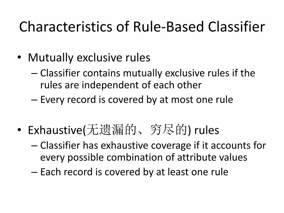
Characteristics of Rule-Based Classifier
• Mutually exclusive rules– Classifier contains mutually exclusive rules if the
rules are independent of each other
– Every record is covered by at most one rule
• Exhaustive(无遗漏的、穷尽的) rules– Classifier has exhaustive coverage if it accounts for
every possible combination of attribute values
– Each record is covered by at least one rule

From Decision Trees To Rules
YESYESNONO
NONO
NONO
Yes No
{Married}{Single,
Divorced}
< 80K > 80K
Taxable
Income
Marital
Status
Refund
Classification Rules
(Refund=Yes) ==> No
(Refund=No, Marital Status={Single,Divorced},
Taxable Income<80K) ==> No
(Refund=No, Marital Status={Single,Divorced},
Taxable Income>80K) ==> Yes
(Refund=No, Marital Status={Married}) ==> No
Rules are mutually exclusive and exhaustive
Rule set contains as much information as the
tree
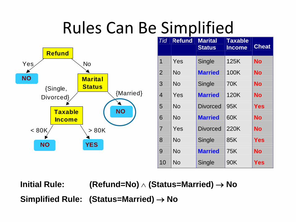
Rules Can Be Simplified
YESYESNONO
NONO
NONO
Yes No
{Married}{Single,
Divorced}
< 80K > 80K
Taxable
Income
Marital
Status
Refund
Tid Refund Marital Status
Taxable Income Cheat
1 Yes Single 125K No
2 No Married 100K No
3 No Single 70K No
4 Yes Married 120K No
5 No Divorced 95K Yes
6 No Married 60K No
7 Yes Divorced 220K No
8 No Single 85K Yes
9 No Married 75K No
10 No Single 90K Yes 10
Initial Rule: (Refund=No) (Status=Married) No
Simplified Rule: (Status=Married) No

Effect of Rule Simplification• Rules are no longer mutually exclusive
– A record may trigger more than one rule
– Solution?• Ordered rule set(有序规则)
• Unordered rule set(无序规则)
– 采用投票策略,把每条被触发的后件看作是对相应类的一次投票,然后计票确定测试记录的类标号;
– 在某些情况下,投票可以用规则的准确率加权;
– 利:不易受由于选择不当的规则而产生错误的影响;不必维护规则的顺序,建立模型的开销也相对较小;
– 弊:测试记录的属性要与规则集中的每一条规则的前件作比较,所以对测试记录进行分类是一件很繁重的任务。
• Rules are no longer exhaustive– A record may not trigger any rules
– Solution?• Use a default class {} y

Ordered Rule Set
Name Blood Type Give Birth Can Fly Live in Water Class
turtle cold no no sometimes ?
• Rules are ranked in descending order according to their priority(按优先级降序排列)– 优先级的定义有多种方法:基于准确率、覆盖率、总描述长度或规则的产生顺序
– 有序的规则集也成为决策表( decision list)
• When a test record is presented to the classifier
– It is assigned to the class label of the highest ranked rule(排序最高的规则)it has triggered
– If none of the rules fired, it is assigned to the default class
R1: (Give Birth = no) (Can Fly = yes) Birds
R2: (Give Birth = no) (Live in Water = yes) Fishes
R3: (Give Birth = yes) (Blood Type = warm) Mammals
R4: (Give Birth = no) (Can Fly = no) Reptiles
R5: (Live in Water = sometimes) Amphibians

Rule Ordering Schemes
Rule-based Ordering
(Refund=Yes) ==> No
(Refund=No, Marital Status={Single,Divorced},
Taxable Income<80K) ==> No
(Refund=No, Marital Status={Single,Divorced},
Taxable Income>80K) ==> Yes
(Refund=No, Marital Status={Married}) ==> No
Class-based Ordering
(Refund=Yes) ==> No
(Refund=No, Marital Status={Single,Divorced},
Taxable Income<80K) ==> No
(Refund=No, Marital Status={Married}) ==> No
(Refund=No, Marital Status={Single,Divorced},
Taxable Income>80K) ==> Yes
• Rule-based ordering– Individual rules are ranked based on their quality:依据规则质量的某种度量对规则
排序,该方案确保每一个测试记录都是由覆盖它的“最好的”规则来分类
– 该方案的潜在缺点是排在越低的规则越难解释,因为每条规则都假设所有排在它前面的规则不成立
• Class-based ordering– Rules that belong to the same class appear together
– 质量较差的规则可能因为某个类的优先级较高排在前面而被触发,从而导致高质量规则被忽略。

Building Classification Rules
• Direct Method: • Extract rules directly from data
• e.g.: RIPPER, CN2, Holte’s 1R
• Indirect Method:• Extract rules from other classification models (e.g.
decision trees, neural networks, etc).
• e.g: C4.5rules

Direct Method: Sequential Covering1. Start from an empty rule
2. Grow a rule using the Learn-One-Rule function
3. Remove training records covered by the rule
4. Repeat Step (2) and (3) until stopping criterion is met
1. 令E是训练记录,A是属性-值对的集合{(Aj, vj)}
2. 令Y0是类的有序集{y1, y1, …, yk}
3. 令R={}是初始规则列表
4. for 每个类y Y0 -{yk} do
5. while 终止条件不满足 do
6. r Learn-one-rule(E, A, y)
7. 从E中删除被r覆盖的训练记录
8. 追加r到规则列表尾部:R R v r
9. end while
10. end for
11. 把默认规则{ } yk插入到规则列表R尾部

Example of Sequential Covering
(i) Original Data (ii) Step 1

Example of Sequential Covering…
(iii) Step 2
R1
(iv) Step 3
R1
R2

Aspects of Sequential Covering
• Rule Growing
• Instance Elimination
• Rule Evaluation
• Stopping Criterion
• Rule Pruning

Rule Growing
• Two common strategies
• 先建立一个初始规则r: { } y (质量很差, 覆盖所有样本)
• 加入新的合取项提高规则的质量。探查所有可能的候选,并贪心地选择下一个合取项。
• 继续该过程,直至满足终止条件为止
Status =
Single
Status =
DivorcedStatus =
Married
Income
> 80K...
Yes: 3
No: 4{ }
Yes: 0
No: 3
Refund=
No
Yes: 3
No: 4
Yes: 2
No: 1
Yes: 1
No: 0
Yes: 3
No: 1
(a) General-to-specific
Refund=No,
Status=Single,
Income=85K
(Class=Yes)
Refund=No,
Status=Single,
Income=90K
(Class=Yes)
Refund=No,
Status = Single
(Class = Yes)
(b) Specific-to-general• 可以随机选择一个正例作为规则增长的初始
种子
• 求精步,通过删除规则的一个合取项,使其覆盖更多的正例来泛化规则。
• 继续该过程,直至满足终止条件为止
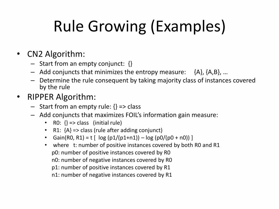
Rule Growing (Examples)
• CN2 Algorithm:– Start from an empty conjunct: {}– Add conjuncts that minimizes the entropy measure: {A}, {A,B}, …– Determine the rule consequent by taking majority class of instances covered
by the rule
• RIPPER Algorithm:– Start from an empty rule: {} => class– Add conjuncts that maximizes FOIL’s information gain measure:
• R0: {} => class (initial rule)• R1: {A} => class (rule after adding conjunct)• Gain(R0, R1) = t [ log (p1/(p1+n1)) – log (p0/(p0 + n0)) ]• where t: number of positive instances covered by both R0 and R1
p0: number of positive instances covered by R0n0: number of negative instances covered by R0p1: number of positive instances covered by R1n1: number of negative instances covered by R1

Instance Elimination
• Why do we need to eliminate instances?– Otherwise, the next rule is
identical to previous rule
• Why do we remove positive instances?– Ensure that the next rule is
different
• Why do we remove negative instances?– Prevent underestimating
accuracy of rule
– Compare rules R2 and R3 in the diagram
class = +
class = -
+
+ +
++
++
+
++
+
+
+
+
+
+
++
+
+
-
-
--
- --
--
- -
-
-
-
-
--
-
-
-
-
+
+
++
+
+
+
R1
R3 R2
+
+

Rule Evaluation
• Statistical test-For example, compute the following likelihood ratio statistic:
-Where k is the number of classes, is the observed frequency of class iexamples that are covered by the rule, and is the expected frequency of a rule that makes random predictions.
-Some explanation: compare the given rule with rule that makes random predictions. A large R value suggests that the number of correct predictions make by the rule is significantly large.
if
ie
1
2 log( / )k
i i i
i
R f f e

Rule Evaluation
• Statistical test-For example.
-Consider a training set that contains 60 positive examples and 100 negative examples.
-Rule1: covers 50 positive examples and 5 negative examples-Rule2: covers 2 positive examples and no negative examples
-Rule1 covers 55 examples, the expected frequency for the positive class is e1 = 55*60/160 = 20.625, while the expected frequency for the negative class is e2 = 55*100/160 = 34.375
1 2 2( ) 2 [50 log (50 / 20.625) 5 log (5 / 34.375)] 99.9R r

Rule Evaluation
kn
nc
1
• Metrics:
– Accuracy
– Laplace
– M-estimatekn
kpnc
n
nc
n : Number of instances covered by rule
nc : Number of positive instances covered by rule
k : Number of classes
p : Prior probability of positive
instances
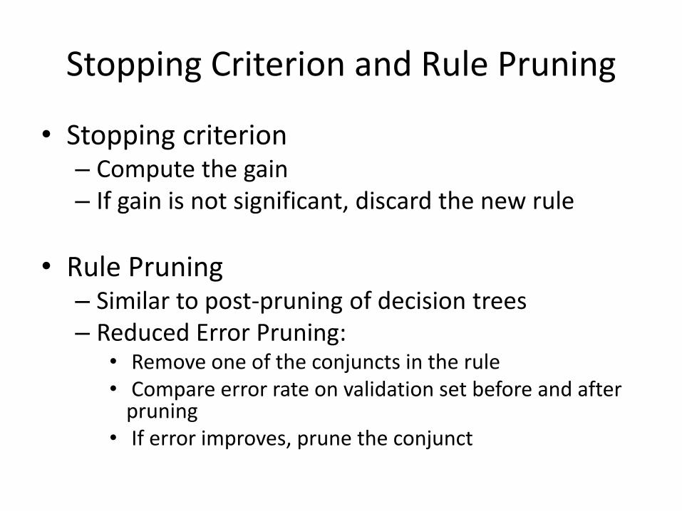
Stopping Criterion and Rule Pruning
• Stopping criterion– Compute the gain– If gain is not significant, discard the new rule
• Rule Pruning– Similar to post-pruning of decision trees– Reduced Error Pruning:
• Remove one of the conjuncts in the rule • Compare error rate on validation set before and after
pruning• If error improves, prune the conjunct

Summary of Direct Method
• Grow a single rule
• Remove Instances from rule
• Prune the rule (if necessary)
• Add rule to Current Rule Set
• Repeat

Direct Method: RIPPER
• For 2-class problem, choose one of the classes as positive class, and the other as negative class
– Learn rules for positive class
– Negative class will be default class
• For multi-class problem
– Order the classes according to increasing class prevalence (fraction of instances that belong to a particular class)
– Learn the rule set for smallest class first, treat the rest as negative class
– Repeat with next smallest class as positive class
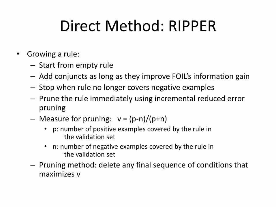
Direct Method: RIPPER
• Growing a rule:
– Start from empty rule
– Add conjuncts as long as they improve FOIL’s information gain
– Stop when rule no longer covers negative examples
– Prune the rule immediately using incremental reduced error pruning
– Measure for pruning: v = (p-n)/(p+n)• p: number of positive examples covered by the rule in
the validation set
• n: number of negative examples covered by the rule inthe validation set
– Pruning method: delete any final sequence of conditions that maximizes v

Direct Method: RIPPER
• Building a Rule Set:– Use sequential covering algorithm
• Finds the best rule that covers the current set of positive examples
• Eliminate both positive and negative examples covered by the rule
– Each time a rule is added to the rule set, compute the new description length• stop adding new rules when the new description
length is d bits longer than the smallest description length obtained so far

Direct Method: RIPPER
• Optimize the rule set:
– For each rule r in the rule set R
• Consider 2 alternative rules:– Replacement rule (r*): grow new rule from scratch
– Revised rule(r’): add conjuncts to extend the rule r
• Compare the rule set for r against the rule set for r* and r’
• Choose rule set that minimizes MDL principle
– Repeat rule generation and rule optimization for the remaining positive examples

Indirect Methods
Rule Set
r1: (P=No,Q=No) ==> -r2: (P=No,Q=Yes) ==> +
r3: (P=Yes,R=No) ==> +
r4: (P=Yes,R=Yes,Q=No) ==> -
r5: (P=Yes,R=Yes,Q=Yes) ==> +
P
Q R
Q- + +
- +
No No
No
Yes Yes
Yes
No Yes

Indirect Method: C4.5rules
• Extract rules from an unpruned decision tree
• For each rule, r: A y, – consider an alternative rule r’: A’ y where A’ is
obtained by removing one of the conjuncts in A
– Compare the pessimistic error rate for r against all r’s
– Prune if one of the r’s has lower pessimistic error rate
– Repeat until we can no longer improve generalization error

Indirect Method: C4.5rules• Instead of ordering the rules, order subsets of
rules (class ordering)
– Each subset is a collection of rules with the same rule consequent (class)
– Compute description length of each subset
• Description length = L(error) + g L(model)
• L(error) is the number of bits needed to encode the misclassified examples, L(model) is the number of bits needed to encode the model
• g is a parameter that takes into account the presence of redundant attributes in a rule set(default value = 0.5)
The class that has the smallest description length is given the highest priority(Occam's Razor)Occam’s Razor: It is a principle urging one to select among competing hypotheses that which makes the fewest assumptions
Recall the regression problem and classification problem:Regularization can prevent over-fitting, why?SVM is the most popular classifier, why?

ExampleName Give Birth Lay Eggs Can Fly Live in Water Have Legs Class
human yes no no no yes mammals
python no yes no no no reptiles
salmon no yes no yes no fishes
whale yes no no yes no mammals
frog no yes no sometimes yes amphibians
komodo no yes no no yes reptiles
bat yes no yes no yes mammals
pigeon no yes yes no yes birds
cat yes no no no yes mammals
leopard shark yes no no yes no fishes
turtle no yes no sometimes yes reptiles
penguin no yes no sometimes yes birds
porcupine yes no no no yes mammals
eel no yes no yes no fishes
salamander no yes no sometimes yes amphibians
gila monster no yes no no yes reptiles
platypus no yes no no yes mammals
owl no yes yes no yes birds
dolphin yes no no yes no mammals
eagle no yes yes no yes birds

C4.5 versus C4.5rules versus RIPPERC4.5rules:
(Give Birth=No, Can Fly=Yes) Birds
(Give Birth=No, Live in Water=Yes) Fishes
(Give Birth=Yes) Mammals
(Give Birth=No, Can Fly=No, Live in Water=No) Reptiles
( ) Amphibians
Give
Birth?
Live In
Water?
Can
Fly?
Mammals
Fishes Amphibians
Birds Reptiles
Yes No
Yes
Sometimes
No
Yes No
RIPPER:
(Live in Water=Yes) Fishes
(Have Legs=No) Reptiles
(Give Birth=No, Can Fly=No, Live In Water=No)
Reptiles
(Can Fly=Yes,Give Birth=No) Birds
() Mammals

C4.5 versus C4.5rules versus RIPPER
PREDICTED CLASS
Amphibians Fishes Reptiles Birds Mammals
ACTUAL Amphibians 0 0 0 0 2
CLASS Fishes 0 3 0 0 0
Reptiles 0 0 3 0 1
Birds 0 0 1 2 1
Mammals 0 2 1 0 4
PREDICTED CLASS
Amphibians Fishes Reptiles Birds Mammals
ACTUAL Amphibians 2 0 0 0 0
CLASS Fishes 0 2 0 0 1
Reptiles 1 0 3 0 0
Birds 1 0 0 3 0
Mammals 0 0 1 0 6
C4.5 and C4.5rules:
RIPPER:
Advantages of Rule-Based Classifiers
• As highly expressive as decision trees
• Easy to interpret
• Easy to generate
• Can classify new instances rapidly
• Performance comparable to decision trees

Instance-Based Classifiers
Atr1 ……... AtrN Class
A
B
B
C
A
C
B
Set of Stored Cases
Atr1 ……... AtrN
Unseen Case
• Store the training records
• Use training records to
predict the class label of
unseen cases

Instance Based Classifiers
• Examples:
– Rote-learner
• Memorizes entire training data and performs classification only if attributes of record match one of the training examples exactly
– Nearest neighbor
• Uses k “closest” points (nearest neighbors) for performing classification

Nearest Neighbor Classifiers
• Basic idea:
– If it walks like a duck, quacks like a duck, then it’s probably a duck
Training
Records
Test
Record
Compute
Distance
Choose k of the
“nearest” records

Nearest-Neighbor Classifiers Requires three things
– The set of stored records
– Distance Metric to compute
distance between records
– The value of k, the number of
nearest neighbors to retrieve
To classify an unknown record:
– Compute distance to other
training records
– Identify k nearest neighbors
– Use class labels of nearest
neighbors to determine the
class label of unknown record
(e.g., by taking majority vote)
Unknown record

Definition of Nearest Neighbor
X X X
(a) 1-nearest neighbor (b) 2-nearest neighbor (c) 3-nearest neighbor
K-nearest neighbors of a record x are data points
that have the k smallest distance to x

1 nearest-neighborVoronoi Diagram
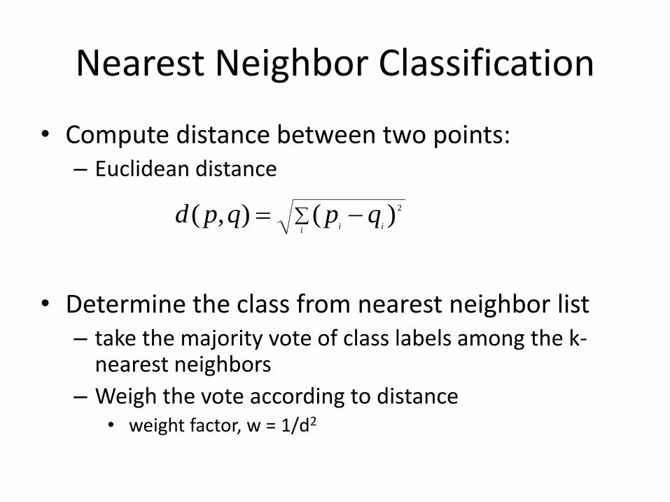
Nearest Neighbor Classification
• Compute distance between two points:– Euclidean distance
• Determine the class from nearest neighbor list– take the majority vote of class labels among the k-
nearest neighbors
– Weigh the vote according to distance• weight factor, w = 1/d2
i ii
qpqpd 2)(),(

Nearest Neighbor Classification…
• Choosing the value of k:– If k is too small, sensitive to noise points
– If k is too large, neighborhood may include points from other classes
X

Nearest Neighbor Classification…
• Scaling issues
– Attributes may have to be scaled to prevent distance measures from being dominated by one of the attributes
– Example:
• height of a person may vary from 1.5m to 1.8m
• weight of a person may vary from 90lb to 300lb
• income of a person may vary from $10K to $1M

Nearest Neighbor Classification…
• Problem with Euclidean measure:
– High dimensional data
• curse of dimensionality
– Can produce counter-intuitive results1 1 1 1 1 1 1 1 1 1 1 0
0 1 1 1 1 1 1 1 1 1 1 1
1 0 0 0 0 0 0 0 0 0 0 0
0 0 0 0 0 0 0 0 0 0 0 1
vs
d = 1.4142 d = 1.4142
Solution: Normalize the vectors to unit length

Nearest neighbor Classification…
• k-NN classifiers are lazy learners
– It does not build models explicitly
– Unlike eager learners such as decision tree induction and rule-based systems
– Classifying unknown records are relatively expensive

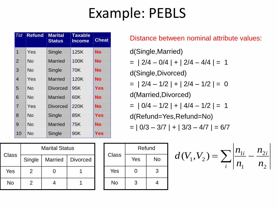
Example: PEBLS
• PEBLS: Parallel Examplar-Based Learning System (Cost & Salzberg)
– Works with both continuous and nominal features
• For nominal features, distance between two nominal values is computed using modified value difference metric (MVDM)
– Each record is assigned a weight factor
– Number of nearest neighbor, k = 1
Example: PEBLS
Class
Refund
Yes No
Yes 0 3
No 3 4
Class
Marital Status
Single Married Divorced
Yes 2 0 1
No 2 4 1
i
ii
n
n
n
nVVd
2
2
1
121 ),(
Distance between nominal attribute values:
d(Single,Married)
= | 2/4 – 0/4 | + | 2/4 – 4/4 | = 1
d(Single,Divorced)
= | 2/4 – 1/2 | + | 2/4 – 1/2 | = 0
d(Married,Divorced)
= | 0/4 – 1/2 | + | 4/4 – 1/2 | = 1
d(Refund=Yes,Refund=No)
= | 0/3 – 3/7 | + | 3/3 – 4/7 | = 6/7
Tid Refund MaritalStatus
TaxableIncome Cheat
1 Yes Single 125K No
2 No Married 100K No
3 No Single 70K No
4 Yes Married 120K No
5 No Divorced 95K Yes
6 No Married 60K No
7 Yes Divorced 220K No
8 No Single 85K Yes
9 No Married 75K No
10 No Single 90K Yes10

Example: PEBLSTid Refund Marital
Status Taxable Income Cheat
X Yes Single 125K No
Y No Married 100K No 10
d
i
iiYX YXdwwYX1
2),(),(
Distance between record X and record Y:
where:
correctly predicts X timesofNumber
predictionfor used is X timesofNumber Xw
wX 1 if X makes accurate prediction most of the time
wX > 1 if X is not reliable for making predictions
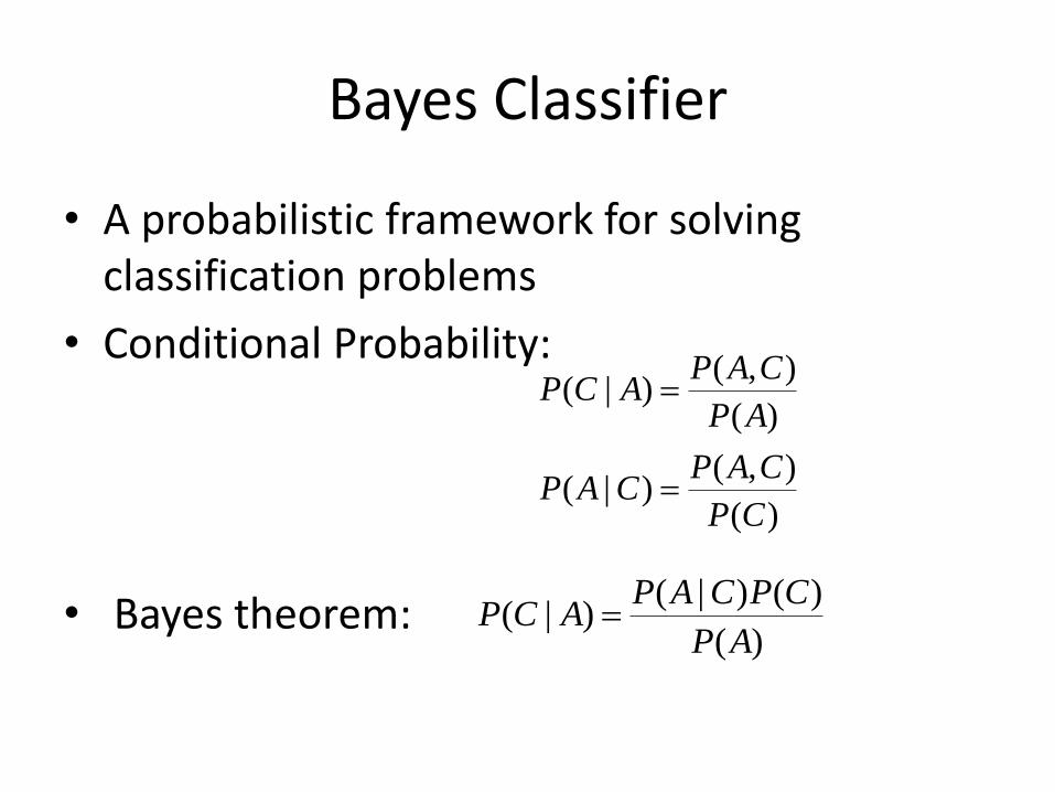
Bayes Classifier
• A probabilistic framework for solving classification problems
• Conditional Probability:
• Bayes theorem:)(
)()|()|(
AP
CPCAPACP
)(
),()|(
)(
),()|(
CP
CAPCAP
AP
CAPACP
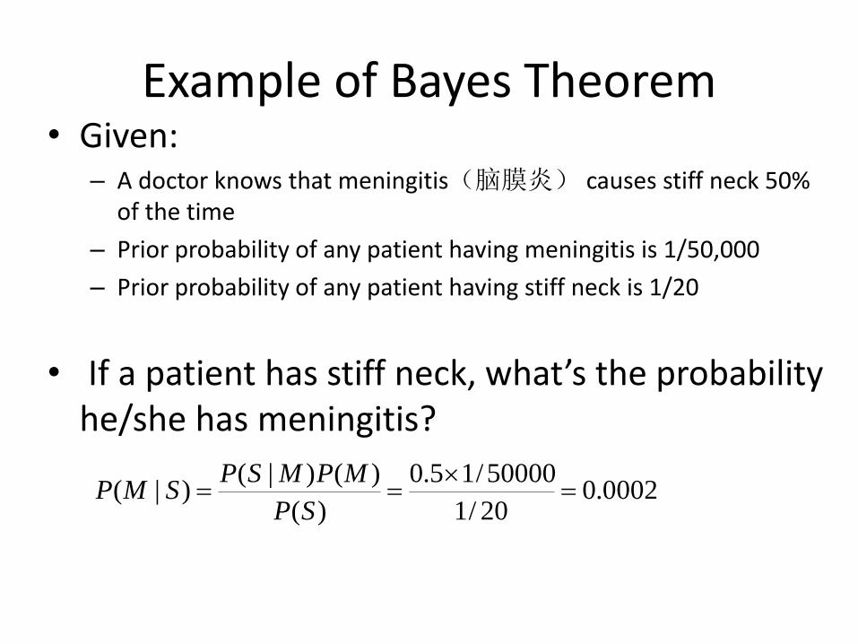
Example of Bayes Theorem• Given:
– A doctor knows that meningitis(脑膜炎) causes stiff neck 50% of the time
– Prior probability of any patient having meningitis is 1/50,000
– Prior probability of any patient having stiff neck is 1/20
• If a patient has stiff neck, what’s the probability he/she has meningitis?
0002.020/1
50000/15.0
)(
)()|()|(
SP
MPMSPSMP

Bayesian Classifiers• Consider each attribute and class label as
random variables
• Given a record with attributes (A1, A2,…,An) – Goal is to predict class C
– Specifically, we want to find the value of C that maximizes P(C| A1, A2,…,An )
• Can we estimate P(C| A1, A2,…,An ) directly from data?

Bayesian Classifiers• Approach:
– compute the posterior probability P(C | A1, A2, …, An) for all values of C using the Bayes theorem
– Choose value of C that maximizes P(C | A1, A2, …, An)
– Equivalent to choosing value of C that maximizesP(A1, A2, …, An|C) P(C)
• How to estimate P(A1, A2, …, An | C )?
)(
)()|()|(
21
21
21
n
n
n
AAAP
CPCAAAPAAACP

Naïve Bayes Classifier
• Assume independence among attributes Ai when class is given:
– P(A1, A2, …, An |C) = P(A1| Cj) P(A2| Cj)… P(An| Cj)
– Can estimate P(Ai| Cj) for all Ai and Cj.
– New point is classified to Cj if P(Cj) P(Ai| Cj) is maximal.

How to Estimate Probabilities from Data?
• Class: P(C) = Nc/N– e.g., P(No) = 7/10,
P(Yes) = 3/10
• For discrete attributes:
P(Ai | Ck) = |Aik|/ Nc
– where |Aik| is number of instances having attribute Ai
and belongs to class Ck
– Examples:
P(Status=Married|No) = 4/7P(Refund=Yes|Yes)=0
k
Tid Refund Marital Status
Taxable Income Evade
1 Yes Single 125K No
2 No Married 100K No
3 No Single 70K No
4 Yes Married 120K No
5 No Divorced 95K Yes
6 No Married 60K No
7 Yes Divorced 220K No
8 No Single 85K Yes
9 No Married 75K No
10 No Single 90K Yes 10
categoric
al
categoric
al
continuous
class

How to Estimate Probabilities from Data?
• For continuous attributes: – Discretize the range into bins
• one ordinal attribute per bin• violates independence assumption
– Two-way split: (A < v) or (A > v)• choose only one of the two splits as new attribute
– Probability density estimation:• Assume attribute follows a normal distribution• Use data to estimate parameters of distribution
(e.g., mean and standard deviation)• Once probability distribution is known, can use it to
estimate the conditional probability P(Ai|c)
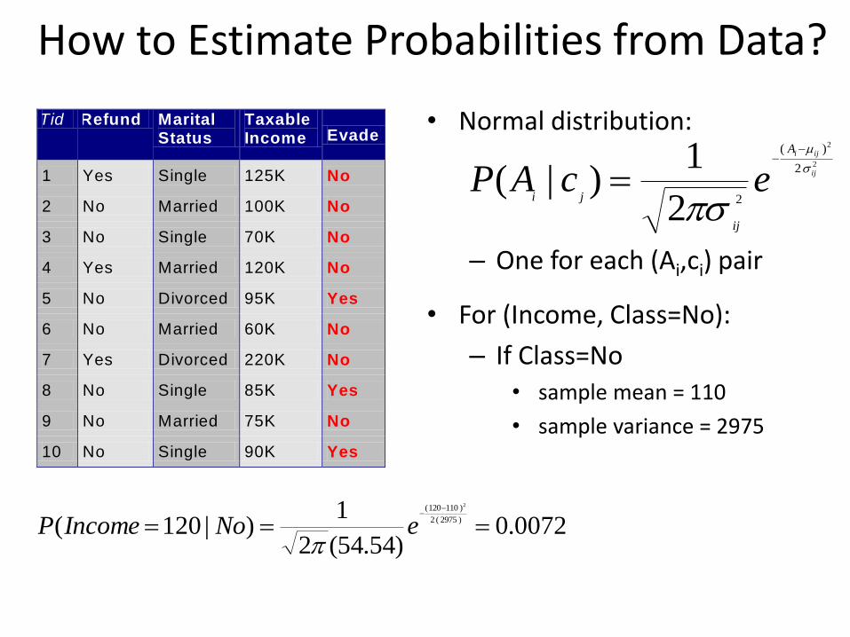
How to Estimate Probabilities from Data?
• Normal distribution:
– One for each (Ai,ci) pair
• For (Income, Class=No):
– If Class=No• sample mean = 110
• sample variance = 2975
Tid Refund Marital Status
Taxable Income Evade
1 Yes Single 125K No
2 No Married 100K No
3 No Single 70K No
4 Yes Married 120K No
5 No Divorced 95K Yes
6 No Married 60K No
7 Yes Divorced 220K No
8 No Single 85K Yes
9 No Married 75K No
10 No Single 90K Yes 10
categoric
al
categoric
al
continuous
class
2
2
2
)(
22
1)|( ij
ijiA
ij
jiecAP
0072.0)54.54(2
1)|120( )2975(2
)110120( 2
eNoIncomeP

Example of Naïve Bayes Classifier
P(Refund=Yes|No) = 3/7
P(Refund=No|No) = 4/7
P(Refund=Yes|Yes) = 0
P(Refund=No|Yes) = 1
P(Marital Status=Single|No) = 2/7
P(Marital Status=Divorced|No)=1/7
P(Marital Status=Married|No) = 4/7
P(Marital Status=Single|Yes) = 2/7
P(Marital Status=Divorced|Yes)=1/7
P(Marital Status=Married|Yes) = 0
For taxable income:
If class=No: sample mean=110
sample variance=2975
If class=Yes: sample mean=90
sample variance=25
naive Bayes Classifier:
120K)IncomeMarried,No,Refund( X
P(X|Class=No) = P(Refund=No|Class=No)
P(Married| Class=No)
P(Income=120K| Class=No)
= 4/7 4/7 0.0072 = 0.0024
P(X|Class=Yes) = P(Refund=No| Class=Yes)
P(Married| Class=Yes)
P(Income=120K| Class=Yes)
= 1 0 1.2 10-9 = 0
Since P(X|No)P(No) > P(X|Yes)P(Yes)
Therefore P(No|X) > P(Yes|X)
=> Class = No
Given a Test Record:

Naïve Bayes Classifier
• If one of the conditional probability is zero, then the entire expression becomes zero
• Probability estimation:
cN
NCAP
N
NCAP
c
ici
c
ici
1)|(:Laplace
)|( :Originalc: number of classes
p: prior probability
m: parameter

Example of Naïve Bayes ClassifierName Give Birth Can Fly Live in Water Have Legs Class
human yes no no yes mammals
python no no no no non-mammals
salmon no no yes no non-mammals
whale yes no yes no mammals
frog no no sometimes yes non-mammals
komodo no no no yes non-mammals
bat yes yes no yes mammals
pigeon no yes no yes non-mammals
cat yes no no yes mammals
leopard shark yes no yes no non-mammals
turtle no no sometimes yes non-mammals
penguin no no sometimes yes non-mammals
porcupine yes no no yes mammals
eel no no yes no non-mammals
salamander no no sometimes yes non-mammals
gila monster no no no yes non-mammals
platypus no no no yes mammals
owl no yes no yes non-mammals
dolphin yes no yes no mammals
eagle no yes no yes non-mammals
Give Birth Can Fly Live in Water Have Legs Class
yes no yes no ?
0027.020
13004.0)()|(
021.020
706.0)()|(
0042.013
4
13
3
13
10
13
1)|(
06.07
2
7
2
7
6
7
6)|(
NPNAP
MPMAP
NAP
MAP
A: attributes
M: mammals
N: non-mammals
P(A|M)P(M) > P(A|N)P(N)
=> Mammals

Naïve Bayes (Summary)
• Robust to isolated noise points
• Handle missing values by ignoring the instance during probability estimate calculations
• Robust to irrelevant attributes
• Independence assumption may not hold for some attributes– Use other techniques such as Bayesian Belief
Networks (BBN)
63
Ensemble Classifier

A very important method
• All the competitors of data mining competition, such as KDD CUP, adopt ensemble methods to enhance the performance of their algorithm.
64

65
General Idea
Original
Training data
....D
1D
2 Dt-1
Dt
D
Step 1:
Create Multiple
Data Sets
C1
C2
Ct -1
Ct
Step 2:
Build Multiple
Classifiers
C*
Step 3:
Combine
Classifiers

66
Why does it work?
• Suppose there are 25 base classifiers
– Each classifier has error rate, = 0.35
– Assume classifiers are independent
– Probability that the ensemble classifier makes a wrong prediction:
25
13
25 06.0)1(25
i
ii
i

67
Examples of Ensemble Methods
• How to generate an ensemble of classifiers?
– Bagging
– Boosting

68
Bagging
• Sampling with replacement
• Build classifier on each bootstrap sample
• Each sample has probability (1 – 1/n)n of not being selected as training data
• Training data = 1- (1 – 1/n)n of the original data
Original Data 1 2 3 4 5 6 7 8 9 10
Bagging (Round 1) 7 8 10 8 2 5 10 10 5 9
Bagging (Round 2) 1 4 9 1 2 3 2 7 3 2
Bagging (Round 3) 1 8 5 10 5 5 9 6 3 7
Training DataData ID
6969
The 0.632 bootstrap
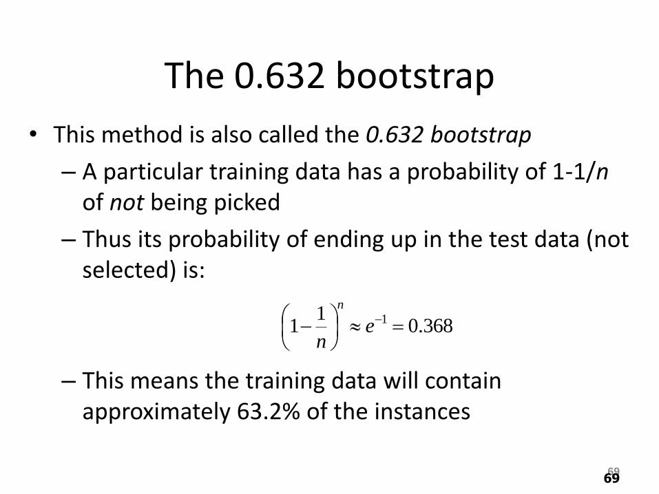
• This method is also called the 0.632 bootstrap
– A particular training data has a probability of 1-1/nof not being picked
– Thus its probability of ending up in the test data (not selected) is:
– This means the training data will contain approximately 63.2% of the instances
368.01
1 1
e
n
n

70
Bagging (applied to training data)
Accuracy of ensemble classifier: 100%

71
Bagging- Summary
• Works well if the base classifiers are unstable (complement each other)
• Increased accuracy because it reduces the variance of the individual classifier
• Does not focus on any particular instance of the training data– Therefore, less susceptible to model over-fitting when
applied to noisy data
• What if we want to focus on a particular instances of training data?
72
Boosting
• An iterative procedure to adaptively change distribution of training data by focusing more on previously misclassified records
– Initially, all N records are assigned equal weights
– Unlike bagging, weights may change at the end of a boosting round

73
Boosting
• Records that are wrongly classified will have their weights increased
• Records that are classified correctly will have their weights decreased
Original Data 1 2 3 4 5 6 7 8 9 10
Boosting (Round 1) 7 3 2 8 7 9 4 10 6 3
Boosting (Round 2) 5 4 9 4 2 5 1 7 4 2
Boosting (Round 3) 4 4 8 10 4 5 4 6 3 4
• Example 4 is hard to classify
• Its weight is increased, therefore it is more likely to be chosen again in subsequent rounds

74
Boosting
• Equal weights are assigned to each training instance (1/N for round 1) at first round
• After a classifier Ci is learned, the weights are adjusted to allow the subsequent classifier
Ci+1 to “pay more attention” to data that were misclassified by Ci.
• Final boosted classifier C* combines the votes of each individual classifier– Weight of each classifier’s vote is a function of its
accuracy
• Adaboost – popular boosting algorithm

75
Adaboost (Adaptive Boost)
• Input:
– Training set D containing N instances
– T rounds
– A classification learning scheme
• Output:
– A composite model

76
Adaboost: Training Phase
• Base classifier Ci, is derived from training data of Di
• Error of Ci is tested using Di
• Weights of training data are adjusted depending on how they were classified
– Correctly classified: Decrease weight
– Incorrectly classified: Increase weight
• Weight of a data indicates how hard it is to classify it (directly proportional)

77
Adaboost: Training Phase
• Training data D contain N labeled data (X1,y1), (X2,y2 ), (X3,y3),….(XN,yN)
• Initially assign equal weight 1/N to each data• To generate T base classifiers, we need T rounds or
iterations• Round i, data from D are sampled with replacement ,
to form Di (size N)• Each data’s chance of being selected in the next
rounds depends on its weight– Each time the new sample is generated directly from the
training data D with different sampling probability according to the weights; these weights are not zero

78
Adaboost: Testing Phase
• The lower a classifier error rate, the more accurate it is, and therefore, the higher its weight for voting should be
• Weight of a classifier Ci’s vote is
• Testing: – For each class c, sum the weights of each classifier that assigned class c to
X (unseen data)
– The class with the highest sum is the WINNER!
i
ii
1ln
2
1
T
i
testiiy
test yxCxC1
)(maxarg)(*

79
Example: Error and Classifier Weight in AdaBoost
• Base classifiers: C1, C2, …, CT
• Error rate: (i = index of classifier, j=index of instance)
• Importance of a classifier:
N
j
jjiji yxCwN 1
)(1
i
ii
1ln
2
1

80
Example: Data Instance Weight in AdaBoost• Assume: N training data in D, T rounds, (xj,yj) are
the training data, Ci, ai are the classifier and weight of the ith round, respectively.
• Weight update on all training data in D:
factorion normalizat theis where
)( ifexp
)( ifexp)(
)1(
i
jji
jji
i
i
ji
j
Z
yxC
yxC
Z
ww
i
i
T
i
testiiy
test yxCxC1
)(maxarg)(*

81
Boosting
Round 1 + + + -- - - - - -0.0094 0.0094 0.4623
B1
= 1.9459
Illustrating AdaBoostData points for training
Initial weights for each data point
Original
Data + + + -- - - - + +
0.1 0.1 0.1

82
Illustrating AdaBoostBoosting
Round 1 + + + -- - - - - -
Boosting
Round 2 - - - -- - - - + +
Boosting
Round 3 + + + ++ + + + + +
Overall + + + -- - - - + +
0.0094 0.0094 0.4623
0.3037 0.0009 0.0422
0.0276 0.1819 0.0038
B1
B2
B3
= 1.9459
= 2.9323
= 3.8744

不平衡类问题
• 在许多实际应用具有不平衡类分布的数据集的问题– 监管产品生产线的下线产品自动检测系统会发现:不合格产品的数量
远远低于合格产品数量
– 信用卡欺诈检测中,合法交易远远多于欺诈交易
• 在这些应用中,稀有类的正确分类比多数类的正确分类更有价值。这给已有的分类算法带来了很多问题– 因稀有类的实例很少出现,描述稀有类的模型趋向会变得高度特殊化
– 例如,在基于规则的分类器中,为稀有类提取的规则通常涉及大量的属性,并很难简化为更一般的、具有很高覆盖率的规则(不像关于多数类的规则)。模型也很容易受到训练数据中噪声的影响。
– 许多已有的算法不能很好的检测稀有类的实例

Metrics for Performance Evaluation
• 由于准确率将每个类等同重要看待,因此不太适用于不平衡数据集。在不平衡数据集中,稀有类比多数类更有意义。
• 稀有类比多数类更有意义。为此,对于二元分类,通常将稀有类标记为正类,而多数类标记为负类。

Metrics for Performance Evaluation
• Focus on the predictive capability of a model
– Rather than how fast it takes to classify or build models, scalability, etc.
• Confusion Matrix (混淆矩阵):
PREDICTED CLASS
ACTUAL
CLASS
Class=Yes Class=No
Class=Yes a b
Class=No c d
a: TP (true positive)
b: FN (false negative)
c: FP (false positive)
d: TN (true negative)

Metrics for Performance Evaluation…
• Most widely-used metric:
PREDICTED CLASS
ACTUAL
CLASS
Class=Yes Class=No
Class=Yes + f++ (TP) f+- (FN)
Class=No - f-+ (FP) f-- (TN)
Accuracy f f TP TN
f f f f TP TN FP FN

Limitation of Accuracy
• Consider a 2-class problem
– Number of Class 0 examples = 9990
– Number of Class 1 examples = 10
• If model predicts everything to be class 0, accuracy is 9990/10000 = 99.9 %
– Accuracy is misleading because model does not detect any class 1 example

Metrics for Performance Evaluation
• 混淆矩阵中的计数可以表示为百分比的形式。– 真正率(true positive rate, TPR)或敏感度(sensitivity)定义为被模
型正确预测的正样本的比例,即:
TPR = TP/(TP+FN)
– 真负率(true negative rate, TPR)或特指度(specificity)定义为被模型正确预测的负样本的比例,即:
TNR = TN/(TN+FP)
– 假正率(false positive rate, TPR)或特指度(specificity)定义为被模型预测为正类的负样本的比例,即:
FPR = FP/(TN+FP)
– 假负率(false negative rate, FNR)定义为被模型预测为负类的正样本比例,即:
FNR = FN/(TP+FN)
Metrics for Performance Evaluation
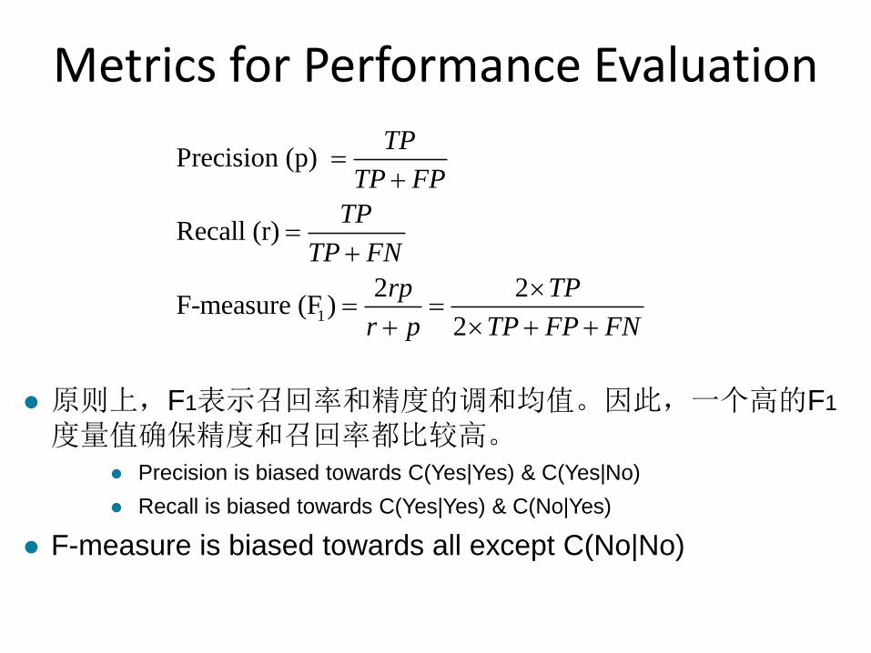
1
Precision (p)
Recall (r)
2 2F-measure (F )
2
TP
TP FP
TP
TP FN
rp TP
r p TP FP FN
原则上,F1表示召回率和精度的调和均值。因此,一个高的F1
度量值确保精度和召回率都比较高。 Precision is biased towards C(Yes|Yes) & C(Yes|No)
Recall is biased towards C(Yes|Yes) & C(No|Yes)
F-measure is biased towards all except C(No|No)

Metrics for Performance Evaluation
1 4
1 2 3 4
Weighted Accuracy wTP w TN
wTP w FP w FN w TN
• 更一般的,可以用 度量考察召回率和精度之间的折中
• 精度和召回率分别是 = 0和 = 时 的特例。低 值使得 接近于精度,高 值使得 值接近于召回率。
• 更一般的,捕获 值和准确率的度量是加权准确率度量,由下式定义:
2
2
( 1)rpF
r p
F
F
FF

ROC (Receiver Operating Characteristic)
• Developed in 1950s for signal detection theory to analyze noisy signals– Characterize the trade-off between positive hits and false
alarms
• ROC curve plots TPR (on the y-axis) against FPR (on the x-axis)
• Performance of each classifier represented as a point on the ROC curve– changing the threshold of algorithm, sample distribution or
cost matrix changes the location of the point

ROC Curve
At threshold t:
TP=0.5, FN=0.5, FP=0.12, TN=0.88
- 1-dimensional data set containing 2 classes (positive and negative)
- any points located at x > t is classified as positive

ROC Curve(TP,FP):
• (0,0): declare everythingto be negative class
• (1,1): declare everythingto be positive class
• (1,0): ideal
• Diagonal line:
– Random guessing
– Below diagonal line:• prediction is opposite of the
true class

Using ROC for Model Comparison No model consistently
outperform the other
M1 is better for
small FPR
M2 is better for
large FPR
Area Under the ROC
curve
Ideal:
Area = 1
Random guess:
Area = 0.5
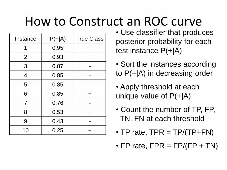
How to Construct an ROC curveInstance P(+|A) True Class
1 0.95 +
2 0.93 +
3 0.87 -
4 0.85 -
5 0.85 -
6 0.85 +
7 0.76 -
8 0.53 +
9 0.43 -
10 0.25 +
• Use classifier that produces
posterior probability for each
test instance P(+|A)
• Sort the instances according
to P(+|A) in decreasing order
• Apply threshold at each
unique value of P(+|A)
• Count the number of TP, FP,
TN, FN at each threshold
• TP rate, TPR = TP/(TP+FN)
• FP rate, FPR = FP/(FP + TN)

How to construct an ROC curveClass + - + - - - + - + +
P 0.25 0.43 0.53 0.76 0.85 0.85 0.85 0.87 0.93 0.95 1.00
TP 5 4 4 3 3 3 3 2 2 1 0
FP 5 5 4 4 3 2 1 1 0 0 0
TN 0 0 1 1 2 3 4 4 5 5 5
FN 0 1 1 2 2 2 2 3 3 4 5
TPR 1 0.8 0.8 0.6 0.6 0.6 0.6 0.4 0.4 0.2 0
FPR 1 1 0.8 0.8 0.6 0.4 0.2 0.2 0 0 0
Threshold >=
ROC Curve:

Cost Matrix
PREDICTED CLASS
ACTUAL
CLASS
C(i|j) Class=Yes Class=No
Class=Yes C(Yes|Yes) C(No|Yes)
Class=No C(Yes|No) C(No|No)
C(i|j): Cost of misclassifying class j example as class i
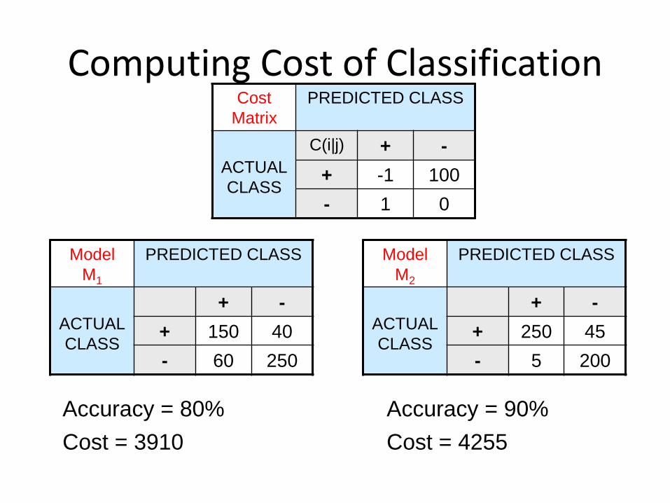
Computing Cost of ClassificationCost
Matrix
PREDICTED CLASS
ACTUAL
CLASS
C(i|j) + -
+ -1 100
- 1 0
Model
M1
PREDICTED CLASS
ACTUAL
CLASS
+ -
+ 150 40
- 60 250
Model
M2
PREDICTED CLASS
ACTUAL
CLASS
+ -
+ 250 45
- 5 200
Accuracy = 80%
Cost = 3910
Accuracy = 90%
Cost = 4255

Cost vs Accuracy
Count PREDICTED CLASS
ACTUAL
CLASS
Class=Yes Class=No
Class=Yes a b
Class=No c d
Cost PREDICTED CLASS
ACTUAL
CLASS
Class=Yes Class=No
Class=Yes p q
Class=No q p
N = a + b + c + d
Accuracy = (a + d)/N
Cost = p (a + d) + q (b + c)
= p (a + d) + q (N – a – d)
= q N – (q – p)(a + d)
= N [q – (q-p) Accuracy]
Accuracy is proportional to cost if
1. C(Yes|No)=C(No|Yes) = q
2. C(Yes|Yes)=C(No|No) = p


