Download - Chap. 14: Nonparametric Statistics

Non-Parametric Statistics
Rupika Abeynayake, Ph.D (Statistics)
Professor in Applied Statistics

Content
Introduction: Distribution-Free Tests
Single Population Inferences
Comparing Two Populations:
Independent Samples
Comparing Two Populations: Paired
Difference Experiment
Comparing Three or More
Populations: Completely Randomized
Design

Content
Comparing Three or More
Populations: Randomized Block Design
Rank Correlation

Learning Objectives
• Develop the need for inferential
techniques that require fewer, or less
stringent, assumptions than parametric
methods
• Introduce nonparametric tests that are
based on ranks (i.e., on an ordering of
the sample measurements according to
their relative magnitudes)

Introduction:
Distribution-Free Tests

Parametric Test Procedures
• Involve population parameters— Example: population mean
• Require interval scale or ratio scale— Whole numbers or fractions
— Example: height in inches (72, 60.5, 54.7)
• Have stringent assumptions— Example: normal distribution
• Examples: z-test, t-test, F-test, 2-test
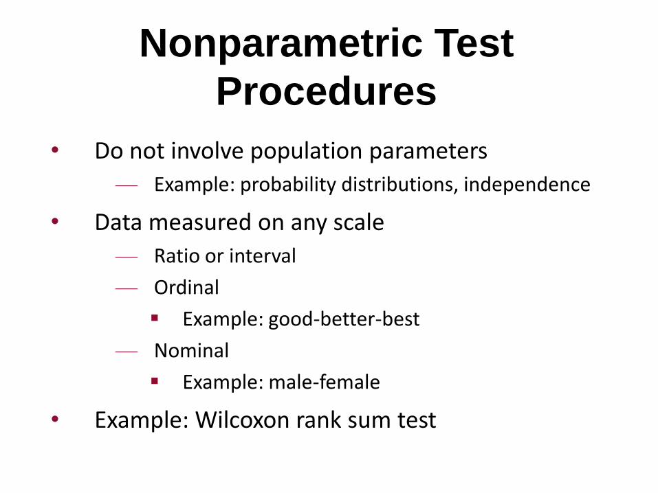
Nonparametric Test
Procedures
• Do not involve population parameters
— Example: probability distributions, independence
• Data measured on any scale
— Ratio or interval
— Ordinal
Example: good-better-best
— Nominal
Example: male-female
• Example: Wilcoxon rank sum test

Nonnormal Distributions -
t-Statistic is Invalid
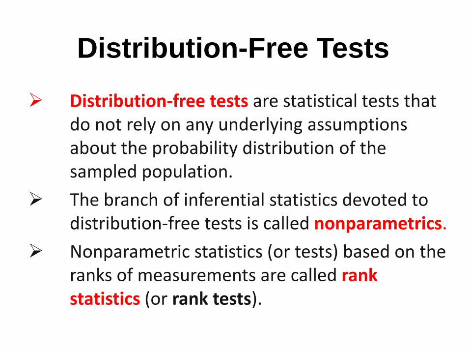
Distribution-Free Tests
Distribution-free tests are statistical tests that do not rely on any underlying assumptions about the probability distribution of the sampled population.
The branch of inferential statistics devoted to distribution-free tests is called nonparametrics.
Nonparametric statistics (or tests) based on the ranks of measurements are called rank statistics (or rank tests).

Advantages of
Nonparametric Tests
• Used with all scales
• Easier to compute
• Make fewer assumptions
• Need not involve population parameters
• Results may be as exact as parametric procedures

Disadvantages of
Nonparametric Tests• May waste information
— If data permit using parametric procedures
— Example: converting data from ratio to ordinal scale
• Difficult to compute by hand for large samples
• Tables not widely available
• Power of the test is low
• It is merely for testing of hypothesis and no confidence limits could be calculated.

Frequently Used Nonparametric
Tests
• Sign Test
• Wilcoxon Signed Rank Test
• Wilcoxon Rank Sum Test – Mann-Whitny test
• Kruskal Wallis H-Test – Quade test
• Friedman test
• Spearman’s Rank Correlation Coefficient© 2011 Pearson Education, Inc
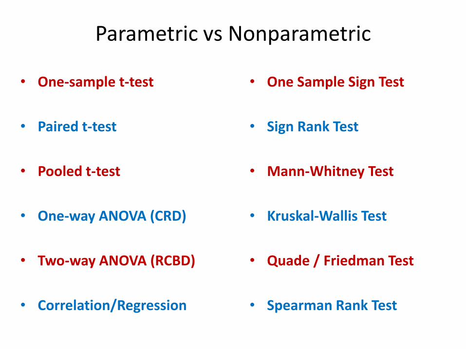
Parametric vs Nonparametric
• One Sample Sign Test
• Sign Rank Test
• Mann-Whitney Test
• Kruskal-Wallis Test
• Quade / Friedman Test
• Spearman Rank Test
• One-sample t-test
• Paired t-test
• Pooled t-test
• One-way ANOVA (CRD)
• Two-way ANOVA (RCBD)
• Correlation/Regression

Single Population Inferences

Sign Test
• Tests one population median, (eta)
• Corresponds to t-test for one mean
• Assumes population is continuous
• Small sample test statistic: Number of sample values above (or below) median
• Can use normal approximation if n 30

Sign Test Uses p-Value
to Make Decision
.031
.109
.219
.273
.219
.109
.031.004.004
0%
10%
20%
30%
0 1 2 3 4 5 6 7 8 X
P(X)
© 2011 Pearson Education, Inc
Binomial: n = 8 p = 0.5
P-value is the probability of getting an observation at least as
extreme as we got. If 7 of 8 observations ‘favor’ Ha, then
p-value = p(x 7) = .031 + .004 = .035.
If = .05, then reject H0 since p-value .

Sign Test for a Population
Median
One-Tailed Test
H0: = 0
Ha: > 0 [or Ha: < 0 ]
Test statistic:
S = Number of sample measurements greater than0 [or S = number of measurements less than 0]

Sign Test Example
You’re an analyst for a some fruit juice company. You’ve asked 7 people to rate a new fruit juice on a 5-point Likert scale (1 = terrible to 5 = excellent). The ratings are:
2 5 4 4 1 4 5
At the .05 level of significance, is there evidence that the median rating is greater than 3?

Sign Test Solution
• H0:
• Ha:
• =
• Test Statistic:
© 2011 Pearson Education, Inc
p-value:
Decision:
Conclusion:
Do not reject null
hypothesis at = .05
There is no evidence
median is greater than 3
P(x 5) = 1 – P(x 4)
= 1-0.7734
=0.2266
S = 5
(Ratings 1 & 2 are
less than = 3:
2, 5, 4, 4, 1, 4, 5)
= 3
> 3
.05

Sign Test for a Population
Median
Observed significance level:
p-value = P(x ≥ S)
where x has a binomial distribution with parameters n and p = .5
Rejection region: Reject H0 if p-value ≤ .05

Sign Test for a Population
Median
Two-Tailed Test
H0: = 0
Ha: ≠ 0
Test statistic:
S = Larger of S1 and S2, where S1 is the number of sample measurements less than0 and S2 is the number of measurements greater than 0

Sign Test for a Population
Median
Observed significance level:
p-value = 2P(x ≥ S)
where x has a binomial distribution with parameters n and p = .5
Rejection region: Reject H0 if p-value ≤ .05

Recent studies of the private practices of physicians
who saw no Medicaid patients suggested that the
median length of each patient visit was 22 minutes. It is
believed that the median visit length in practices with a
large Medicaid load is shorter than 22 minutes. A
random sample of 20 visits in practices with a large
Medicaid load yielded, in order, the following visit
lengths:
9.4 13.4 15.6 16.2 16.4 16.8
18.1 18.7 18.9 19.1 19.3 20.1
20.4 21.6 21.9 23.4 23.5 24.8
24.9 26.8
Based on these data, is there sufficient evidence to conclude that
the median visit length in practices with a large Medicaid load is
shorter than 22 minutes?
Conditions Required for Valid
Application of the Sign Test
The sample is selected randomly from a continuous probability distribution
[Note: No assumptions need to be made about the shape of the probability distribution.]

Large Sample Sign Test for a
Population Median
One-Tailed TestH0: = 0Ha: > 0 [or Ha: < 0 ]
Test statistic:
N is the number of sample not equal to the hypnotized valueS = Number of sample measurements greater than0 [or S = number of measurements less than 0] The “– .5” is the “correction for continuity.”
z
S .5 .5n
.5 n
Can use normal approximation if n 30

Large Sample Sign Test for a
Population Median
The null hypothesized mean value is np = .5n, and the standard deviation is
Rejection region: z > z
npq n .5 .5 .5 n

Large Sample Sign Test for a
Population Median
Two-Tailed Test
H0: = 0
Ha: ≠ 0
Test statistic:
S = Larger of S1 and S2, where S1 is the number of sample measurements less than0 and S2 is the number of measurements greater than 0
© 2011 Pearson Education, Inc
z
S .5 .5n
.5 n

Large Sample Sign Test for a
Population Median
The null hypothesized mean value is np = .5n, and the standard deviation is
Rejection region: z > z
npq n .5 .5 .5 n

The Gordon Travel Agency claims that their median airfare for
all their clients to all destinations is $450.
This claim is being challenged by a competing agency, who
believe the median is different from $450.
A random sample of 300 tickets revealed
170 tickets were below $450. Use the 0.05 level of
significance.

Continued…
H0 is rejected if z is > than 1.96 or < than -1.96
… the value of z is 2.252
H0 is rejected.
We conclude that the median is not $450
450$median :H$450=median : 10H
252.23005.
)300(50.)5.170(
5.
50.)5.(
n
nxz
Comparing Two Populations:Related Samples
Wilcoxon signed rank test
To test difference between paired data

Example
Data
14
2
5
4
2
14
18
14
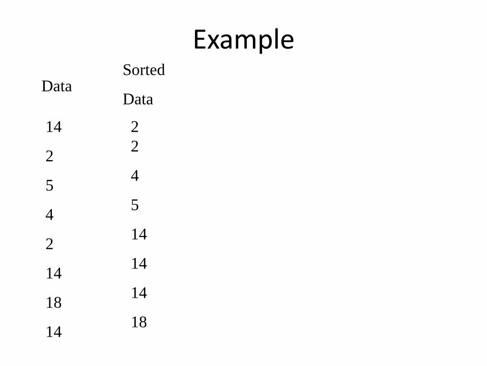
ExampleSorted
Data
2
2
4
5
14
14
14
18
Data
14
2
5
4
2
14
18
14

ExampleSorted
Data
2
2
4
5
14
14
14
18
Data
14
2
5
4
2
14
18
14
TIES

ExampleSorted
Data
2
2
4
5
14
14
14
18
Data
14
2
5
4
2
14
18
14
TIES
Rank them
anyway,
pretending they
were slightly
different

Example
Rank A
2
2
4
5
14
14
14
18
1
2
3
4
5
6
7
8
Sorted
DataData
14
2
5
4
2
14
18
14

Example
Rank A
2
2
4
5
14
14
14
18
1
2
3
4
5
6
7
8
Sorted
DataData
14
2
5
4
2
14
18
14
Find the
average of the
ranks for the
identical
values, and give
them all that
rank

Example
Rank A
2
2
4
5
14
14
14
18
1
2
3
4
5
6
7
8
Sorted
DataData
14
2
5
4
2
14
18
14
Average = 1.5
Average = 6

Example
Rank A
2
2
4
5
14
14
14
18
1
2
3
4
5
6
7
8
Sorted
DataData
14
2
5
4
2
14
18
14
1.5
1.5
3
4
6
6
6
8
Rank

Example
Rank A
2
2
4
5
14
14
14
18
1
2
3
4
5
6
7
8
Sorted
DataData
14
2
5
4
2
14
18
14
1.5
1.5
3
4
6
6
6
8
Rank
These can now be used for the Mann-Whitney U test

Patient
Hours of sleep
Drug Placebo
1 6.1 5.2
2 7.0 7.9
3 8.2 3.9
4 7.6 4.7
5 6.5 5.3
6 8.4 5.4
7 6.9 4.2
8 6.7 6.1
9 7.4 3.8
10 5.8 6.3
EXAMPLE
Null Hypothesis: Hours of sleep are the same using placebo & the drug

STEP 1• Exclude any differences which are zero
• Ignore their signs
• Put the rest of differences in ascending order
• Assign them ranks
• If any differences are equal, average their
ranks

STEP 2
• Count up the ranks of +ives as W+
• Count up the ranks of –ives as W-

STEP 3• If there is no difference between drug (W+)
and placebo (W-), then W+ & W- would be similar
• If there is a difference
one sum would be much smaller and
the other much larger than expected
• The smaller sum is denoted as W
• W = smaller of W+ and W-
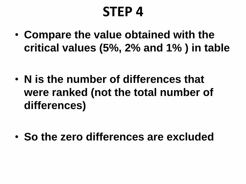
STEP 4
• Compare the value obtained with the
critical values (5%, 2% and 1% ) in table
• N is the number of differences that
were ranked (not the total number of
differences)
• So the zero differences are excluded

Patient
Hours of sleep
Difference
Rank
Ignoring signDrug Placebo
1 6.1 5.2 0.9 3.5*
2 7.0 7.9 -0.9 -3.5*
3 8.2 3.9 4.3 10
4 7.6 4.7 2.9 7
5 6.5 5.3 1.2 5
6 8.4 5.4 3.0 8
7 6.9 4.2 2.7 6
8 6.7 6.1 0.6 2
9 7.4 3.8 3.6 9
10 5.8 6.3 -0.5 -1
3rd & 4th ranks are tied hence averaged; W = smaller of W+ (50.5) and W-
(4.5)
Here, calculated value of W-= 4.5 ; tabulated value of T= 8 (at 5%)
significant at 5% level indicating that the drug (hypnotic) is more effective
than placebo

Wilcoxon test Class Example:
In order to investigate whether adults report verbally presented
material more accurately from their right than from their left
ear, a dichotic listening task was carried out. The data were
found to be positively skewed.
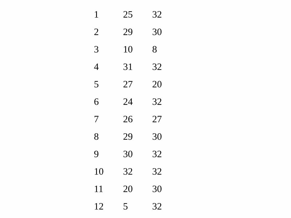
1 25 32
2 29 30
3 10 8
4 31 32
5 27 20
6 24 32
7 26 27
8 29 30
9 30 32
10 32 32
11 20 30
12 5 32

Wilcoxon Signed-Rank Test
Use the Wilcoxon matched-pair signed-rank test
to determine if the R&D expenses as a percent of income
(EXAMPLE 1) have declined.
Use the .05 significance level
Step 1: H0: Expenditure same in two years
H1: Expenditure not same in two years
Step 2: H0 is rejected if the smaller of the rank
sums is greater than or equal critical value
ontinued…

Company 2000 2001 Difference ABS-Diff Rank R+ R-
Savoth Glass 20 16 4 4
Ruisi Glass 14 13 1 1
Rubin Inc.. 23 20 3 3
Vaught 24 17 7 7
Lambert Glass 31 22 9 9
Pimental 22 20 2 2
Olson Glass 14 20 - 6 6
Flynn Glass 18 11 7 7
ontinued…
Wilcoxon Signed-Rank Test

The smaller rank sum is….., which is ……..than
critical value of T.
Company 2000 2001 Difference ABS-Diff Rank R+ R-
Savoth Glass 20 16 4 4
Ruisi Glass 14 13 1 1
Rubin Inc.. 23 20 3 3
Vaught 24 17 7 7
Lambert Glass 31 22 9 9
Pimental 22 20 2 2
Olson Glass 14 20 - 6 6
Flynn Glass 18 11 7 7
Wilcoxon Signed-Rank Test

The smaller rank sum is 5, which is greater to the
critical value of 3.
H0 can't be rejected
There is no evidence to say that expenditure is differ in two
years .
Company 2000 2001 Difference ABS-Diff Rank R+ R-
Savoth Glass 20 16 4 4 4 4 *
Ruisi Glass 14 13 1 1 1 1 *
Rubin Inc.. 23 20 3 3 3 3 *
Vaught 24 17 7 7 6.5 6.5 *
Lambert Glass 31 22 9 9 8 8 *
Pimental 22 20 2 2 2 2 *
Olson Glass 14 20 - 6 6 5 * 5
Flynn Glass 18 11 7 7 6.5 6 .5 *
Wilcoxon Signed-Rank Test

Example
Let Xi denote the length, in centimeters, of a
randomly selected pygmy sunfish, i = 1, 2, ...
10. If we obtain the following data set:
5.0 3.9 5.2 5.5 2.8
6.1 6.4 2.6 1.7 4.3
can we conclude that the median length of
pygmy sunfish differs significantly from 3.7
centimeters?
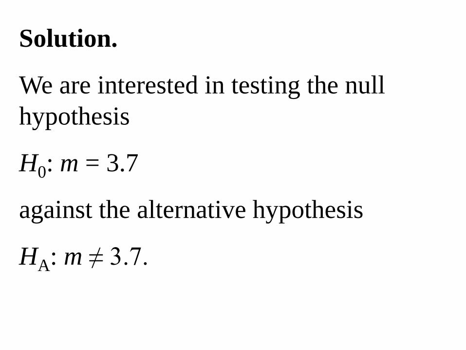
Solution.
We are interested in testing the null
hypothesis
H0: m = 3.7
against the alternative hypothesis
HA: m ≠ 3.7.


Solution. Recall that we are interested in testing
the null hypothesis H0: m = 3.7 against the
alternative hypothesis HA: m ≠ 3.7.
W = 15 (smaller value) for the given data set.
Tabulated value = 8
Tabulated value<calculated value
Can’t Reject H0

we cannot reject the null hypothesis.
There is no evidence at the 0.05 level to
conclude that the median length of
pygmy sunfish differs significantly
from 3.7 centimeters.

Normal Approximation when Sample
size is > 30
Wilcoxon Signed-Rank Test
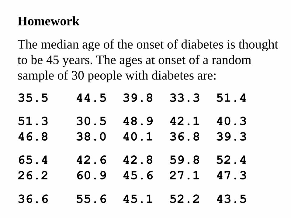
Homework
The median age of the onset of diabetes is thought
to be 45 years. The ages at onset of a random
sample of 30 people with diabetes are:
35.5 44.5 39.8 33.3 51.4
51.3 30.5 48.9 42.1 40.3
46.8 38.0 40.1 36.8 39.3
65.4 42.6 42.8 59.8 52.4
26.2 60.9 45.6 27.1 47.3
36.6 55.6 45.1 52.2 43.5

Solution. We are interested in testing the null
hypothesis
H0: m = 45
against the alternative hypothesis
HA: m ≠ 45.

Comparing Two Populations:Independent Samples

Mann-Whitney U test
• Tests two independent population probability distributions
• Corresponds to t-test for two independent means
• Assumptions
— Independent, random samples
— Populations are continuous
• Can use normal approximation if ni 10

Mann-Whitney test, step-by-step:
Does it make any difference to students'
comprehension of statistics whether the lectures
are in Theory base or in practical base?
Group 1: statistics lectures in Theory base.
Group 2: statistics lectures in Practical base.

theory group
(raw scores)
Practical group
(raw scores)
18 17
15 13
17 12
13 16
11 10
16 15
10 11
17 13
12

Step 1:
• Rank all the scores together, regardless of group
Step 2:
• Add up the ranks for group 1, to get R1.
• Add up the ranks for group 2, to get R2.
Step 3:
• n1 is the number of subjects in group 1; n2 is the number
of subjects in group 2. Here, n1 = 8 and n2 = 9.

Mann-Whitney U: CalculationStep 4:
Calculate two versions of the U statistic using:
U1 = (n1 x n2) + 2
(n1 + 1) x n1- ∑R1
AND…
U2 = (n1 x n2) + 2
(n2 + 1) x n2- ∑R2

Mann-Whitney U: Calculation
Calculate two versions of the U statistic using:
U1 = (n1 x n2) + 2
(n1 + 1) x n1- ∑R1
…OR to save time you can calculate U1 and then U2 as follows
U2 = (n1x n2) - U1

Mann-Whitney U: CalculationStep 5:
Select the smaller of the two U statistics (U1 & U2)
now consult a table of critical values for the
Mann-Whitney test
Calculated U must be less than critical U to
conclude a significant difference
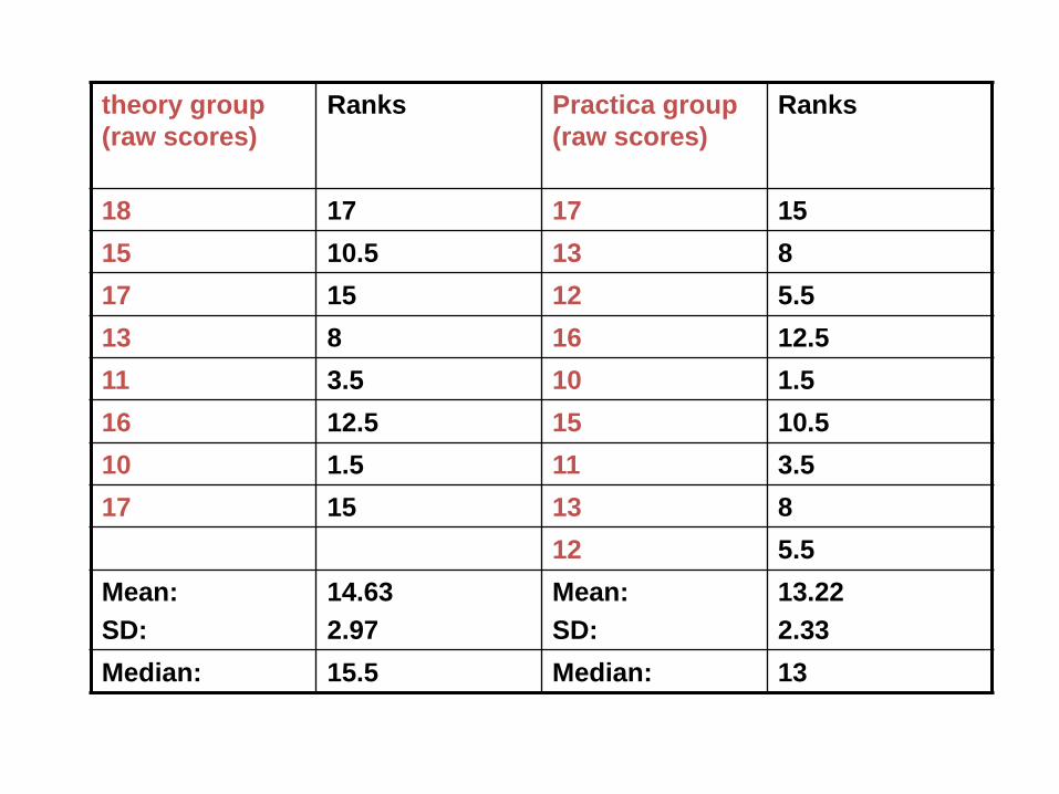
theory group
(raw scores)
Ranks Practica group
(raw scores)
Ranks
18 17 17 15
15 10.5 13 8
17 15 12 5.5
13 8 16 12.5
11 3.5 10 1.5
16 12.5 15 10.5
10 1.5 11 3.5
17 15 13 8
12 5.5
Mean:
SD:
14.63
2.97
Mean:
SD:
13.22
2.33
Median: 15.5 Median: 13
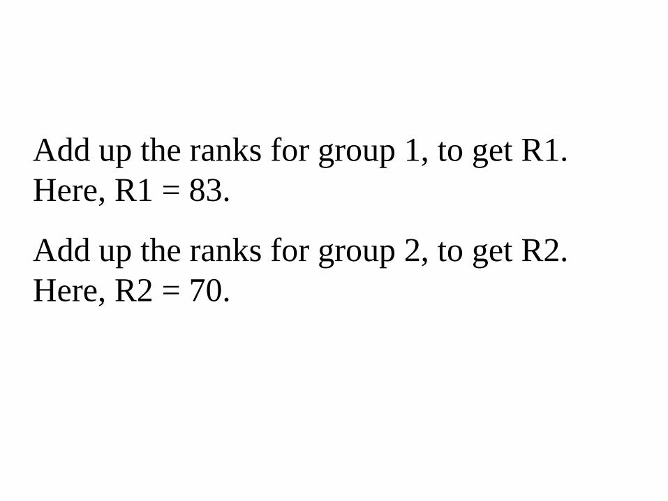
Add up the ranks for group 1, to get R1.
Here, R1 = 83.
Add up the ranks for group 2, to get R2.
Here, R2 = 70.

In the present example, U1 = 25, and, U2 =
47
Therefore, use 25 as U.

Here, the critical value of U for N1 = 8 and N2 = 9 is 15.
Our obtained U of 25 is larger than this, and so we cant
reject the Ho (Null hypothesis)
Conclusion: There is no evidence to say that Students
score for statistics is depend on the teaching methods.
N 2
N 1 5 6 7 8
2 3 5 6 7 8
3 5 6 8 10 11
5 6 8 10 12 14
6 8 10 13 15 17
7 10 12 15 17 20
8 11 14 17 20 23
9
10
5
6
7
8
9 10
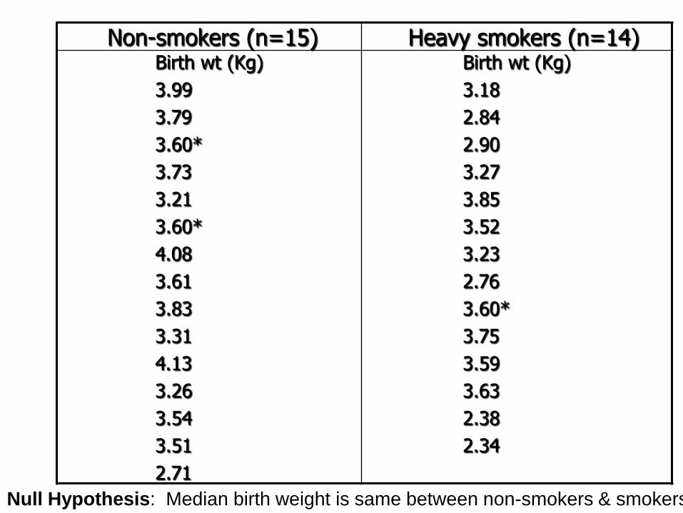
Non-smokers (n=15) Heavy smokers (n=14)Birth wt (Kg)
3.99
3.79
3.60*
3.73
3.21
3.60*
4.08
3.61
3.83
3.31
4.13
3.26
3.54
3.51
2.71
Birth wt (Kg)
3.18
2.84
2.90
3.27
3.85
3.52
3.23
2.76
3.60*
3.75
3.59
3.63
2.38
2.34
Null Hypothesis: Median birth weight is same between non-smokers & smokers

Non-smokers (n=15) Heavy smokers (n=14)Birth wt (Kg) Rank Birth wt (Kg) Rank
3.99 27 3.18 73.79 24 2.84 53.60* 18 2.90 63.73 22 3.27 113.21 8 3.85 263.60* 18 3.52 14
4.08 28 3.23 9
3.61 20 2.76 4
3.83 25 3.60* 183.31 12 3.75 234.13 29 3.59 163.26 10 3.63 213.54 15 2.38 23.51 13 2.34 12.71 3
Sum=272 Sum=163
* 17, 18 & 19are tied hence the ranks are
averaged

Hence calculated value of T = ; tabulated value of T
(14,15) =
median birth weights are not same for non-
smokers & smokers
they are significantly different

Mann-Whitney U testLarge-sample approximation:
Use this when n1& n2 are both > 10
Compare to the standard normal distribution
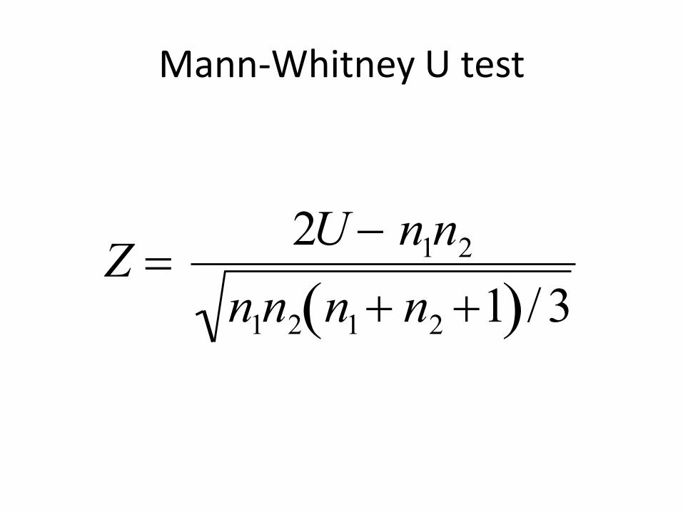
Mann-Whitney U test
Z 2U n1n2
n1n2 n1 n2 1 / 3

• The Kruskal-Wallis H Test is a nonparametric procedure that can be used to compare more than two populations in a completely randomized design.
• All n = n1+n2+…+nk measurements are jointly ranked (i.e. treat as one large sample).
• We use the sums of the ranks of the k samples to compare the distributions.
The Kruskal-Wallis H Test

Rank the total measurements in all k samples
from 1 to n. Tied observations are assigned average of
the ranks they would have gotten if not tied.
Calculate
Ti = rank sum for the ith sample i = 1, 2,…,k
And the test statistic
The Kruskal-Wallis H Test
)1(3)1(
12 2
nn
T
nnH
i
i

H0: the k distributions are identical versus
Ha: at least one distribution is different
Test statistic: Kruskal-Wallis H
When H0 is true, the test statistic H has an
approximate chi-square distribution with df
= k-1.
Use a right-tailed rejection region or p-
value based on the Chi-square distribution.
The Kruskal-Wallis H Test

Example
Four groups of students were randomly
assigned to be taught with four different
techniques, and their achievement test scores
were recorded. Are the distributions of test
scores the same, or do they differ in location?
88628179
67
78
59
3
83
69
75
2
73
87
65
1
80
89
94
4
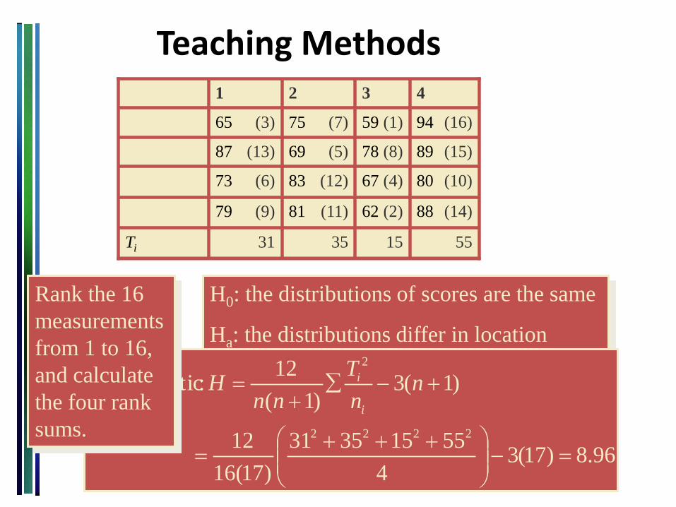
Teaching Methods
H0: the distributions of scores are the same
Ha: the distributions differ in location
88628179
67
78
59
3
83
69
75
2
73
87
65
1
80
89
94
4
55153531Ti
(14)(2)(11)(9)
(4)
(8)
(1)
(12)
(5)
(7)
(6)
(13)
(3)
(10)
(15)
(16)
96.8)17(34
55153531
)17(16
12
)1(3)1(
12
2222
2
nn
T
nnH
i
i :statistic Test
Rank the 16
measurements
from 1 to 16,
and calculate
the four rank
sums.

Teaching MethodsH0: the distributions of scores are the same
Ha: the distributions differ in location
96.8)17(34
55153531
)17(16
12
)1(3)1(
12
2222
2
nn
T
nnH
i
i :statistic Test
Rejection region: For a right-
tailed chi-square test with =
.05 and df = 4-1 =3, reject H0 if
H 7.81.
Reject H0. There is sufficient
evidence to indicate that there
is a difference in test scores for
the four teaching techniques.

Kruskal-Wallis test Class example
Does it make any difference to students’ comprehension of
statistics whether the lectures are given in teacher centred,
student centred or self study?
Group A: teacher centred;
Group B: Student centred ;
Group C: Self study
DV: student rating of lecturer's intelligibility on 100-point
scale ("0" = "incomprehensible").
Ratings - so use a nonparametric test.

Group A
(raw score)
Group B
(raw score)
Group C
(raw score)
20 25 19
27 33 20
19 35 25
23 36 22

Group A
(raw score)
(rank) Group B
(raw score)
(rank) Group C
(raw score) (rank)
20 3.5 25 7.5 19 1.5
27 9 33 10 20 3.5
19 1.5 35 11 25 7.5
23 6 36 12 22 5
M = 22.25
SD = 3.59
M = 32.25
SD = 4.99
M = 21.50
SD = 2.65

Tc1 (the total for the 1st group) is 20.
Tc2 (for the 2nd group) is 40.5.
Tc3 (for the 3rd group) is 17.5.

)1(3)1(
12 2
nn
T
nnH
i
i

12.613362.58613*12
12
62.5864
5.17
4
5.40
4
202222
H
n
Tc
c
)(

Degrees of freedom are the number of groups minus one. Here, d.f. = 3 - 1 = 2.
Assessing the significance of H depends on the number of participants and the
number of groups.
(a) If you have 3 groups and N in each group is 5 or less:
Special tables exist for small sample sizes – but you really should run more
participants!
(b) If N in each group is larger than 5:
Treat H as Chi-Square.
H is statistically significant if it is larger than the critical value of Chi-Square for
these d.f.
For 2 d.f., a Chi-Square of 5.99 has a p = .05 of occurring by chance.
Our H is bigger than 5.692, and so even less likely to occur by chance!

Conclusion:
The three groups differ significantly;

Table of Chi-square p
n 0.99 0.95 0.50 0.30 0.20 0.10 0.05 0.01
1 0.0002 0.004 0.46 1.07 1.64 2.71 3.84 6.64
2 0.020 0.103 1.39 2.41 3.22 4.00 5.99 9.21
3 0.115 0.35 2.17 3.66 4.64 6.25 7.82 11.34
4 0.30 0.71 3.86 4.88 5.99 7.78 9.49 13.28
5 0.55 1.14 4.35 6.06 7.29 9.24 11.07 15.09
6 0.87 1.64 5.35 7.23 8.56 10.64 12.59 16.81
7 1.24 2.17 6.35 8.38 9.80 12.02 14.07 18.48
8 1.65 2.73 7.34 9.52 11.03 13.36 15.51 20.09
9 2.09 3.32 8.34 10.66 12.24 14.68 16.92 21.67
10 2.56 3.94 9.34 11. 78 13.44 15.99 18.31 23.21
11 3.05 4.58 10.34 12.90 14.63 17.28 19.68 24.72
12 3.37 5.23 11.34 14.01 15.81 18.55 21.03 26.22
13 4.11 5.89 12.34 15.12 16.98 19.81 22.36 27.69
14 4;66 6.57 13.34 16.22 18.15 21.06 23.68 29.14
15 5.23 7.26 14.34 17.32 19.31 22.31 25.00 30.58
16 5.81 7.96 15.34 18.42 20.46 23.54 26.30 32.06
17 6.41 8.67 16.34 19.51. 21.62 24.77 27.59 33.41
18 7.02 9.39 17.34 20.60 22.76 25.99 28.87 34.80
19 7.63 10.12 18.34 21.69 23.90 27.20 30.14 36.19
20 8.26 10.85 19.34 22.78 25.04 28.41 31.41 37.57

Friedman’s test
Effects on worker mood of different types of
music:
Five workers. Each is tested three times, once
under each of the following conditions:
condition 1: silence.
condition 2: "easy-listening‖ music.
condition 3: marching-band music.
DV: mood rating ("0" = unhappy, "10" = very
happy).
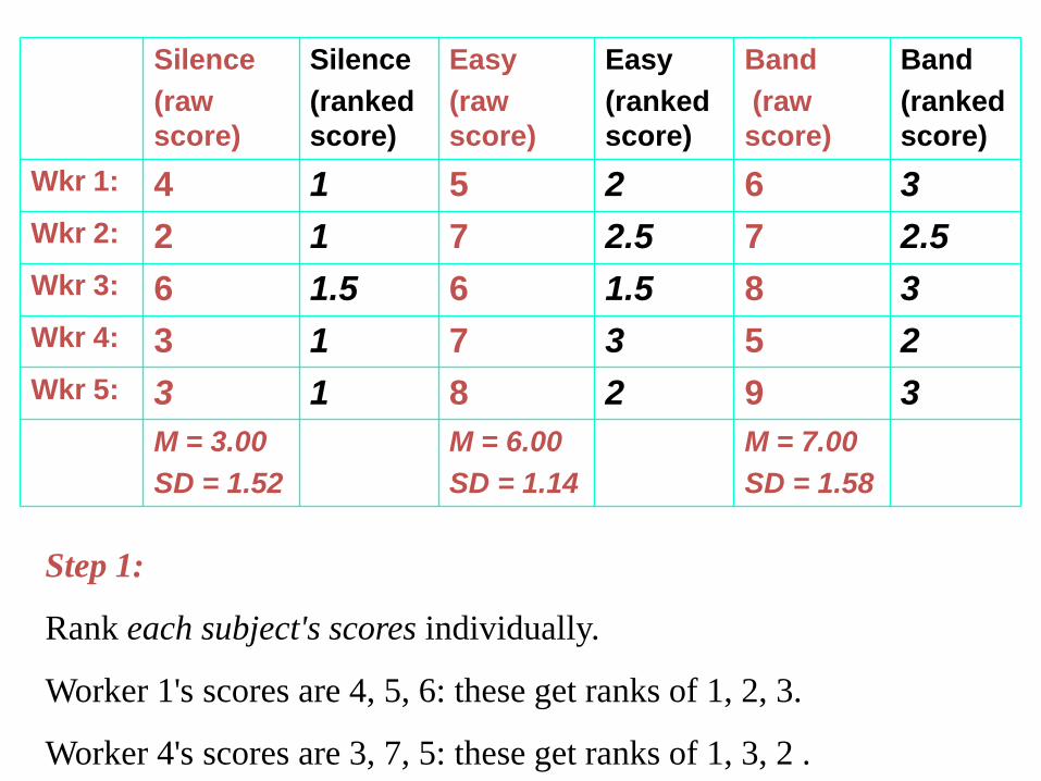
Step 1:
Rank each subject's scores individually.
Worker 1's scores are 4, 5, 6: these get ranks of 1, 2, 3.
Worker 4's scores are 3, 7, 5: these get ranks of 1, 3, 2 .
Silence
(raw
score)
Silence
(ranked
score)
Easy
(raw
score)
Easy
(ranked
score)
Band
(raw
score)
Band
(ranked
score)
Wkr 1: 4 1 5 2 6 3
Wkr 2: 2 1 7 2.5 7 2.5
Wkr 3: 6 1.5 6 1.5 8 3
Wkr 4: 3 1 7 3 5 2
Wkr 5: 3 1 8 2 9 3
M = 3.00
SD = 1.52
M = 6.00
SD = 1.14
M = 7.00
SD = 1.58

Silence
(raw
score)
Silence
(ranked
score)
Easy
(raw
score)
Easy
(ranked
score)
Band
(raw
score)
Band
(ranked
score)
Wkr 1: 4 1 5 2 6 3
Wkr 2: 2 1 7 2.5 7 2.5
Wkr 3: 6 1.5 6 1.5 8 3
Wkr 4: 3 1 7 3 5 2
Wkr 5: 3 1 8 2 9 3
rank
total:5.5 11 13.5

Step 2:
Find the rank total for each condition, using the ranks
from all subjects within that condition.
Rank total for ‖Silence" condition: 1+1+1.5+1+1 = 5.5.
Rank total for ―Easy Listening‖ condition = 11.
Rank total for ―Marching Band‖ condition = 13.5.

Step 3: Work out r2
13
1
12 22
CNTc
CCNr
C is the number of conditions.
N is the number of subjects.
Tc2 is the sum of the squared rank totals
for each condition.

To get Tc2 :
(a) square each rank total:
5.52 = 30.25. 112 = 121. 13.52 = 182.25.
(b) Add together these squared totals.
30.25 + 121 + 182.25 = 333.5.
13
1
12 22
CNTc
CCNr
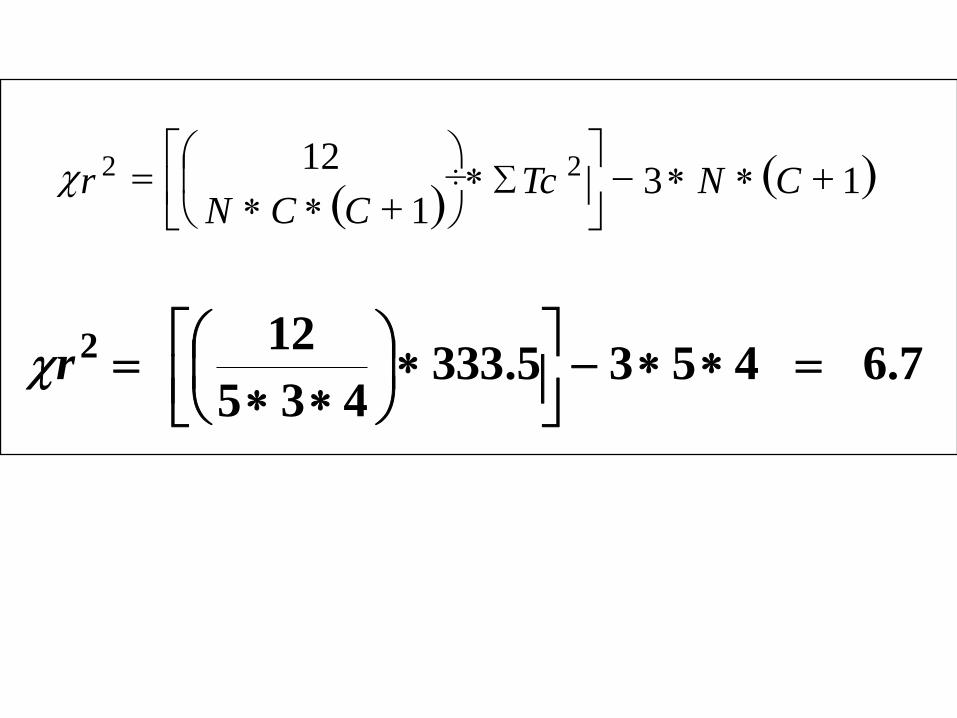
7.64535.333435
122
r
13
1
12 22
÷
CNTc
CCNr

Step 5:
Assessing the statistical significance of r2 depends
on the number of participants and the number of
groups.
r2 = 6.7
Step 4:
Degrees of freedom = number of conditions minus
one. df = 3 - 1 = 2.
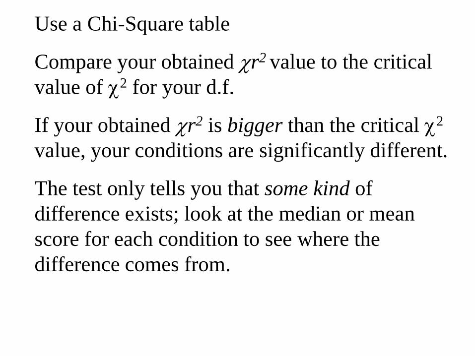
Use a Chi-Square table
Compare your obtained r2 value to the critical
value of 2 for your d.f.
If your obtained r2 is bigger than the critical 2
value, your conditions are significantly different.
The test only tells you that some kind of
difference exists; look at the median or mean
score for each condition to see where the
difference comes from.
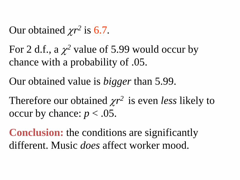
Our obtained r2 is 6.7.
For 2 d.f., a 2 value of 5.99 would occur by
chance with a probability of .05.
Our obtained value is bigger than 5.99.
Therefore our obtained r2 is even less likely to
occur by chance: p < .05.
Conclusion: the conditions are significantly
different. Music does affect worker mood.

Term Description
j 1, 2, ..., k
k the number of treatment conditions
n the number of blocks
Rj the sum of ranks for treatment j
i 1, 2, ..., m
m the number of sets of ties
ti the number of tied scores in the ithset of ties
If the data have ties, the formula is:
where C is a correction factor that is equal to:
Notation

Exercise: Friedman Test
Six judges with different expertise were asked to
rank 5 different types of ready to drink milk
packets from 1 to 10, where 10 represents a most
prefer. The data were given in the table. Can you
select a best drink according to the rank given by
the judges.

Judge A B C D E1 3.9 4.1 4.2 4.1 3.32 9.4 9.5 9.4 9.0 8.63 9.7 9.3 9.3 9.2 8.44 8.3 8.0 7.9 8.6 7.45 9.8 8.9 9.0 9.0 8.36 9.9 10.0 9.7 9.6 9.1

Rank-Order Correlation
…Spearman’s coefficient of rank correlation reports the
association between two sets of ranked observations
Features
…it can range from –1.00 up to 1.00
…it is similar to Pearson’s coefficient of
correlation, but is based on ranked data
ontinued…

Spearman’s
Rank-Order Correlation
Formula (to find the coefficient of rank correlation)
d is the difference in the ranks and n is the number of
observations.
rd
n ns
1
6
1
2
2
( )
ontinued…

Spearman’s
Rank-Order Correlation
Testing the significance of rs
State the null hypothesis:
Rank correlation in population is 0
State the alternate hypothesis:
Rank correlation in population is not 0.
The value of the test statistic is computed from …
t rs
n
rs2
2
1
Spearman’s
Rank-Order Correlation
The preseason football rankings for the Atlantic Coast Conference
by the coaches and sports writers are shown below. What is the
coefficient of rank correlation between the two groups?

School Coaches Writers
Maryland 2 3
NC State 3 4
NC 6 6
Virginia 5 5
Clemson 4 2
Wake Forest 7 8
Duke 8 7
Florida State 1 1

School Coaches Writers d d2
Maryland 2 3 -1 1
NC State 3 4 -1 1
NC 6 6 0 0
Virginia 5 5 0 0
Clemson 4 2 2 4
Wake Forest 7 8 -1 1
Duke 8 7 1 1
Florida State 1 1 0 0

= 0.905)18(8
)8(61
2
)1(
61
2
2
nn
drs
There is a strong correlation between the ranks of the coaches and
the sports writers!

The hypothesis tested is that prices should decrease with
distance from the key area of surrounding the Contemporary Art
Museum. Following data are from continuous sampling of the
price of a 50ml bottle water at every convenience store.
Convenience
Store
Distance from
CAM (m)
Price of 50ml
bottle (Rs)
1 50 28.0
2 175 22.0
3 270 30.0
4 375 20.0
5 425 20.0
6 580 22.0
7 710 18.0
8 790 16.0
9 890 20.0
10 980 18.5

Conveni
ence
Store
Distance
from CAM
(m)
Rank
distanc
e
Price of
50ml
bottle
(Rs)
Rank
price
Difference
between
ranks (d)
d²
1 50 10 28.0 2 8 64
2 175 9 22.0 3.5 5.5 30.25
3 270 8 30.0 1 7 49
4 375 7 20.0 6 1 1
5 425 6 20.0 6 0 0
6 580 5 22.0 3.5 1.5 2.25
7 710 4 18.0 9 -5 25
8 790 3 16.0 10 -7 49
9 890 2 20.0 6 -4 16
10 980 1 18.5 8 -7 49
d² = 285.5

![(eBook-PDF) - Statistics - Applied Nonparametric Regression[1]](https://cdn.vdocument.in/doc/165x107/55cf99ab550346d0339e92b5/ebook-pdf-statistics-applied-nonparametric-regression1.jpg)


