
Chapter 5Chapter 5
ChoiceChoice

Economic RationalityEconomic Rationality
The principal behavioral postulate is that a decisionmaker chooses itsthat a decisionmaker chooses its most preferred alternative from those available to itavailable to it.
The available choices constitute the choice set.
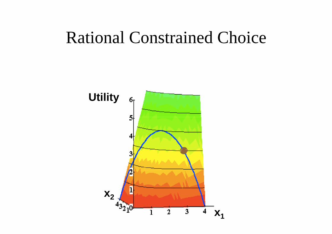
How is the most preferred bundle in How is the most preferred bundle in the choice set located?
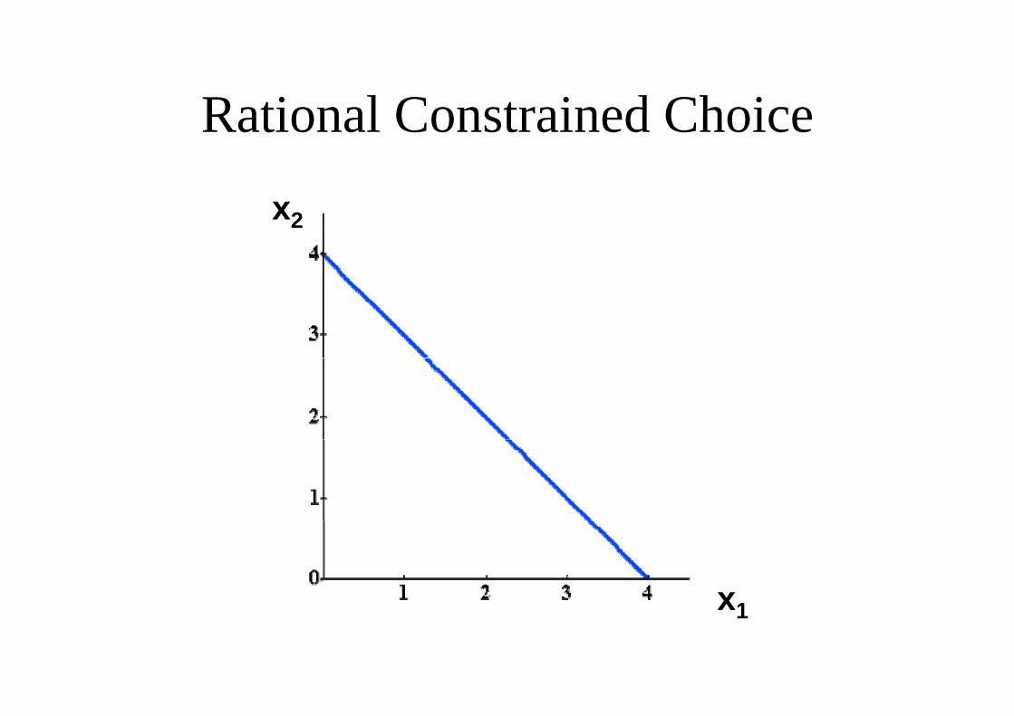
Rational Constrained ChoiceRational Constrained Choice
x2
xx1

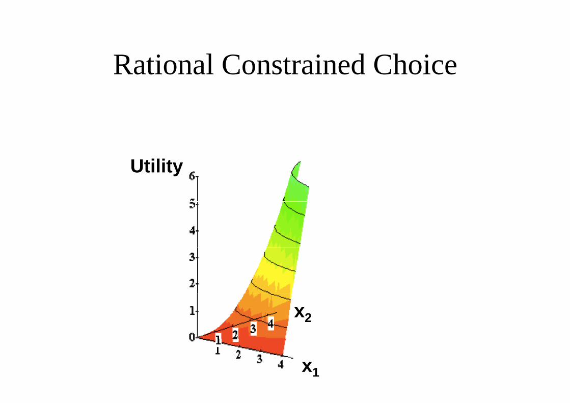
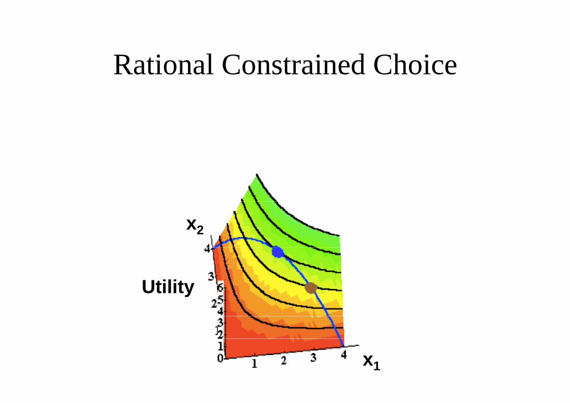
Rational Constrained ChoiceRational Constrained Choice
UtilitUtility
x1

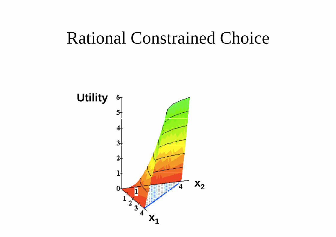
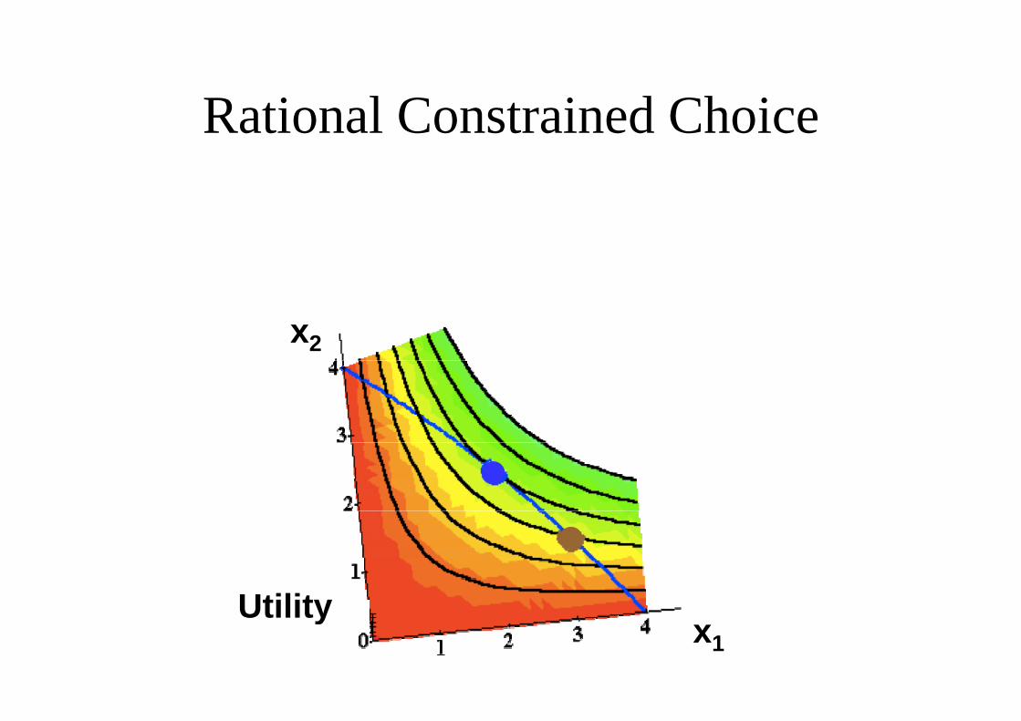
Rational Constrained ChoiceRational Constrained Choice
UtilitUtility x2
x1
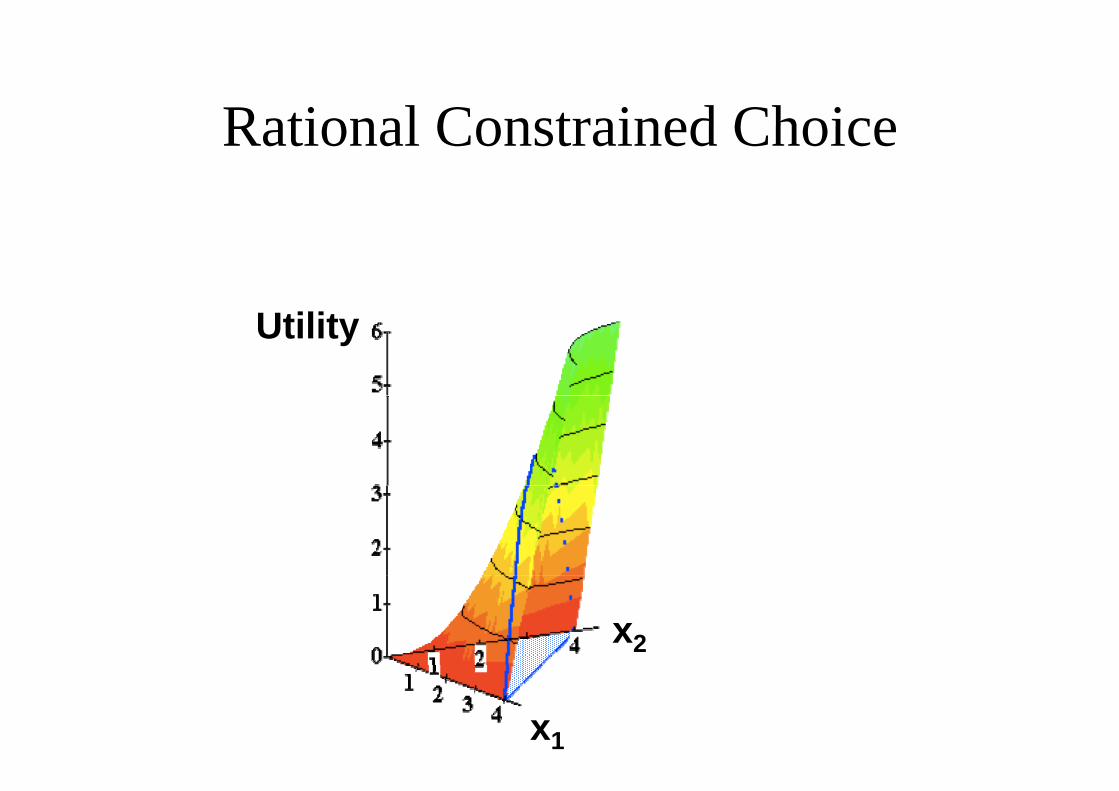
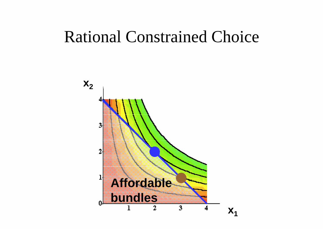
Rational Constrained ChoiceRational Constrained Choice
Utility
x2
x1
Rational Constrained ChoiceRational Constrained Choice
Utility
x2
x1
Rational Constrained ChoiceRational Constrained Choice
Utility
x2
x1

Rational Constrained ChoiceRational Constrained Choice
Utility
x2
x1
Rational Constrained ChoiceRational Constrained Choice
Utility
x2
x1
x2

Rational Constrained ChoiceRational Constrained Choice
Utility
Affordable, but not the most preferred affordable bundle.
x2
x1
x2

Rational Constrained ChoiceRational Constrained Choice
Utility The most preferredof the affordable
Affordable, but not bundles.
the most preferred affordable bundle.
x2
x1
x2

Rational Constrained ChoiceRational Constrained Choice
Utility
x2
x1
x2

Rational Constrained ChoiceRational Constrained Choice
Utility
x22
x1
Rational Constrained ChoiceRational Constrained Choice
x2
UtilityUtility
x1
Rational Constrained ChoiceRational Constrained Choice
x2
UtilityUtilityx1

Rational Constrained ChoiceRational Constrained Choice
x22
x1
Rational Constrained ChoiceRational Constrained Choice
x22
Affordable
x1
bundles

Rational Constrained ChoiceRational Constrained Choice
x22
Affordable
x1
bundles

Rational Constrained ChoiceRational Constrained Choice
x22
More preferredMore preferredbundles
Affordable
x1
bundles

Rational Constrained ChoiceRational Constrained Choicex2
More preferredbundles
Affordablebundles
xx1
Rational Constrained ChoiceRational Constrained Choicex2
x2*
xx * x1x1*
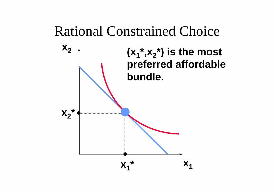
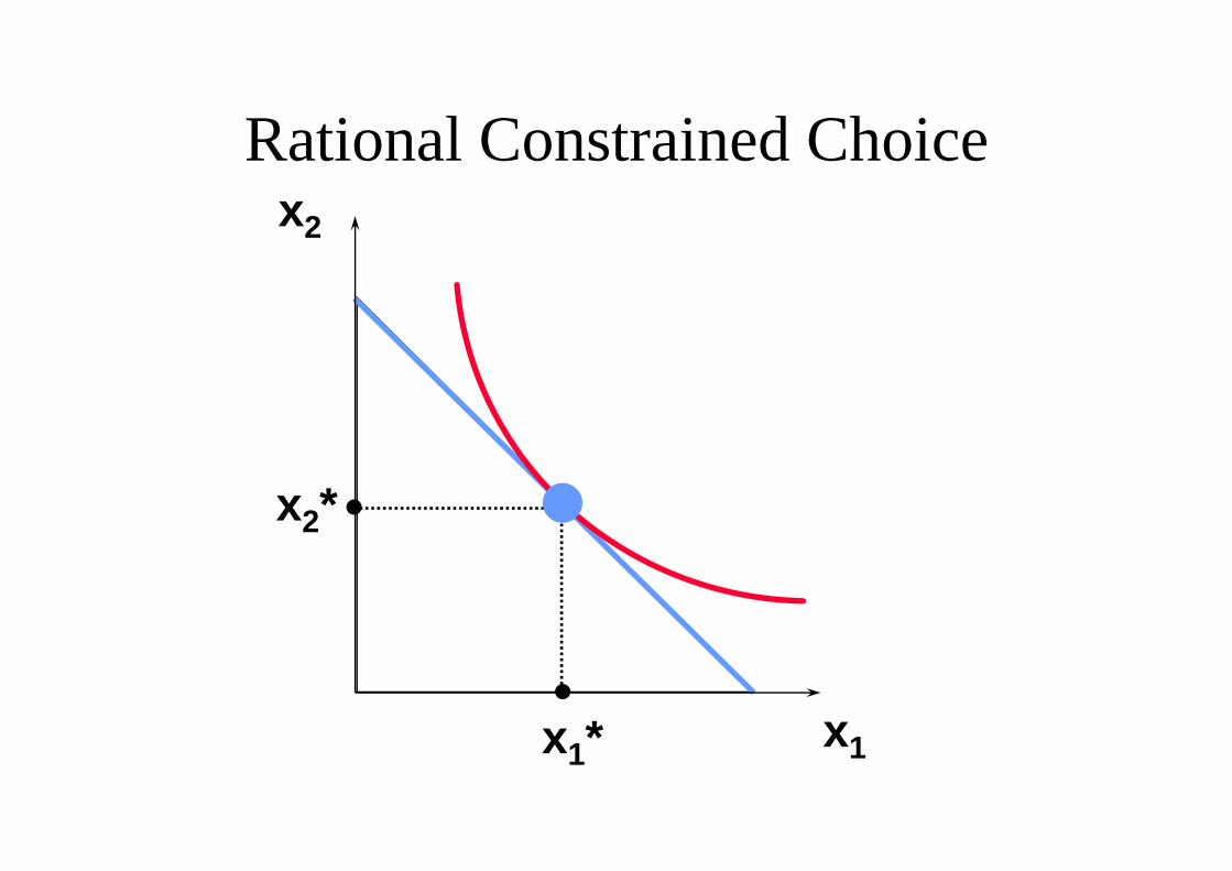
Rational Constrained ChoiceRational Constrained Choicex2 (x1* x2*) is the most(x1 ,x2 ) is the most
preferred affordablebundlebundle.
x2*
xx * x1x1*

Rational Constrained ChoiceRational Constrained Choice
The most preferred affordable bundle is called the consumer’s ORDINARYis called the consumer s ORDINARY DEMAND at the given prices and budgetbudget.
Ordinary demands will be denoted byy yx1*(p1,p2,m) and x2*(p1,p2,m).

Rational Constrained ChoiceRational Constrained Choice
When x1* > 0 and x2* > 0 the demanded bundle is INTERIORdemanded bundle is INTERIOR.
If buying (x1*,x2*) costs $m then the b d i h dbudget is exhausted.

Rational Constrained ChoiceRational Constrained Choicex2 (x1* x2*) is interior(x1 ,x2 ) is interior.
(x1*,x2*) exhausts thebudget.
x2*
g
xx * x1x1*
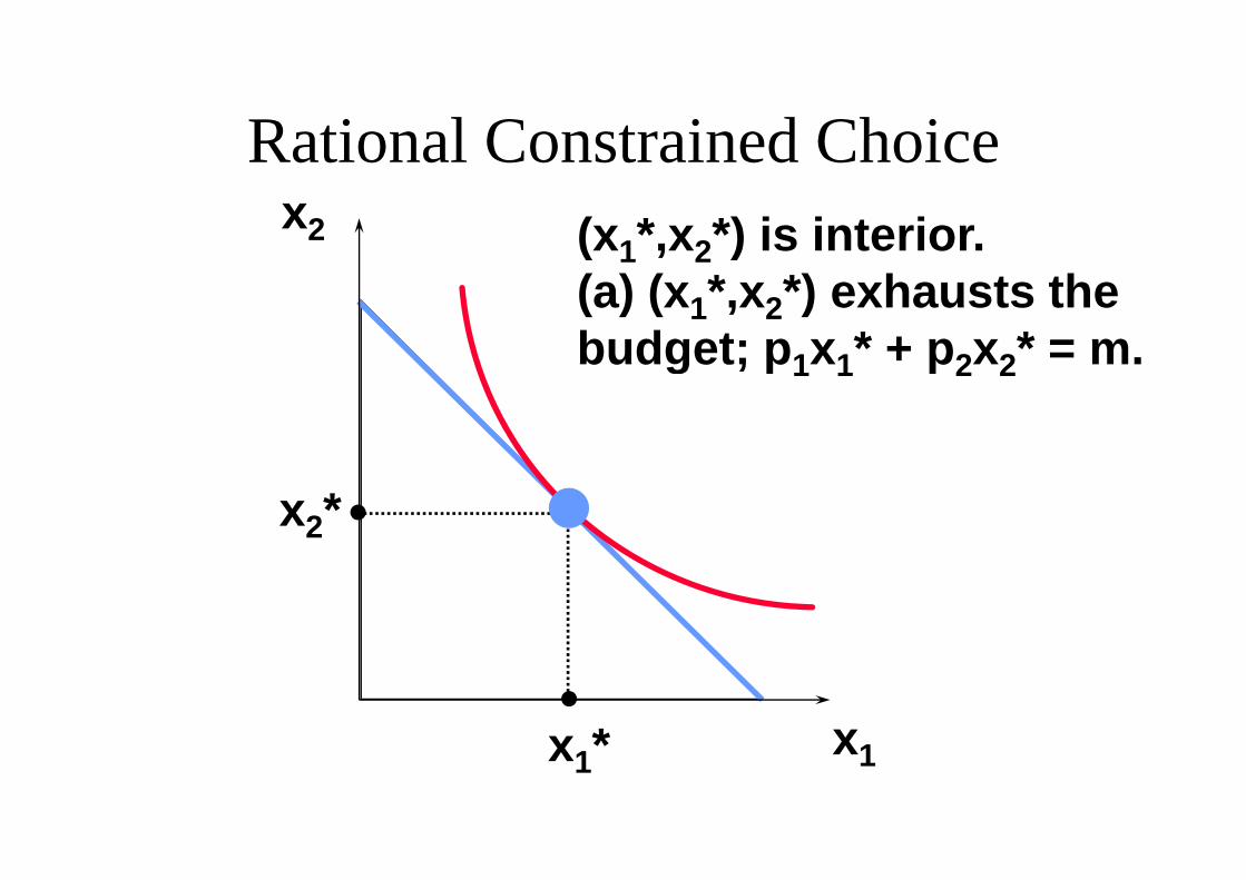
Rational Constrained ChoiceRational Constrained Choicex2 (x1* x2*) is interior(x1 ,x2 ) is interior.
(a) (x1*,x2*) exhausts thebudget; p x * + p x * = mbudget; p1x1* + p2x2* = m.
x2*
xx * x1x1*
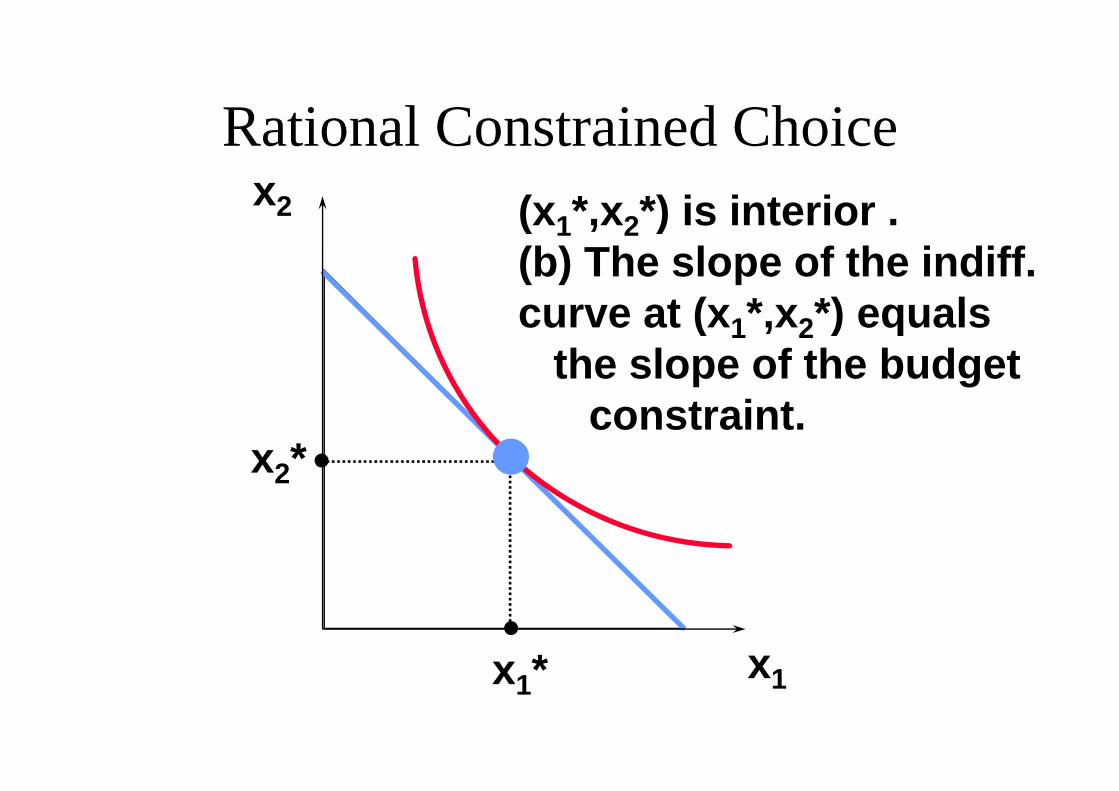
Rational Constrained ChoiceRational Constrained Choicex2 (x1* x2*) is interior(x1 ,x2 ) is interior .
(b) The slope of the indiff.curve at (x * x *) equalscurve at (x1*,x2*) equals
the slope of the budget
x2*constraint.
xx * x1x1*
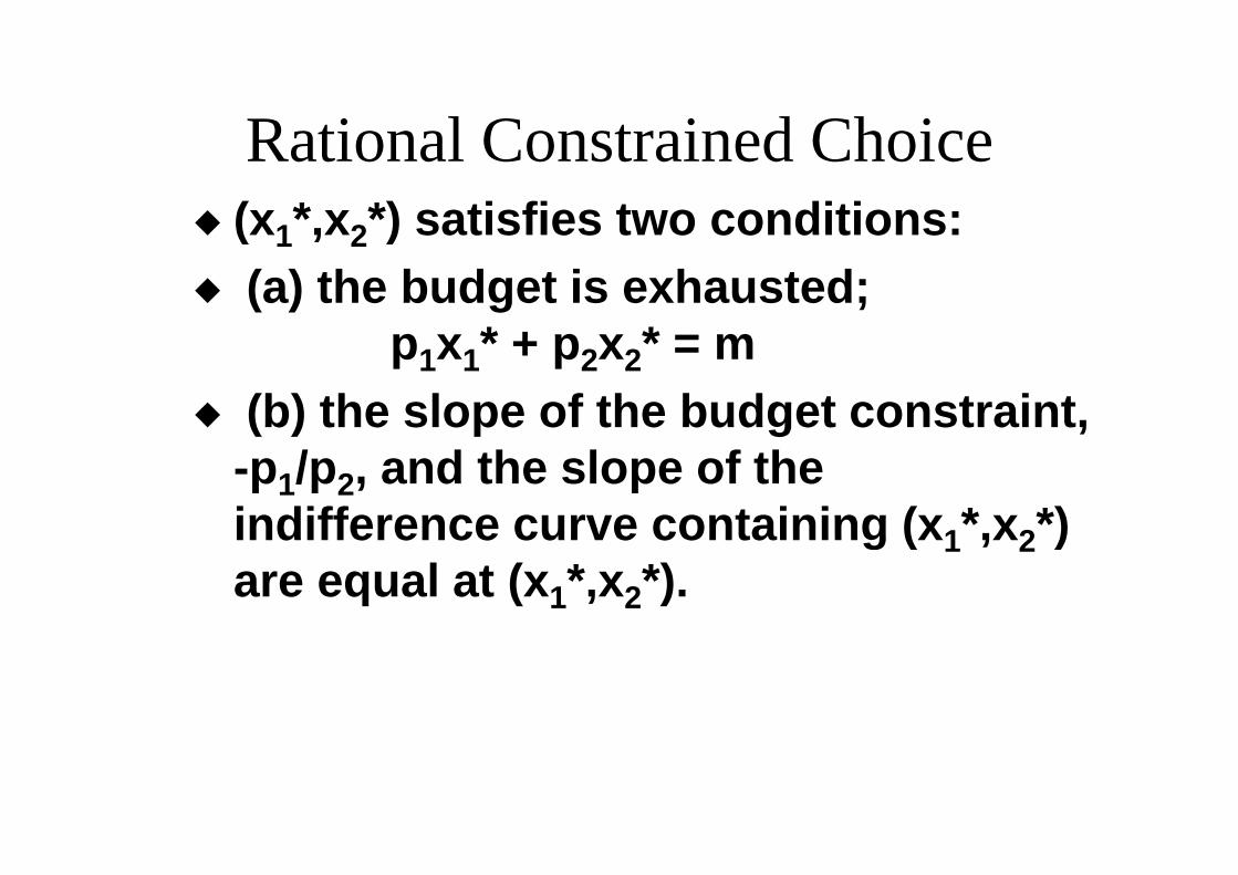
Rational Constrained ChoiceRational Constrained Choice (x1*,x2*) satisfies two conditions:( 1 , 2 ) (a) the budget is exhausted;
p x * + p x * = mp1x1* + p2x2* = m (b) the slope of the budget constraint,
-p1/p2, and the slope of the indifference curve containing (x1*,x2*)indifference curve containing (x1 ,x2 ) are equal at (x1*,x2*).
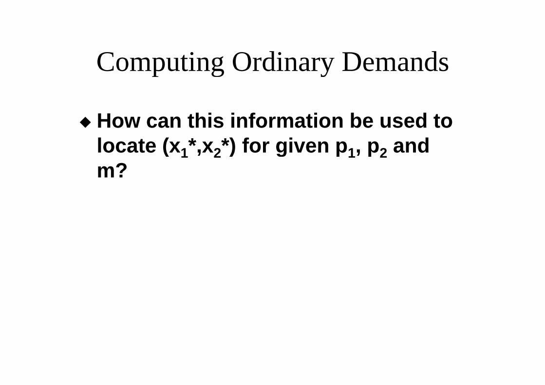
Computing Ordinary DemandsComputing Ordinary Demands
How can this information be used to locate (x1* x2*) for given p1 p2 andlocate (x1 ,x2 ) for given p1, p2 and m?

Computing Ordinary Demands -a Cobb-Douglas Example.
Suppose that the consumer has Cobb-Douglas preferencesCobb Douglas preferences.
U x x x xa b( , )1 2 1 2( , )1 2 1 2

Computing Ordinary Demands -a Cobb-Douglas Example.
Suppose that the consumer has Cobb-Douglas preferencesCobb Douglas preferences.
U x x x xa b( , )1 2 1 2
Then
( , )1 2 1 2
MU U ax xa b1 1
12
x11
1 2
UMU Ux
bx xa b2
21 2
1

Computing Ordinary Demands -a Cobb-Douglas Example.
So the MRS is
MRS dx U x ax x axa b
2 1 1
12 2 /MRS
dx U x bx x bxa b 1 2 1 21 1 /
.
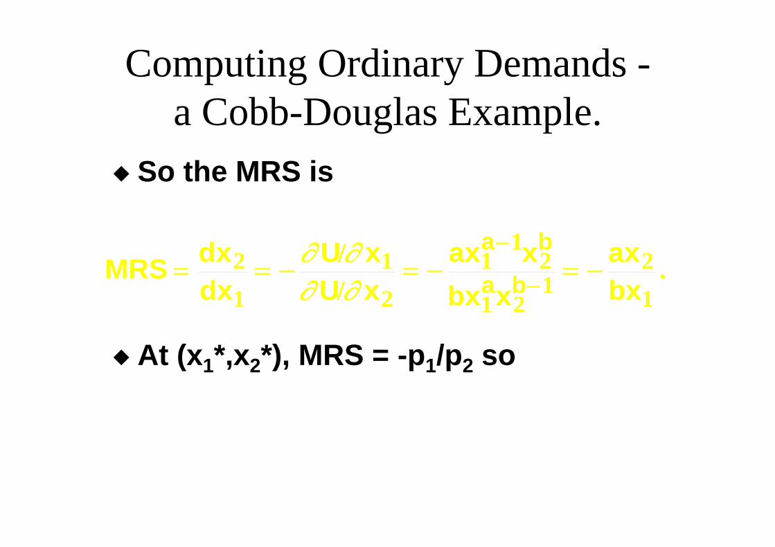
Computing Ordinary Demands -a Cobb-Douglas Example.
So the MRS is
MRS dx U x ax x axa b
2 1 1
12 2 /MRS
dx U x bx x bxa b 1 2 1 21 1 /
.
At (x1*,x2*), MRS = -p1/p2 so

Computing Ordinary Demands -a Cobb-Douglas Example.
So the MRS is
MRS dx U x ax x axa b
2 1 1
12 2 /MRS
dx U x bx x bxa b 1 2 1 21 1 /
.
At (x1*,x2*), MRS = -p1/p2 so
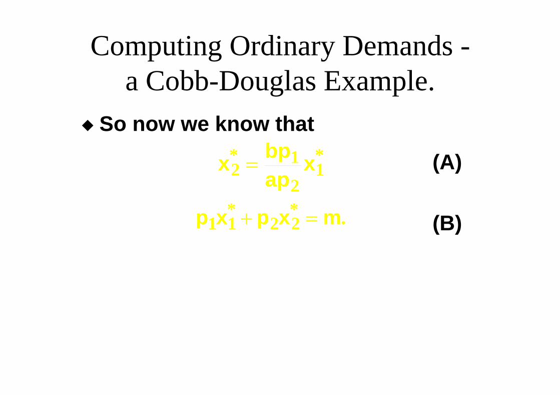
b* ax
bxpp
x bpap
x2
1
12
212
1** *. (A)
bx p p1 2 2
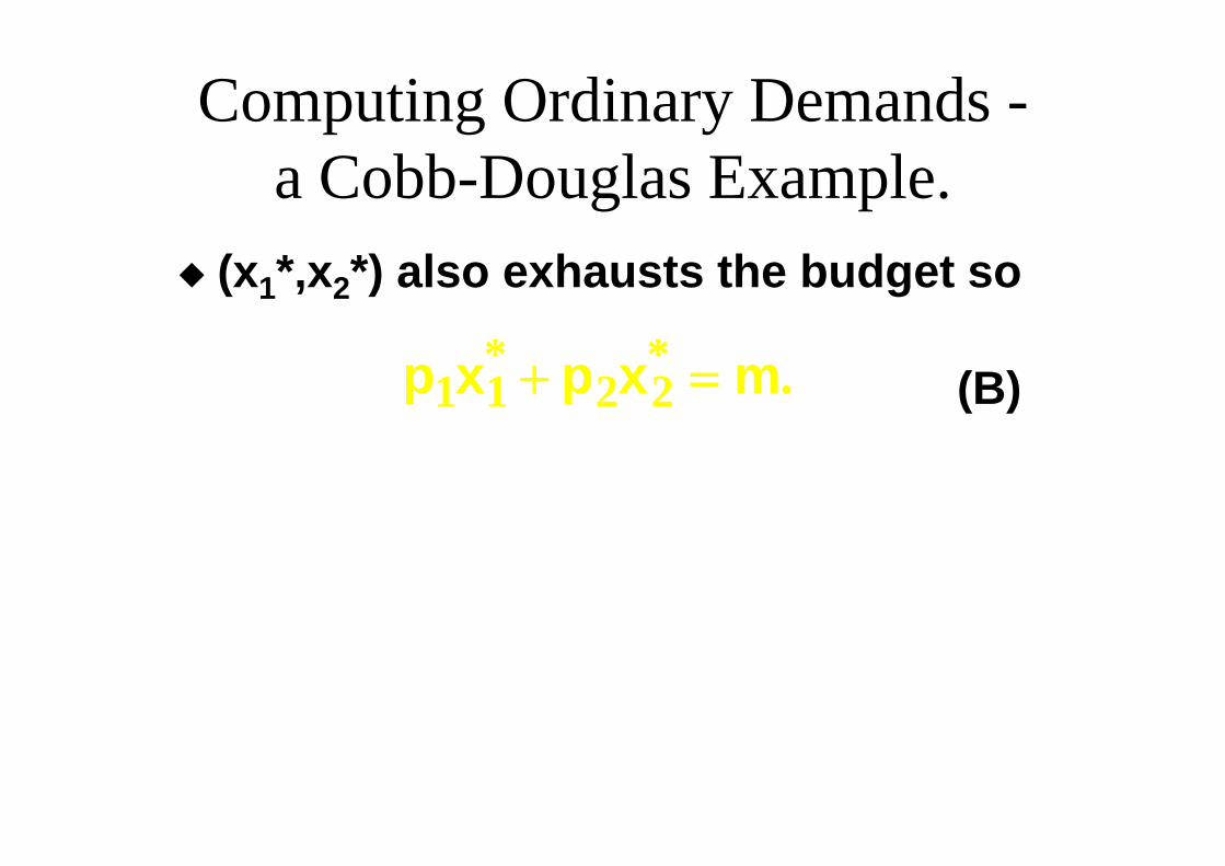
Computing Ordinary Demands -a Cobb-Douglas Example.
(x1*,x2*) also exhausts the budget so
p x p x m1 1 2 2* * . (B)
Computing Ordinary Demands -a Cobb-Douglas Example.
So now we know thatbp1* *x bpap
x212
1* * (A)
p x p x m1 1 2 2* * . (B)
Computing Ordinary Demands -a Cobb-Douglas Example.
So now we know thatbp1* *x bpap
x212
1* * (A)
Substitutep x p x m1 1 2 2
* * . (B)Substitute

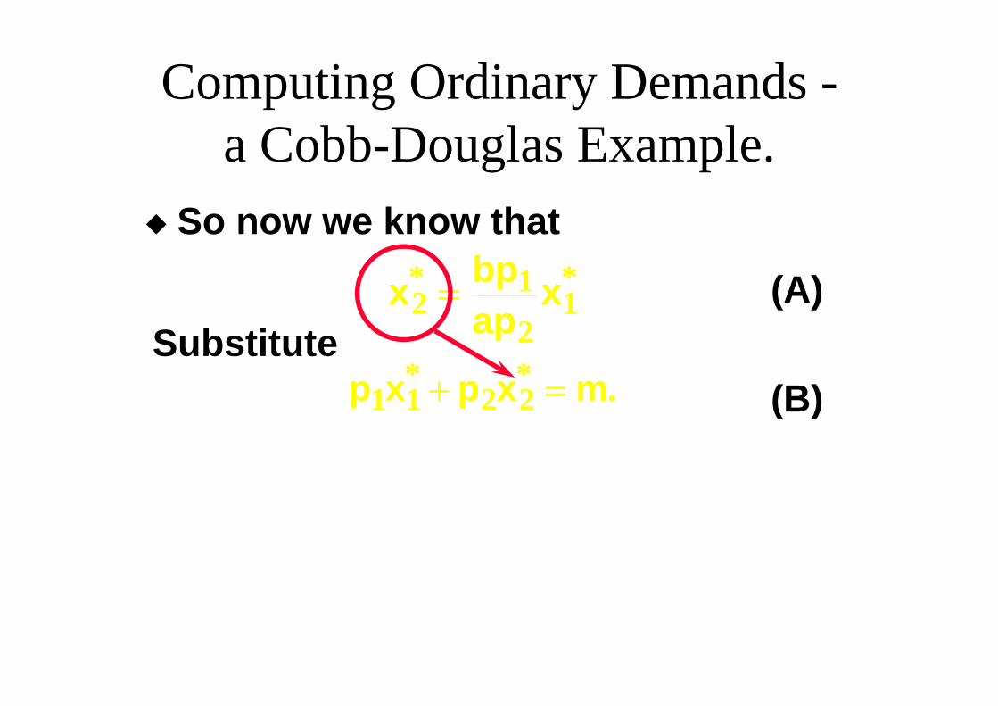
Computing Ordinary Demands -a Cobb-Douglas Example.
So now we know thatbp1* *x bpap
x212
1* * (A)
Substitutep x p x m1 1 2 2
* * . (B)Substitute
d tp x p bp
apx m1 1 2
11
* * . and get
ap2This simplifies to ….

Computing Ordinary Demands -a Cobb-Douglas Example.
x ama b p1
1
*( )
.a b p1( )
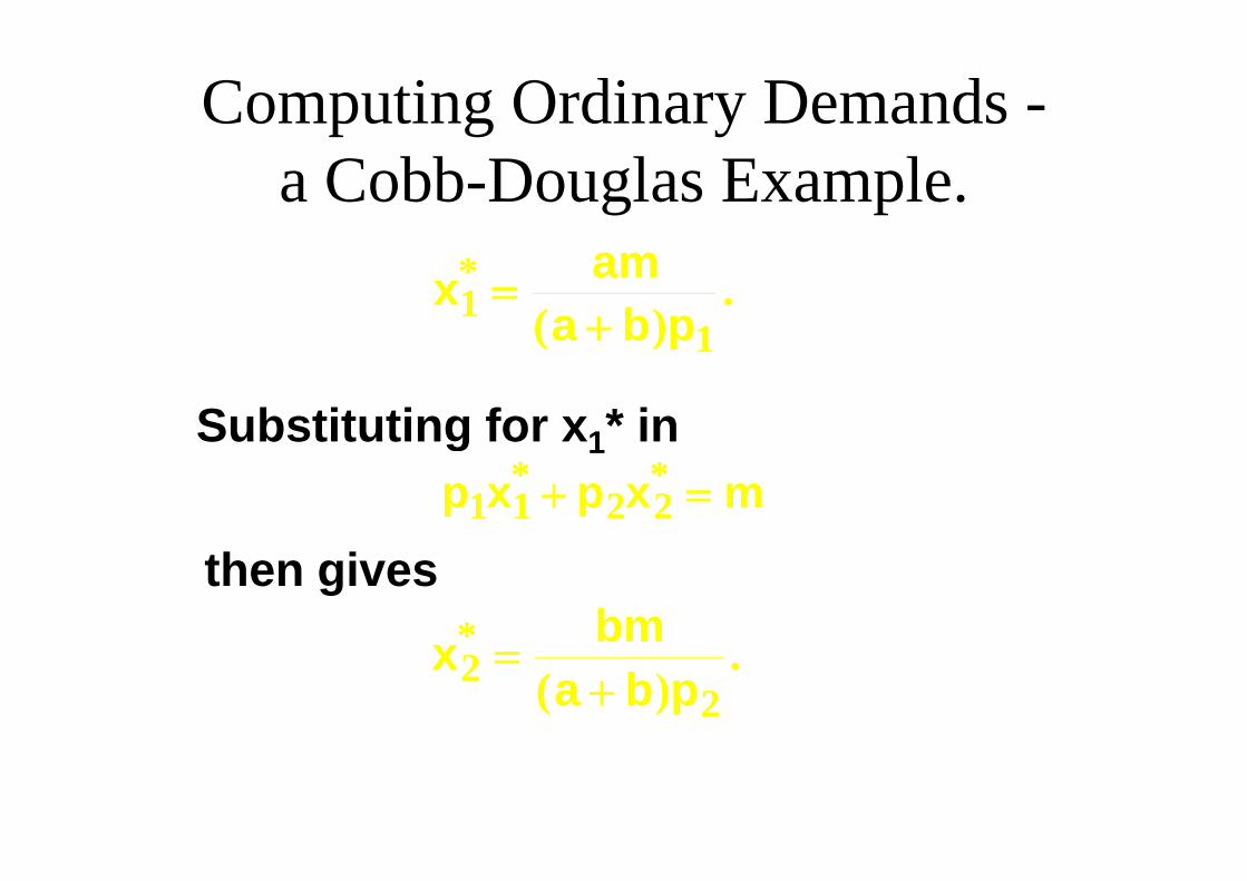
Computing Ordinary Demands -a Cobb-Douglas Example.
x ama b p1
1
*( )
.
Substituting for x1* in
a b p1( )
Substituting for x1 in p x p x m1 1 2 2
* *
bm*then gives
x bma b p2
2( ).
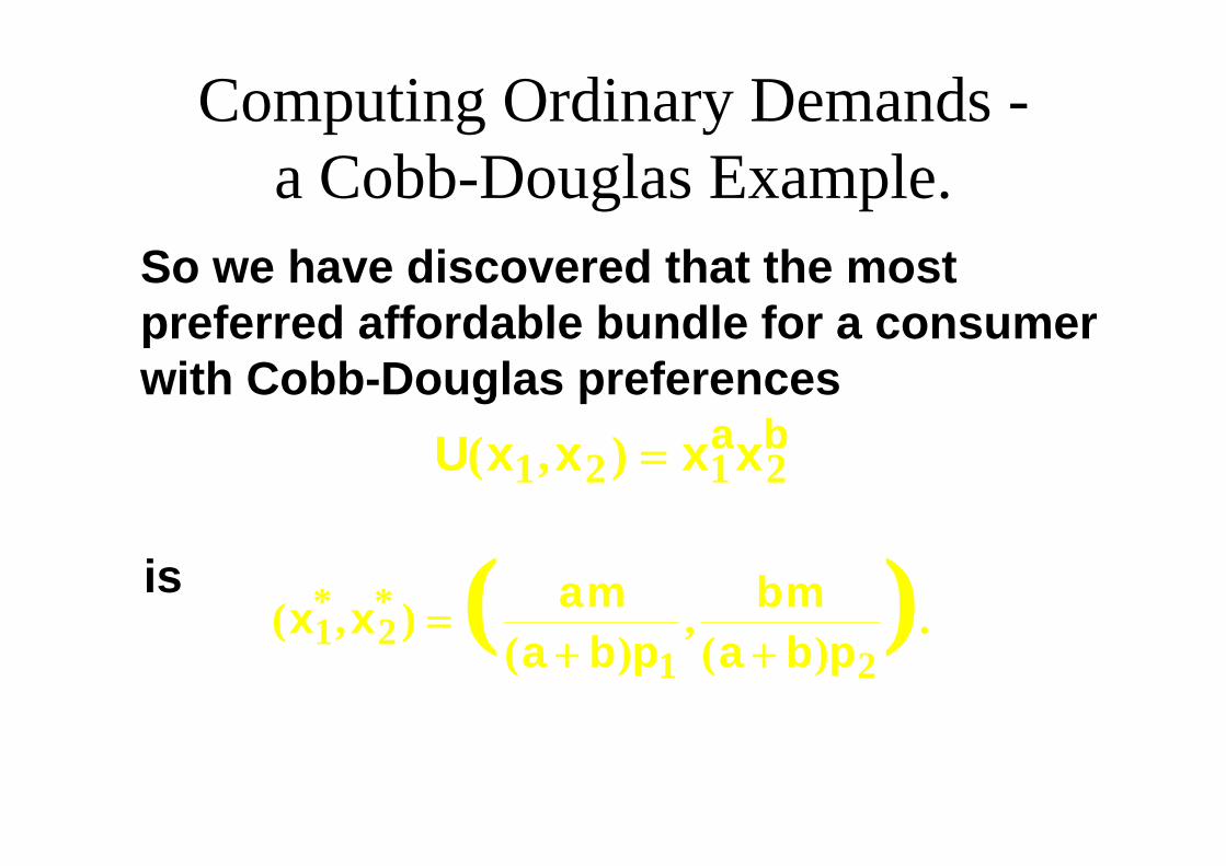
Computing Ordinary Demands -a Cobb-Douglas Example.
So we have discovered that the mostpreferred affordable bundle for a consumerpreferred affordable bundle for a consumerwith Cobb-Douglas preferences
a bU x x x xa b( , )1 2 1 2
is( , ) , .* * ( )x x am bm
1 2 ( , )( )
,( )
.( )x xa b p a b p1 2
1 2
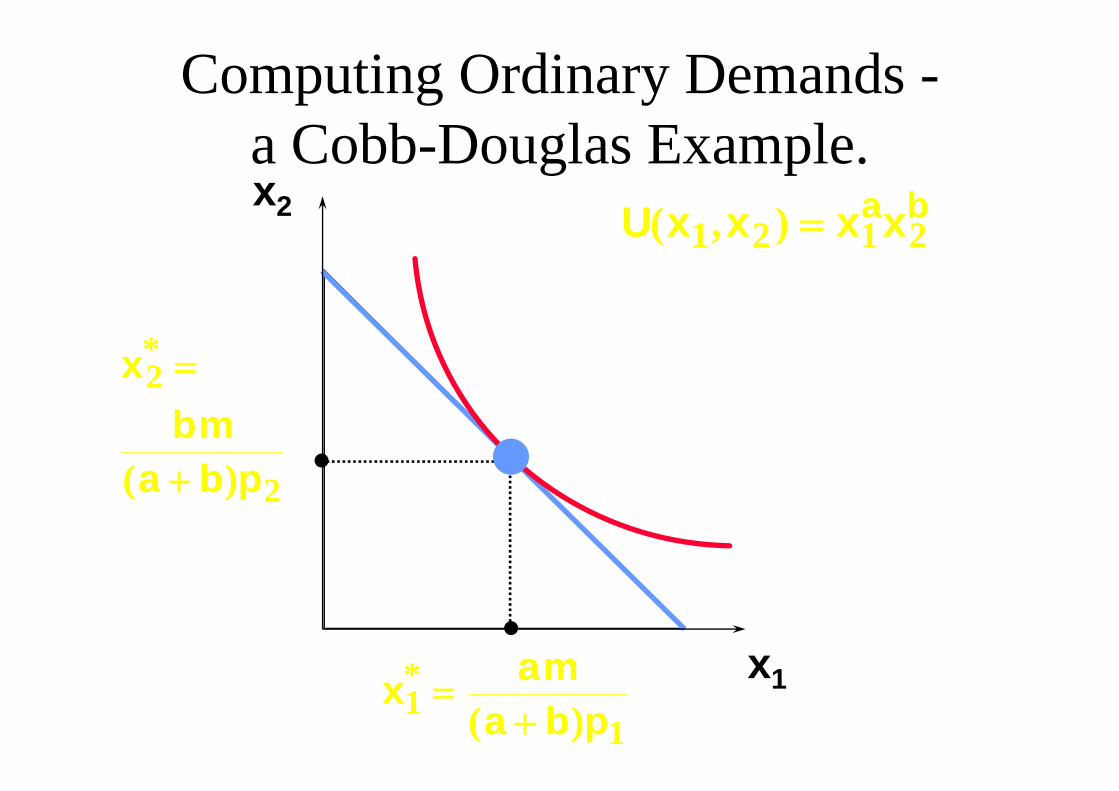
Computing Ordinary Demands -C bb D l E la Cobb-Douglas Example.
x2 U x x x xa b( )U x x x xa b( , )1 2 1 2
x2*
bma b p2( )a b p2( )
xam* x1x ama b p1
1
*( )

Rational Constrained ChoiceRational Constrained Choice When x1* > 0 and x2* > 0 1 2
and (x1*,x2*) exhausts the budget,and indifference curves have noand indifference curves have no
‘kinks’, the ordinary demands are obtained by solving:are obtained by solving:
(a) p1x1* + p2x2* = y (b) the slopes of the budget constraint,
-p /p and of the indifference curve-p1/p2, and of the indifference curve containing (x1*,x2*) are equal at (x1*,x2*).

Rational Constrained ChoiceRational Constrained Choice
But what if x1* = 0? Or if x * = 0? Or if x2* = 0? If either x1* = 0 or x2* = 0 then the
ordinary demand (x1*,x2*) is at a corner solution to the problem ofcorner solution to the problem of maximizing utility subject to a budget constraintconstraint.

Examples of Corner Solutions --the Perfect Substitutes Case
x2MRS = -1MRS 1
x11

Examples of Corner Solutions --the Perfect Substitutes Case
x2MRS = -1MRS 1
Slope = p /p with p > pSlope = -p1/p2 with p1 > p2.
x11

Examples of Corner Solutions --the Perfect Substitutes Case
x2MRS = -1MRS 1
Slope = p /p with p > pSlope = -p1/p2 with p1 > p2.
x11

Examples of Corner Solutions --the Perfect Substitutes Case
x2MRS = -1
x yp2
2
* MRS 1
Slope = p /p with p > pSlope = -p1/p2 with p1 > p2.
x1x1 0* 1x1 0

Examples of Corner Solutions --the Perfect Substitutes Case
x2MRS = -1MRS 1
Slope = p /p with p < p
*
Slope = -p1/p2 with p1 < p2.
x1x y*
x2 0
1x yp1
1

Examples of Corner Solutions --the Perfect Substitutes Case
So when U(x x ) = x + x the mostSo when U(x1,x2) = x1 + x2, the mostpreferred affordable bundle is (x1*,x2*)where
0,y)x,x( *2
*1 if p1 < p2
0,p
)x,x(1
21
and
if p1 < p2
and
** y0)xx( if p > p
2
21 py,0)x,x( if p1 > p2.

Examples of Corner Solutions --the Perfect Substitutes Case
x2MRS = -1MRS 1
Slope = -p1/p2 with p1 = p2.y
p2
x1y 1p1

Examples of Corner Solutions --the Perfect Substitutes Case
x2All the bundles in theAll the bundles in the constraint are equally the
most preferred affordable
yp2
most preferred affordablewhen p1 = p2.
x1y 1p1

Examples of Corner Solutions --the Non-Convex Preferences Casex2
x11

Examples of Corner Solutions --the Non-Convex Preferences Casex2
x11
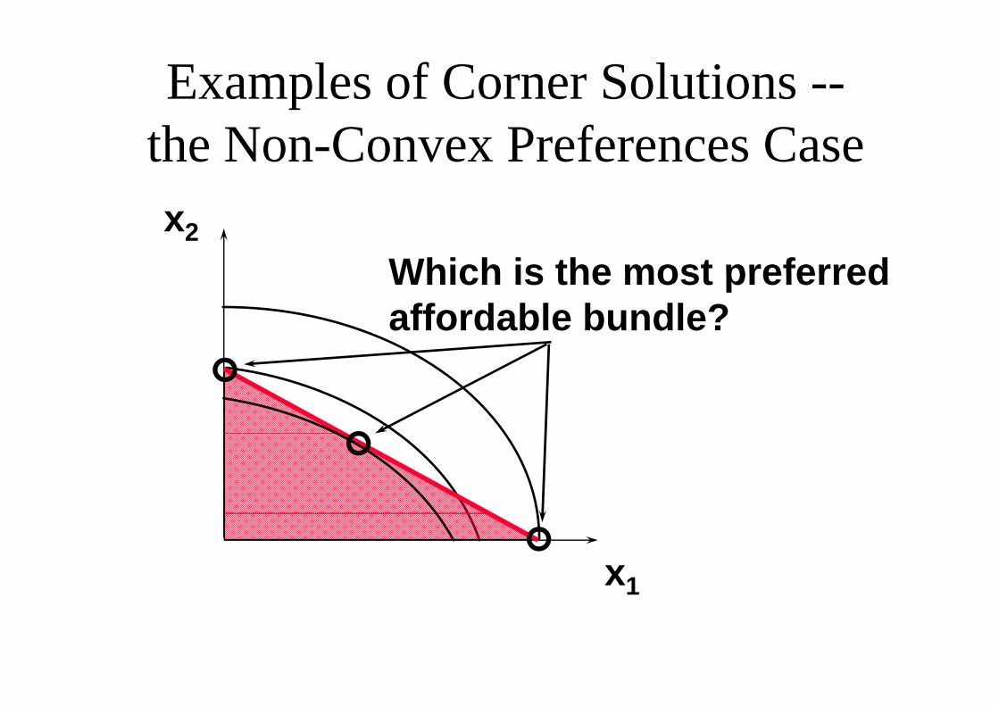
Examples of Corner Solutions --the Non-Convex Preferences Casex2
Which is the most preferredWhich is the most preferredaffordable bundle?
x11
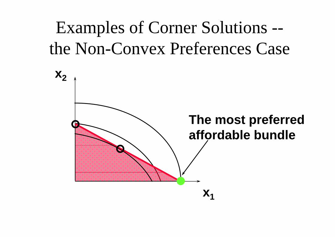
Examples of Corner Solutions --the Non-Convex Preferences Casex2
The most preferredThe most preferredaffordable bundle
x11
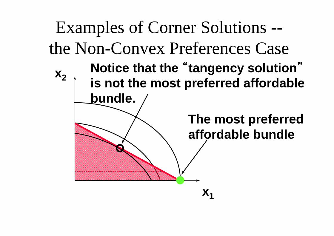
Examples of Corner Solutions --the Non-Convex Preferences Case
N ti th t th “t l ti ”x2Notice that the “tangency solution”is not the most preferred affordable
The most preferredbundle.
The most preferredaffordable bundle
x11

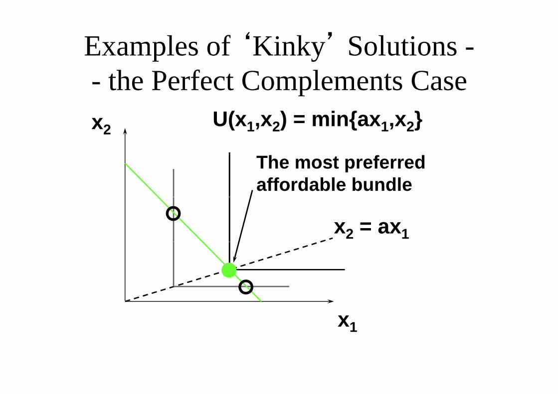
Examples of ‘Kinky’ Solutions -- the Perfect Complements Casex2 U(x1,x2) = min{ax1,x2}
x2 = ax1
x11

Examples of ‘Kinky’ Solutions -- the Perfect Complements Casex2 U(x1,x2) = min{ax1,x2}
x2 = ax1MRS = 0
x11

Examples of ‘Kinky’ Solutions -- the Perfect Complements Casex2 U(x1,x2) = min{ax1,x2}
MRS = -
x2 = ax1MRS = 0
x11

Examples of ‘Kinky’ Solutions -- the Perfect Complements Casex2 U(x1,x2) = min{ax1,x2}
MRS = - MRS is undefinedMRS is undefined
x2 = ax1MRS = 0
x11

Examples of ‘Kinky’ Solutions -- the Perfect Complements Casex2 U(x1,x2) = min{ax1,x2}
x2 = ax1
x11

Examples of ‘Kinky’ Solutions -- the Perfect Complements Casex2 U(x1,x2) = min{ax1,x2}
Which is the mostpreferred affordable bundle?
x2 = ax1
x11
Examples of ‘Kinky’ Solutions -- the Perfect Complements Casex2 U(x1,x2) = min{ax1,x2}
The most preferredaffordable bundle
x2 = ax1
x11

Examples of ‘Kinky’ Solutions -- the Perfect Complements Casex2 U(x1,x2) = min{ax1,x2}
x2 = ax1
x2*
x1x1* 1
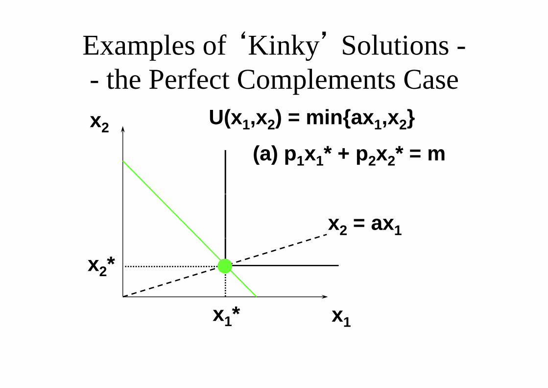
Examples of ‘Kinky’ Solutions -- the Perfect Complements Casex2 U(x1,x2) = min{ax1,x2}
(a) p x * + p x * = m(a) p1x1* + p2x2* = m
x2 = ax1
x2*
x1x1* 1

Examples of ‘Kinky’ Solutions -- the Perfect Complements Casex2 U(x1,x2) = min{ax1,x2}
(a) p x * + p x * = m(a) p1x1* + p2x2* = m(b) x2* = ax1*
x2 = ax1
x2*
x1x1* 1
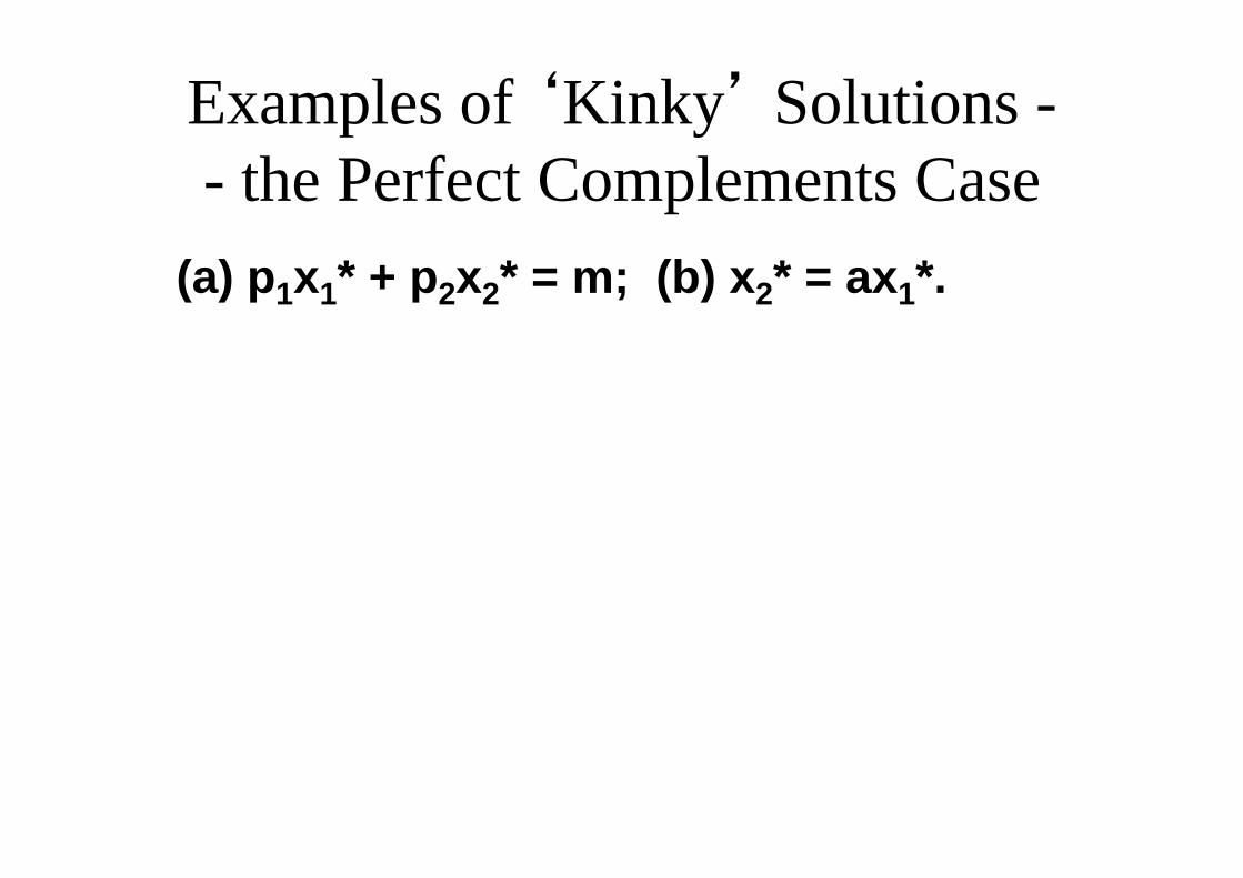
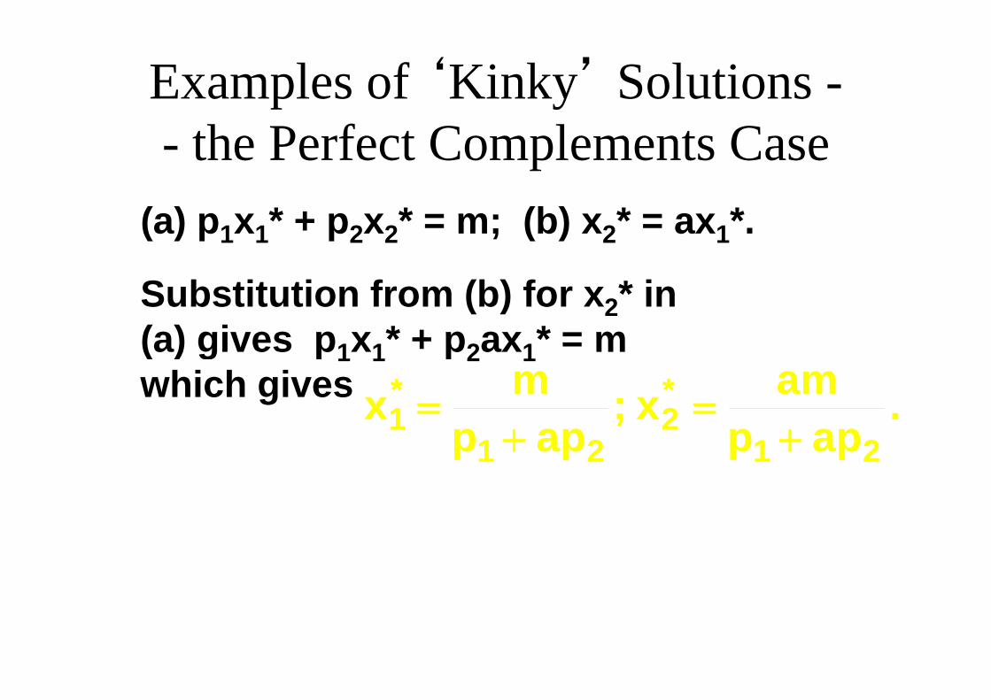
Examples of ‘Kinky’ Solutions -- the Perfect Complements Case
(a) p1x1* + p2x2* = m; (b) x2* = ax1*.
Examples of ‘Kinky’ Solutions -- the Perfect Complements Case
(a) p1x1* + p2x2* = m; (b) x2* = ax1*.
Substitution from (b) for x2* in (a) gives p1x1* + p2ax1* = m(a) gives p1x1 p2ax1 m

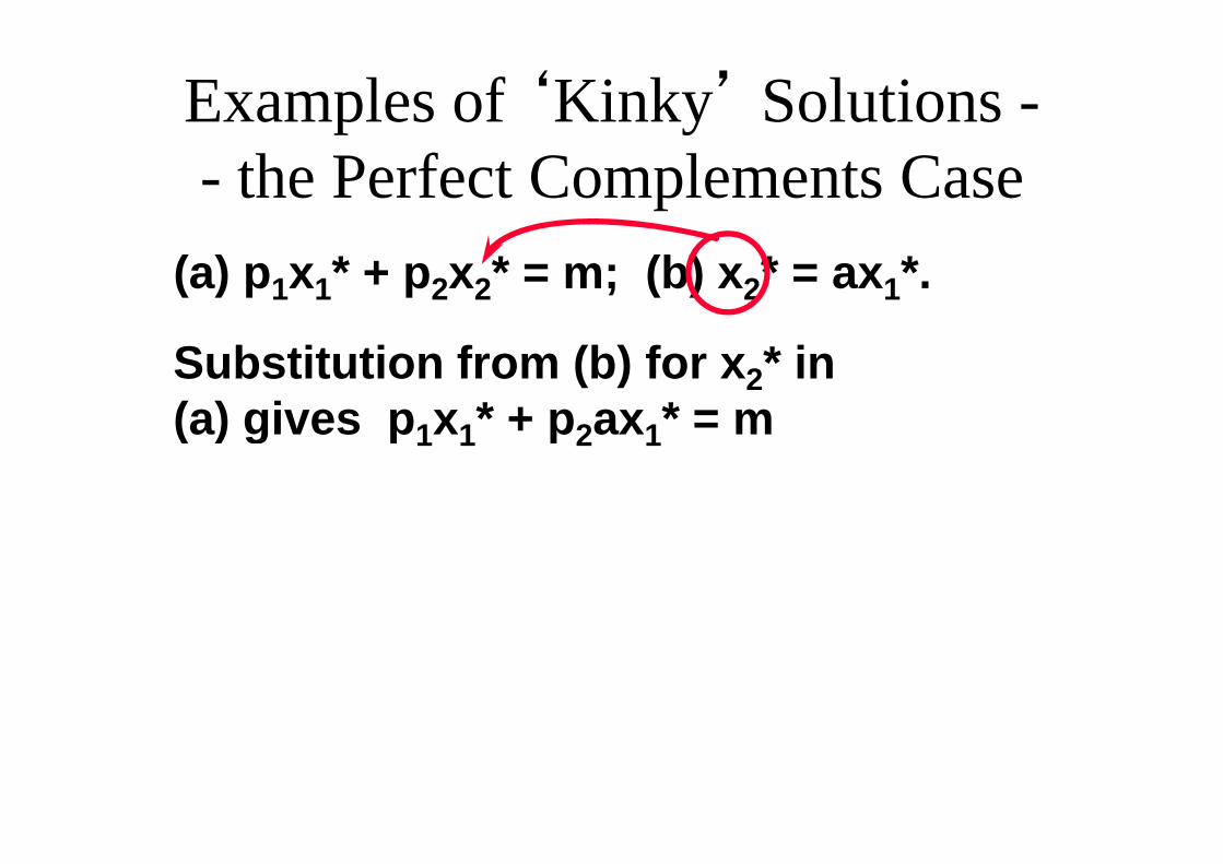
Examples of ‘Kinky’ Solutions -- the Perfect Complements Case
(a) p1x1* + p2x2* = m; (b) x2* = ax1*.
Substitution from (b) for x2* in (a) gives p1x1* + p2ax1* = m(a) gives p1x1 p2ax1 mwhich gives *
1 appmx
211 app
Examples of ‘Kinky’ Solutions -- the Perfect Complements Case
(a) p1x1* + p2x2* = m; (b) x2* = ax1*.
Substitution from (b) for x2* in (a) gives p1x1* + p2ax1* = m(a) gives p1x1 p2ax1 mwhich gives .
appamx;
appmx *
2*1
appapp 212
211

Examples of ‘Kinky’ Solutions -- the Perfect Complements Case
(a) p1x1* + p2x2* = m; (b) x2* = ax1*.
Substitution from (b) for x2* in (a) gives p1x1* + p2ax1* = m(a) gives p1x1 p2ax1 mwhich gives .
appamx;
appmx *
2*1
A bundle of 1 commodity 1 unit andappapp 21
221
1 y
a commodity 2 units costs p1 + ap2;m/(p1 + ap2) such bundles are affordable.m/(p1 + ap2) such bundles are affordable.

Examples of ‘Kinky’ Solutions -- the Perfect Complements Casex2 U(x1,x2) = min{ax1,x2}
x2 = ax1x2
*
amp ap1 2
x1x m1* 1p ap1
1 2


