
CHAPTER 8
CAPITAL STRUCTURE: THE OPTIMAL FINANCIAL MIX What is the optimal mix of debt and equity for a firm? In the last chapter we
looked at the qualitative trade-off between debt and equity, but we did not develop the
tools we need to analyze whether debt should be 0%, 20%, 40%, or 60% of capital. Debt
is always cheaper than equity, but using debt increases risk in terms of default risk to
lenders and higher earnings volatility for equity investors. Thus, using more debt can
increase value for some firms and decrease value for others, and for the same firm, debt
can be beneficial up to a point and destroy value beyond that point. We have to consider
ways of going beyond the generalities in the last chapter to specific ways of identifying
the right mix of debt and equity.
In this chapter, we explore four ways to find an optimal mix. The first approach
begins with a distribution of future operating income; we can then decide how much debt
to carry by defining the maximum possibility of default we are willing to bear. The
second approach is to choose the debt ratio that minimizes the cost of capital. We review
the role of cost of capital in valuation and discuss its relationship to the optimal debt
ratio. The third approach, like the second, also attempts to maximize firm value, but it
does so by adding the value of the unlevered firm to the present value of tax benefits and
then netting out the expected bankruptcy costs. The final approach is to base the
financing mix on the way comparable firms finance their operations.
Operating Income Approach The operating income approach is the simplest and one of the most intuitive ways
of determining how much a firm can afford to borrow. We determine a firm’s maximum
acceptable probability of default as our starting point, and based on the distribution of
operating income and cash flows, we then estimate how much debt the firm can carry.
Steps in Applying Operating Income Approach
We begin with an analysis of a firm’s operating income and cash flows, and we
consider how much debt it can afford to carry based on its cash flows. The steps in the
operating income approach are as follows:

1. We assess the firm’s capacity to generate operating income based on both current
conditions and past history. The result is a distribution for expected operating income,
with probabilities attached to different levels of income.
2. For any given level of debt, we estimate the interest and principal payments that have
to be made over time.
3. Given the probability distribution of operating income and the debt payments, we
estimate the probability that the firm will be unable to make those payments.
4. We set a limit or constraint on the probability of its being unable to meet debt
payments. Clearly, the more conservative the management of the firm, the tighter this
probability constraint will be.
5. We compare the estimated probability of default at a given level of debt to the
probability constraint. If the probability of default is higher than the constraint, the firm
chooses a lower level of debt; if it is lower than the constraint, the firm chooses a higher
level of debt.
Illustration 8.1: Estimating Debt Capacity Based on Operating Income Distribution
In the following analysis, we apply the operating income approach to analyzing
whether Disney should issue an additional $10 billion in new debt. We will assume that
Disney does not want the probability of being unable to make its total debt payments
from current operating income to exceed 5%.
Step 1: We derive a probability distribution for expected operating income from Disney’s
historical earnings and estimate percentage differences in operating income from 1988 to
2008 and present it in Figure 8.1.

The average change in operating income on an annual basis over the period was
13.26%, and the standard deviation in the annual changes is 19.80%. If we assume that
the changes are normally distributed, these statistics are sufficient for us to compute the
approximate probability of being unable to meet the specified debt payments.1
Step 2: We estimate the interest and principal payments on a proposed bond issue of $10
billion by assuming that the debt will be rated BBB, lower than Disney’s current bond
rating of A. Based on this rating, we estimated an interest rate of 7% on the debt. In
addition, we assume that the sinking fund payment set aside to repay the bonds is 10% of
the bond issue.2 This results in an annual debt payment of $1,700 million:
Additional Debt Payment = Interest Expense + Sinking Fund Payment
= 0.07 * $10,000 + 0.10 * $10,000 = $1,700 million
The total debt payment then can be computed by adding the interest payment of $728
million on existing debt and the operating lease expenses of $550 million (from the
1 Assuming income changes are normally distributed is undoubtedly a stretch. You can try alternative distributions that better fit the actual data. 2 A sinking fund payment allows a firm to set aside money to pay off a bond when it comes due at maturity in annual installments.

current year) to the additional debt payment that will be created by taking on $10 billion
in additional debt.
Total Debt Payment = Interest on Existing Debt + Operating Lease Expense + Additional
Debt Payment = $728 million + $550 million + $1,700 million = $ 2,978 million
Step 3: We can now estimate the probability of default3 from the distribution of operating
income. The simplest computation is to assume the percentage changes in operating
income are normally distributed, with the operating income of $6,726 million that Disney
earned the last four quarters, as the base year income, and the standard deviation of
19.8% from the historical data as the expected future standard deviation. The resulting t
statistic is 2.81:
t-Statistic = (Current EBIT – Debt Payment)/σOI (Current Operating Income)
= ($6,726 – $2.978)/(0.1980 * $6,726) = 2.81
Based on the t-statistic, the probability that Disney will be unable to meet its debt
payments in the next year is 0.24%.4
Step 4: Because the estimated probability of default is indeed less than 5%, Disney can
afford to borrow more than $10 billion. If the distribution of operating income changes is
normal, we can estimate the level of debt payments Disney can afford to make for a
probability of default of 5%.
t-Statistic for 5% probability level = 1.645
Consequently, the debt payment can be estimated as
($6,726 – X)/(0.1980 * $6,726) = 1.645
Solving for X, we estimate a breakeven debt payment of
Break-Even Debt Payment = $ 4,535 million
Subtracting out the existing interest and lease payments from this amount yields the
breakeven additional debt payment of $ 3,257 million.
Break-Even Additional Debt Payment = $4,535 – 728 – 550 = $ 3,257 million
3This is the probability of defaulting on interest payments in one period. The cumulative probability of default over time will be much higher. 4 This is likely to be a conservative estimate because it does not allow for the fact that Disney has a cash balance of $3,795 million that can be used to service debt, if the operating income falls short.

If we assume that the interest rate remains unchanged at 7% and the sinking fund will
remain at 10% of the outstanding debt, this yields an optimal additional debt of $ 19,161
million.
Optimal Additional Debt = Break-Even Additional Debt Payment/(Interest Rate +
Sinking Fund Rate)
= $3,257/(0.07 + 0.10) = $ 19,161 million
Based on this analysis, Disney should be able to more than double its existing debt
($16,682 million) and stay within its constraint of keeping the probability of default to
less than 5%.
Limitations of the Operating Income Approach
Although this approach may be intuitive and simple, it has key drawbacks. First,
estimating a distribution for operating income is not as easy as it sounds, especially for
firms in businesses that are changing and volatile. The operating income of firms can
vary widely from year to year, depending on the success or failure of individual products.
Second, even when we can estimate a distribution, the distribution may not fit the
parameters of a normal distribution, and the annual changes in operating income may not
reflect the risk of consecutive bad years. This can be remedied by calculating the
statistics based on multiple years of data. For Disney, if operating income is computed
over rolling two-year periods,5 the standard deviation will increase and the optimal debt
ratio will decrease.
This approach is also an extremely conservative way of setting debt policy
because it assumes that debt payments have to be made out of a firm’s operating income
and that the firm has no access to financial markets or pre-existing cash balance. Finally,
the probability constraint set by management is subjective and may reflect management
concerns more than stockholder interests. For instance, management may decide that it
wants no chance of default and refuse to borrow money as a consequence.
Refinements on the Operating Income Approach
The operating income approach described in this section is simplistic because it is
based on historical data and the assumption that operating income changes are normally 5By rolling two-year periods, we mean 1988-89, 1989-90 and so on for the rest of the data. 6 Opler, T., M. Saron and S. Titman, 1997, Designing Capital Structure to Create Stockholder Value, Journal of Applied Corporate Finance, v10, 21-32.
UnknownDeleted: ing of the same observations.

distributed. We can make it more sophisticated and robust by making relatively small
changes.
• We can look at simulations of different possible outcomes for operating income,
rather than looking at historical data; the distributions of the outcomes can be
based both on past data and on expectations for the future.
• Instead of evaluating just the risk of defaulting on debt, we can consider the
indirect bankruptcy costs that can accrue to a firm if operating income drops
below a specified level.
• We can compute the present value of the tax benefits from the interest payments
on the debt, across simulations, and thus compare the expected cost of bankruptcy
to the expected tax benefits from borrowing.
With these changes, we can look at different financing mixes for a firm and estimate the
optimal debt ratio as that mix that maximizes the firm’s value.6
Cost of Capital Approach In Chapter 4, we estimated the minimum acceptable hurdle rates for equity
investors (the cost of equity), and for all investors in the firm (the cost of capital). We
defined the cost of capital to be the weighted average of the costs of the different
components of financing—including debt, equity and hybrid securities—used by a firm
to fund its investments. By altering the weights of the different components, firms might
be able to change their cost of capital.7 In the cost of capital approach, we estimate the
costs of debt and equity at different debt ratios, use these costs to compute the costs of
capital, and look for the mix of debt and equity that yields the lowest cost of capital for
the firm. At this cost of capital, we will argue that firm value is maximized.
Cost of Capital and Maximizing Firm Value
In chapters 3 and 4, we laid the foundations for estimating the cost of capital for a
firm. We argued that the cost of equity should reflect the risk as perceived by the
marginal investors in the firm. If those marginal investors are diversified, the only risk
that should be priced in should be the risk that cannot be diversified away, captured in a
beta (in the CAPM) or betas (in multi factor models). If the marginal investors are not
diversified, the cost of equity may reflect some or all of the firm-specific risk in the firm. 7 If capital structure is irrelevant, the cost of capital will be unchanged as the capital structure is altered.

The cost of debt is a function of the default risk of the firm and reflects the current cost of
long term borrowing to the firm. Since interest is tax deductible, we adjust the cost of
debt for the tax savings, using the marginal tax rate, to estimate an after-tax cost. In
summary, the cost of capital is a weighted average of the costs of equity and debt, with
the weights based upon market values:
Cost of capital =
€
Cost of Equity Equity(Debt + Equity)
+ Cost of debt (1- t) Debt(Debt + Equity)
To understand the relationship between the cost of capital and optimal capital structure,
we first have to establish the relationship between firm value and the cost of capital. In
Chapter 5, we noted that the value of a project to a firm could be computed by
discounting the expected cash flows on it at a rate that reflected the riskiness of the cash
flows, and that the analysis could be done either from the viewpoint of equity investors
alone or from the viewpoint of the entire firm. In the latter approach, we discounted the
cash flows to the firm on the project, that is, the project cash flows prior to debt payments
but after taxes, at the project’s cost of capital.
Extending this principle, the value of the entire firm can be estimated by
discounting the aggregate expected cash flows to the firm over time at the firm’s cost of
capital. The firm’s aggregate cash flows can be estimated as cash flows after operating
expenses, taxes, and any capital investments needed to create future growth in both fixed
assets and working capital, but before debt payments.
Cash Flow to Firm = EBIT (1 – t) – (Capital Expenditures – Depreciation) –
Change in Non-cash Working Capital
The value of the firm can then be written as
€
Value of Firm = CF to Firmt
(1 +WACC)tt =1
t =∞
∑
The value of a firm is therefore a function of its cash flows and its cost of capital. In the
special case where the cash flows to the firm remain constant as the debt/equity mix is
changed, the value of the firm will increase as the cost of capital decreases. If the
objective in choosing the financing mix for the firm is the maximization of firm value,
this can be accomplished, in this case, by minimizing the cost of capital. In the more
general case where the cash flows to the firm themselves change as the debt ratio
changes, the optimal financing mix is the one that maximizes firm value.
The Cost of Capital Approach - Basics
To use the cost of capital approach in its simplest form, where the cash flows are
fixed and only the cost of capital changes, we need estimates of the cost of capital at
every debt ratio. In making these estimates, the one thing we cannot do is keep the costs
of debt and equity fixed, while changing the debt ratio. In addition to being unrealistic in
its assessment of risk as the debt ratio changes, this analysis will yield the unsurprising
conclusion that the cost of capital is minimized at a 100% debt ratio.
As the debt ratio increases, each of the components in the cost of capital will
change. Let us start with the equity component. Equity investors are entitled to the
residual earnings and cash flows in a firm, after interest and principal payments have
been made. As that firm borrows more money to fund a given level of assets, debt
payments will increase, and equity earnings will become more volatile. This higher
earnings volatility, in turn, will translate into a higher cost of equity. In the language of
the CAPM and multi-factor models, the beta or betas we use for equity should increase as
the debt ratio goes up. The debt holders will also see their risk increase as the firm
borrows more. Holding operating income constant, a firm that contracts to pay more to
debt holders has a greater chance of defaulting, which will result in a higher cost of debt.
As an added complication, the tax benefits of interest expenses can be put at risk, if these
expenses become greater than the earnings.
The key to using the cost of capital approach is coming up with realistic estimates
of the cost of equity and debt at different debt ratios. The optimal financing mix for a
firm is trivial to compute if one is provided with a schedule that relates the costs of equity
and debt to the debt ratio of the firm. Computing the optimal debt ratio then becomes
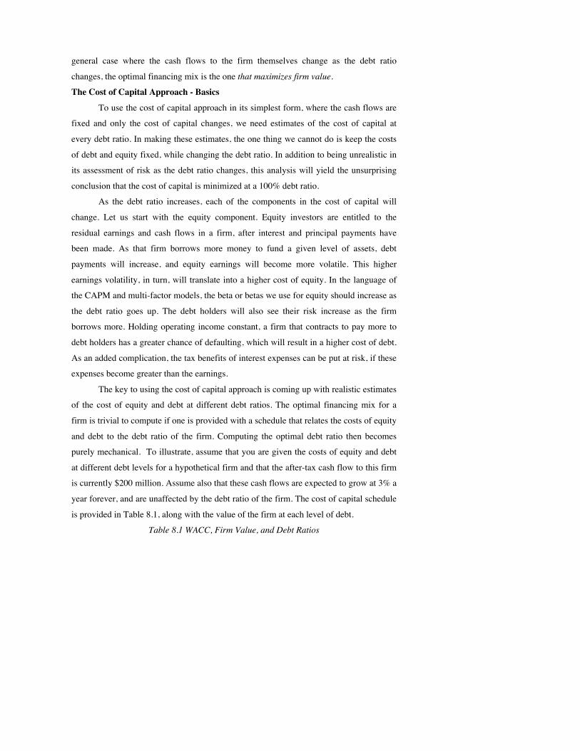
purely mechanical. To illustrate, assume that you are given the costs of equity and debt
at different debt levels for a hypothetical firm and that the after-tax cash flow to this firm
is currently $200 million. Assume also that these cash flows are expected to grow at 3% a
year forever, and are unaffected by the debt ratio of the firm. The cost of capital schedule
is provided in Table 8.1, along with the value of the firm at each level of debt.
Table 8.1 WACC, Firm Value, and Debt Ratios
D/(D+E) Cost of Equity After-tax Cost of Debt Cost of Capital Firm Value 0 10.50% 4.80% 10.50% $2,747
10% 11.00% 5.10% 10.41% $2,780 20% 11.60% 5.40% 10.36% $2,799 30% 12.30% 5.52% 10.27% $2,835 40% 13.10% 5.70% 10.14% $2,885 50% 14.00% 6.10% 10.15% $2,922 60% 15.00% 7.20% 10.32% $2,814 70% 16.10% 8.10% 10.50% $2,747 80% 17.20% 9.00% 10.64% $2,696 90% 18.40% 10.20% 11.02% $2,569 100% 19.70% 11.40% 11.40% $2,452
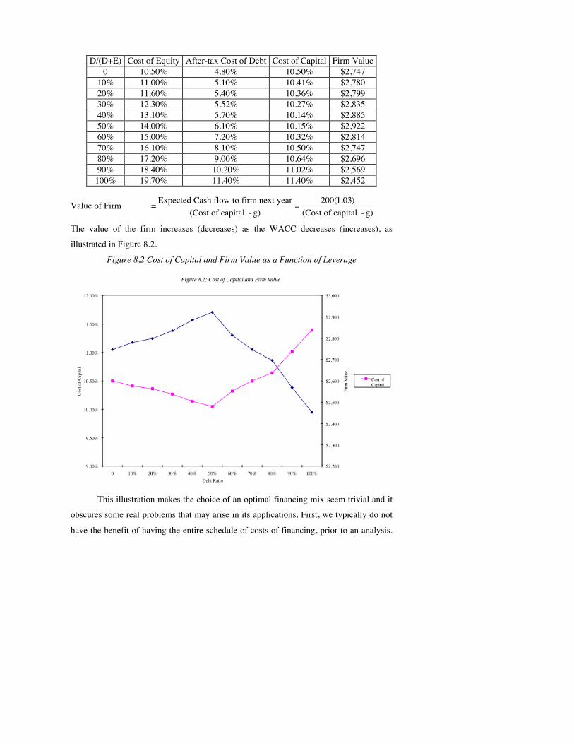
Value of Firm =
€
Expected Cash flow to firm next year(Cost of capital - g)
=200(1.03)
(Cost of capital - g)
The value of the firm increases (decreases) as the WACC decreases (increases), as
illustrated in Figure 8.2.
Figure 8.2 Cost of Capital and Firm Value as a Function of Leverage
This illustration makes the choice of an optimal financing mix seem trivial and it
obscures some real problems that may arise in its applications. First, we typically do not
have the benefit of having the entire schedule of costs of financing, prior to an analysis.

In most cases, the only level of debt about which there is any certainty about the cost of
financing is the current level. Second, the analysis assumes implicitly that the level of
cash flows to the firm is unaffected by the financing mix of the firm and consequently by
the default risk (or bond rating) for the firm. Although this may be reasonable in some
cases, it might not in others. For instance, a firm that manufactures consumer durables
(cars, televisions, etc.) might find that its sales and operating income drop if its default
risk increases because investors are reluctant to buy its products. We will deal with the
computational component of estimating costs of debt, equity and capital first in the
standard cost of capital approach and then follow up by examining how to bring in
changes in expected cash flows into the analysis in the enhanced cost of capital approach.
8.1. Minimizing Cost of Capital and Maximizing Firm Value
A lower cost of capital will lead to a higher firm value only if
a. the operating income does not change as the cost of capital declines.
b. the operating income goes up as the cost of capital goes down.
c. any decline in operating income is offset by the lower cost of capital.
The Standard Cost of Capital Approach
In the standard cost of capital approach, we keep the operating income and cash
flows fixed, while changing the cost of capital. Not surprisingly, the optimal debt ratio is
the one that minimizes the cost of capital. While the assumptions seem heroic, it is a good
starting point for the discussion.
Steps in computing cost of capital
We need three basic inputs to compute the cost of capital—the cost of equity, the
after-tax cost of debt, and the weights on debt and equity. The costs of equity and debt
change as the debt ratio changes, and the primary challenge of this approach is in
estimating each of these inputs.
Let us begin with the cost of equity. In Chapter 4, we argued that the beta of equity
will change as the debt ratio changes. In fact, we estimated the levered beta as a function
of the debt to equity ratio of a firm, the unlevered beta, and the firm’s marginal tax rate:
βlevered = βunlevered [1 + (1 – t)Debt/Equity]

Thus, if we can estimate the unlevered beta for a firm, we can use it to computed the
levered beta of the firm at every debt ratio. This levered beta can then be used to compute
the cost of equity at each debt ratio.
Cost of Equity = Risk-Free Rate + βlevered (Risk Premium)
The cost of debt for a firm is a function of the firm’s default risk. As firms borrow
more, their default risk will increase and so will the cost of debt. If we use bond ratings as
the measure of default risk, we can estimate the cost of debt in three steps. First, we
estimate a firm’s dollar debt and interest expenses at each debt ratio; as firms increase
their debt ratio, both dollar debt and interest expenses will rise. Second, at each debt
level, we compute a financial ratio or ratios that measure default risk and use the ratio(s)
to estimate a rating for the firm; again, as firms borrow more, this rating will decline.
Third, a default spread, based on the estimated rating, is added on to the risk-free rate to
arrive at the pretax cost of debt. Applying the marginal tax rate to this pretax cost yields
an after-tax cost of debt.
Once we estimate the costs of equity and debt at each debt level, we weight them
based on the proportions used of each to estimate the cost of capital. Although we have
not explicitly allowed for a preferred stock component in this process, we can have
preferred stock as a part of capital. However, we have to keep the preferred stock portion
fixed while changing the weights on debt and equity. The debt ratio at which the cost of
capital is minimized is the optimal debt ratio.
In this approach, the effect of changing the capital structure, on firm value, is
isolated by keeping the operating income fixed, and varying only the cost of capital. In
practical terms, this requires us to make two assumptions. First, the debt ratio is
decreased by raising new equity and retiring debt; conversely, the debt ratio is increased
by borrowing money and buying back stock. This process is called recapitalization.
Second, the pretax operating income is assumed to be unaffected by the firm’s financing
mix and, by extension, its bond rating. If the operating income changes with a firm’s
default risk, the basic analysis will not change, but minimizing the cost of capital may not
be the optimal course of action, because the value of the firm is determined by both the
cash flows and the cost of capital. The value of the firm will have to be computed at each
debt level and the optimal debt ratio will be that which maximizes firm value.

Illustration 8.2: Analyzing the Capital Structure for Disney: May 2009
The cost of capital approach can be used to find the optimal capital structure for a
firm, as we will for Disney in May 2009. Disney had $16,003 million in interest-bearing
debt on its books and we estimated the market value of this debt to be $14,962 million in
chapter 4. Adding the present value of operating leases of $1,720 million (also estimated
in chapter 4) to this value, we arrive at a total market value for the debt of $16,682
million. The market value of equity at the same time was $45,193 million; the market
price per share was $24.34, and there were 1856.752 million shares outstanding.
Proportionally, 26.96% of the overall financing mix was debt, and the remaining 73.04%
was equity.
The beta for Disney’s stock in May 2009, as estimated in Chapter 4, was 0.9011.
The Treasury bond rate at that time was 3.5%. Using an estimated equity risk premium of
6%, we estimated the cost of equity for Disney to be 8.91%:
Cost of Equity = Risk-Free Rate + Beta * (Market Premium)
= 3.5% + 0.9011(6%) = 8.91%
Disney’s bond rating in May 2009 was A, and based on this rating, the estimated pretax
cost of debt for Disney is 6%. Using a marginal tax rate of 38%, we estimate the after-tax
cost of debt for Disney to be 3.72%.
After-Tax Cost of Debt = Pretax Interest Rate (1 – Tax Rate)
= 6.00% (1 – 0.38) = 3.72%
The cost of capital was calculated using these costs and the weights based on market value:
Cost of capital =
€
Cost of Equity Equity(Debt + Equity)
+ Cost of debt (1- t) Debt(Debt + Equity)
=
€
8.91% 45,193(16,682 + 45,193)
+ 3.72% 16,682(16,682 + 45,193)
= 7.51%
8.2. Market Value, Book Value, and Cost of Capital
Disney had a book value of equity of approximately $32.7 billion and a book value of
debt of $16 billion. If you held the cost of equity and debt constant and replaced the
market value weights in the cost of capital with book value weights, you will end up with
a. A lower cost of capital
b. A higher cost of capital
c. The same cost of capital
What are the implications for valuation?
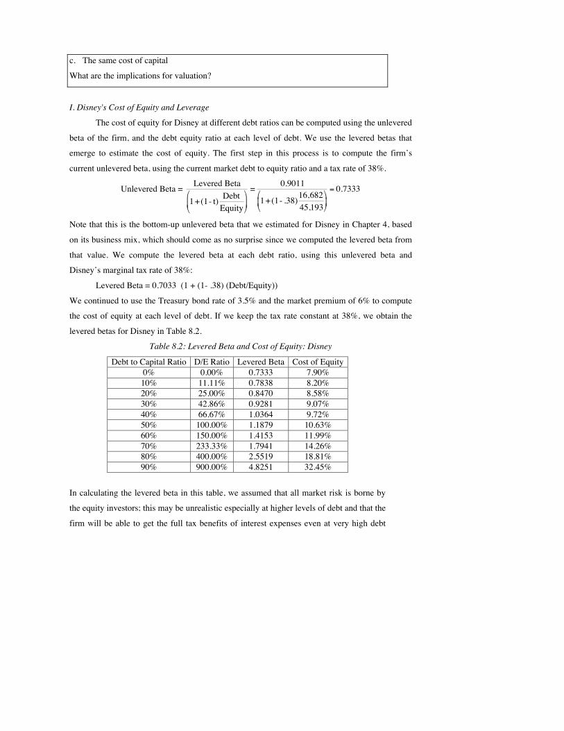
I. Disney's Cost of Equity and Leverage
The cost of equity for Disney at different debt ratios can be computed using the unlevered
beta of the firm, and the debt equity ratio at each level of debt. We use the levered betas that
emerge to estimate the cost of equity. The first step in this process is to compute the firm’s
current unlevered beta, using the current market debt to equity ratio and a tax rate of 38%.
Unlevered Beta =
€
Levered Beta
1+(1- t) DebtEquity
= 0.9011
1+(1- .38)16,68245,193
= 0.7333
Note that this is the bottom-up unlevered beta that we estimated for Disney in Chapter 4, based
on its business mix, which should come as no surprise since we computed the levered beta from
that value. We compute the levered beta at each debt ratio, using this unlevered beta and
Disney’s marginal tax rate of 38%:
Levered Beta = 0.7033 (1 + (1- .38) (Debt/Equity))
We continued to use the Treasury bond rate of 3.5% and the market premium of 6% to compute
the cost of equity at each level of debt. If we keep the tax rate constant at 38%, we obtain the
levered betas for Disney in Table 8.2.
Table 8.2: Levered Beta and Cost of Equity: Disney
Debt to Capital Ratio D/E Ratio Levered Beta Cost of Equity 0% 0.00% 0.7333 7.90%
10% 11.11% 0.7838 8.20% 20% 25.00% 0.8470 8.58% 30% 42.86% 0.9281 9.07% 40% 66.67% 1.0364 9.72% 50% 100.00% 1.1879 10.63% 60% 150.00% 1.4153 11.99% 70% 233.33% 1.7941 14.26% 80% 400.00% 2.5519 18.81% 90% 900.00% 4.8251 32.45%
In calculating the levered beta in this table, we assumed that all market risk is borne by
the equity investors; this may be unrealistic especially at higher levels of debt and that the
firm will be able to get the full tax benefits of interest expenses even at very high debt

ratios. We will also consider an alternative estimate of levered betas that apportions some
of the market risk to the debt:
βlevered = βu[1 + (1 – t)D/E] – βdebt (1 – t)D/E
The beta of debt can be based on the rating of the bond, estimated by regressing past
returns on bonds in each rating class against returns on a market index or backed out of
the default spread. The levered betas estimated using this approach will generally be
lower than those estimated with the conventional model.8 We will also examine whether
the full benefits of interest expenses will accrue at higher debt ratios.
II. Disney’s Cost of Debt and Leverage
There are several financial ratios that are correlated with bond ratings, and we
face two choices. One is to build a model that includes several financial ratios to estimate
the synthetic ratings at each debt ratio. In addition to being more labor and data intensive,
the approach will make the ratings process less transparent and more difficult to decipher.
The other is to stick with the simplistic approach that we developed in chapter 4, of
linking the rating to the interest coverage ratio, with the ratio defined as:
Interest Coverage Ratio =
€
Earnings before interest and taxesInterest Expenses
We will stick with the simpler approach for three reasons. First, we are not aiming for
precision in the cost of debt, but an approximation. Given that the more complex
approaches also give you approximations, we will tilt in favor of transparency. Second,
there is significant correlation not only between the interest coverage ratio and bond
ratings but also between the interest coverage ratio and other ratios used in analysis, such
as the debt coverage ratio and the funds flow ratios. In other words, we may be adding
little by adding other ratios that are correlated with interest coverage ratios, including
EBITDA/Fixed Charges, to the mix. Third, the interest coverage ratio changes as a firm
changes is financing mix and decreases as the debt ratio increases, a key requirement
since we need the cost of debt to change as the debt ratio changes.
8 Consider, for instance, a debt ratio of 40 percent. At this level the firm’s debt will take on some of the characteristics of equity. Assume that the beta of debt at a 40 percent debt ratio is 0.10. The equity beta at that debt ratio can be computed as follows:
Levered Beta = 0.7333 (1 + (1 – 0.38)(40/60) – 0.10 (1 – 0.373) (40/60) = 0.99 In the unadjusted approach, the levered beta would have been 1.0364.
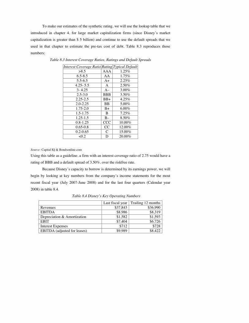
To make our estimates of the synthetic rating, we will use the lookup table that we
introduced in chapter 4, for large market capitalization firms (since Disney’s market
capitalization is greater than $ 5 billion) and continue to use the default spreads that we
used in that chapter to estimate the pre-tax cost of debt. Table 8.3 reproduces those
numbers:
Table 8.3 Interest Coverage Ratios, Ratings and Default Spreads
Interest Coverage Ratio Rating Typical Default >8.5 AAA 1.25%
6.5-8.5 AA 1.75% 5.5-6.5 A+ 2.25%
4.25- 5.5 A 2.50% 3- 4.25 A– 3.00% 2.5-3.0 BBB 3.50%
2.25-2.5 BB+ 4.25% 2.0-2.25 BB 5.00% 1.75-2.0 B+ 6.00% 1.5-1.75 B 7.25% 1.25-1.5 B– 8.50% 0.8-1.25 CCC 10.00% 0.65-0.8 CC 12.00% 0.2-0.65 C 15.00%
<0.2 D 20.00%
Source: Capital IQ & Bondsonline.com
Using this table as a guideline, a firm with an interest coverage ratio of 2.75 would have a
rating of BBB and a default spread of 3.50%, over the riskfree rate.
Because Disney’s capacity to borrow is determined by its earnings power, we will
begin by looking at key numbers from the company’s income statements for the most
recent fiscal year (July 2007-June 2008) and for the last four quarters (Calendar year
2008) in table 8.4.
Table 8.4 Disney’s Key Operating Numbers
Last fiscal year Trailing 12 months Revenues $37,843 $36,990 EBITDA $8,986 $8,319 Depreciation & Amortization $1,582 $1,593 EBIT $7,404 $6,726 Interest Expenses $712 $728 EBITDA (adjusted for leases) $9,989 $8,422

EBIT( adjusted for leases) $7,708 $6,829 Interest Expenses (adjusted for leases) $815 $831
Note that converting leases to debt affects both the operating income and the interest
expense; the imputed interest expense on the lease debt is added to both the operating
income and interest expense numbers.9 Since the trailing 12-month figures represent
more recent information, we will use those numbers in assessing Disney’s optimal debt
ratio. Based on the EBIT (adjusted for leases) of $6,829 million and interest expenses of
$831 million, Disney has an interest coverage ratio of 8.22 and should command a rating
of AA, two notches above its actual rating of A.
To compute Disney’s ratings at different debt levels, we start by assessing the
dollar debt that Disney will need to issue to get to the specified debt ratio. This can be
accomplished by multiplying the total market value of the firm today by the desired debt
to capital ratio. To illustrate, Disney’s dollar debt at a 10% debt ratio will be $6,188
million, computed thus:
Value of Disney = Current Market Value of Equity + Current Market Value of Debt
= 45,193 + $16,682 = $61,875 million
$ Debt at 10% Debt to Capital Ratio = 10% of $61,875 = $6,188 million
The second step in the process is to compute the interest expense that Disney will have at
this debt level, by multiplying the dollar debt by the pre-tax cost of borrowing at that debt
ratio. The interest expense is then used to compute an interest coverage ratio which is
employed to compute a synthetic rating. The resulting default spread, based on the rating,
can be obtained from table 8.3, and adding the default spread to the riskfree rate yields a
pre-tax cost of borrowing. Table 8.5 estimates the interest expenses, interest coverage
ratios, and bond ratings for Disney at 0% and 10% debt ratios, at the existing level of
operating income.
Table 8.5 Effect of Moving to Higher Debt Ratios: Disney
D/(D + E) 0.00% 10.00%
9 The present value of operating leases ($1,720 million) was multiplied by the pre-tax cost of debt of 6% to arrive at an interest expense of $ 103 million, which is added to both operating income and interest expense. Multiplying the pretax cost of debt by the present value of operating leases yields an approximation. The full adjustment would require us to add back the entire operating lease expense and to subtract out the depreciation on the leased asset.

D/E 0.00% 11.11% $ Debt $0 $6,188 EBITDA $8,422 $8,422 Depreciation $1,593 $1,593 EBIT $6,829 $6,829 Interest $0 $294 Pretax int. cov ∞ 23.24 Likely rating AAA AAA Pretax cost of debt 4.75% 4.75%
Note that the EBITDA and EBIT remain fixed as the debt ratio changes. We ensure this
by using the proceeds from the debt to buy back stock, thus leaving operating assets
untouched and isolating the effect of changing the debt ratio.
There is circular reasoning involved in estimating the interest expense. The
interest rate is needed to calculate the interest coverage ratio, and the coverage ratio is
necessary to compute the interest rate. To get around the problem, we began our analysis
by assuming that Disney could borrow $6,188 billion at the AAA rate of 4.75%; we then
compute an interest expense and interest coverage ratio using that rate. At the 10% debt
ratio, our life was simplified by the fact that the rating remained unchanged at AAA. To
illustrate a more difficult step up in debt, consider the change in the debt ratio from 20%
to 30%:
Iteration 1
(Debt @AAA rate) Iteration 2
(Debt @AA rate) D/(D + E) 20.00% 30.00% 30.00% D/E 25.00% 42.86% 42.86% $ Debt $12,375 $ 18,563 $18,563 EBITDA $8,422 $8,422 $8,422 Depreciation $1,593 $1,593 $1,593 EBIT $6,829 $6,829 $6,829 Interest $588 18563*.0475=$881 18563*.0525 =$974 Pretax int. cov 11.62 7.74 7.01 Likely rating AAA AA AA Pretax cost of debt 4.75% 5.25% 5.25%
While the initial estimate of the interest expenses at the 30% debt ratio reflects the AAA
rating and 4.75% interest rate) that the firm enjoyed at the 20% debt ratio, the resulting
interest coverage ratio of 7.74 pushes the rating down to AA and the interest rate to
5.25%. Consequently, we have to recompute the interest expenses at the higher rate (in
iteration 2) and reach steady state: the interest rate that we use matches up to the

estimated interest rate.10 This process is repeated for each level of debt from 10% to 90%,
and the iterated after-tax costs of debt are obtained at each level of debt in Table 8.6.
Table 8.6 Disney: Cost of Debt and Debt Ratios
Debt Ratio $ Debt
Interest Expense
Interest coverage
ratio Bond Rating
Interest rate on debt
Tax Rate
After-tax cost of debt
0% $0 $0 ∞ AAA 4.75% 38.00% 2.95% 10% $6,188 $294 23.24 AAA 4.75% 38.00% 2.95% 20% $12,375 $588 11.62 AAA 4.75% 38.00% 2.95% 30% $18,563 $975 7.01 AA 5.25% 38.00% 3.26% 40% $24,750 $1,485 4.60 A 6.00% 38.00% 3.72% 50% $30,938 $2,011 3.40 A- 6.50% 38.00% 4.03% 60% $37,125 $2,599 2.63 BBB 7.00% 38.00% 4.34% 70% $43,313 $5,198 1.31 B- 12.00% 38.00% 7.44% 80% $49,500 $6,683 1.02 CCC 13.50% 38.00% 8.37% 90% $55,688 $7,518 0.91 CCC 13.50% 34.52% 8.84%
Note that the interest expenses increase more than proportionately as the debt
increases, since the cost of debt rises with the debt ratio. There are three points to make
about these computations.
a. At each debt ratio, we compute the dollar value of debt by multiplying the debt
ratio by the existing market value of the firm ($61,875 million). In reality, the
value of the firm will change as the cost of capital changes and the dollar debt that
we will need to get to a specified debt ratio, say 30%, will be different from the
values that we have estimated. The reason that we have not tried to incorporate
this effect is that it leads more circularity in our computations, since the value at
each debt ratio is a function of the savings from the interest expenses at that debt
ratio, which in turn, will depend upon the value.
b. We assume that at every debt level, all existing debt will be refinanced at the new
interest rate that will prevail after the capital structure change. For instance,
Disney’s existing debt, which has a A rating, is assumed to be refinanced at the
interest rate corresponding to a A- rating when Disney moves to a 50% debt ratio.
This is done for two reasons. The first is that existing debt holders might have
10 Because the interest expense rises, it is possible for the rating to drop again. Thus, a third iteration might be necessary in some cases.

protective puts that enable them to put their bonds back to the firm and receive
face value.11 The second is that the refinancing eliminates “wealth expropriation”
effects—the effects of stockholders expropriating wealth from bondholders when
debt is increased, and vice versa when debt is reduced. If firms can retain old debt
at lower rates while borrowing more and becoming riskier, the lenders of the old
debt will lose value. If we lock in current rates on existing bonds and recalculate
the optimal debt ratio, we will allow for this wealth transfer. 12
c. Although it is conventional to leave the marginal tax rate unchanged as the debt
ratio is increased, we adjust the tax rate to reflect the potential loss of the tax
benefits of debt at higher debt ratios, where the interest expenses exceed the
EBIT. To illustrate this point, note that the EBIT at Disney is $6,829 million. As
long as interest expenses are less than $6,829 million, interest expenses remain
fully tax-deductible and earn the 38% tax benefit. For instance, even at an 80%
debt ratio, the interest expenses are $6,683million and the tax benefit is therefore
38% of this amount. At a 90% debt ratio, however, the interest expenses balloon
to $7,518 million, which is greater than the EBIT of $6,829 million. We consider
the tax benefit on the interest expenses up to this amount:
Maximum Tax Benefit = EBIT * Marginal Tax Rate = $6,829 million *
0.38 = $2,595 million
As a proportion of the total interest expenses, the tax benefit is now only 34.52%:
Adjusted Marginal Tax Rate = Maximum Tax Benefit/Interest Expenses =
$2,595/$7,518 = 34.52%
This in turn raises the after-tax cost of debt. This is a conservative approach,
because losses can be carried forward. Given that this is a permanent shift in
leverage, it does make sense to be conservative. We used this tax rate to
recompute the levered beta at a 90% debt ratio, to reflect the fact that tax savings
from interest are depleted.
11 If they do not have protective puts, it is in the best interests of the stockholders not to refinance the debt if debt ratios are increased. 12 This will have the effect of reducing interest cost, when debt is increased, and thus interest coverage ratios. This will lead to higher ratings, at least in the short term, and a higher optimal debt ratio.

III. Leverage and Cost of Capital
Now that we have estimated the cost of equity and the cost of debt at each debt
level, we can compute Disney’s cost of capital. This is done for each debt level in Table
8.7. The cost of capital, which is 7.90% when the firm is unlevered, decreases as the firm
initially adds debt, reaches a minimum of 7.32% at a 40% debt ratio, and then starts to
increase again. (See table 8.10 for the full details of the numbers in this table)
Table 8.7 Cost of Equity, Debt, and Capital, Disney
Debt Ratio Beta Cost of Equity Cost of Debt (after-tax) Cost of capital 0% 0.73 7.90% 2.95% 7.90% 10% 0.78 8.20% 2.95% 7.68% 20% 0.85 8.58% 2.95% 7.45% 30% 0.93 9.07% 3.26% 7.32% 40% 1.04 9.72% 3.72% 7.32% 50% 1.19 10.63% 4.03% 7.33% 60% 1.42 11.99% 4.34% 7.40% 70% 1.79 14.26% 7.44% 9.49% 80% 2.55 18.81% 8.37% 10.46% 90% 5.05 33.83% 8.84% 11.34%
Note that we are moving in 10% increments and that the cost of capital flattens out
between 30 and 50%. We can get a more precise reading of the optimal by looking at
how the cost of capital moves between 30 and 50%, in smaller increments. Using 1%
increments, the optimal debt ratio that we compute for Disney is 43%. with a cost of
capital of 7.28%. The optimal cost of capital is shown graphically in figure 8.3. We will
stick with the approximate optimal of 40% the rest of this chapter.

To illustrate the robustness of this solution to alternative measures of levered
betas, we reestimate the costs of debt, equity, and capital under the assumption that debt
bears some market risk; the results are summarized in Table 8.8.
Table 8.8 Costs of Equity, Debt, and Capital with Debt Carrying Market Risk, Disney
Debt Ratio Beta of Equity Beta of Debt Cost of Equity Cost of Debt (after-tax) Cost of capital 0% 0.73 0.05 7.90% 2.95% 7.90%
10% 0.78 0.05 8.18% 2.95% 7.66% 20% 0.84 0.05 8.53% 2.95% 7.42% 30% 0.91 0.07 8.95% 3.26% 7.24% 40% 0.99 0.10 9.46% 3.72% 7.16% 50% 1.11 0.13 10.16% 4.03% 7.10% 60% 1.28 0.00 11.18% 4.34% 7.08% 70% 1.28 0.35 11.19% 7.44% 8.57% 80% 1.52 0.42 12.61% 8.37% 9.22% 90% 2.60 0.42 19.10% 8.84% 9.87%

If the debt holders bear some market risk, the cost of equity is lower at higher levels of
debt, and Disney’s optimal debt ratio increases to 60%, higher than the optimal debt ratio
of 40% that we computed using the conventional beta measure.13
IV. Firm Value and Cost of Capital
The reason for minimizing the cost of capital is that it maximizes the value of the
firm. To illustrate the effects of moving to the optimal on Disney’s firm value, we start
off with a simple valuation model, designed to value a firm in stable growth.
Firm Value =
€
Expected Cash flow to firmNext year
(Cost of capital - g)
where g is the growth rate in the cash flow to the firm (in perpetuity. We begin by
computing Disney’s current free cash flow using its current earnings before interest and
taxes of $6,829 million, its tax rate of 38%, and its reinvestment in 2008 in long term
assets (ignoring working capital):14
EBIT (1 – Tax Rate) = 6829 (1 – 0.38) = $4,234
+ Depreciation and amortization = $1,593
– Capital expenditures = $1,628
– Change in noncash working capital $0
Free cash flow to the firm = $4,199
The market value of the firm at the time of this analysis was obtained by adding up the
estimated market values of debt and equity:
Market value of equity = $45,193
+ Market value of debt = $16,682
= Value of the firm $61,875
If we assume that the market is correctly pricing the firm, we can back out an implied
growth rate:
13 To estimate the beta of debt, we used the default spread at each level of debt, and assumed that 25 percent this risk is market risk. Thus, at an A- rating, the default spread is 3%. Based on the market risk premium of 6% that we used elsewhere, we estimated the beta at a A rating to be: Imputed Debt Beta at a C Rating = (3%/6%) * 0.25 = 0.125 The assumption that 25 percent of the default risk is market risk is made to ensure that at a D rating, the beta of debt (0.83) is close to the unlevered beta of Disney (1.09). 14 We will return to do a more careful computation of this cash flow in chapter 12. In this chapter, we are just attempting for an approximation of the value.

Value of firm = $ 61,875 =
€
FCFF0(1+ g)(Cost of Capital - g)
=4,199(1 +g)(.0751 - g)
Growth rate = (Firm Value * Cost of Capital – CF to Firm)/(Firm Value + CF to Firm)
= (61,875* 0.0751 – 4199)/(61,875 + 4,199) = 0.0068 or 0.68%
Now assume that Disney shifts to 40% debt and a cost of capital of 7.32%. The firm can
now be valued using the following parameters:
Cash flow to firm = $4,199 million
WACC = 7.32%
Growth rate in cash flows to firm = 0.68%
Firm value =
€
FCFF0(1+ g)(Cost of Capital - g)
=4,199(1.0068)
(.0732 - 0.0068)= $63,665 million
The value of the firm will increase from $61,875 million to $63,665 million if the firm
moves to the optimal debt ratio:
Increase in firm value = $63,665 mil – $61,875 mil = $1,790 million
The limitation of this approach is that the growth rate is heavily dependent on both our
estimate of the cash flow in the most recent year and the assumption that the firm is in
stable growth.15 We can use an alternate approach to estimate the change in firm value.
Consider first the change in the cost of capital from 7.51% to 7.32%, a drop of 0.19%.
This change in the cost of capital should result in the firm saving on its annual cost of
financing its business:
Cost of financing Disney at existing debt ratio = 61,875 * 0.0751 = $4,646.82 million
Cost of financing Disney at optimal debt ratio = 61,875 * 0.0732 = $ 4,529.68 million
Annual savings in cost of financing = $4,646.82 million – $4,529.68 million = $117.14
million
Note that most of these savings are implicit rather than explicit and represent the savings
next year.16 The present value of these savings over time can now be estimated using the
15 No company can grow at a rate higher than the long-term nominal growth rate of the economy. The risk-free rate is a reasonable proxy for the long-term nominal growth rate in the economy because it is composed of two components—the expected inflation rate and the expected real rate of return. The latter has to equate to real growth in the long term. 16 The cost of equity is an implicit cost and does not show up in the income statement of the firm. The savings in the cost of capital are therefore unlikely to show up as higher aggregate earnings. In fact, as the firm’s debt ratio increases the earnings will decrease but the per share earnings will increase.

new cost of capital of 7.32% and the capped growth rate of 0.68% (based on the implied
growth rate);
PV of Savings =
€
Annual Savings next year(Cost of Capital - g)
=$17.14
(0.0732 - 0.0068)= $1,763 million
Value of the firm after recapitalization = Existing firm value + PV of Savings
= $61,875 + $1,763 = $63,638 million
Using this approach, we estimated the firm value at different debt ratios in Figure 8.4.
There are two ways of getting from firm value to the value per share. Because the
increase in value accrues entirely to stockholders, we can estimate the increase in value
per share by dividing by the total number of shares outstanding:
Increase in Value per Share = $1,763/1856.732 = $ 0.95
New Stock Price = $24.34 + $0.95= $25.29
Since the change in cost of capital is being accomplished by borrowing $8,068 million (to
get from the existing debt of $16,682 million to the debt of $24,750 million at the
optimal) and buying back shares, it may seem surprising that we are using the shares

outstanding before the buyback. Implicit in this computation is the assumption that the
increase in firm value will be spread evenly across both the stockholders who sell their
stock back to the firm and those who do not and that is why we term this the “rational”
solution, since it leaves investors indifferent between selling back their shares and
holding on to them. The alternative approach to arriving at the value per share is to
compute the number of shares outstanding after the buyback:
Number of shares after buyback = # Shares before –
€
Increase in DebtShare Price
= 1,856.732 -
€
Increase in DebtShare Price
= 1537.713 million shares
Value of firm after recapitalization = $63,638 million
Debt outstanding after recapitalization = $24,750 million
Value of Equity after recapitalization = $38,888 million
Value of Equity per share after recapitalization =
€
38,8881537.713
= $25.29
To the extent that stock can be bought back at the current price of $24.34 or some value
lower than $25.29, the remaining stockholders will get a bigger share of the increase in
value. For instance, if Disney could have bought stock back at the existing price of
$24.34, the increase in value per share would be $1.16.17 If the stock buyback occurs at a
price higher than $ 25.29, investors who sell their stock back will gain at the expense of
those who remain stockholder in the firm.
8.3. Rationality and Stock Price Effects
Assume that Disney does make a tender offer for its shares but pays $27 per share. What
will happen to the value per share for the shareholders who do not sell back?
a. The share price will drop below the pre-announcement price of $24.34.
b. The share price will be between $24.34 and the estimated value (above) or
$25.30.
c. The share price will be higher than $25.30.
17 To compute this change in value per share, we first compute how many shares we would buy back with the additional debt taken on of $ 8,068 million (Debt at 40% Optimal of $24,750 million – Current Debt of $16,682 million) and the stock price of $24.34. We then divide the increase in firm value of $1,763 million by the remaining shares outstanding: Change in Stock Price = $1,763 million/(– [8068/24.34]) = $1.16 per share

capstru.xls: This spreadsheet allows you to compute the optimal debt ratio firm value
for any firm, using the same information used for Disney. It has updated interest coverage
ratios and spreads built in.

Table 8.9 Cost of Capital Worksheet for Disney
D/(D+E) 0.00% 10.00% 20.00% 30.00% 40.00% 50.00% 60.00% 70.00% 80.00% 90.00% D/E 0.00% 11.11% 25.00% 42.86% 66.67% 100.00% 150.00% 233.33% 400.00% 900.00% $ Debt $0 $6,188 $12,375 $18,563 $24,750 $30,938 $37,125 $43,313 $49,500 $55,688 Beta 0.73 0.78 0.85 0.93 1.04 1.19 1.42 1.79 2.55 5.05 Cost of Equity 7.90% 8.20% 8.58% 9.07% 9.72% 10.63% 11.99% 14.26% 18.81% 33.83% EBITDA $8,422 $8,422 $8,422 $8,422 $8,422 $8,422 $8,422 $8,422 $8,422 $8,422 Depreciation $1,593 $1,593 $1,593 $1,593 $1,593 $1,593 $1,593 $1,593 $1,593 $1,593 EBIT $6,829 $6,829 $6,829 $6,829 $6,829 $6,829 $6,829 $6,829 $6,829 $6,829 Interest $0 $294 $588 $975 $1,485 $2,011 $2,599 $5,198 $6,683 $7,518 Interest coverage ratio ∞ 23.24 11.62 7.01 4.60 3.40 2.63 1.31 1.02 0.91 Likely Rating AAA AAA AAA AA A A- BBB B- CCC CCC Pre-tax cost of debt 4.75% 4.75% 4.75% 5.25% 6.00% 6.50% 7.00% 12.00% 13.50% 13.50% Eff. Tax Rate 38.00% 38.00% 38.00% 38.00% 38.00% 38.00% 38.00% 38.00% 38.00% 34.52%
COST OF CAPITAL CALCULATIONS D/(D+E) 0.00% 10.00% 20.00% 30.00% 40.00% 50.00% 60.00% 70.00% 80.00% 90.00% D/E 0.00% 11.11% 25.00% 42.86% 66.67% 100.00% 150.00% 233.33% 400.00% 900.00% $ Debt $0 $6,188 $12,375 $18,563 $24,750 $30,938 $37,125 $43,313 $49,500 $55,688 Cost of equity 7.90% 8.20% 8.58% 9.07% 9.72% 10.63% 11.99% 14.26% 18.81% 33.83% Cost of debt 2.95% 2.95% 2.95% 3.26% 3.72% 4.03% 4.34% 7.44% 8.37% 8.84% Cost of Capital 7.90% 7.68% 7.45% 7.32% 7.32% 7.33% 7.40% 9.49% 10.46% 11.34%
Capital Structure and Market Timing: A Behavioral Perspective
Inherent in the cost of capital approach is the notion of a trade off, where
managers measure the tax benefits of debt against the potential bankruptcy costs. But do
managers make financing decisions based on this trade off? Baker and Wurgler (2002)
argue that whether managers use debt or equity to fund investments has less to do with
the costs and benefits of debt and more to do with market timing.18 If managers perceive
their stock to be over valued, they are more likely to use equity, and if they perceive
stock to by under valued, they tend to use debt. The observed debt ratio for a firm is
therefore the cumulative result of attempts by managers to time equity and bond markets.
The “market timing” view of capital structure is backed up by surveys that have
been done over the last decade by Graham and Harvey, who report that two-thirds of
CFOs surveyed consider how much their stock is under or over valued, when issuing
equity and are more likely to borrow money, when they feel “interest rates are low”.19
There is also evidence that initial public offerings and equity issues spike when stock
prices in a sector surge.
While the evidence offered by behavioral economists for the market-timing
hypothesis is strong, it is not inconsistent with a trade off hypothesis. In its most benign
form, managers choose a long-term target for the debt ratio, but how they get there will
be a function of the timing decisions made along the way. In its more damaging form,
market timing can also explain why firms end up with actual debt ratios very different
from their target debt ratios. If a sector or a firm goes through an extended period where
managers think stock prices are “low” and that interest rates are also “low”, they will
defer issuing equity and continue borrowing money for that period, thus ending up with
debt ratios that are far too high.
Given the pull of market timing, it is not only impractical to tell managers to
ignore the market but may potentially cost stockholders money in the long term. One
18 Baker, Malcolm, and Jeffrey Wurgler, 2002, Market timing and capital structure, Journal of Finance, v 57, 1-32.19 Graham, John R., and Campbell R. Harvey, 2001, The theory and practice of corporate finance: Evidence from the field, Journal of Financial Economics 60, 187-243.

solution is for firms to compute their optimal debt ratios and then allow managers to
make judgments on the timing of debt and equity issues, based on their views on the
pricing of the stock and interest rates. If the market timing does not work, the costs
should be small because the firm will converge on the optimal at some point in time. If
the market timing works, stockholders will gain from the timing.
Constrained versions
The cost of capital approach that we have described is unconstrained, because our
only objective is to minimize the cost of capital. There are several reasons why a firm
may choose not to view the debt ratio that emerges from this analysis as optimal. First,
the firm’s default risk at the point at which the cost of capital is minimized may be high
enough to put the firm’s survival at jeopardy.
Stated in terms of bond ratings, the firm may
have a below-investment grade rating. Second,
the optimal debt ratio was computed using the
operating income from the most recent financial
year. To the extent that operating income is volatile and can decline, firms may want to
curtail their borrowing. In this section, we consider ways we can bring each of these
considerations into the cost of capital analysis.
Bond Rating Constraint
One way of using the cost of capital approach without putting firms into financial
jeopardy, is to impose a bond rating constraint on the cost of capital analysis. Once this
constraint has been imposed, the optimal debt ratio is the one that has the lowest cost of
capital, subject to the constraint that the bond rating meets or exceeds a certain level.
Although this approach is simple, it is essentially subjective and is therefore open
to manipulation. For instance, the management at Disney could insist on preserving a AA
rating and use this constraint to justify reducing its debt ratio. One way to make managers
more accountable in this regard is to measure the cost of a rating constraint.
Cost of Rating Constraint = Maximum Firm Value without Constraints –
Maximum Firm Value with Constraints
Investment Grade Bonds: An investment
grade bond has a rating greater than BBB.
Some institutional investors, such as pension
funds, are constrained from holding bonds
with lower ratings.

If Disney insisted on maintaining a AA rating, its constrained optimal debt ratio would be
30%. The cost of preserving the constraint can then be measured as the difference
between firm value at 40%, the unconstrained optimal, and at 30%, the constrained
optimal.
Cost of AA Rating Constraint = Value at 40% Debt – Value at 30% Debt
= $63,651 – $63,596 = $55 million
In this case, the rating constraint has a very small cost. The loss in value that can accrue
from having an unrealistically high rating constraint can be viewed as the cost of being
too conservative when it comes to debt policy. A AAA rating constraint at Disney would
restrict them at 20% debt ratio and the concurrent cost would be higher:
Cost of AAA rating constraint = Value at 40% Debt – Value at 30% Debt
= $63,651 - $62,371 = $1,280 million
Disney’s management would then have to weigh off this lost value against what they
perceive to be the benefits of a AAA rating.
8.4. Agency Costs and Financial Flexibility
In the last chapter, we consider agency costs and lost flexibility as potential costs of using
debt. Where in the cost of capital approach do we consider these costs?
a. These costs are not considered in the cost of capital approach.
b. These costs are fully captured in the cost of capital through the costs of equity and
debt, which increase as you borrow more money.
c. These costs are partially captured in the cost of capital through the costs of equity
and debt, which increase as you borrow more money.
Sensitivity Analysis
The optimal debt ratio we estimate for a firm is a function of all the inputs that go
into the cost of capital computation—the beta of the firm, the risk-free rate, the risk
premium, and the default spread. It is also indirectly a function of the firm’s operating
income, because interest coverage ratios are based on this income, and these ratios are
used to compute ratings and interest rates.
The determinants of the optimal debt ratio for a firm can be divided into variables
specific to the firm, and macroeconomic variables. Among the variables specific to the

firm that affect its optimal debt ratio are the tax rate, the firm’s capacity to generate
operating income, and its cash flows. In general, the tax benefits from debt increase as the
tax rate goes up. In relative terms, firms with higher tax rates will have higher optimal
debt ratios than will firms with lower tax rates, other things being equal. It also follows
that a firm’s optimal debt ratio will increase as its tax rate increases. Firms that generate
higher operating income and cash flows as a percent of firm market value also can sustain
much more debt as a proportion of the market value of the firm, because debt payments
can be covered much more easily by prevailing cash flows.
The macroeconomic determinants of optimal debt ratios include the level of
interest rates and default spreads. As interest rates rise, the costs of debt and equity both
increase. However, optimal debt ratios tend to be lower when interest rates are higher,
perhaps because interest coverage ratios drop at higher rates. The default spreads
commanded by different ratings classes tend to increase during recessions and decrease
during recoveries. Keeping other things constant, as the spreads increase, optimal debt
ratios decrease for the simple reason that higher default spreads result in higher costs of
debt.
How does sensitivity analysis allow a firm to choose an optimal debt ratio? After
computing the optimal debt ratio with existing inputs, firms may put it to the test by
changing both firm-specific inputs (such as operating income) and macroeconomic inputs
(such as default spreads). The debt ratio the firm chooses as its optimal then reflects the
volatility of the underlying variables and the risk aversion of the firm’s management.
Illustration 8.4: Sensitivity Analysis on Disney’s Optimal Debt Ratio
In the base case, in Illustration 8.3, we used Disney’s operating income in 2008 to
find the optimal debt ratio. We could argue that Disney’s operating income is subject to
large swings, depending on the vagaries of the economy and the fortunes of the
entertainment business, as shown in Table 8.10.
Table 8.10 Disney's Operating Income History: 1987–2008
Year EBIT % Change in
EBIT 1987 756 1988 848 12.17% 1989 1177 38.80%

1990 1368 16.23% 1991 1124 -17.84% 1992 1287 14.50% 1993 1560 21.21% 1994 1804 15.64% 1995 2262 25.39% 1996 3024 33.69% 1997 3945 30.46% 1998 3843 -2.59% 1999 3580 -6.84% 2000 2525 -29.47% 2001 2832 12.16% 2002 2384 -15.82% 2003 2713 13.80% 2004 $4,048 49.21% 2005 $4,107 1.46% 2006 $5,355 30.39% 2007 $6,829 27.53% 2008 $7,404 8.42%
There are several ways of using the information in such historical data to modify the
analysis. One approach is to look at the firm’s performance during previous downturns.
In Disney’s case, the operating income in 2002 dropped by 15.82% as the firm struggled
with the aftermath of the terrorist attacks of September 11, 2001, and the resultant
downturn in leisure travel. In 2000, Disney’s self-inflicted wounds from overinvestment
in the Internet business and poor movies caused operating income to plummet almost
30%. A second approach is to obtain a statistical measure of the volatility in operating
income so that we can be more conservative in choosing debt levels for firms with more
volatile earnings. In Disney’s case, the standard deviation in percentage changes in
operating income is 19.80%. Table 8.11 illustrates the impact of lower operating income
on the optimal debt level.
Table 8.11 Effects of Operating Income on Optimal Debt Ratio
EBITDA drops by EBITDA Optimal Debt ratio 0% $8,319 40% 5% $7,903 40%
10% $7,487 40% 15% $7,071 40% 20% $6,655 30%

The optimal debt ratio stays at 40% until EBITDA declines by 20%, matching Disney’s
worst year on record. This would suggest that Disney has excess debt capacity, even
with conservative estimates of operating income.
In Practice: EBIT versus EBITDA
In recent years, analysts have increasingly turned to using EBITDA as a measure
of operating cash flows for a firm. It may therefore seem surprising that we focus on
operating income or EBIT far more than EBITDA when computing the optimal capital
structure. The interest coverage ratios, for instance, are based on operating income and
not EBITDA. Although it is true that depreciation and amortization are noncash expenses
and should be added back to cash flows, it is dangerous for a firm with ongoing
operations to depend on the cash flows generated by these items to service debt
payments. After all, firms with high depreciation and amortization expenses usually have
high ongoing capital expenditures. If the cash inflows from depreciation and amortization
are redirected to make debt payments, the reinvestment made by firms will be insufficient
to generate future growth or to maintain existing assets.
In summary, then, a firm with high EBITDA and low EBIT that borrows money
based on the former can find itself in trouble, one way or the other. If it uses the
substantial depreciation charges to pay interest expenses, rather than make capital
expenditures, it will put its growth prospects at risk.
Enhanced Cost of Capital Approach
A key limitation of the standard cost of capital approach is that it keeps operating
income fixed, while bond ratings vary. In effect, we are ignoring indirect bankruptcy
costs, when computing the optimal debt ratio. In the enhanced cost of capital approach,
we bring these indirect bankruptcy costs into the expected operating income. As the
rating of the company declines, the operating income is adjusted to reflect the loss in
operating income that will occur when customers, suppliers, and investors react.
To quantify the distress costs, we have tie the operating income to a company’s
bond rating. Put another way, we have to quantify how much we would expect the
operating income to decline if a firm’s bond rating drops from AA to A or from A to
BBB. This will clearly vary across sectors and across time.

• Across sectors, the different effects of distress on operating income will reflect
how much customers, suppliers and employees in that sector react to the
perception of default risk in a company. As we noted in chapter 7, indirect
bankruptcy costs are likely to be highest for firms that produce long-lived assets,
where customers are dependent upon the firm for parts and service.
• Across time, the indirect costs of distress will vary depending how easy it is to
access financial markets and sell assets. In buoyant markets (in 1999 or 2006), the
effect of a ratings downgrade on operating income are likely to be much smaller
than in a market in crisis.
While getting agreement on these broad principles is easy, we are still faced with the
practical question of how best to estimate the impact of declining ratings on operating
income. We would suggest looking at the track record of other firms in the same sector
that have been down graded by ratings agencies in the past, and the effects that the down
grading has had on operating income in subsequent years.
Once we link operating income to the bond rating, we can then modify the cost of
capital approach to deliver the optimal debt ratio. Rather than look for the debt ratio that
delivers the lowest cost of capital (the decision rule in the standard approach), we look
for the debt ratio that delivers the highest firm value, through a combination of high
earnings and low cost of capital.
Illustration 8.5: Disney- Enhanced Cost of Capital Approach
In illustration 8.3, we estimated an optimal debt ratio of 40% for Disney in the
standard cost of capital approach. In making this estimate, we kept Disney’s operating
income fixed at $6,829 million as Disney’s ratings moved from AAA (at a 20% debt
ratio) to well below investment grade. As shown in Table 8.12, once a company’s rating
drops below A (that is, below investment grade), distress costs occur in the form of a
percentage decrease in earnings.
Table 8.12: Operating Income and Bond Rating
Rating Drop in EBITDA A or higher No effect A- 2.00% BBB 10.00% BB+ t B 20.00%

B- 25.00% C to CCC 40.00% D 50.00%
The result of this enhancement to the cost of capital approach can be seen in Table 8.13,
where we compute the costs of capital, operating income and firm values at different debt
ratios for Disney:
Table 8.13: Firm Value, Cost of capital and Debt ratios: Enhanced Cost of Capital
Debt Ratio Bond Rating Cost of Capital Firm Value (G) 0% AAA 7.90% $58,522
10% AAA 7.68% $60,384 20% AAA 7.45% $62,368 30% A+ 7.42% $62,707 40% CCC 9.18% $24,987 50% C 12.77% $17,569 60% C 14.27% $15,630 70% C 15.77% $14,077 80% C 17.27% $12,804 90% C 18.77% $11,743
As long as the bond ratings remain investment grade, Disney’s value remains intact. Its
value, in fact, achieves its highest level at an A+ rating and a debt ratio of 30%. But as
soon as the rating drops below investment grade, the distress costs begin to take effect,
and Disney’s value drops precipitously. Thus, the debt ratio of 40% that seemed optimal
under the unmodified cost of capital approach now appears to be imprudent. The optimal
debt ratio is now 30%, which means that Disney can borrow an additional $1.9 billion (to
get from its existing dollar debt of $16,682 million to its optimal debt of $18,563
million).
capstruEnh.xls: This spreadsheet allows you to compute the optimal debt ratio firm
value for any firm, using the same information used for Disney. It has updated interest
coverage ratios and spreads built in.

Extensions of the Cost of Capital Approach
The cost of capital approach, which works so well for manufacturing firms that
are publicly traded, can be adapted to compute optimal debt ratios for cyclical firms,
family group companies, private firms or even for financial service firms, such as banks
and insurance companies.
Cyclical and Commodity Firms
A key input that drives the optimal capital structure is the current operating
income. If this income is depressed, either because the firm is a cyclical firm or because
there are firm-specific factors that are expected to be temporary, the optimal debt ratio
that will emerge from the analysis will be much lower than the firm’s true optimal. For
example, automobile manufacturing firms will have very low debt ratios if the optimal
debt ratios had been computed based on the operating income in 2008, which was a
recession year for these firm, and oil companies would have had very high optimal debt
ratios, with 2008 earnings, because high oil prices during the year inflated earnings.
When evaluating a firm with depressed current operating income, we must first
decide whether the drop in income is temporary or permanent. If the drop is temporary,
we must estimate the normalized operating income for the firm, i.e., the income that the
firm would generate in a normal year, rather than what it made in the most recent years.
Most analysts normalize earnings by taking the average earnings over a period of time
(usually five years). Because this holds the scale of the firm fixed, it may not be
appropriate for firms that have changed in size over time. The right way to normalize
income will vary across firms:
a. For cyclical firms, whose current operating income may be overstated (if the
economy is booming) or understated (if the economy is in recession), the
operating income can be estimated using the average operating margin over an
entire economic cycle (usually 5 to 10 years)
Normalized Operating Income = Average Operating Margin (Cycle) * Current
Sales
b. For commodity firms, we can also estimate the normalized operating income by
making an assumption about the normalized price of the commodity. With an oil
company, for instance, this would translate into making a judgment about the

normal oil price per barrel. This normalized commodity price can then be used, in
conjunction with production, to generate normalized revenues and earnings.
c. For firms that have had a bad year in terms of operating income due to firm-
specific factors (such as the loss of a contract), the operating margin for the
industry in which the firm operates can be used to calculate the normalized
operating income:
Normalized Operating Income = Average Operating Margin (Industry) * Current
Sales
The normalized operating income can also be estimated using returns on capital across an
economic cycle (for cyclical firms) or an industry (for firms with firm-specific problems),
but returns on capital are much more likely to be skewed by mismeasurement of capital
than operating margins.
Illustration 8.5: Applying the Cost of Capital Approach with Normalized Operating
Income to Aracruz Celulose
Aracruz Celulose, the Brazilian pulp and paper manufacturing firm, reported
operating income of 574 million BR on revenues of 3,696 million R$ in 2008. This was
significantly lower than its operating income of R$ 1,011 million in 2007 and R$ 1,074
million in 2006. We estimated the optimal debt ratio for Aracruz based on the following
information:
• In 2008, Aracruz had depreciation of R$ 973 million and capital expenditures
amounted to R$ 1,502 million.
• Aracruz had debt outstanding of R$ 9,834 million with a dollar cost of debt of 8.50%.
• The corporate tax rate in Brazil is estimated to be 34%.
• Aracruz had 588.29 million shares outstanding, trading at 15.14 $R per share. The
beta of the stock, estimated from the beta of the sector and Aracruz’s debt ratio, is
1.74.
In Chapter 4, we estimated Aracruz’s current US dollar cost of capital to be 12.84%,
using an equity risk premium of 9.95% for Brazil and Aracruz’s current debt ratio of
52.47%:
Current $ Cost of Equity = 3.5% + 1.74 (9.95%) = 20.82%
Current $ Cost of Debt = 8.5% (1-.34) = 5.61%

Current $ Cost of Capital = 20.82% (1-.5247) + 5.61% *.5247 = 12.84%
We made three significant changes in applying the cost of capital approach to Aracruz as
opposed to Disney:
• The operating income at Aracruz is a function of the price of paper and pulp in
global markets. We computed Aracruz’s average pretax operating margin between
2004 and 2008 to be 27.24%. Applying this average margin to 2008 revenues of
$R 3,697 million generates a normalized operating income of R$ 1,007 million.
We will compute the optimal debt ratio using this normalized value.
• In Chapter 4, we noted that Aracruz’s synthetic rating of BB+, based on the
interest coverage ratio, is higher than its actual rating of BB and attributed the
difference to Aracruz being a Brazilian company, exposed to country risk.
Because we compute the cost of debt at each level of debt using synthetic ratings,
we run the risk of understating the cost of debt. To account for Brazilian country
risk, we add the country default spread for Brazil (2.50%) to Aracruz’s company
default spread in assessing the dollar cost of debt:
$ Cost of Debt = US T Bond Rate + Default SpreadCountry+Default SpreadCompany
• Aracruz has a market value of equity of about $4.4 billion (8.9 billion R$). We
used the interest coverage ratio/rating relationship for smaller companies to
estimate synthetic ratings at each level of debt. In practical terms, the rating that
we assign to Aracruz for any given interest coverage ratio will generally be lower
than the rating that Disney, a much larger company, would have had with the
same ratio.
Using the normalized operating income, we estimated the costs of equity, debt and capital
in Table 8.14 for Aracruz at different debt ratios.
Table 8.14 Aracruz Celulose: Cost of Capital, Firm Value, and Debt Ratios
Debt Ratio
Beta Cost of Equity
Bond Rating
Interest rate on debt
Tax Rate
Cost of Debt (after-tax)
WACC Firm Value (G)
0% 1.01 13.52% AAA 7.25% 34.00% 4.79% 13.52% R$ 17,424 10% 1.08 14.26% A- 9.00% 34.00% 5.94% 13.42% R$ 17,600 20% 1.17 15.17% B- 14.50% 34.00% 9.57% 14.05% R$ 16,511 30% 1.29 16.36% CC 18.00% 33.83% 11.91% 15.03% R$ 15,062 40% 1.53 18.75% C 21.00% 21.75% 16.43% 17.82% R$ 11,994 50% 1.87 22.13% D 26.00% 14.05% 22.35% 22.24% R$ 9,012 60% 2.34 26.79% D 26.00% 11.71% 22.95% 24.49% R$ 7,975

70% 3.12 34.55% D 26.00% 10.04% 23.39% 26.74% R$ 7,140 80% 4.68 50.08% D 26.00% 8.78% 23.72% 28.99% R$ 6,452 90% 9.36 96.66% D 26.00% 7.81% 23.97% 31.24% R$ 5,875
The optimal debt ratio for Aracruz using the normalized operating income is 10%, well
below its current debt ratio of 52.48%. However, the cost of capital at the optimal is
higher than its current cost of capital, at first sight, a puzzling result. The reason for the
divergence is that the interest expenses that we compute for Aracruz, using the estimated
interest rates are dramatically higher than the current interest expenses. For instance, at a
50% debt ratio (roughly equal to their current debt ratio), the interest expenses of R$
1,968 million is more than 12 times higher than the current interest expense of R$ 155
million and are more than double the normalized operating income. Given how much
Aracruz owes currently (almost R$ 10 billion), we do not see how interest expenses can
stay as low as the current numbers.
The conclusion that we would draw about Aracruz is that it is dangerously over
levered, at its existing debt ratio. The interest expenses on the current debt will be too
high to be serviced from operations, even if operating income reverts back to normalized
levels. If operating income does not bounce back quickly, the situation becomes even
more dire.
There is a data set online that summarizes operating margins and returns on capital
by industry group in the United States for the most recent quarter.
Companies that are part of a group
When a company is part of a family group, the logic of minimizing cost of capital
does not change but the mechanics can be skewed by two factors.
• The first is that the cost of debt may be more reflective of the credit standing of
the group to which the firm belongs, rather than its own financial strength. Put
another way, a distressed company that is part of a healthy family group of
companies may be able to borrow more money at a lower rate than an otherwise
similar stand-alone company. This can, at least artificially, increase its optimal
debt ratio. Conversely, a healthy company that is part of distressed group may
find its cost of debt and capital affected by perceptions about the group; in this

case, the optimal debt ratio will be lower for this company than for an
independent company.
• The second is that rather than optimizing the mix of debt and equity for individual
companies, the controllers of the family group of companies may view their
objective as finding a mix of debt and equity that maximizes the value of the
group of companies. Thus, our assessments of the capital structures of individual
companies may not be particularly meaningful.
There is one final factor to consider. The consolidated operating income of the entire
family group should be more stable than the earnings of the individual companies that
comprise the group, reflecting diversification over multiple businesses. Consequently, the
optimal debt computed for the family group will be higher than the aggregate of the
optimal debt for individual companies in the group.
Illustration 8.6: Applying the Cost of Capital Approach to Tata Chemicals
As we noted in earlier chapters, Tata Chemicals is part of the Tata Group, a
family controlled group with diverse holdings across the spectrum. To assess the optimal
capital structure for Tata Chemicals, we started with the current mix of debt and equity
and cost of capital in rupees.
• Cost of equity= Risk free Rate + Beta (Equity Risk Premium for India)
= 4% + 0.945 (10.51%) = 13.93%
• Pre-tax Cost of debt = (Riskfree Rate + Default SpreadIndia + Default SpreadTata Chemicals
= 4% + 3% + 3% =10%
• Cost of capital = 13.93% (1-.34) + 10% (1-.3399) (.34) = 11.44%
In 2008, Tata Chemicals generated operating income (EBIT) of Rs 6,268 million, after
depreciation charges of Rs 1,582 million. We estimated the costs of equity, debt and
capital at debt ratios ranging from 0% to 90% in table 8.15:
Table 8.15: Costs of debt, equity and capital: Tata Chemicals
Debt Ratio Beta
Cost of Equity
Bond Rating
Interest rate on debt
Tax Rate
Cost of Debt (after-tax) WACC
Firm Value (G)
0% 0.70 11.39% AAA 8.25% 33.99% 5.45% 11.39% Rs 79,626 10% 0.75 11.93% A+ 9.25% 33.99% 6.11% 11.35% Rs 80,084 20% 0.82 12.61% BB 12.00% 33.99% 7.92% 11.67% Rs 76,586 30% 0.90 13.48% B- 15.50% 33.99% 10.23% 12.51% Rs 68,768 40% 1.01 14.64% CC 19.00% 33.99% 12.54% 13.80% Rs 59,257 50% 1.23 16.98% C 22.00% 24.43% 16.63% 16.80% Rs 44,637

60% 1.58 20.64% D 27.00% 16.59% 22.52% 21.77% Rs 31,272 70% 2.11 26.19% D 27.00% 14.22% 23.16% 24.07% Rs 27,325 80% 3.17 37.28% D 27.00% 12.44% 23.64% 26.37% Rs 24,189 90% 6.33 70.56% D 27.00% 11.06% 24.01% 28.67% Rs 21,638
Note that we have made allowances for the fact that Tata Chemicals is an Indian
company in out computations. When computing the cost of equity, we added the country
risk premium for India to the mature market premium to arrive at a total equity risk
premium of 10.51%. For the cost of debt at each debt ratio, we added the default spread
for Tata Chemicals at that debt ratio to the default spread for India (3%) to arrive at the
total cost of debt.
The optimal debt ratio, based on this calculation, is 10% debt and the cost of
capital at that ratio is 11.35%. At its existing debt ratio of 34%, Tata Chemicals looks
over levered though its current cost of capital is only slightly higher at 11.44%. However,
it is not clear how much of this additional debt can be attributed to the reputation effects
of being part of a well-regarded and profitable family group of companies.
Private Firms
There are three major differences between public and private firms in terms of
analyzing optimal debt ratios. One is that unlike the case for publicly traded firms, we do
not have a direct estimate of the market value of a private firm. Consequently, we have to
estimate firm value before we move to subsequent stages in the analysis. The second
difference relates to the cost of equity and how we arrive at that cost. Although we use
betas to estimate the cost of equity for a public firm, that usage might not be appropriate
when we are computing the optimal debt ratio for a private firm, since the owner may not
be well diversified. Finally, whereas publicly traded firms tend to think of their cost of
debt in terms of bond ratings and default spreads, private firms tend to borrow from
banks. Banks assess default risk and charge the appropriate interest rates.
To analyze the optimal debt ratio for a private firm, we make the following
adjustments. First, we estimate the value of the private firm by looking at how publicly
traded firms in the same business are priced by the market. Thus, if publicly traded firms
in the business have market values that are roughly three times revenues, we would
multiply the revenues of the private firm by this number to arrive at an estimated value.
Second, we continue to estimate the costs of debt for a private firm using a synthetic

bond rating, based on interest coverage ratios, but we will require much higher interest
coverage ratios to arrive at the same rating, to reflect the fact that banks are likely to be
more conservative in assessing default risk at small, private firms. Finally, we will use
total betas to capture total risk, rather than just market risk, to estimate the cost of equity.
Illustration 8.6: Applying the Cost of Capital Approach to a Private Firm: Bookscape
Bookscape, a private firm, has neither a market value for its equity nor a rating for
its debt. In Chapter 4, we assumed that Bookscape would have a debt to capital ratio of
34.84%, similar to that of publicly traded book companies, and that the tax rate for the
firm is 40%. We computed a cost of capital based on that assumption. We also used a
total beta of 2.91 to measure the additional risk that the owner of Bookscape is exposed
to because of his lack of diversification.
Cost of equity = Risk-Free Rate + Total Beta * Risk Premium
= 3.5% + 2.91 * 6% = 20.94%
Pretax Cost of Debt = 6% (based on synthetic rating of A)
Cost of Capital = 20.94% (0.6516) + 6% (1 – 0.40)(0.3484) = 14.90%
To estimate the optimal capital structure for Bookscape, we made the following
assumptions:
• Although Bookscape has no conventional debt outstanding, it does have one large
operating lease commitment. Given that the operating lease has 25 years to run and
that the lease commitment is $750,000 for each year, the present value of the
operating lease commitments is computed using Bookscape’s pretax cost of debt of
6%:
Present value of Operating Lease Commitments (in thousands)
= $750 (PV of annuity, 6%, 20 years) = $ 9,587
Note that Bookscape’s pretax cost of debt is based on their synthetic rating of A,
which we estimated in Chapter 4.
• Bookscape had operating income before taxes of $3 million in the most recent
financial year, after depreciation charges of $400,000 and operating lease expenses of
$750,000. Because we consider the present value of operating lease expenses to be
debt, we add back the imputed interest expense on the present value of lease expenses
to the EBIT to arrive at an adjusted EBIT. For the rest of the analysis, operating lease

commitments are treated as debt and the interest expense estimated on the present
value of operating leases is treated as the interest expense:
Adjusted EBIT (in ‘000s) = EBIT + Pretax Cost of Debt * PV of Operating Lease
Expenses = $3,000 + 0.06 * $9,587 = $3,575
• To estimate the market value of equity, we looked at publicly traded book retailers
and computed an average price to earnings ratio of 10 for these firms. Applying this
multiple of earnings to Bookscape’s net income of $1.5 million in 2008 yielded an
estimate of Bookscape’s market value of equity.
Estimated Market Value of Equity (in ‘000s) = Net Income for Bookscape * Average
PE for Publicly Traded Book Retailers = 1,500 * 10 = $15,000
This estimate of the market value of equity result in a debt ratio of 38.99%:
Debt ratio =
€
DebtDebt + Equity
=$9,587
$9,587 + $15,000= 38.99%
• The interest rates at different levels of debt will be estimated based on a synthetic
bond rating. This rating will be assessed using Table 8.16, which summarizes ratings
and default spreads over the long-term bond rate as a function of interest coverage
ratios for small firms that are rated by S&P as of January 2009.
Table 8.16: Interest Coverage Ratios, Rating, and Default Spreads: Small Firms
Interest Coverage Ratio: Small market cap(<$5 billion) Rating Typical Default > 12.5 AAA 1.25%
9.50–12.50 AA 1.75% 7.50–9.50 A+ 2.25% 6.00–7.50 A 2.50% 4.50–6.00 A– 3.00% 4.00-4.50 BBB 3.50% 3.50–4.00 BB+ 4.25% 3.00–3.50 BB 5.00% 2.50–3.00 B+ 6.00% 2.00–2.50 B 7.25% 1.50–2.00 B– 8.50% 1.25–1.50 CCC 10.00% 0.80–1.25 CC 12.00% 0.50–0.80 C 15.00%
< 0.65 D 20.00% Note that smaller firms need higher coverage ratios than the larger firms to get the
same rating.

• The tax rate used in the analysis is 40%, and the long-term bond rate at the time of
this analysis was 3.5% and the equity risk premium is 6%.
Based on this information and using the same approach used for Disney, the cost of
capital and firm value are estimated for Bookscape at different debt ratios. The
information is summarized in Table 8.17.
Table 8.17 Costs of Capital and Firm Value for Bookscape
Debt Ratio Beta
Cost of Equity
Bond Rating
Interest rate on
debt Tax Rate
Cost of Debt (after-
tax) Cost of capital
Firm Value (G)
0% 1.98 15.38% AAA 4.75% 40.00% 2.85% 15.38% $20,701.79 10% 2.11 16.18% AAA 4.75% 40.00% 2.85% 14.84% $21,728.94 20% 2.28 17.17% AAA 4.75% 40.00% 2.85% 14.30% $22,858.84 30% 2.49 18.44% A 6.00% 40.00% 3.60% 13.99% $23,572.02 40% 2.77 20.14% A- 6.50% 40.00% 3.90% 13.64% $24,403.93 50% 3.17 22.51% BB 8.50% 40.00% 5.10% 13.81% $24,000.23 60% 3.76 26.08% B 10.75% 40.00% 6.45% 14.30% $22,861.61 70% 4.75 32.02% B- 12.00% 40.00% 7.20% 14.65% $22,128.00 80% 6.73 43.90% CC 15.50% 40.00% 9.30% 16.22% $19,282.19 90% 13.20 82.73% CC 15.50% 37.03% 9.76% 17.06% $18,039.01
The firm value is maximized (and the cost of capital is minimized) at a debt ratio of 40%.
At its existing debt ratio of 38.99%, Bookscape is at its optimal.
In Practice: Optimal Debt Ratios for Private Firms
Although the trade-off between the costs and benefits of borrowing remain the
same for private and publicly traded firms, there are differences between the two kinds of
firms that may result in private firms borrowing less money.
• Increasing debt increases default risk and expected bankruptcy costs much more
substantially for small private firms than for larger publicly traded firms. This is
partly because the owners of private firms may be exposed to unlimited liability, and
partly because the perception of financial trouble on the part of customers and
suppliers can be much more damaging to small, private firms.
• Increasing debt yields a much smaller advantage in terms of disciplining managers in
the case of privately run firms, because the owners of the firm tend to be the top
managers as well.
• Increasing debt generally exposes small private firms to far more restrictive bond
covenants and higher agency costs than it does large publicly traded firms.

• The loss of flexibility associated with using excess debt capacity is likely to weigh
much more heavily on small, private firms than on large, publicly traded firms, due to
the former’s lack of access to public markets.
All these factors would lead us to expect much lower debt ratios at small private firms.
8.5. Going Public: Effect on Optimal Debt Ratio
Assume that Bookscape is planning to make an IPO in six months. How would this
information change your assessment of the optimal debt ratio?
a. It will increase the optimal debt ratio because publicly traded firms should be able to
borrow more than private businesses.
b. It will reduce the optimal debt ratio because only market risk counts for a publicly
traded firm.
c. It may increase or decrease the optimal debt ratio, depending on which effect
dominates.
Financial Service firms
There are several problems in applying the cost of capital approach to financial
service firms, such as banks and insurance companies. The first is that the interest
coverage ratio spreads, which are critical in determining the bond ratings, have to be
estimated separately for financial service firms; applying manufacturing company
spreads will result in absurdly low ratings for even the safest banks and very low optimal
debt ratios. Furthermore, the relationship between interest coverage ratios and ratings
tend to be much weaker for financial service firms than it is for manufacturing firms. The
second is a measurement problem that arises partly from the difficulty in estimating the
debt on a financial service company’s balance sheet. Given the mix of deposits,
repurchase agreements, short-term financing, and other liabilities that may appear on a
financial service firm’s balance sheet, one solution is to focus only on long-term debt,
defined tightly, and to use interest coverage ratios defined using only long-term interest
expenses. The third problem is that financial service firms are regulated and have to meet
capital ratios that are defined in terms of book value. If, in the process of moving to an

optimal market value debt ratio, these firms violate the book capital ratios, they could put
themselves in jeopardy.
While we could try to adapt the cost of capital approach to come up with optimal
debt ratios for banks and other financial service companies, the results are very sensitive
to how we define debt and the relationship we assume between bond ratings and
operating income. An alternative and more effective approach is to use the regulatory
capital ratios, usually determined in terms of book equity, as the basis for determining
how much equity a financial service firm needs to raise to not only continue operating,
but to do so without putting itself at peril. As a simple example, consider a bank with $
100 million in loans outstanding and a book value of equity of $ 6 million. Furthermore,
assume that the regulatory requirement is that equity capital be maintained at 5% of loans
outstanding. Finally, assume that this bank wants to increase its loan base by $ 50 million
to $ 150 million and to augment its equity capital ratio to 7% of loans outstanding. The
amount of equity that the bank will have to raise to fund its expansion is computed
below:
Loans outstanding after Expansion = $ 150 million
Equity/Capital ratio desired = 7%
Equity after expansion = $10.5 million
Existing Equity = $ 6.0 million
New Equity needed = $ 4.5 million
As we look at more complex financial service firms that operate in multiple businesses
with different risk levels, there are two challenges that we will face in putting this
approach into practice:
a. Different regulatory capital requirements for different businesses: When a firm
operates in different businesses, the regulatory capital restrictions can vary across
businesses. In general, the capital requirements will be higher in riskier businesses
and lower in safer businesses. Hence, the equity that a firm has to raise to fund
expansion will depend in large part of which businesses are being expanded.
b. Regulatory vs Risk-based capital ratios: The regulatory capital ratios represent a floor
on what a firm has to invest in equity, to keep its operations going and not a ceiling. It

is possible that the firm’s own assessment of risk in a business can lead it to hold
more equity than required by the regulatory authorities.
As a final twist, it is worth nothing that banking regulators consider preferred stock as
part of equity, when computing regulatory ratios.
In general, there are three strategies that a financial service firm can follow when it
comes to the use of leverage:
a. The Regulatory minimum strategy: In this strategy, financial service firms try to stay
with the bare minimum equity capital, as required by the regulatory ratios. In the most
aggressive versions of this strategy, firms exploit loopholes in the regulatory
framework to invest in those businesses where regulatory capital ratios are set too low
(relative to the risk of these businesses). The upside of this strategy is that the returns
on equity in good times will exceptionally high, since the equity capital is kept low.
The downside of this strategy is that the risk in the investments ultimately will
manifest itself and the absence of equity to cover losses will put the firm’s existence
in jeopardy.
b. The Self-regulatory strategy: The objective for a bank raising equity is not to meet
regulatory capital ratios but to ensure that losses from the business can be covered by
the existing equity. In effect, financial service firms can assess how much equity they
need to hold by evaluating the riskiness of their businesses and the potential for
losses. Having done so, they can then check to also make sure that they meet the
regulatory requirements for capital. The upside of this strategy is that it forces the
firm to both assess risk in its businesses and to make the trade off between risk and
return, when entering new businesses. The downside is that it is more data intensive,
and errors in assessing risk will affect the firm’s value.
c. Combination strategy: In this strategy, the regulatory capital ratios operate as a floor
for established businesses, with the firm adding buffers for safety where needed. In
new or evolving businesses, the firm makes its own assessments of risk that may be
very different from those made by the regulatory authorities.
We would argue that the responsibility for maintaining enough equity has to rest
ultimately with the management of the firm and not with the regulatory authorities. A

bank that blames the laxness of regulatory oversight for its failures is not a well-managed
bank.
Illustration 8.7: Deutsche Bank’s Capital Mix
The financial crisis of 2008 centered on financial service firms and can at least
partially be traced to the inadequacy of equity capital at these firms, relative to the
riskiness of the investments. Thus, investment banks, insurance companies and banks that
had vast holdings of risky securities, some based on real estate and some on leveraged
loans, had too little equity capital to cover the losses from these investments.
While many US banks, including Wells Fargo, JP Morgan and Bank of America,
were tagged as under capitalized and had to raise billions in fresh equity to bridge the
gap, Deutsche Bank has generally been much more conservative in its use of equity
capital. In October 2008, it raised its Tier 1 Capital Ratio to 10%, well above the Basel 1
regulatory requirement of 6%. While its loss of 4.8 billion Euros in the last quarter of
2008 did reduce equity capital, Deutsche Bank was confident (at least as of the first part
of 2009) that it could survive without fresh equity infusions or government bailouts. In
fact, Deutsche Bank reported net income of 1.2 billion Euros for the first quarter of 2009
and a Tier 1 capital ratio of 10.2%.
While Deutsche Bank looks safe for the moment in terms of having adequate
equity, it is possible that significant losses on its leveraged loans and securities can create
a deficit. In 2009, US banking regulators applied an “extreme stress test” to US banks,
where they assumed a significant economic downturn and continued losses in the housing
market. Deutsche Bank emerged intact from the stress test, with no need for additional
equity even under dire circumstances. In contrast. Commerzbank, another German bank,
will face an equity shortfall of 4.28 billion Euros to get back to a 4% Tier 1 ratio, under
this dire scenario.
In Practice: Value at Risk – A Risk Management Tool?
In its most general form, the Value at Risk (VaR) measures the potential loss in
value of a risky asset or portfolio over a defined period for a given confidence interval.
Thus, if the VaR on an asset is $ 100 million at a one-week, 95% confidence level, there
is a only a 5% chance that the value of the asset will drop more than $ 100 million over
any given week. In its adapted form, the measure is sometimes defined more narrowly as

the possible loss in value from “normal market risk” as opposed to all risk, requiring that
we draw distinctions between normal and abnormal risk as well as between market and
non-market risk. While Value at Risk can be used by any entity to measure its risk
exposure, it is used most often by commercial and investment banks to capture the
potential loss in value of their traded portfolios from adverse market movements over a
specified period; this can then be compared to their available capital and cash reserves to
ensure that the losses can be covered without putting the firms at risk.
Taking a closer look at Value at Risk, there are three key aspects to using it as a
risk measure:
1. To estimate the probability of the loss, with a confidence interval, we need to define
the probability distributions of individual risks, the correlation across these risks and
the effect of such risks on value. In fact, simulations are widely used to measure the
VaR for asset portfolio.
2. The focus in VaR is clearly on downside risk and potential losses. Its use in banks
reflects their fear of a liquidity crisis, where a low-probability catastrophic occurrence
creates a loss that wipes out the capital and creates a client exodus.
3. There are three key elements of VaR – a specified level of loss in value, a fixed time
period over which risk is assessed and a confidence interval. The VaR can be
specified for an individual asset, a portfolio of assets or for an entire firm.
While the use of VAR has increased in the last decade, its weakness is its dependence
upon historical data and, at least in some forms, its assumption that returns are normally
distributed. As a consequence, it has been argued that unusual events of large magnitude,
exactly the risks that banks should be worrying about, are not factored in adequately into
capital ratios.
8.6. Bankruptcy Costs and Debt Ratios
The optimal debt ratio obtained by minimizing the cost of capital is too high
because it does not consider bankruptcy costs.
a. True
b. False
Explain.

Determinants of Optimal Debt Ratio
The preceding analysis highlights some of the determinants of the optimal debt
ratio. We can then divide these determinants into firm-specific and macroeconomic
factors.
Firm-Specific Factors
The optimal debt ratios that we compute will vary across firms. There are three
firm specific factors that contribute to these differences – the tax rate of the firm, its
capacity to generate cash flows to cover debt payments and uncertainty about future
income.
a. Firm’s Tax Rate:
In general, the tax benefits from debt increase as the tax rate goes up. In relative
terms, firms with higher tax rates will have higher optimal debt ratios than do firms with
lower tax rates, other things being equal. It also follows that a firm’s optimal debt ratio
will increase as its tax rate increases. We can illustrate this by computing the optimal debt
ratios for Disney, Aracruz, Tata Chemicals and Bookscape, holding all else constant and
just changing the tax rate in Table 8.18.
Table 8.18: Tax Rates and Optimal Debt Ratios
Tax Rate Disney Aracruz Tata
Chemicals Bookscape 0% 0% 0% 0% 0%
10% 0% 0% 0% 20% 20% 20% 0% 0% 20% 30% 30% 10% 0% 40% 40% 50% 10% 10% 40% 50% 60% 20% 20% 50%
At a 0% tax rate, the optimal debt ratio is zero for all four firms. Without the benefits that
accrue from taxes, the rationale for using debt disappears. As the tax rate increases, the
optimal debt ratios increase for all three firms but at different rates. For Disney, the
optimal debt ratio climbs to 60%, if the tax rate increases to 50%. The effect of changing
tax rates is more muted for Aracruz and Tata Chemicals, but the optimal debt ratio is
higher at higher tax rates. For Bookscape, however, the optimal continues to increase and
reaches 50% when the tax rate is 50%.

b. Pretax Returns on the Firm (in Cash Flow Terms)
The most significant determinant of the optimal debt ratio is a firm’s earnings
capacity. In fact, the operating income as a percentage of the market value of the firm
(debt plus equity) is usually good indicator of the optimal debt ratio. When this number is
high (low), the optimal debt ratio will also be high (low). A firm with higher pretax
earnings can sustain much more debt as a proportion of the market value of the firm,
because debt payments can be met much more easily from prevailing earnings. Disney,
for example, has operating income of $6,829 million, which is 11% of the market value
of the firm of $61,875 million in the base case, and an optimal debt ratio of 40%.
Increasing the operating income to 15% of the firm value will increase the optimal debt
ratio to 60%. In contrast, the normalized operating income (R$ 1007 million) at Aracruz
is 5.37% of the value of the firm (R$18,741 million), leading to a much lower optimal
debt ratio of 10% for the firm.
c. Variance in Operating Income
The variance in operating income enters the base case analysis in two ways. First,
it plays a role in determining the current beta: Firms with high (low) variance in
operating income tend to have high (low) betas. Second, the volatility in operating
income can be one of the factors determining bond ratings at different levels of debt:
Ratings drop off much more dramatically for higher variance firms as debt levels are
increased. It follows that firms with higher (lower) variance in operating income will
have lower (higher) optimal debt ratios. The variance in operating income also plays a
role in the constrained analysis, because higher-variance firms are much more likely to
register significant drops in operating income. Consequently, the decision to increase
debt should be made much more cautiously for these firms.
Macroeconomic Factors
Should macroeconomic conditions affect optimal debt ratios? In purely
mechanical terms, the answer is yes. In good economic times, firms will generate higher
earnings and be able to service more debt. In recessions, earnings will decline and with it
the capacity to service debt. That is why prudent firms borrow based on normalized
earnings rather than current earnings. Holding operating income constant,

macroeconomic variables can still affect optimal debt ratios. In fact, both the level of
risk-free rate and the magnitude of default spreads can affect optimal debt ratios.
a. Level of Rates
As interest rates decline, the conventional wisdom is that debt should become cheaper
and more attractive for firms. Though this may seem intuitive, the effect is muted by the
fact that lower interest rates also reduce the cost of equity. In fact, changing the risk-free
rate has a surprisingly small effect on the optimal debt ratio as long as interest rates move
within a normal range.20 When interest rates exceed normal levels, optimal debt ratios do
decline partly because we keep operating income fixed. The higher interest payments at
every debt ratio reduce bond ratings and affect the capacity of firms to borrow more.
b. Default Spreads
The default spreads for different ratings classes tend to increase during recessions
and decrease during economic booms. Keeping other things constant, as the spreads
increase (decrease) optimal debt ratios decrease (increase), for the simple reason that
higher spreads penalize firms that borrow more money and have lower ratings. In fact,
the default spreads on corporate bonds declined between 2002 and 2007, leading to
higher optimal debt ratios for all firms. In 2008, as the economy slowed and the market
entered crisis mode, default spreads widened again, leading to lower optimal debt ratios.
There is another factor to consider. The same factors that cause default spreads to
increase and decrease also play a role in determining equity risk premiums. Hence, the
question of how much changing default spreads affect optimal debt ratios cannot be
answered without looking at how much equity risk premiums also change. If equity risk
premiums increase more than default spreads do, debt will become a more attractive
choice relative to equity.
Adjusted Present Value Approach In the adjusted present value (APV) approach, we begin with the value of the firm
without debt. As we add debt to the firm, we consider the net effect on value by
considering both the benefits and the costs of borrowing. The value of the levered firm
20 The normal range for long-term interest rates in the United States for the past forty years has been between 4 and 8 percent. There was a short period between 1978 and 1982 when long-term interest rates were much higher and a short period in the last couple of years, where long term rates dropped below 3%.

can then be estimated at different levels of the debt, and the debt level that maximizes
firm value is the optimal debt ratio.
Steps in the APV Approach
In the APV approach, we assume that the primary benefit of borrowing is a tax
benefit and that the most significant cost of borrowing is the added risk of bankruptcy. To
estimate the value of the firm with these assumptions, we proceed in three steps. We
begin by estimating the value of the firm with no leverage. We then consider the present
value of the interest tax savings generated by borrowing a given amount of money.
Finally, we evaluate the effect of borrowing the amount on the probability that the firm
will go bankrupt and the expected cost of bankruptcy.
Step 1: Estimate the value of the firm with no debt: The first step in this approach is the
estimation of the value of the unlevered firm. This can be accomplished by valuing the
firm as if it had no debt, that is, by discounting the expected after-tax operating cash
flows at the unlevered cost of equity. In the special case where cash flows grow at a
constant rate in perpetuity,
Value of Unlevered Firm = FCFF1 /(ρu – g)
where FCFF1 is the expected after-tax operating cash flow to the firm in the next period,
ρu is the unlevered cost of equity, and g is the expected growth rate. The inputs needed
for this valuation are the expected cash flows, growth rates, and the unlevered cost of
equity. To estimate the latter, we can draw on our earlier analysis and compute the
unlevered beta of the firm:
βunlevered =
€
βCurrent
1+ (1− t) DebtEquity
where βunlevered = unlevered beta of the firm, βcurrent = current equity beta of the firm, t = tax
rate for the firm, and D/E = current debt/equity ratio. This unlevered beta can then be
used to arrive at the unlevered cost of equity. Alternatively, we can take the current
market value of the firm as a given and back out the value of the unlevered firm by
subtracting out the tax benefits and adding back the expected bankruptcy cost from the
existing debt.

Current Firm Value = Value of Unlevered firm + PV of Tax Benefits – Expected
Bankruptcy Costs
Value of Unlevered Firm = Current Firm Value – PV of Tax Benefits + Expected
Bankruptcy Costs
Step 2: Estimate the present value of tax benefits from debt: The second step in this
approach is the calculation of the expected tax benefit from a given level of debt. This tax
benefit is a function of the tax rate of the firm and is discounted at the cost of debt to
reflect the riskiness of this cash flow. If the tax savings are viewed as a perpetuity,
Value of Tax Benefits = [Tax Rate * Cost of Debt * Debt]/Cost of Debt
= Tax Rate * Debt
= tcD
The tax rate used here is the firm’s marginal tax rate, and it is assumed to stay constant
over time. If we anticipate the tax rate changing over time, we can still compute the
present value of tax benefits over time, but we cannot use the perpetual growth equation.
Step 3: Estimate the expected bankruptcy costs
as a result of the debt: The third step is to
evaluate the effect of the given level of debt on
the default risk of the firm and on expected
bankruptcy costs. In theory, at least, this
requires the estimation of the probability of default with the additional debt and the direct
and indirect cost of bankruptcy. If πa is the probability of default after the additional debt
and BC is the present value of the bankruptcy cost, the present value of expected
bankruptcy cost can be estimated.–
PV of Expected Bankruptcy Cost = Probability of Bankruptcy * PV of Bankruptcy Cost
= πaBC
This step of the APV approach poses the most significant estimation problem, because
neither the probability of bankruptcy nor the bankruptcy cost can be estimated directly.
There are two ways the probability of bankruptcy can be estimated indirectly. One is to
estimate a bond rating, as we did in the cost of capital approach, at each level of debt and
use the empirical estimates of default probabilities for each rating. For instance, Table
Bankruptcy Costs: The costs associated
with going bankruptcy. It includes both
direct costs (from going bankrupt) and
indirect costs (arising from the perception
that a firm may go bankrupt).

8.19, extracted from an annually updated study by Altman, summarizes the probability
of default over ten years by bond rating class.21
Table 8.19 Default Rates by Bond Rating Classes
Rating Likelihood of Default AAA 0.07% AA 0.51% A+ 0.60% A 0.66% A- 2.50% BBB 7.54% BB 16.63% B+ 25.00% B 36.80% B- 45.00% CCC 59.01% CC 70.00% C 85.00% D 100.00%
Source: Altman (2008).
The other is to use a statistical approach, such as a probit to estimate the probability of
default, based on the firm’s observable characteristics, at each level of debt.
The bankruptcy cost can be estimated, albeit with considerable error, from studies
that have looked at the magnitude of this cost in actual bankruptcies. Studies that have
looked at the direct cost of bankruptcy conclude that they are small relative to firm
value.22 The indirect costs of bankruptcy can be substantial, but the costs vary widely
across firms. Shapiro and Titman speculate that the indirect costs could be as large as 25
to 30% of firm value but provide no direct evidence of the costs.23
The net effect of adding debt can be calculated by aggregating the costs and the
benefits at each level of debt.
Value of Levered Firm = FCFF1 /(ρu – g) + tcD – πaBC
21 Altman, E.I., 2008, The Default Experience of U.S. Bonds, Working Paper, Salomon Center, New York University. This study estimated default rates over ten years only for some of the ratings classes. We extrapolated the rest of the ratings. 22 See Warner, J.N., 1977, Bankruptcy Costs: Some Evidence, Journal of Finance, v32, 337-347. In this study of railroad bankruptcies, the direct cost of bankruptcy seems to be about 5 percent. 23 See Shapiro, A., 1989, Modern Corporate Finance, Macmillan, New York; Titman, S., 1984, The Effect of Capital Structure on a Firm's Liquidation Decision, Journal of Financial Economics, v13, 1371-51.

We compute the value of the levered firm at different levels of debt. The debt level that
maximizes the value of the levered firm is the optimal debt ratio.
In Practice: Using a Probit to Estimate the Probability of Bankruptcy
It is possible to estimate the probability of default using statistical techniques
when sufficient data is available. For instance, if we have a database that lists all firms
that went bankrupt during a period of time, as well as firms that did not go bankrupt
during the same period, together with descriptive characteristics on these firms, a probit
analysis can be used to estimate the likelihood of bankruptcy as a function of these
characteristics. The steps involved in a probit analysis are as follows:
1. Identify the event of interest: Probits work best when the event either occurs or it
does not. For bankruptcy, the event might be the filing for bankruptcy protection
under the law.
2. Over a specified time period, collect information on all the firms that were exposed to
the event. In the bankruptcy case, this would imply collecting information on which
firms that filed for bankruptcy over a certain period (say, five years).
3. Based on your knowledge of the event and other research on it, specify measurable
and observable variables that are likely to be good predictors of that event. In the case
of bankruptcy, these might include excessive debt ratios, declining income, poor
project returns, and small market capitalization.
4. Collect information on these variables for the firms that filed for bankruptcy at the
time of the filing. Collect the same information for all other firms that were in
existence at the same time and that have data available on them on these variables. (If
this is too data-intensive, a random sampling of the firms that were not exposed to the
event can be used.) In the bankruptcy analysis, this would imply collecting
information on debt ratios, income trends, project returns, and market capitalization
on the firms that filed for bankruptcy at the time of the filing, and all other firms
across the period.
5. In a probit, the dependent variable is the occurrence of the specified event (1 if it
occurs, 0 if it does not) and the independent variables are the variables specified in
Step 3. The output from the probit looks very much like the output from a multiple
regression, with statistical significance attached to each of the independent variables.

(In the bankruptcy analysis, firms filing for bankruptcy would be tagged with a 1 and
firms that survive would be categorized as 0).
Once the probit has been done, the probability of a firm defaulting can be estimated by
plugging in that firm’s values for the independent variables into the model. The predicted
value that emerges from the probit is the probability of default.
Illustration 8.8: Using the APV Approach to Calculate Optimal Debt Ratio for Disney in
early 2009
The APV approach can be applied to estimating the optimal capital structure for
Disney. The first step is to estimate the value of the unlevered firm. To do so, we start
with the firm value of Disney in 2009 and net out the effect of the tax savings and
bankruptcy costs arising from the existing debt.
Current Market Value of Disney = Value of Equity + Value of Debt = $45,193 + $16,682
= $61,875 million
We first compute the present value of the tax savings from the existing debt, assuming
that the interest payment on the debt constitutes a perpetuity, using a marginal tax rate for
Disney of 38%.
PV of Tax Savings from Existing Debt = Existing Debt * Tax Rate
= $16,682 * 0.38 = $6,339 million
Based on Disney’s current rating of A, we estimate a probability of bankruptcy of 0.66%
from Table 8.19. The bankruptcy cost is assumed to be 25% of the firm value, prior to the
tax savings. Allowing for a range of 10-40% for bankruptcy costs, we have put Disney’s
exposure to expected bankruptcy costs in the middle of the range. There are some
businesses that Disney is in where the perception of distress can be damaging—theme
parks, for instance—but the movie and broadcasting businesses are less likely to be
affected because projects tend be shorter-term and on a smaller scale.
PV of Expected Bankruptcy Cost = Probability of Default * Bankruptcy Cost
= 0.66% * (0.25 * 61,875) = $ 102 million
We then compute the value of Disney as an unlevered firm.
Value of Disney as an Unlevered Firm
= Current Market Value – PV of Tax Savings + Expected Bankruptcy Costs
= $61,875 - $6,339 + $102
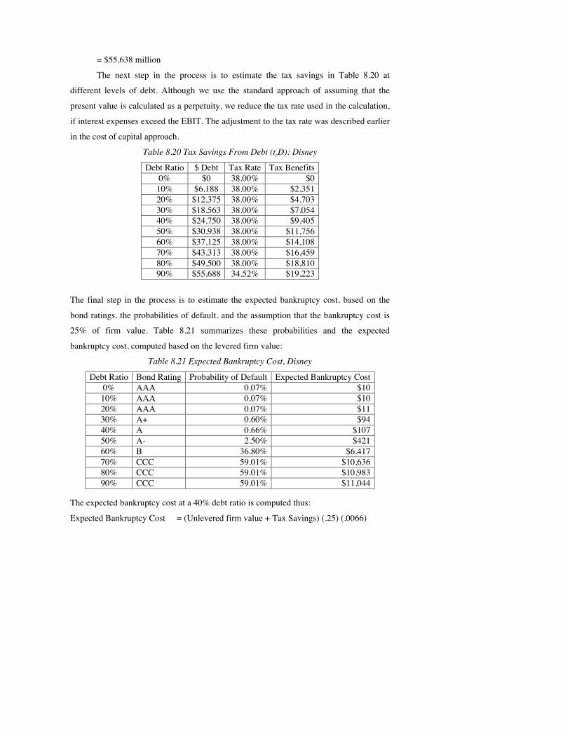
= $55,638 million
The next step in the process is to estimate the tax savings in Table 8.20 at
different levels of debt. Although we use the standard approach of assuming that the
present value is calculated as a perpetuity, we reduce the tax rate used in the calculation,
if interest expenses exceed the EBIT. The adjustment to the tax rate was described earlier
in the cost of capital approach.
Table 8.20 Tax Savings From Debt (tcD): Disney
Debt Ratio $ Debt Tax Rate Tax Benefits 0% $0 38.00% $0 10% $6,188 38.00% $2,351 20% $12,375 38.00% $4,703 30% $18,563 38.00% $7,054 40% $24,750 38.00% $9,405 50% $30,938 38.00% $11,756 60% $37,125 38.00% $14,108 70% $43,313 38.00% $16,459 80% $49,500 38.00% $18,810 90% $55,688 34.52% $19,223
The final step in the process is to estimate the expected bankruptcy cost, based on the
bond ratings, the probabilities of default, and the assumption that the bankruptcy cost is
25% of firm value. Table 8.21 summarizes these probabilities and the expected
bankruptcy cost, computed based on the levered firm value:
Table 8.21 Expected Bankruptcy Cost, Disney
Debt Ratio Bond Rating Probability of Default Expected Bankruptcy Cost 0% AAA 0.07% $10
10% AAA 0.07% $10 20% AAA 0.07% $11 30% A+ 0.60% $94 40% A 0.66% $107 50% A- 2.50% $421 60% B 36.80% $6,417 70% CCC 59.01% $10,636 80% CCC 59.01% $10,983 90% CCC 59.01% $11,044
The expected bankruptcy cost at a 40% debt ratio is computed thus:
Expected Bankruptcy Cost = (Unlevered firm value + Tax Savings) (.25) (.0066)

= (55,638+$9,405) (.25) (0.0066) = $ 107 million
The value of the levered firm is estimated in Table 8.22 by aggregating the effects of the
tax savings and the expected bankruptcy costs.
Table 8.22 Value of Disney with Leverage
Debt Ratio $ Debt
Tax Rate
Unlevered Firm Value
Tax Benefits
Expected Bankruptcy
Cost
Value of Levered
Firm 0% $0 38.00% $55,638 $0 $10 $55,629 10% $6,188 38.00% $55,638 $2,351 $10 $57,979 20% $12,375 38.00% $55,638 $4,703 $11 $60,330 30% $18,563 38.00% $55,638 $7,054 $94 $62,598 40% $24,750 38.00% $55,638 $9,405 $107 $64,936 50% $30,938 38.00% $55,638 $11,756 $421 $66,973 60% $37,125 38.00% $55,638 $14,108 $6,417 $63,329 70% $43,313 38.00% $55,638 $16,459 $10,636 $61,461 80% $49,500 38.00% $55,638 $18,810 $10,983 $63,466 90% $55,688 34.52% $55,638 $19,223 $11,044 $63,817
The firm value is maximized at about 50% debt, slightly higher than the optimal
computed using the cost of capital approach. These results are, however, very sensitive to
both the estimate of bankruptcy cost as a percent of firm value and the probabilities of
default.
Benefits and Limitations of the APV Approach
The advantage of the APV approach is that it separates the effects of debt into
different components and allows an analyst to use different discount rates for each
component. In this approach, we do not assume that the debt ratio stays unchanged
forever, which is an implicit assumption in the cost of capital approach. Instead, we have
the flexibility to keep the dollar value of debt fixed and to calculate the benefits and costs
of the fixed dollar debt.
These advantages have to be weighed against the difficulty of estimating
probabilities of default and the cost of bankruptcy. In fact, many analyses that use the
APV approach ignore the expected bankruptcy costs, leading them to the conclusion that
firm value increases as firms borrow money. Not surprisingly, they conclude that the
optimal debt ratio for a firm is 100% debt.

In general, with the same assumptions, the APV and the cost of capital
conclusions give identical answers. However, the APV approach is more practical when
firms are evaluating the feasibility of adding a dollar amount of debt, whereas the cost of
capital approach is easier when firms are analyzing debt proportions.24
apv.xls: This spreadsheet allows you to compute the value of a firm, with leverage,
using the adjusted present value approach
Comparative Analysis The most common approach to analyzing the debt ratio of a firm is to compare its
leverage to that of similar firms. A simple way to perform this analysis is to compare a
firm's debt ratio to the average debt ratio for the industry in which the firm operates. A
more complete analysis would consider the differences between a firm and the rest of the
industry, when determining debt ratios. We will consider both ways below.
Comparing to Industry Average
Firms sometimes choose their financing mixes by looking at the average debt
ratio of other firms in the industry in which they operate. For instance, table 8.23
compares the debt ratios at Disney, Aracruz and Tata Chemicals to other firms in their
industries. We define these comparable firms as US entertainment companies for Disney,
emerging market paper companies for Aracruz and emerging market chemical companies
for Tata Chemicals.
Table 8.23: Comparison to Industry Averages
Book Debt Ratio Market Debt Ratio Company Book Debt
Ratio Market Debt Ratio
Comparable group Average Median Average Median
Disney 32.89% 26.96% US Entertainment companies
47.76% 43.59% 36.90% 37.83%
Aracruz 91.01% 52.47% Emerging Market Paper companies
38.11% 40.74% 33.75% 34.22%
Tata Chemicals
42.95% 34.02% Emerging Market chemical companies
33.88% 34.76% 25.56% 21.34%
Source: Value Line & Capital IQ.
24 Inselbag, I. and H. Kaufold, 1997, Two DCF Approaches and Valuing Companies under Alternative Financing Strategies, Journal of Applied Corporate Finance, v10(1), 115-122.
Based on this comparison, Disney is operating at a debt ratio lower than those of other
firms in the industry in both market and book value terms, whereas Aracruz and Tata
Chemicals have debt ratios much higher than the averages for their sector.
The underlying assumptions in this
comparison are that firms within the same industry
are comparable and that, on average, these firms are
operating at or close to their optimal. Both
assumptions can be questioned, however. Firms
within the same industry can have different product
mixes, different amounts of operating risk, different
tax rates, and different project returns. In fact, most
do. For instance, Disney is considered part of the
entertainment industry, but its mix of businesses is very different from that of Lion’s
Gate, which is primarily a movie company, or Liberty Media, which is primarily a cable
broadcasting company. Furthermore, Disney’s size and risk characteristics are very
different from that of Westwood One, which is also considered part of the same industry
group. The other problem is that, as we noted in Chapter 4, both Disney and Tata
Chemicals are multi-business companies and picking a sector to compare these firms is
difficult to do.
There is a data set online that summarizes market value and book value debt ratios,
by industry, in addition to other relevant characteristics.
Controlling for Differences between Firms
Firms within the same industry can exhibit wide differences on tax rates, capacity
to generate operating income and cash flows, and variance in operating income.
Consequently, it can be dangerous to compare a firm’s debt ratio to the industry and draw
conclusions about the optimal financing mix. The simplest way to control for differences
across firms, while using the maximum information available in the market, is to run a
regression, regressing debt ratios against these variables, across the firms in a industry:
Debt Ratio = α0 + α1 Tax Rate + α2 Pretax Returns + α3 Variance in Operating Income
Comparable (Firm): A firm similar
to the firm being analyzed in terms
of underlying characteristics—risk,
growth, and cash flow patterns. The
conventional definition of
comparable firm is one that is the
same business as the one being
analyzed and of similar size.
There are several advantages to the cross-sectional approach. Once the regression
has been run and the basic relationship established (i.e., the intercept and coefficients
have been estimated), the predicted debt ratio for any firm can be computed quickly using
the measures of the independent variables for this firm. If a task involves calculating the
optimal debt ratio for a large number of firms in a short time period, this may be the only
practical way of approaching the problem, because the other approaches described in this
chapter are time-intensive.
There are also limitations to this approach. The coefficients tend to shift over
time. Besides some standard statistical problems and errors in measuring the variables,
these regressions also tend to explain only a portion of the differences in debt ratios
between firms. However, the regressions provide significantly more information than a
naive comparison of a firm’s debt ratio to the industry average.
Sticking with Industry Averages: A Behavioral Perspective
The pull of industry averages on the debt ratios of individual firms in the industry
is too strong to be ignored. While it may make little sense from a fundamental standpoint
to mimic the behavior of other firms in the sector, there are two reasons that have been
offered for why it appeals to managers.
a. Herd migration: Patel, Zeckhauser and Hendricks (1991) use the behavior of birds
and wildebeest to explain why companies stick close to industry averages.25 They
note that the same “safety in numbers” that induces animals to travel in groups also
influences managers when they make financing choices. Put another way, a manager
who chooses to take on a significant amount of debt, simply because other firms in
the sector have also done so, is unlikely to be fired even if that debt turns out to be too
high, in hindsight. In fact, if analysts follow the same herd mentality, they are likely
to punish firms that deviate from the herd, even if that deviation can be justified on
intrinsic grounds. Looking across 182 firms in ten sectors, they find evidence of herd
behavior in seven of the ten sectors. 25 Patel,J.,R.Zeckhauser,andD.Hendricks,1991,“TheRationalityStruggle:IllustrationsfromFinancialMarkets,”AmericanEconomicReviewPapersandProceedings,pp.232‐236.AmericanEconomicReviewPapersandProceedings,1991,pp.232‐236.

b. Following the leader: A variant of this theme, with its roots in the natural sciences as
well, is that firms in a business tend to follow the leader. In this model, success and
reputation lead to a firm being anointed the leader for a sector. When this firm
chooses a financing mix, presumably based upon its fundamentals, other firms in that
sector then imitate the leader, hoping to imitate its success
Whatever the reasons may be, there is no denying the fact that managers look at industry
averages and practices on capital structure for guidance. Consequently, it does make
sense to check the optimal debt ratios that emerge from the cost of capital and APV
approaches against industry averages and to adjust them towards peer group ratios.
Illustration 8.9: Estimating Disney’s Debt Ratio Using the Cross-Sectional Approach
This approach can be applied to look at differences within an industry or across
the entire market. We can illustrate looking at the Disney against firms in the
entertainment sector first and then against the entire market.
To look at the determinants of debt ratios within the entertainment industry, we
regressed debt ratios of the 80 firms in the industry against two variables—the effective
tax rate and the EBITDA as a percent of the market value of the firm. Based on our
earlier discussion of the determinants of capital structure, we would expect firms with
higher operating cash flows (EBITDA) as a percent of firm value to borrow more money.
We would also expect higher tax rates to lead to more benefits from debt and higher debt
ratios. The results of the regression are reported, with t-statistics in brackets below the
coefficients:
Debt to Capital = 0.049 + 0.543 (Effective tax rate) + 0.692 (EBITDA/Firm Value)
(1.07) (4.10a) (4.08a)
The dependent variable is the market debt to capital ratio, and the regression has an R2 of
40%. Although there is statistical significance, it is worth noting that the predicted debt
ratios will have substantial standard errors associated with them. Even so, if we use the
current values for these variables for Disney in this regression, we get a predicted debt
ratio:
DFRDisney= 0.049 + 0.543 (0.372) + 0.692 (0.1735) = 0.3710 or 37.10%

At its existing debt ratio of 27%, Disney is significantly under levered. Thus, relative to
the industry in which it operates and its specific characteristics, Disney could potentially
borrow more.
One of the limitations of this analysis is that there are only a few firms within
each industry. This analysis can be extended to all firms in the market. Although firms in
different businesses differ in terms of risk and cash flows and these differences can
translate into differences in debt ratios, we can control for the differences in the
regression. To illustrate, we regressed debt ratios of all listed firms in the United States
against four variables:
• The expected growth rate in EPS (GEPS) as a proxy for growth assets. Firms with a
higher percentage of value from growth assets should have less debt.
• Closely held shares as a percent of shares outstanding (CLSH) as a measure of
how much separation there is between managers and stockholders (and hence as a
proxy for debt as a disciplinary mechanism).
• EBITDA as a percent of enterprise value (E/V) as a measure of the cash flow
generating capacity of a firm
• Intangible assets as a percentage of total assets (Intangible %); firms that derive
more of their value from intangible assets face bigger agency costs (with lenders)
and should borrow less.
The results of the regression from early 2009 are presented below.26
DFR = 0.327 - 0.064 Intangible % – 0.138 CLSH + 0.026 E/V – 0.878 GEPS
(25.45a) (2.16a) (2.88a) (1.25) (12.6a)
where DFR is debt as a percentage of the market value of the firm (debt + equity). The R2
for this regression is only 13%. If we plug in the values for Disney in 2009 into this
regression, we get a predicted debt ratio:
DFRDisney= 0.327 - 0.064 (0.24) – 0.138 (0.077) + 0.0.26 (0.1735) – 0.878 (0.065)
= 0.2891 or 28.91%
26 This regression has about 2000 publicly traded companies in the United States, with information available on both debt ratios and the independent variables.
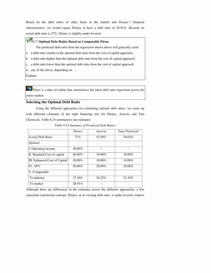
Based on the debt ratios of other firms in the market and Disney’s financial
characteristics, we would expect Disney to have a debt ratio of 28.91%. Because its
actual debt ratio is 27%, Disney is slightly under levered.
8.7. Optimal Debt Ratios Based on Comparable Firms
The predicted debt ratio from the regression shown above will generally yield
a. a debt ratio similar to the optimal debt ratio from the cost of capital approach.
b. a debt ratio higher than the optimal debt ratio from the cost of capital approach.
c. a debt ratio lower than the optimal debt ratio from the cost of capital approach.
d. any of the above, depending on . . .
Explain.
There is a data set online that summarizes the latest debt ratio regression across the
entire market.
Selecting the Optimal Debt Ratio Using the different approaches for estimating optimal debt ratios, we come up
with different estimates of the right financing mix for Disney, Aracruz and Tata
Chemicals. Table 8.24 summarizes our estimates:
Table 8.24 Summary of Predicted Debt Ratios
Disney Aracruz Tata Chemicals
Actual Debt Ratio 27% 52.58% 34.02%
Optimal
I. Operating income 50.00% — -
II. Standard Cost of capital 40.00% 10.00% 10.00%
III. Enhanced Cost of Capital 30.00% 10.00% 10.00%
IV. APV 50.00% 20.00% 10.00%
V. Comparable
To industry 37.10% 34.22% 21.34%
To market 28.91% — -
Although there are differences in the estimates across the different approaches, a few
consistent conclusions emerge: Disney, at its existing debt ratio, is under levered, relative

to every estimate of the optimal debt ratio, though it looks less under levered relative to
the rest of the market, than it does relative to its own fundamentals or to the sector.
Aracruz and Tata Chemicals are both over levered, relative to every estimate of the
optimal debt ratio.
With Bookscape, we will stick with the conclusion that we drew earlier, based
upon the cost of capital approach. The firm at its existing debt ratio is very close to its
optimal and has the right amount of debt.
Conclusion This chapter has provided background on four tools that can be used to analyze
capital structure.
• The first approach is based on operating income. Using historical data or forecasts,
we develop a distribution of operating income across both good and bad scenarios.
We then use a predefined acceptably probability of default to specify the maximum
borrowing capacity.
• The second approach is the cost of capital—the weighted average of the costs of
equity, debt, and preferred stock, where the weights are market value weights and the
costs of financing are current costs. The objective is to minimize the cost of capital,
which also maximizes the value of the firm. We also considered an enhanced version
of this approach, where the cash flows also change as the debt ratio changes, and the
optimal debt ratio is the one that delivers the highest firm value, rather than the lowest
cost of capital.
• The APV approach estimates the value of the firm at different levels of debt by
adding the present value of the tax benefits from debt to the unlevered firm’s value,
and then subtracting out the present value of expected bankruptcy costs. The optimal
debt ratio is the one that maximizes firm value.
• The final approach is to compare a firm’s debt ratio to similar firms. Although
comparisons of firm debt ratios to an industry average are commonly made, they are
generally not very useful in the presence of large differences among firms within the
same industry. A cross-sectional regression of debt ratios against underlying financial
variables brings in more information from the general population of firms and can be
used to predict debt ratios for a large number of firms.

The objective in all of these analyses is to come up with a mix of debt and equity that will
maximize the value of the firm.

Live Case Study
The Optimal Financing Mix
Objective: To estimate the optimal mix of debt and equity for your firm and to evaluate
the effect on firm value of moving to that mix.
Key Questions
• Based on the cost of capital approach, what is the optimal debt ratio for your firm?
Bringing in reasonable constraints into the decision process, what would your
recommended debt ratio be for this firm?
• Does your firm have too much or too little debt
- relative to the industry in which they operate?
- relative to the market?
Framework for Analysis
1. Cost of Capital Approach
• What is the current cost of capital for the firm?
• What happens to the cost of capital as the debt ratio is changed?
• At what debt ratio is the cost of capital minimized and firm value maximized?
(If they are different, explain.)
• What will happen to the firm value if the firm moves to its optimal?
• What will happen to the stock price if the firm moves to the optimal and
stockholders are rational?
2. Building Constraints into the Process
• What rating does the company have at the optimal debt ratio? If you were to
impose a rating constraint, what would it be? Why? What is the optimal debt
ratio with this rating constraint?
• How volatile is the operating income? What is the “normalized” operating
income of this firm, and what is the optimal debt ratio of the firm at this level
of income?
3. Relative Analysis
• Relative to the industry to which this firm belongs, does it have too much or
too little in debt? (Do a regression, if necessary.)

• Relative to the rest of the firms in the market, does it have too much or too
little in debt? (Use the market regression, if necessary.)
Getting Information about Optimal Capital Structure
To get the inputs needed to estimate the optimal capital structure, examine
regulatory filings and the annual report. The ratings and interest coverage ratios can be
obtained from the ratings agencies (S&P, Moody’s), and default spreads can be estimated
by finding traded bonds in each ratings class.
Online sources of information:
www.stern.nyu.edu/~adamodar/cfin2E/project/data.htm

Problems and Questions 1. Plastico, a manufacturer of consumer plastic products, is evaluating its capital
structure. The balance sheet of the company is as follows (in millions):
Assets Liabilities
Fixed assets $4,000 Debt $2,500
Current assets $1,000 Equity $2,500
In addition, you are provided the following information:
• The debt is in the form of long-term bonds, with a coupon rate of 10%. The bonds
are currently rated AA and are selling at a yield of 12% (the market value of the bonds is
80% of the face value).
• The firm currently has 50 million shares outstanding, and the current market price
is $80 per share. The firm pays a dividend of $4 per share and has a price/earnings ratio
of 10.
• The stock currently has a beta of 1.2. The six-month Treasury bill rate is 8%.
• The tax rate for this firm is 40%.
a. What is the debt/equity ratio for this firm in book value terms? In market value
terms?
b. What is the debt/(debt + equity) ratio for this firm in book value terms? In market
value terms?
c. What is the firm’s after-tax cost of debt?
d. What is the firm’s cost of equity?
e. What is the firm’s current cost of capital?
2. Now assume that Plastico is considering a project that requires an initial investment of
$100 million and has the following projected income statement (depreciation for the
project is expected to be $5 million a year forever.):
EBIT $20 million – Interest $4 million EBT $16 million Taxes $6.40 million Net income $9.60 million
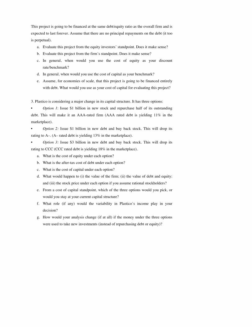
This project is going to be financed at the same debt/equity ratio as the overall firm and is
expected to last forever. Assume that there are no principal repayments on the debt (it too
is perpetual).
a. Evaluate this project from the equity investors’ standpoint. Does it make sense?
b. Evaluate this project from the firm’s standpoint. Does it make sense?
c. In general, when would you use the cost of equity as your discount
rate/benchmark?
d. In general, when would you use the cost of capital as your benchmark?
e. Assume, for economies of scale, that this project is going to be financed entirely
with debt. What would you use as your cost of capital for evaluating this project?
3. Plastico is considering a major change in its capital structure. It has three options:
• Option 1: Issue $1 billion in new stock and repurchase half of its outstanding
debt. This will make it an AAA-rated firm (AAA rated debt is yielding 11% in the
marketplace).
• Option 2: Issue $1 billion in new debt and buy back stock. This will drop its
rating to A–. (A– rated debt is yielding 13% in the marketplace).
• Option 3: Issue $3 billion in new debt and buy back stock. This will drop its
rating to CCC (CCC rated debt is yielding 18% in the marketplace).
a. What is the cost of equity under each option?
b. What is the after-tax cost of debt under each option?
c. What is the cost of capital under each option?
d. What would happen to (i) the value of the firm; (ii) the value of debt and equity;
and (iii) the stock price under each option if you assume rational stockholders?
e. From a cost of capital standpoint, which of the three options would you pick, or
would you stay at your current capital structure?
f. What role (if any) would the variability in Plastico’s income play in your
decision?
g. How would your analysis change (if at all) if the money under the three options
were used to take new investments (instead of repurchasing debt or equity)?

h. What other considerations (besides minimizing the cost of capital) would you
bring to bear on your decision?
i. Intuitively, why doesn’t the higher rating in option 1 translate into a lower cost of
capital?
4. Plastico is interested in how it compares with its competitors in the same industry.
Plastico Competitors
Debt/Equity Ratio 50% 25%
Variance in EBITDA 20% 40%
EBITDA/MV of firm 25% 15%
Tax rate 40% 30%
R&D/sales 2% 5%
a. Taking each of these variables, explain at an intuitive level whether you would
expect Plastico to have more or less debt than its competitors and why.
b. You have also run a regression of debt/equity ratios against these variables for all
the firms on the NYSE and have come up with the following regression equation:
D/E = 0.10 - 0.5 (Variance in EBITDA) + 2.0 (EBITDA/MV) + 0.4 (Tax Rate) +
2.5 (R&D/Sales)
(All inputs to the regression were in decimals, i.e., 20% was inputted as 0.20.)
Given this cross-sectional relationship, what would you expect Plastico’s
debt/equity ratio to be?
5. As CEO of a major corporation, you have to make a decision on how much you can
afford to borrow. You currently have 10 million shares outstanding, and the market price
per share is $50. You also currently have about $200 million in debt outstanding (market
value). You are rated as a BBB corporation now.
• Your stock has a beta of 1.5 and the six-month Treasure bill rate is 8%.
• Your marginal tax rate is 46%.
• You estimate that your rating will change to a B if you borrow $100 million. The
BBB rate now is 11%. The B rate is 12.5%.

a. Given the marginal costs and benefits of borrowing the $100 million, should you
go ahead with it ?
b. What is your best estimate of the weighted average cost of capital with and
without the $100 million in borrowing ?
c. If you borrow the $100 million, what will the price per share be after the
borrowing?
d. Assume that you have a project that requires an investment of $100 million. It has
expected before-tax revenues of $50 million and costs of $30 million a year in
perpetuity. Is this a desirable project by your criteria? Why or why not?
e. Does it make a difference in your decision if you were told that the cash flows
from the project in d are certain?
6. You have been hired as a management consultant by AD Corporation to evaluate
whether it has an appropriate amount of debt (the company is worried about a leveraged
buyout). You have collected the following information on AD’s current position:
• There are 100,000 shares outstanding at $20/share. The stock has a beta of 1.15.
• The company has $500,000 in long-term debt outstanding and is currently rated
BBB. The current market interest rate is 10% on BBB bonds and 6% on T-bills.
• The company’s marginal tax rate is 40%.
You proceed to collect the data on what increasing debt will do to the company’s ratings:
Additional Debt* New Rating Interest Rate
$500,000 BB 10.5
$1,000,000 B 11.5
$1,500,000 B– 13.5
$2,000,000 C 15
*In addition to the existing debt of $500,000.
a. How much additional debt should the company take on?
b.What will the price per share be after the company takes on new debt?
c. What is the WACC before and after the additional debt?
d.Assume that you are considering a project that has the following earnings in
perpetuity and is of comparable risk to existing projects.

Revenues/year $1,000,000
Cost of goods sold $400,000 (includes depreciation of
$100,000)
EBIT $600,000
Debt payments $100,000 (all interest payments)
Taxable Income $500,000
Tax $200,000
After-tax profit $300,000
If this project requires an investment of $3,000,000, what is its NPV?
7. UB is examining its capital structure with the intent of arriving at an optimal debt ratio.
It currently has no debt and has a beta of 1.5. The riskless interest rate is 9%. Your
research indicates that the debt rating will be as follows at different debt levels:
D/(D + E) Rating Interest Rate
0% AAA 10%
10% AA 10.5%
20% A 11%
30% BBB 12%
40% BB 13%
50% B 14%
60% CCC 16%
70% CC 18%
80% C 20%
90% D 25%
The firm currently has 1 million shares outstanding at $20 per share (tax rate = 40%).
a. What is the firm’s optimal debt ratio?
b. Assuming that the firm restructures by repurchasing stock with debt, what will the
value of the stock be after the restructuring?
8. GenCorp, an automotive parts manufacturer, currently has $25 million in outstanding debt and
has 10 million shares outstanding. The book value per share is $10, and the market value is $25.

The company is currently rated A, its bonds have a yield to maturity of 10%, and the current beta
of the stock is 1.06. The six-month T-bill rate is 8% now, and the company’s tax is 40%.
a. What is the company’s current weighted average cost of capital?
b. The company is considering a repurchase of 4 million shares at $25 per share with
new debt. It is estimated that this will push the company’s rating down to a B
(with a yield to maturity of 13%). What will the company’s WACC be after the
stock repurchase?
9. You have been called in as a consultant for Herbert’s a sporting goods retail firm, which is
examining its debt policy. The firm currently has a balance sheet as follows:
Liability Assets
LT Bonds $100 Fixed assets $300
Equity $300 Current assets $100
Total $400 Total $400
The firm’s income statement is as follows:
Revenues $250
Cost of Goods Sold (cogs) $175
Depreciation $25
EBIT $50
Long-term interest $10
EBT $40
Taxes $16
Net Income $24
The firm currently has 100 shares outstanding, selling at a market price of $5 per share and the
bonds are selling at par. The firm’s current beta is 1.12, and the six-month T-bill rate is 7%.
a. What is the firm’s current cost of equity?
b. What is the firm’s current cost of debt?
c. What is the firm’s current weighted average cost of capital?
a. Assume that management of Herbert’s is considering doing a debt-equity swap (i.e.,
borrowing enough money to buy back seventy shares of stock at $5 per share). It is

believed that this swap will lower the firm’s rating to C and raise the interest rate on the
company’s debt to 15%.
d. What is the firm’s new cost of equity?
e. What is the effective tax rate (for calculating the after-tax cost of debt) after the swap?
f. What is the firm’s new cost of capital?
10. Terck, a leading pharmaceutical company, currently has a balance sheet that is as follows:
Liability Assets
Long-term bonds $1.000 Fixed assets $1,700
Equity $1.000 Current assets $300
Total $1.000 Total $1,000
The firm’s income statement looks as follows:
Revenues $1,000
Cost of Goods Sold (COGS) $400
Depreciation $100
EBIT $500
Long-term interest expense $100
EBT $400
Taxes $200
Net income $200
The firm’s bonds are all twenty-year bonds with a coupon rate of 10% that are selling at 90% of
face value (the yield to maturity on these bonds is 11%). The stocks are selling at a P/E ratio of 9
and have a beta of 1.25. The six-month T-bill rate is 6%.
a. What is the firm’s current cost of equity?
b. What is the firm’s current after-tax cost of debt?
c. What is the firm’s current weighted average cost of capital?
Assume that management of Terck, which is very conservative, is considering doing an equity-
for-debt swap (i.e., issuing $200 more of equity to retire $200 of debt). This action is expected to
lower the firm's interest rate by 1%.
d. What is the firm’s new cost of equity?
e. What is the new WACC?

f. What will the value of the firm be after the swap?
11. You have been asked to analyze the capital structure of DASA, an environmental waste
disposal firm, and make recommendations on a future course of action. DASA has 40 million
shares outstanding, selling at $20 per share, and a debt/equity ratio (in market value terms) of
0.25. The beta of the stock is 1.15, and the firm currently has a AA rating, with a corresponding
market interest rate of 10%. The firm’s income statement is as follows:
EBIT $150 million
Interest expenses $20 million
Taxable income $130 million
Taxes $52 million
Net income $78 million
The current T-bill rate is 8%.
a. What is the firm’s current WACC?
b. The firm is proposing borrowing an additional $200 million in debt and
repurchasing stock. If it does so, its rating will decline to A, with a market interest
rate of 11%. What will the WACC be if they make this move?
c. What will the new stock price be if the firm borrows $200 million and
repurchases stock (assuming rational investors)?
d. Now assume that the firm has another option to raise its debt/equity ratio (instead
of borrowing money and repurchasing stock). It has considerable capital
expenditures planned for the next year ($150 million). The company also
currently pays $1 in dividends per share. If the company finances all its capital
expenditures with debt and doubles its dividend yield from the current level for
the next year, what would you expect the debt/equity ratio to be at the end of the
next year?
12. You have been asked by JJ Corporation, a California-based firm that manufacturers
and services digital satellite TV systems, to evaluate its capital structure. They currently
have 70 million shares outstanding trading at $10 per share. In addition, the company has
500,000 convertible bonds, with a coupon rate of 8%, trading at $1000 per bond. JJ is

rated BBB and the interest rate on BBB straight bonds is currently 10%. The beta for the
company is 1.2, and the current risk-free rate is 6%. The tax rate is 40%.
a. What is the firm’s current debt/equity ratio?
b. What is the firm’s current weighted average cost of capital?
JJ Corporation is proposing to borrow $250 million and use it for the following purposes:
• Buy back $100 million worth of stock.
• Pay $100 million in dividends.
• Invest $50 million in a project with a NPV of $25 million.
The effect of this additional borrowing will be a drop in the bond rating to B, which
currently carries an interest rate of 11%.
c. What will the firm’s cost of equity be after this additional borrowing?
d. What will the firm’s weighted average cost of capital be after this additional
borrowing?
e. What will the value of the firm be after this additional borrowing?

13. Pfizer, one of the largest pharmaceutical companies in the United States, is
considering what its debt capacity is. In March 1995, Pfizer had an outstanding market
value of equity of $24.27 billion, debt of $2.8 billion, and a AAA rating. Its beta was
1.47, and it faced a marginal corporate tax rate of 40%. The Treasury bond rate at the
time of the analysis was 6.50%, and AAA bonds trade at a spread of 0.30% over the
treasury rate.
a. Estimate the current cost of capital for Pfizer.
b. It is estimated that Pfizer will have a BBB rating if it moves to a 30% debt ratio
and that BBB bonds have a spread of 2% over the Treasury rate. Estimate the cost
of capital if Pfizer moves to its optimal.
c. Assuming a constant growth rate of 6% in the firm value, how much will firm
value change if Pfizer moves its optimal? What will the effect be on the stock
price?
d. Pfizer has considerable R&D expenses. Will this fact affect whether Pfizer takes
on the additional debt?
14. Upjohn, another major pharmaceutical company, is also considering whether it should
borrow more. It has $664 million in book value of debt outstanding and 173 million
shares outstanding at $30.75 per share. The company has a beta of 1.17, and faces a tax
rate of 36%. The Treasury bond rate is 6.50%.
a. If the interest expense on the debt is $55 million, the debt has an average maturity
of ten years, and the company is currently rated AA– (with a market interest rate
of 7.50%), estimate the market value of the debt.
b. Estimate the current cost of capital.
c. It is estimated that if Upjohn moves to its optimal debt ratio, and no growth in
firm value is assumed, the value per share will increase by $1.25. Estimate the
cost of capital at the optimal debt ratio.
15. Bethlehem Steel, one of the oldest and largest steel companies in the United States, is
considering the question of whether it has any excess debt capacity. The firm has $527
million in market value of debt outstanding and $1.76 billion in market value of equity.
The firm has earnings before interest and taxes of $131 million and faces a corporate tax

rate of 36%. The company’s bonds are rated BBB, and the cost of debt is 8%. At this
rating, the firm has a probability of default of 2.30%, and the cost of bankruptcy is
expected to be 30% of firm value.
a. Estimate the unlevered value of the firm.
b. Estimate the levered value of the firm, using the APV approach, at a debt ratio of
50%. At that debt ratio, the firm’s bond rating will be CCC, and the probability of
default will increase to 46.61%.
16. Kansas City Southern, a railroad company, had debt outstanding of $985 million and
40 million shares trading at $46.25 per share in March 1995. It earned $203 million in
EBIT, and faced a marginal tax rate of 36.56%. The firm was interested in estimating its
optimal leverage using the APV approach. The following table summarizes the estimated
bond ratings and probabilities of default at each level of debt from 0% to 90%.
Debt Ratio Bond Rating Probability of Default 0% AAA 0.28%
10% AAA 0.28% 20% A– 1.41% 30% BB 12.20% 40% B– 32.50% 50% CCC 46.61% 60% CC 65.00% 70% C 80.00% 80% C 80.00% 90% D 100.00%
The direct and indirect bankruptcy costs are estimated to be 25% of the firm value.
Estimate the optimal debt ratio of the firm, based on levered firm value.
17. In 1995, an analysis of the capital structure of Reebok provided the following results
on the cost of capital and firm value.
Actual Optimal Change
Debt ratio 4.42% 60.00% 55.58%
Beta for the stock 1.95 3.69 1.74
Cost of equity 18.61% 28.16% 9.56%
Bond rating A– B+
After-tax cost of debt 5.92% 6.87% 0.95%

Cost of capital 18.04% 15.38% –2.66%
Firm value (with no
growth)
$3,343 million $3,921 million $578 million
Stock price $39.50 $46.64 $7.14
This analysis was based on the 1995 EBIT of $420 million and a tax rate of 36.90%.
a. Why is the optimal debt ratio for Reebok so high?
b. What might be some of your concerns in moving to this optimal?
18. You are trying to evaluate whether United Airlines (UAL) has any excess debt
capacity. In 1995, UAL had 12.2 million shares outstanding at $210 per share and debt
outstanding of approximately $3 billion (book as well as market value). The debt had a
rating of B, and carried a market interest rate of 10.12%. In addition, the firm had leases
outstanding, with annual lease payments anticipated to by $150 million. The beta of the
stock is 1.26, and the firm faces a tax rate of 35%. The treasury bond rate is 6.12%.
a. Estimate the current debt ratio for UAL.
b. Estimate the current cost of capital.
c. Based on 1995 operating income, the optimal debt ratio is computed to be 30%, at
which point the rating will be BBB, and the market interest rate is 8.12%.
d. Would the fact that 1995 operating income for airlines was depressed alter your
analysis in any way? Explain why.
19. Intel has an EBIT of $3.4 billion and faces a marginal tax rate of 36.50%. It currently
has $1.5 billion in debt outstanding, and a market value of equity of $51 billion. The beta
for the stock is 1.35, and the pretax cost of debt is 6.80%. The Treasury bond rate is 6%.
Assume that the firm is considering a massive increase in leverage to a 70% debt ratio, at
which level the bond rating will be C (with a pretax interest rate of 16%).
a. Estimate the current cost of capital.
b. Assuming that all debt gets refinanced at the new market interest rate, what would
your interest expenses be at 70% debt? Would you be able to get the entire tax
benefit? Why or why not?

c. Estimate the beta of the stock at 70% debt, using the conventional levered beta
calculation. Reestimate the beta, on the assumption that C rated debt has a beta of
0.60. Which one would you use in your cost of capital calculation?
d. Estimate the cost of capital at 70% debt.
e. What will happen to firm value if Intel moves to a 70% debt ratio?
f. What general lessons on capital structure would you draw for other growth firms?
20. NYNEX, the phone utility for the New York City area, has approached you for advice
on its capital structure. In 1995, NYNEX had debt outstanding of $12.14 billion and
equity outstanding of $20.55 billion. The firm had an EBIT of $1.7 billion and faced a
corporate tax rate of 36%. The beta for the stock is 0.84, and the bonds are rated A– (with
a market interest rate of 7.5%). The probability of default for A– rated bonds is 1.41%,
and the bankruptcy cost is estimated to be 30% of firm value.
a. Estimate the unlevered value of the firm.
b. Value the firm, if it increases its leverage to 50%. At that debt ratio, its bond
rating would be BBB and the probability of default would be 2.30%.
c. Assume now that NYNEX is considering a move into entertainment, which is
likely to be both more profitable and riskier than the phone business. What
changes would you expect in the optimal leverage?
21. A small, private firm has approached you for advice on its capital structure decision.
It is in the specialty retailing business, and it had an EBIT last year of $500,000.
• The book value of equity is $1.5 million, but the estimated market value is $6 million.
• The firm has $1 million in debt outstanding and paid an interest expense of $80,000
on the debt last year. (Based on the interest coverage ratio, the firm would be rated
AA, and would be facing an interest rate of 8.25%.)
• The equity is not traded, but the average beta for comparable traded firms is 1.05, and
their average debt/equity ratio is 25%.
a. Estimate the current cost of capital for this firm.
b. Assume now that this firm doubles it debt from $1 million to $2 million and that
the interest rate at which it can borrow increases to 9%. Estimate the new cost of
capital and the effect on firm value.

c. You also have a regression that you have run of debt ratios of publicly traded
firms against firm characteristics:
DBTFR = 0.15 + 1.05 (EBIT/Firm Value) – 0.10 (Beta)
Estimate the debt ratio for the private firm, based on this regression.
d. What are some of the concerns you might have in extending the approaches used
by large publicly traded firms to estimate optimal leverage to smaller firms?
e. 22. XCV Inc., which manufactures automobile parts for assembly, is considering
the costs and the benefits of leverage. The CFO notes that the return on equity of
the firm, which is only 12.75% now based on the current policy of no leverage,
could be increased substantially by borrowing money. Is this true? Does it follow
that the value of the firm will increase with leverage? Why or why not?


