Chapter ML:III
III. Decision Treesq Decision Trees Basicsq Impurity Functionsq Decision Tree Algorithmsq Decision Tree Pruning
ML:III-67 Decision Trees © STEIN/LETTMANN 2005-2017

Decision Tree AlgorithmsID3 Algorithm [Quinlan 1986] [CART Algorithm]
Characterization of the model (model world) [ML Introduction] :
q X is a set of feature vectors, also called feature space.
q C is a set of classes.
q c : X → C is the ideal classifier for X.
q D = {(x1, c(x1)), . . . , (xn, c(xn))} ⊆ X × C is a set of examples.
Task: Based on D, construction of a decision tree T to approximate c.
ML:III-68 Decision Trees © STEIN/LETTMANN 2005-2017

Decision Tree AlgorithmsID3 Algorithm [Quinlan 1986] [CART Algorithm]
Characterization of the model (model world) [ML Introduction] :
q X is a set of feature vectors, also called feature space.
q C is a set of classes.
q c : X → C is the ideal classifier for X.
q D = {(x1, c(x1)), . . . , (xn, c(xn))} ⊆ X × C is a set of examples.
Task: Based on D, construction of a decision tree T to approximate c.
Characteristics of the ID3 algorithm:
1. Each splitting is based on one nominal feature and considers its completedomain. Splitting based on feature A with domain {a1, . . . , ak} :
X = {x ∈ X : x|A = a1} ∪ . . . ∪ {x ∈ X : x|A = ak}
2. Splitting criterion is the information gain.
ML:III-69 Decision Trees © STEIN/LETTMANN 2005-2017
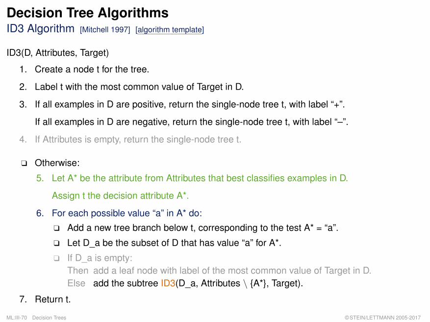
Decision Tree AlgorithmsID3 Algorithm [Mitchell 1997] [algorithm template]
ID3(D, Attributes, Target)
1. Create a node t for the tree.
2. Label t with the most common value of Target in D.
3. If all examples in D are positive, return the single-node tree t, with label “+”.
If all examples in D are negative, return the single-node tree t, with label “–”.
4. If Attributes is empty, return the single-node tree t.
q Otherwise:
5. Let A* be the attribute from Attributes that best classifies examples in D.
Assign t the decision attribute A*.
6. For each possible value “a” in A* do:
q Add a new tree branch below t, corresponding to the test A* = “a”.
q Let D_a be the subset of D that has value “a” for A*.
q If D_a is empty:Then add a leaf node with label of the most common value of Target in D.Else add the subtree ID3(D_a, Attributes \ {A*}, Target).
7. Return t.
ML:III-70 Decision Trees © STEIN/LETTMANN 2005-2017

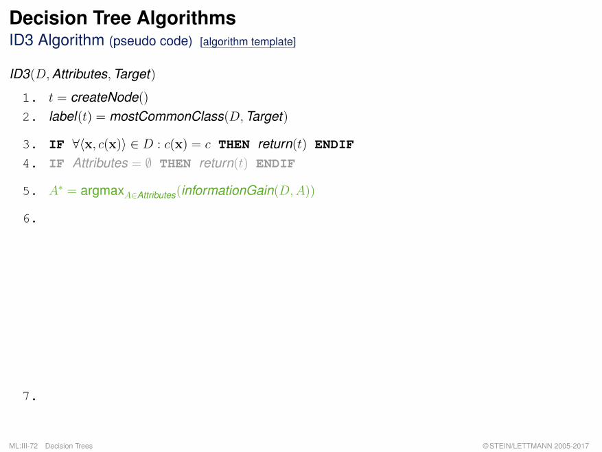
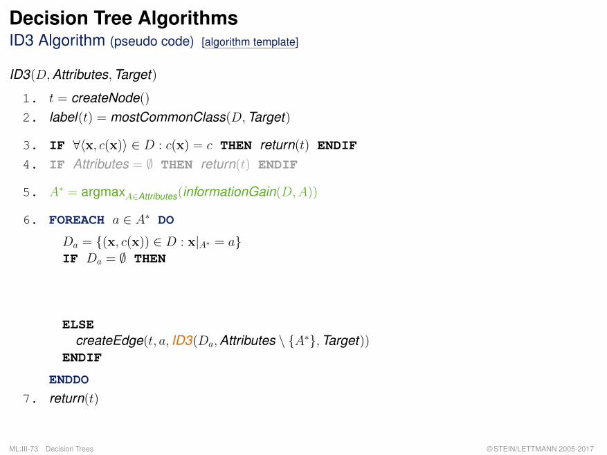
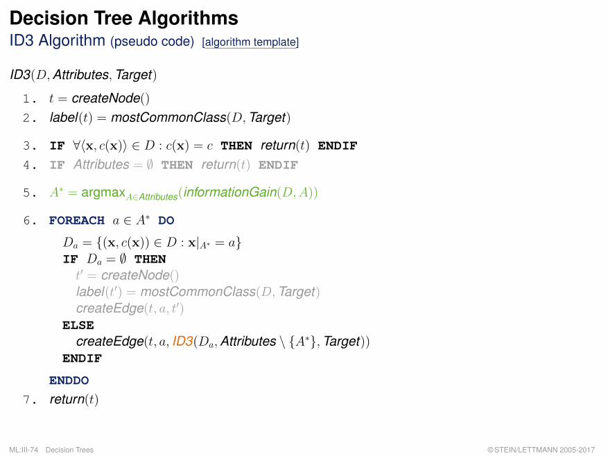
Decision Tree AlgorithmsID3 Algorithm (pseudo code) [algorithm template]
ID3(D,Attributes,Target)
1. t = createNode()2. label(t) = mostCommonClass(D,Target)
3. IF ∀〈x, c(x)〉 ∈ D : c(x) = c THEN return(t) ENDIF
4. IF Attributes = ∅ THEN return(t) ENDIF
5. A∗ = argmaxA∈Attributes(informationGain(D,A))
6. FOREACH a ∈ A∗ DO
Da = {(x, c(x)) ∈ D : x|A∗ = a}IF Da = ∅ THENt′ = createNode()label(t′) = mostCommonClass(D,Target)createEdge(t, a, t′)
ELSEcreateEdge(t, a, ID3(Da,Attributes \ {A∗},Target))
ENDIF
ENDDO
7. return(t)
ML:III-71 Decision Trees © STEIN/LETTMANN 2005-2017
Decision Tree AlgorithmsID3 Algorithm (pseudo code) [algorithm template]
ID3(D,Attributes,Target)
1. t = createNode()2. label(t) = mostCommonClass(D,Target)
3. IF ∀〈x, c(x)〉 ∈ D : c(x) = c THEN return(t) ENDIF
4. IF Attributes = ∅ THEN return(t) ENDIF
5. A∗ = argmaxA∈Attributes(informationGain(D,A))
6. FOREACH a ∈ A∗ DO
Da = {(x, c(x)) ∈ D : x|A∗ = a}IF Da = ∅ THENt′ = createNode()label(t′) = mostCommonClass(D,Target)createEdge(t, a, t′)
ELSEcreateEdge(t, a, ID3(Da,Attributes \ {A∗},Target))
ENDIF
ENDDO
7. return(t)
ML:III-72 Decision Trees © STEIN/LETTMANN 2005-2017
Decision Tree AlgorithmsID3 Algorithm (pseudo code) [algorithm template]
ID3(D,Attributes,Target)
1. t = createNode()2. label(t) = mostCommonClass(D,Target)
3. IF ∀〈x, c(x)〉 ∈ D : c(x) = c THEN return(t) ENDIF
4. IF Attributes = ∅ THEN return(t) ENDIF
5. A∗ = argmaxA∈Attributes(informationGain(D,A))
6. FOREACH a ∈ A∗ DO
Da = {(x, c(x)) ∈ D : x|A∗ = a}IF Da = ∅ THENt′ = createNode()label(t′) = mostCommonClass(D,Target)createEdge(t, a, t′)
ELSEcreateEdge(t, a, ID3(Da,Attributes \ {A∗},Target))
ENDIF
ENDDO
7. return(t)
ML:III-73 Decision Trees © STEIN/LETTMANN 2005-2017
Decision Tree AlgorithmsID3 Algorithm (pseudo code) [algorithm template]
ID3(D,Attributes,Target)
1. t = createNode()2. label(t) = mostCommonClass(D,Target)
3. IF ∀〈x, c(x)〉 ∈ D : c(x) = c THEN return(t) ENDIF
4. IF Attributes = ∅ THEN return(t) ENDIF
5. A∗ = argmaxA∈Attributes(informationGain(D,A))
6. FOREACH a ∈ A∗ DO
Da = {(x, c(x)) ∈ D : x|A∗ = a}IF Da = ∅ THENt′ = createNode()label(t′) = mostCommonClass(D,Target)createEdge(t, a, t′)
ELSEcreateEdge(t, a, ID3(Da,Attributes \ {A∗},Target))
ENDIF
ENDDO
7. return(t)
ML:III-74 Decision Trees © STEIN/LETTMANN 2005-2017
Remarks:
q “Target” designates the feature (= attribute) that is comprised of the labels according to whichan example can be classified. Within Mitchell’s algorithm the respective class labels are ‘+’and ‘–’, modeling the binary classification situation. In the pseudo code version, Target maycontain multiple (more than two) classes.
q Step 3 of of the ID3 algorithm checks the purity of D and, given this case, assigns the uniqueclass c, c ∈ dom(Target), as label to the respective node.
ML:III-75 Decision Trees © STEIN/LETTMANN 2005-2017
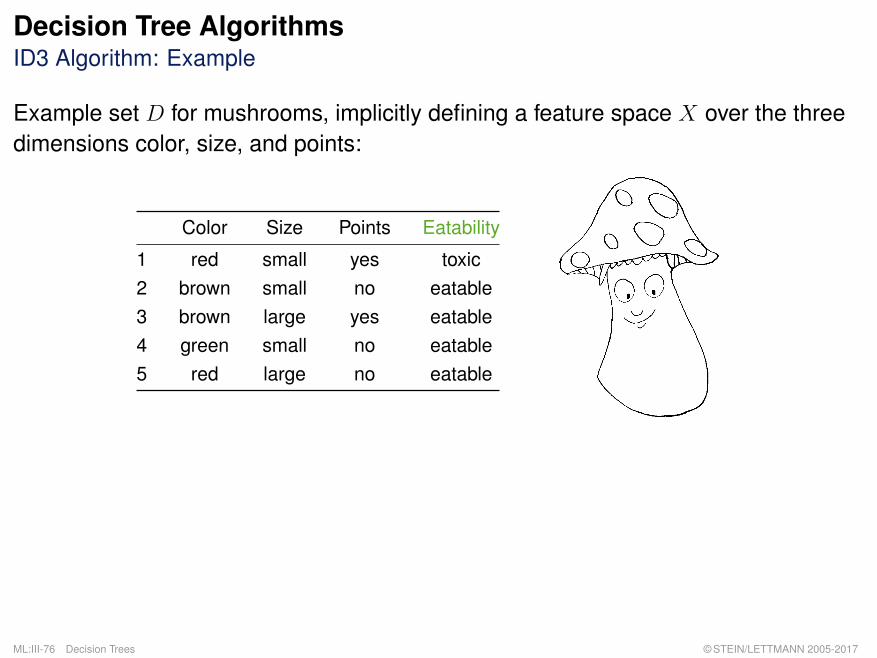
Decision Tree AlgorithmsID3 Algorithm: Example
Example set D for mushrooms, implicitly defining a feature space X over the threedimensions color, size, and points:
Color Size Points Eatability
1 red small yes toxic2 brown small no eatable3 brown large yes eatable4 green small no eatable5 red large no eatable
ML:III-76 Decision Trees © STEIN/LETTMANN 2005-2017

Decision Tree AlgorithmsID3 Algorithm: Example (continued)
Top-level call of ID3. Analyze a splitting with regard to the feature “color” :
D|color =
toxic eatablered 1 1brown 0 2green 0 1
Ü |Dred| = 2, |Dbrown| = 2, |Dgreen| = 1
Estimated a-priori probabilities:
pred =2
5= 0.4, pbrown =
2
5= 0.4, pgreen =
1
5= 0.2
ML:III-77 Decision Trees © STEIN/LETTMANN 2005-2017

Decision Tree AlgorithmsID3 Algorithm: Example (continued)
Top-level call of ID3. Analyze a splitting with regard to the feature “color” :
D|color =
toxic eatablered 1 1brown 0 2green 0 1
Ü |Dred| = 2, |Dbrown| = 2, |Dgreen| = 1
Estimated a-priori probabilities:
pred =2
5= 0.4, pbrown =
2
5= 0.4, pgreen =
1
5= 0.2
Conditional entropy values for all attributes:
H(C | color) = −(0.4 · (12 log212 +
12 log2
12) +
0.4 · (02 log202 +
22 log2
22) +
0.2 · (01 log201 +
11 log2
11)) = 0.4
H(C | size) ≈ 0.55
H(C | points) = 0.4
ML:III-78 Decision Trees © STEIN/LETTMANN 2005-2017
Remarks:
q The smaller H(C | feature) is, the larger becomes the information gain. Hence, the differenceH(C)−H(C | feature) needs not to be computed since H(C) is constant within eachrecursion step.
q In the example, the information gain in the first recursion step is maximum for the two features“color” and “points”.
ML:III-79 Decision Trees © STEIN/LETTMANN 2005-2017
Decision Tree AlgorithmsID3 Algorithm: Example (continued)
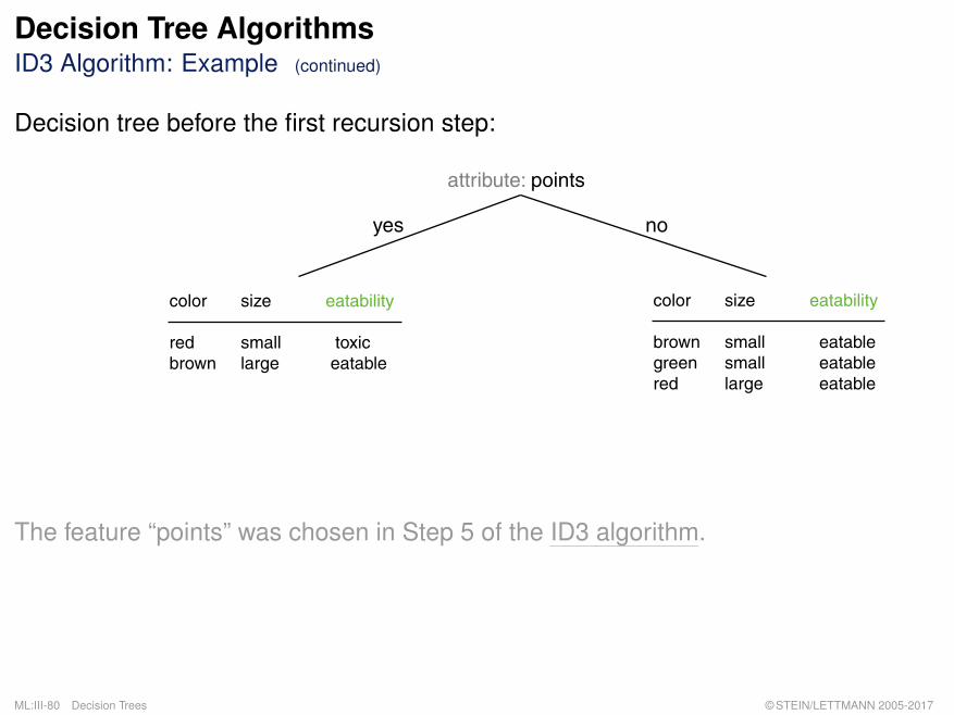
Decision tree before the first recursion step:
attribute: points
yes no
color size eatability
red small toxicbrown large eatable
color size eatability
brown small eatablegreen small eatablered large eatable
The feature “points” was chosen in Step 5 of the ID3 algorithm.
ML:III-80 Decision Trees © STEIN/LETTMANN 2005-2017
Decision Tree AlgorithmsID3 Algorithm: Example (continued)
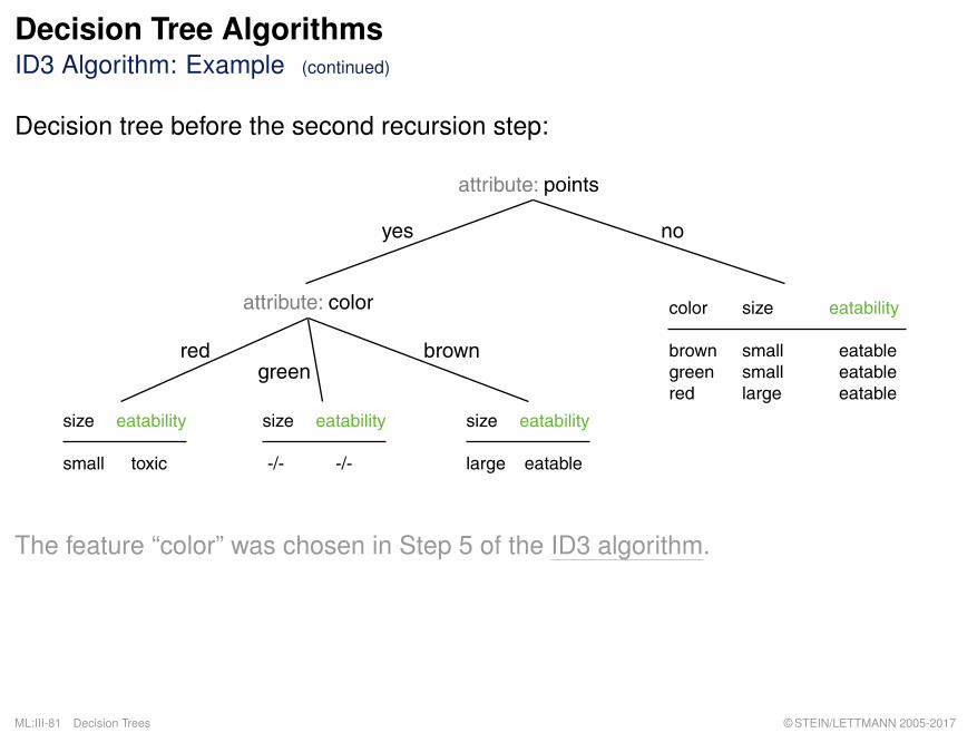
Decision tree before the second recursion step:
attribute: points
yes no
size eatability
small toxic
size eatability
large eatable
size eatability
-/- -/-
attribute: color
red browngreen
color size eatability
brown small eatablegreen small eatablered large eatable
The feature “color” was chosen in Step 5 of the ID3 algorithm.
ML:III-81 Decision Trees © STEIN/LETTMANN 2005-2017
Decision Tree AlgorithmsID3 Algorithm: Example (continued)
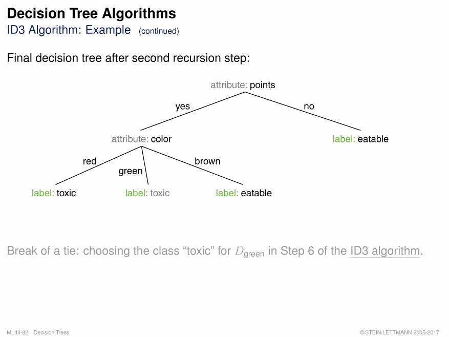
Final decision tree after second recursion step:
attribute: points
yes no
label: eatableattribute: color
red browngreen
label: toxic label: eatablelabel: toxic
Break of a tie: choosing the class “toxic” for Dgreen in Step 6 of the ID3 algorithm.
ML:III-82 Decision Trees © STEIN/LETTMANN 2005-2017

Decision Tree AlgorithmsID3 Algorithm: Hypothesis Space
+ +-
o
+ +- o +o
A1
+ +- o -
A2
+ +-
+ o
-
A2
A3 + +-
o -
-
A2
A4
...
... ...
...
...
ML:III-83 Decision Trees © STEIN/LETTMANN 2005-2017
Decision Tree AlgorithmsID3 Algorithm: Inductive Bias
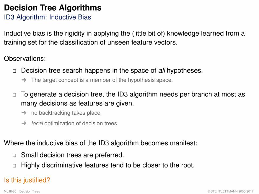
Inductive bias is the rigidity in applying the (little bit of) knowledge learned from atraining set for the classification of unseen feature vectors.
Observations:
q Decision tree search happens in the space of all hypotheses.The target concept is a member of the hypothesis space.
q To generate a decision tree, the ID3 algorithm needs per branch at most asmany decisions as features are given.
no backtracking takes place
local optimization of decision trees
ML:III-84 Decision Trees © STEIN/LETTMANN 2005-2017

Decision Tree AlgorithmsID3 Algorithm: Inductive Bias
Inductive bias is the rigidity in applying the (little bit of) knowledge learned from atraining set for the classification of unseen feature vectors.
Observations:
q Decision tree search happens in the space of all hypotheses.Ü The target concept is a member of the hypothesis space.
q To generate a decision tree, the ID3 algorithm needs per branch at most asmany decisions as features are given.Ü no backtracking takes place
Ü local optimization of decision trees
ML:III-85 Decision Trees © STEIN/LETTMANN 2005-2017
Decision Tree AlgorithmsID3 Algorithm: Inductive Bias
Inductive bias is the rigidity in applying the (little bit of) knowledge learned from atraining set for the classification of unseen feature vectors.
Observations:
q Decision tree search happens in the space of all hypotheses.Ü The target concept is a member of the hypothesis space.
q To generate a decision tree, the ID3 algorithm needs per branch at most asmany decisions as features are given.Ü no backtracking takes place
Ü local optimization of decision trees
Where the inductive bias of the ID3 algorithm becomes manifest:
q Small decision trees are preferred.q Highly discriminative features tend to be closer to the root.
Is this justified?ML:III-86 Decision Trees © STEIN/LETTMANN 2005-2017
Remarks:
q Let Aj be the finite domain (the possible values) of feature Aj, j = 1, . . . , p, and let C be a setof classes. Then, a hypothesis space H that is comprised of all decision trees corresponds tothe set of all functions h, h : A1 × . . .×Ap → C. Typically, C = {0, 1}.
q The inductive bias of the ID3 algorithm is of a different kind than the inductive bias of thecandidate elimination algorithm (version space algorithm):
1. The underlying hypothesis space H of the candidate elimination algorithm is incomplete.H corresponds to a coarsened view onto the space of all hypotheses since H containsonly conjunctions of attribute-value pairs as hypotheses. However, this restrictedhypothesis space is searched completely by the candidate elimination algorithm.Keyword: restriction bias
2. The underlying hypothesis space H of the ID3 algorithm is complete. H corresponds tothe set of all discrete functions (from the Cartesian product of the feature domains ontothe set of classes) that can be represented in the form of a decision tree. However, thiscomplete hypothesis space is searched incompletely (following a preference).Keyword: preference bias or search bias
q The inductive bias of the ID3 algorithm renders the algorithm robust with respect to noise.
ML:III-87 Decision Trees © STEIN/LETTMANN 2005-2017
Decision Tree AlgorithmsCART Algorithm [Breiman 1984] [ID3 Algorithm]
Characterization of the model (model world) [ML Introduction] :
q X is a set of feature vectors, also called feature space.No restrictions are presumed for the features’ measurement scales.
q C is a set of classes.
q c : X → C is the ideal classifier for X.
q D = {(x1, c(x1)), . . . , (xn, c(xn))} ⊆ X × C is a set of examples.
Task: Based on D, construction of a decision tree T to approximate c.
ML:III-88 Decision Trees © STEIN/LETTMANN 2005-2017

Decision Tree AlgorithmsCART Algorithm [Breiman 1984] [ID3 Algorithm]
Characterization of the model (model world) [ML Introduction] :
q X is a set of feature vectors, also called feature space.No restrictions are presumed for the features’ measurement scales.
q C is a set of classes.
q c : X → C is the ideal classifier for X.
q D = {(x1, c(x1)), . . . , (xn, c(xn))} ⊆ X × C is a set of examples.
Task: Based on D, construction of a decision tree T to approximate c.
Characteristics of the CART algorithm:
1. Each splitting is binary and considers one feature at a time.
2. Splitting criterion is the information gain or the Gini index.
ML:III-89 Decision Trees © STEIN/LETTMANN 2005-2017
Decision Tree AlgorithmsCART Algorithm (continued)
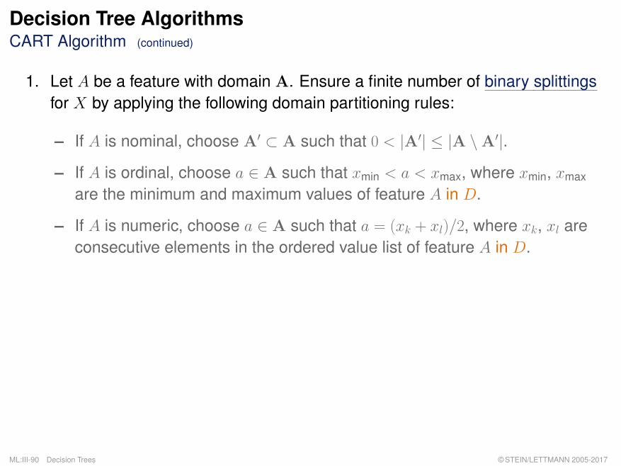
1. Let A be a feature with domain A. Ensure a finite number of binary splittingsfor X by applying the following domain partitioning rules:
– If A is nominal, choose A′ ⊂ A such that 0 < |A′| ≤ |A \A′|.
– If A is ordinal, choose a ∈ A such that xmin < a < xmax, where xmin, xmax
are the minimum and maximum values of feature A in D.
– If A is numeric, choose a ∈ A such that a = (xk + xl)/2, where xk, xl areconsecutive elements in the ordered value list of feature A in D.
ML:III-90 Decision Trees © STEIN/LETTMANN 2005-2017

Decision Tree AlgorithmsCART Algorithm (continued)
1. Let A be a feature with domain A. Ensure a finite number of binary splittingsfor X by applying the following domain partitioning rules:
– If A is nominal, choose A′ ⊂ A such that 0 < |A′| ≤ |A \A′|.
– If A is ordinal, choose a ∈ A such that xmin < a < xmax, where xmin, xmax
are the minimum and maximum values of feature A in D.
– If A is numeric, choose a ∈ A such that a = (xk + xl)/2, where xk, xl areconsecutive elements in the ordered value list of feature A in D.
2. For node t of a decision tree generate all splittings of the above type.
3. Choose a splitting from the set of splittings that maximizes the impurityreduction ∆ι :
∆ι(D(t), {D(tL), D(tR)}) = ι(t)− |DL||D|· ι(tL)− |DR|
|D|· ι(tR),
where tL and tR denote the left and right successor of t.
ML:III-91 Decision Trees © STEIN/LETTMANN 2005-2017

Decision Tree AlgorithmsCART Algorithm (continued)
Illustration for two numeric features, i.e., the feature space X corresponds to atwo-dimensional plane:
t1
t3t2 X(t2)
c1
c2c3
c3
c1
X(t3)
t5t4 X(t5)X(t4)
X(t1)
X(t6)t6
X(t6)
X(t9)
X(t7)
X(t8)
X(t4)
X(t9)
X(t7)
X(t8)
X = X(t1)
By a sequence of splittings the feature space X is partitioned into rectangles thatare parallel to the two axes.
ML:III-92 Decision Trees © STEIN/LETTMANN 2005-2017


