
Characterization and Modeling of Land Subsidence due to Groundwater Withdrawals
from the Confined Aquifers of the Virginia Coastal Plain
Jason P. Pope
Thesis submitted to the Faculty of the Virginia Polytechnic Institute and State University
in partial fulfillment for the requirements for the degree of
Master of Science in
Geological Sciences
Thomas J. Burbey, Chair George E. Harlow, Jr. Madeline E. Schreiber
May 30, 2002 Blacksburg, Virginia
Keywords: Land Subsidence, Compaction, Groundwater Withdrawal

Abstract
Measurement and analysis of aquifer-system compaction have been used to characterize
aquifer and confining unit properties when other techniques such as flow modeling have been
ineffective at adequately quantifying storage properties or matching historical water levels in
environments experiencing land subsidence. In the southeastern Coastal Plain of Virginia, high-
sensitivity borehole pipe extensometers were used to measure 24.2 mm of total compaction at
Franklin from 1979 to 1995 (an average of 1.5 mm/yr) and 50.2 mm of total compaction at
Suffolk from 1982 to 1995 (an average of 3.7 mm/yr). Analysis of the extensometer data reveals
that the small rates of aquifer-system compaction appear to be correlated with withdrawals of
water from confined aquifers. One-dimensional vertical compaction modeling indicates that the
measured compaction is the result of nonrecoverable hydrodynamic consolidation of the fine-
grained confining units and interbeds as well as recoverable compaction and expansion of
coarse-grained aquifer units. The modeling results also provide useful information about specific
storage and vertical hydraulic conductivity of individual hydrogeologic units. The results of this
study enhance the understanding of the complex Coastal Plain aquifer system and will be useful
in future modeling and management of ground water in this region.
ii

Acknowledgements
The final completion of this thesis has taken me much longer than expected, and its effect on my life has been much larger than I would have ever imagined. Nonetheless, I am happy with where this effort has led me. I have had the opportunity to meet and learn from many people to whom I owe my thanks. It has been an honor to work with and learn from so many interesting and intelligent folks. I hope that most of these people know who they are, but I want to use this opportunity to mention a few of them by name.
Of course, my thesis advisor Tom Burbey has played a huge role in this effort. I have learned much of what I know about land subsidence from Tom, and I have enjoyed the opportunity to work with him and get to know him over the last several years. Perhaps most of all, I really appreciate Tom for getting me interested in this project and giving me the support, the time and the space to do it my way.
This project was responsible for getting me involved with the U.S. Geological Survey, particularly the Virginia District of the Water Resources Division, and I feel obliged to thank many of the folks from that office, where I now happily work. I want to express my sincere appreciation to George Harlow both for taking the time to serve on my committee and for encouraging me to get involved with the USGS. I would not have taken on this project (or even known about it) without the encouragement of David Nelms, who was also instrumental in getting me involved with the Survey. I have worked closely with Randy McFarland for the past year, and he has patiently helped me to understand much more than I ever knew before about the geology and hydrology of the Coastal Plain. I hope some of that knowledge is reflected in this document. I appreciate Randy’s friendship and guidance in my new job as well. I want to express my thanks to Ward Staubitz both for hiring me to work at the USGS and for patiently supporting and encouraging my continued work on land subsidence, and on my thesis in particular. Finally, I appreciate the support and encouragement from all the other new friends I have made at the USGS during my short time in Richmond.
My family has been incredibly supportive over the last several years, and I know I couldn’t have finished this project without them. My mom Barbara deserves special acknowledgement for her continued patient support in helping me reach my goals. I hope the completion of this project means that I have more time to spend with her and everyone else.
I have also enjoyed the friendship and company of many intelligent, fun, and creative folks during my graduate work at Virginia Tech, but some have been especially important. I want to thank Russ Abell for sharing his continual good nature, some wonderful hikes, and his love of blues music. Thanks to Treavor Kendall for understanding “epiphanous spin moves off the post and soft reverse layups,”* and appreciating that they might somehow be as important (if not as useful) as learning to do good science; I couldn’t have had one without the other. Last but not least, I must thank Jeane Jerz for becoming my best friend, encouraging me to do my best work, and inspiring me along the way. It was hard, but it was worth every minute.
* Dunn, Stephen, 1989, “The Storyteller,” Between Angels, New York: W.W. Norton and Company.
iii

Table of Contents
Abstract ...................................................................................................................................ii Acknowledgements ................................................................................................................iii Table of Contents ................................................................................................................... iv List of Figures ........................................................................................................................vi
I. INTRODUCTION ....................................................................................................................... 1
Purpose and Scope ...................................................................................................................... 2 Terminology ................................................................................................................................ 3 Location of Study Area and Measurement Sites......................................................................... 4 Development of Groundwater Resources and Resulting Land Subsidence................................ 5
II: ANALYTICAL APPROACH FOR AQUIFER-SYSTEM COMPACTION .......................... 11
Principle of Effective Stress and One-Dimensional Compaction ............................................. 11 Elastic and Inelastic Compressibility (Specific Storage) .......................................................... 15 Delayed Drainage of Confining Units....................................................................................... 20 Discussion of Assumptions ....................................................................................................... 20
III: HYDROGEOLOGIC SETTING ............................................................................................ 25
Previous Work in the Coastal Plain of Virginia........................................................................ 25 Topography, Geology, and Depositional History ..................................................................... 28 Hydrogeologic Framework ....................................................................................................... 31
Lower Potomac Aquifer ........................................................................................................ 33 Lower Potomac Confining Unit ............................................................................................ 35 Middle Potomac Aquifer....................................................................................................... 37 Middle Potomac Confining Unit ........................................................................................... 39 Upper Potomac Aquifer ........................................................................................................ 41 Upper Potomac Confining Unit............................................................................................. 44 Virginia Beach Aquifer ......................................................................................................... 46 Virginia Beach Confining Unit ............................................................................................. 47 Peedee Aquifer ...................................................................................................................... 48 Aquia Aquifer........................................................................................................................ 48 Nanjemoy-Marlboro Confining Unit .................................................................................... 50 Chickahominy-Piney Point Aquifer ...................................................................................... 51 Calvert Confining Unit.......................................................................................................... 53 Saint Marys-Choptank Aquifer ............................................................................................. 54 Saint Marys Confining Unit .................................................................................................. 55 Yorktown-Eastover Aquifer.................................................................................................. 56 Yorktown Confining Unit ..................................................................................................... 58 Columbia Aquifer.................................................................................................................. 59
iv

IV: MEASUREMENTS AND ANALYSIS OF HYDROGEOLOGIC DATA FOR THE COASTAL PLAIN OF SOUTHEASTERN VIRGINIA.............................................................. 74
Withdrawal Data ....................................................................................................................... 74 Hydraulic Head Data................................................................................................................. 76 Extensometer Design and Installation....................................................................................... 80 Borehole Data............................................................................................................................ 82 Extensometer/Compaction Data................................................................................................ 82
V: One-Dimensional Simulation of Compaction in Southeastern Virginia................................ 107
Model Computation of Aquifer-System Compaction ............................................................. 107 Model Approach...................................................................................................................... 112 Model Input ............................................................................................................................. 113 Model Calibration ................................................................................................................... 118 Discussion of Modeling Results and Sensitivity..................................................................... 121 Model Conclusions.................................................................................................................. 125
VI. LAND SUBSIDENCE AND RELATIVE SEA-LEVEL RISE .......................................... 139 VII. SUMMARY........................................................................................................................ 143 References ................................................................................................................................... 144
v
Curriculum Vitae ........................................................................................................................ 150

List of Figures 1-1 Map of study area: the Virginia Coastal Plain. 1-2 Potentiometric surface of the Middle Potomac aquifer in 1998. 1-3 Rate of vertical land surface movement (mm/year) adapted from Holdahl and Morrison
(1974). 2-1 Principle of effective stress applied to land subsidence, modified from Sneed and
Galloway (2000). 2-2 Change in multi-layer aquifer system resulting from decline in hydraulic head. 2-3 Idealized stress-strain relationship in a fine-grained unit, modified from Helm (1975). 3-1 Map of the Virginia Coastal Plain and adjacent areas depicting relevant features. 3-2 Correlation of Hydrogeologic and Stratigraphic Units in Southeastern Virginia
Modified from Meng and Harsh (1988), Hamilton and Larson (1988), Powars (2000). 3-3 Generalized Cross Section of Southeastern Virginia from Fall Line to Coast, modified
from Powars and Bruce (1999) and based on verbal communication with McFarland (2001).
3-4 Generalized Cross Section of Southeastern Virginia from Fall Line to Coast, modified from Powars and Bruce (1999) and based on verbal communication with McFarland (2001).
3-5 Map showing extent of Lower Potomac aquifer with elevation of unit top (ft) (modified from Meng and Harsh (2000), Hamilton and Larson (1988), Focazio and Samsel (1993)).
3-6 Map showing extent of Middle Potomac aquifer with elevation of unit top (ft) (modified from Meng and Harsh (2000), Hamilton and Larson (1988), Focazio and Samsel (1993)).
3-7 Map showing extent of Upper Potomac aquifer with elevation of unit top (ft) (modified from Meng and Harsh (2000), Hamilton and Larson (1988), Focazio and Samsel (1993)).
3-8 Map showing extent of Virginia Beach aquifer with elevation of unit top (ft) (modified from Meng and Harsh (2000), Hamilton and Larson (1988), Focazio and Samsel (1993)).
3-9 Map showing extent of Peedee aquifer with elevation of unit top (ft) (modified from Meng and Harsh (2000), Hamilton and Larson (1988), Focazio and Samsel (1993)).
3-10 Map showing extent of Aquia aquifer with elevation of unit top (ft) (modified from Meng and Harsh (2000), Hamilton and Larson (1988), Focazio and Samsel (1993)).
3-11 Map showing extent of Chickahominy-Piney Point aquifer with elevation of unit top (ft) (modified from Meng and Harsh (2000), Hamilton and Larson (1988), Focazio and Samsel (1993)).
3-12 Map showing extent of Saint Marys aquifer with elevation of unit top (ft) (modified from Meng and Harsh (2000), Hamilton and Larson (1988), Focazio and Samsel (1993)).
3-13 Map showing extent of Yorktown-Eastover aquifer with elevation of unit top (ft) (modified from Meng and Harsh (2000), Hamilton and Larson (1988), Focazio and Samsel (1993)).
vi

4-1 Detailed map of Franklin Area. 4-2 Detailed map of Suffolk area. 4-3 Historical withdrawals (mgd) from the confined aquifers of the Virginia Costal Plain. 4-4 Distribution of withdrawals. 4-5 Withdrawals results Franklin. 4-6a-f. Water levels from available monitoring wells in the Franklin area. 4-7a-h. Water levels from available monitoring wells in the Suffolk area. 4-8 Schematic diagram of extensometer 4-9 Photographs of extensometer. 4-10 Borehole log from Franklin area. 4-11 Borehole log from Suffolk area. 4-12 Extensometer records from Franklin (blue) and Suffolk (red) areas. 4-13 Comparison of Franklin compaction record with water levels in the Potomac aquifers 4-14 Graph of strain (meters of water) versus stress (mm of compaction) at Franklin area. 5-1 Discretization of the one-dimensional model at Franklin. 5-2 Discretization of the one-dimensional model at Suffolk. 5-3 Synthetic water level records from Franklin area used as input for simulation. 5-4 Synthetic water level records from Suffolk area used as input for simulation. 5-5 Simulated and measured aquifer-system compaction at Franklin. 5-5a Close-up of simulated and measured aquifer-system compaction at Franklin. 5-6 Simulated and measured aquifer-system compaction at Suffolk. 5-7 Comparison of simulated confining-unit compaction, aquifer compaction, and total
compaction at Franklin. 5-8 Comparison of simulated confining-unit compaction, aquifer compaction, and total
compaction at Suffolk.
6-1 Map of estimated area affected by land subsidence due to ground water withdrawals. 6-2 Rates of relative sea level rise (mm/year) in the Chesapeake Bay area.
vii

I. INTRODUCTION
Withdrawals of groundwater from the confined aquifers of the Virginia Coastal Plain
have increased dramatically over the past century, resulting in large declines in water levels,
associated compaction of the aquifer system, and gradual subsidence of the land surface.
Subsidence in this region was first identified in the 1970s through a high-precision releveling
survey (Holdahl and Morrison, 1974), which measured several millimeters per year of localized
vertical movement of the land surface. In an attempt to learn more about the nature of this
subsidence and investigate its relationship to groundwater withdrawals, the United States
Geological Survey (USGS) and the Virginia Water Control Board drilled and instrumented two
compaction wells with borehole pipe extensometers in southeastern Virginia in the late 1970s
and early 1980s. The two extensometers were installed near the cities of Franklin and Suffolk, in
close proximity to the centers of the greatest groundwater withdrawals. These instruments
provided over 16 years of compaction data before they were removed from service at the end of
1995. Over that period, the extensometers measured small rates of land subsidence (between 1
and 4 millimeters per year) apparently related to water-level changes.
Little attention has been given to the compaction data or the issue of regional land
subsidence, perhaps because of its small magnitude, which was not noticed by most observers.
However, research in other regions experiencing land subsidence has demonstrated that an
understanding of the relations between groundwater withdrawals, hydraulic heads, and
compaction in an aquifer system reveals fundamental information about the properties and
behavior of the system (Galloway and others, 1999). This information is important to current
efforts by the USGS to produce an accurate groundwater flow model for the Virginia Coastal
Plain, which will be useful for the management of the limited water resources of this region’s
large and rapidly-growing population.
The communities of southeastern Virginia depend on large withdrawals of groundwater,
which currently exceed rates of natural recharge in many areas and are expected to continue to
increase with growing populations. In light of these continued withdrawals, there is also concern
in coastal areas about the effects of land subsidence on the local rate of (relative) sea-level rise,
which is approximately twice the magnitude measured elsewhere in the eastern United States. As
a result, information about the processes of aquifer-system compaction in this region should be
useful to those concerned with the proper management of groundwater resources.

Purpose and Scope The purpose of this research is to thoroughly describe the nature and extent of aquifer-
system compaction and land subsidence in the Coastal Plain of southeastern Virginia. This
involves the presentation of extensometer data documenting aquifer-system compaction in the
Coastal Plain of southeastern Virginia, along with related data on groundwater withdrawals,
groundwater levels, and land subsidence. This project also includes the results of numerical
simulations and statistical analyses of aquifer-system compaction. Direct measurements and
model simulations of compaction in the study area are used to refine previous estimates of
properties that govern compaction of the aquifer system and its components. This task includes
the accurate calculation of elastic and inelastic specific storage values for individual coarse-
grained aquifers and fine-grained confining units or aquitards, as well as estimation of the time
responses of confining units to current and future changes in stress.
This study is focused on aquifer-system compaction measurements and groundwater-
level data at the extensometer sites at Franklin and Suffolk, Virginia. However, the study area
includes all of the southeastern Virginia Coastal Plain because compaction is not confined to the
two measurement locations and is likely influenced by groundwater processes and geologic
properties throughout the area experiencing declines in groundwater levels. Furthermore, results
from this study will be incorporated into regional models of groundwater flow currently being
developed and revised by the USGS for the entire Coastal Plain of Virgnia (McFarland, 1998).
More than 15 years of aquifer-system compaction measurements from the unconsolidated
Coastal Plain sediments, collected from the two pipe extensometers, were analyzed for this
study. Almost 100 years of groundwater hydrographs from numerous wells in the study area
were also analyzed, along with withdrawal records for all of the aquifers of interest in the study
area. Statistical methods are used to describe the groundwater-level data (stress) and the aquifer-
system compaction data (strain), as well as the correlation between the stress and strain records.
The simulations of compaction are based on the established model of aquitard drainage
developed by Tolman and Poland (1940). They were carried out using a one-dimensional
computer model of time-dependent ground movement due to changes in hydraulic head (a
program known as COMPAC) developed by Helm (1975). The COMPAC model is based on the
physical properties of aquifers and aquitards and the changes in stress due to the fluctuation of
2

water levels in those units. Groundwater-level data and early land subsidence data were used to
calibrate simulations of aquifer-system compaction at Franklin and Suffolk throughout the past
century. Simulations for the period 1900-1995 were partially constrained by the availability of
historical water-level data, though measured subsidence data from the two extensometers were
used to facilitate more precise calibration for recent years (1979-1995).
One-dimensional modeling results were applied to the entire Coastal Plain of Virginia to
develop estimates of the area affected by land subsidence due to groundwater withdrawals and to
predict which areas are likely to be affected in the future. In terms of cultural and environmental
significance, coastal areas are most vulnerable to deleterious effects from land subsidence, and
recent data were examined to investigate the possible influence of land subsidence on anomalous
rates of relative sea-level rise in coastal areas of southeastern Virginia.
Terminology
Subsidence is most simply defined as sinking or downward settling of the earth’s surface
(Bates and Jackson, 1984). Of course, subsidence can occur naturally in a sedimentary basin, but
it is often induced by human activity such as withdrawal of water or oil. The term compaction is
defined by Poland and others (1972) as a decrease in thickness of a sedimentary layer or unit in
response to an increase in vertical compressive stress, which can be caused by the withdrawal of
fluids. For the purposes of this research, subsidence is considered to be the vertical displacement
of the land surface resulting from compaction within an aquifer system.
An aquifer is a body of rock or sediment sufficiently permeable to conduct groundwater
and yield significant quantities of water (Bates and Jackson, 1984). In contrast, a confining unit
is defined as a body of impermeable or distinctly less permeable material stratigraphically
adjacent to an aquifer unit. The lower permeability of a confining unit typically results from the
finer-grained sediments of which it is composed. An aquitard is defined as a “leaky confining
bed,” or one that retards but does not prevent the flow of water to or from an adjacent aquifer
(Bates and Jackson, 1984). For the purposes of this report, fine-grained units that are interpreted
as separating distinct aquifer units are referred to as confining units or confining beds, while the
generally thinner fine-grained layers occurring within aquifer units are referred to as aquitards or
interbeds. While aquitards and confining units do not transmit appreciable amounts of water,
3

they may be important in the storage of water in an aquifer system. An aquifer system, such as
the one defined in this study, includes a series of aquifers, aquitards and confining units.
Compaction includes both instantaneous and time-dependent deformation (Epstein,
1987). This deformation may be nonrecoverable and inelastic (or virgin), or it may be
recoverable and approximately elastic. Nonrecoverable compaction occurs when the past
maximum effective-stress (expressed as water-level decline) is exceeded, and it is proportional to
the logarithm of that increase (Hanson, 1989). As long as the change in effective stress is less
than the previous maximum effective stress (i.e. as long as the previous maximum drawdown is
not exceeded), the compaction is recoverable and is called recoverable compaction (Poland et al.,
1972). It should be noted that this ‘elastic’ compaction is not necessarily an instantaneous linear
response to a change in effective stress; it is given this designation simply because it is fully
recoverable (Hanson, 1989). Total nonrecoverable and recoverable compaction lag behind each
increase in effective stress because of the impedance to groundwater outflow as pore space is
reduced (Hanson, 1989). The time required for an aquifer unit to reach near (93 percent)
equilibrium again after a change in effective stress is known as the time constant for that unit
(Riley, 1984).
Location of Study Area and Measurement Sites
The Coastal Plain physiographic province of Virginia encompasses approximately the
eastern third of the state (figure 1-1). It is bounded on the west by the Fall Line, which separates
the Coastal Plain from the Piedmont province, and it is bounded on the east by the Atlantic
Ocean. The spatial scope of this research is limited primarily to the southeastern section of the
Coastal Plain in Virginia, which includes an area of approximately 3,850 square miles (10,000
square kilometers) bounded by the James River, the Chesapeake Bay and the Atlantic Ocean, the
North Carolina border, and the Fall Line. This specific study area was chosen in order to
correspond to previous groundwater modeling efforts by the U.S. Geological Survey (USGS)
(Hamilton and Larson, 1988), and to constrain variations in the geologic framework as described
by Powars (2000).
Subsidence due to water-level decline is likely occurring throughout the study area, but
one-dimensional compaction data are available only at two extensometer sites, located in the
cities of Franklin and Suffolk. The City of Franklin is located in the southeastern Coastal Plain of
4

Virginia, in southern Southamption County and across the Blackwater River from Isle of Wight
County. Franklin is approximately 10 miles (16 km) from the North Carolina border and just
over 50 miles (80 km) from the Atlantic Ocean. The City of Suffolk is located approximately 20
miles (32 km) north-northeast of Franklin, in the central part of Suffolk City County,
approximately 10 miles (16 km) south of the James River and 45 miles (72 km) from the Atlantic
Ocean.
Development of Groundwater Resources and Resulting Land Subsidence
Significant withdrawals from the aquifers of the Virginia Coastal Plain began in the late
1800s, as flowing (artesian) wells were tapped for agricultural and industrial uses. Before these
earliest developments, water levels at Franklin exceeded 40 feet (12.2 meters) above sea level,
according to several sources (Hamilton and Larson, 1988). Continued pumping at rates in excess
of natural recharge caused moderate declines in water levels throughout the Coastal Plain, but
water levels in the Cretaceous aquifers (see figure 3-2 for stratigraphic and hydrogeologic units)
at Franklin still approached 20 feet (6.1 meters) above sea level in 1939 (Cederstrom, 1945). By
that time, the growing volumes of water withdrawn at Franklin had caused the development of a
small cone of depression in the piezometric surface of the Cretaceous aquifers at that location.
However, wells tapping the aquifer continued to flow until the early 1940s (Cederstrom, 1945).
Sharp increases in industrial and municipal withdrawals near Franklin, particularly from the
Cretaceous aquifers, began in the early 1940s and continued for several decades before leveling
off in the 1970s. These withdrawals were accompanied by rapid increases in industrial,
municipal and agricultural withdrawals throughout the Coastal Plain (Kull and Laczniak, 1987).
Despite increasing withdrawals elsewhere, the large volumes withdrawn from the Cretaceous
aquifers in the vicinity of Franklin have dominated the hydrogeology of the Coastal Plain,
lowering water levels in the middle Cretaceous aquifer at Franklin to over 180 feet (55 meters)
below sea level. Overall, withdrawals from the Cretaceous aquifers in close proximity to
Franklin increased from less than 5 million gallons per day in the early 1930s to the current rate
of more than 35 million gallons per day (Harsh and Laczniak, 1990). This increase has resulted
in a total water-level decline of over 200 feet (61 meters) in the Cretaceous Middle Potomac
aquifer and the expansion of a regional cone of depression to the north across the Virginia
Coastal Plain and south into North Carolina (figure 1-2).
5

The pattern of groundwater withdrawals at Suffolk has been similar to that observed at
Franklin, though the magnitude of the withdrawals and their effects have been much smaller.
Pumping from the Cretaceous aquifers at Suffolk increased from less than 1 million gallons per
day in the early part of the century to the current rate of almost 15 million gallons per day. These
withdrawals, along with the influence of the Franklin withdrawals, have resulted in a total water-
level decline of approximately 100 feet (161 m) in the Middle Potomac aquifer at Suffolk.
Withdrawals from the Cretaceous aquifers at other locations have also contributed to
these regional declines in head. Large industrial withdrawals (over 10 million gallons per day)
over the last several decades at West Point, in eastern King William County, have signficantly
affected regional water levels and influenced the cone of depression. In addition, growing
populations across the Virginia Coastal Plain have led to increases in withdrawals for municipal,
domestic, and agricultural purposes. Though distributed relatively evenly across a wide area, the
collective effects of these withdrawals are substantial.
Land subsidence was first reported in the Coastal Plain of Virginia in 1974 (Holdahl and
Morrison), though it had likely been occurring for decades prior to that report. From an analysis
of first-order releveling and mareograph data, Holdahl and Morrison found an area of anomalous
subsidence centered approximately at Franklin, Virginia. Though most of the Atlantic Coastal
Plain is subsiding to some degree due to minor crustal movements, Holdahl and Morrison
noticed significant local variations in subsidence in the Chesapeake Bay area (figure 1-3). In
particular, they measured a subsidence rate of over 4 millimeters per year near Franklin between
1942 and 1971, which was much greater than the mean rate across the bay area. Holdahl and
Morrison did not provide an explanation for their findings, but the extent of the subsiding area
reported in their study corresponds well with the cones of depression in the Cretaceous aquifers.
In fact, the known pumping centers in the Virginia Coastal Plain correspond with the areas of
differential subsidence reported by Holdahl and Morrison, providing further evidence that the
subsidence could be the result of groundwater withdrawal.
Since the early 1970s, the rate of groundwater withdrawal from the aquifers of the
Coastal Plain has increased much more slowly, with expected yearly and seasonal fluctuations
(Kull and Laczniak, 1987). As a result, water levels have stabilized somewhat in the areas of
largest historical hydraulic head declines. While water levels vary from year to year due to
variations in withdrawal patterns and recharge rates, only minor declines in water levels in the
6

Cretaceous aquifers have been observed at most locations in recent years. Perhaps as a result,
rates of land subsidence appeared to decrease at Franklin in the last few years that measurements
were available. However, marked increases in subsidence have been observed when groundwater
levels have dropped below past maximum levels, demonstrating increased potential for future
subsidence as groundwater resources are further developed. Furthermore, water levels continue
to fall at Suffolk and other locations where withdrawal rates are increasing, leading to continuing
land subsidence.
Because of the relatively small rates and magnitudes of compaction reported, problems
related to subsidence in the Virginia Coastal Plain have gone almost unnoticed until recently.
Nonetheless, the effects of compaction in the aquifer system continue to be significant. When the
land area affected by subsidence is considered, even a small amount of compaction translates
into a large volume of water. As withdrawals continue to increase to sustain future demands for
fresh water by growing municipalities, factors related to aquifer-system compaction may affect
the development of future supplies due to permanent reductions in aquifer-system storage. These
problems will likely be accompanied by higher rates of coastal inundation as rising sea levels
have even larger effects on areas experiencing subsidence due to groundwater withdrawals.
7
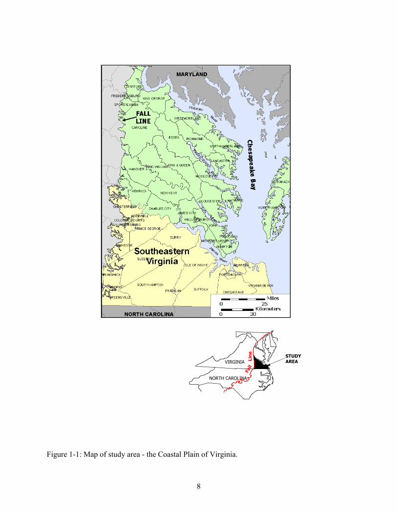
Figure 1-1: Map of study area - the Coastal Plain of Virginia.
8
NORTH CAROLINA
VIRGINIA
FallLine
STUDYAREA

Figure 1-2: Potentiometric surface of the Middle Potomac aquifer in 1998, developed from USGS water-level data. Hydraulic head values have units of meters relative to the sea-level datum. Red crosses indicate extensometer locations.
9

Figure 1-3: Rate of vertical land surface movement (mm/year), adapted from Holdahl and Morrison (1974).
10

II: ANALYTICAL APPROACH FOR AQUIFER-SYSTEM COMPACTION
Land subsidence due to the withdrawal of groundwater has a number of known causes,
but the mechanism considered here is compaction of the aquifer system. The process of aquifer-
system compaction is considered to be fairly well understood, although recent research has
focused on new aspects of the problem, such as deformation in three dimensions. Most simply,
the removal of groundwater from an aquifer or aquifer system causes a reduction in the fluid
pressure in the pores of the granular matrix. This loss of fluid pressure results in stress on the
aquifer matrix (skeleton), because the weight of the overlying materials supported by the
skeleton does not typically change significantly. The increasing stress on the aquifer skeleton
causes it to deform, particularly if the formation is unconsolidated or only partially consolidated.
The skeleton deforms or compacts in three dimensions, but deformation in the vertical direction
is the most noticeable and easiest to measure. This vertical compaction of the aquifer system is
usually expressed as subsidence of the land surface. The nature of the compaction and
subsidence in an aquifer system is controlled by a number of variables, including the patterns of
withdrawals and associated water-level declines, as well as the compressibility, permeability,
storage coefficient, and thickness of compacting units. While some recoverable compaction
occurs in coarse-grained aquifer units, most nonrecoverable compaction occurs as the result of
slow, irreversible consolidation of fine-grained confining units or aquitards. The understanding
of this process, known as the aquitard-drainage model, is the foundation of most research in
subsidence (Galloway and others, 1999).
Principle of Effective Stress and One-Dimensional Compaction
The development of the theoretical relationship between groundwater levels and
compaction of the aquifer system begins with the principle of effective stress originally proposed
by Terzaghi (1925, 1948) and represented in figure 2-1. In his theory of consolidation, Terzaghi
(1948) developed an expression to describe the vertical stress on a horizontal plane at any depth
below land surface in a system at equilibrium. His simple yet powerful relation is expressed as
PeT +=σσ (2-1)
where σT is the total stress due to the geostatic load [N/m2],
11

σe is the effective or intergranular stress [N/m2], and
P is the pore-water stress [N/m2].
Effective stress is defined by Lofgren (1969) as “the grain-to-grain stress which effectively
changes the void ratio and mechanical properties of a deposit.” Because the analysis of effective
stress is the most important consideration in studies of aquifer-system compaction and
subsidence, Terzaghi’s equation is simply rearranged, by Helm (1975), to solve for effective
stress:
PTe −=σσ (2-2)
This form of the equation explicitly reveals that the effective stress on the aquifer-system can be
increased by increasing the total stress (increasing the overburden) or by removing water and
decreasing the pore water stress (Helm, 1975). Of course, both of these phenomena may occur
together, and their effects are additive (Helm, 1975). This relation is outlined in greater detail by
Hanson (1989), who provides a means for calculating the components of the opposing stresses at
any depth z in a vertical column of unit area. The total stress is divided into three separate terms
(Hanson, 1989):
∫∫∫ −++=z
w
z
z w
z
wT gdzGngdzngdzSnw
w
00)1( ρρρσ (2-3)
Where zw is the depth below land surface to water table [m],
S is the degree of saturation above water table [dimensionless],
n is the average porosity [dimensionless],
ρw is the density of water [kg/m3],
Z is depth below land surface [m],
G is the specific gravity of solid grains in aquifer system [dimensionless].
The first term quantifies the weight of the water above the water table, the second term
represents the weight of the water below the water table, and the final term is the weight of the
sediments in the column. The pore-water pressure component of the effective stress, which
supplies an upward buoyant force in the system, can be expressed as (Hanson, 1989):
∫−=z
z ww
gdzP ρ (2-4)
12

This analysis demonstrates why stresses must be considered differently depending on whether
water is removed from a confined or unconfined aquifer. The removal of water from an
unconfined aquifer typically results in a change in the both the total stress (overburden) and the
pore water stress, while the removal of water from a confined aquifer usually results in a change
in the pore water stress only, for reasons explained below (Poland and others, 1975; Helm,
1975).
Stress or pressure, typically expressed in units of ML-1T-2, can also be expressed in terms
of equivalent hydraulic head (pressure head), with units of length L, by the following relation
(Sneed and Galloway, 2000):
gPhwρ
= (2-5)
This conventional expression of stress as equivalent hydraulic head is valid given the following
assumptions: constant gravity and a uniform incompressible (negligibly compressible) fluid
(Sneed and Galloway, 2000). Under these standard conditions, one foot of water is equivalent to
a pressure of 0.433 lb/in2. This convention allows a convenient comparison of the magnitudes of
various stresses for groundwater systems.
The rise and fall of the water table in an unconfined aquifer causes changes in
gravitational stress by removing or supplying fluid (thereby changing the total stress, σT) and by
increasing or decreasing the hydrostatic pressure in the aquifer (thereby changing the pore-water
stress, P). Within the unconfined aquifer, these two forces change with opposite signs. For
example, a water-table decline results in a decrease in the total stress in the unconfined aquifer,
which tends to decrease the effective stress; however, the same decline reduces the pore pressure
in the aquifer, leading to an increase in effective stress. For the unconfined aquifer, the net
change is an increase in effective stress (Lofgren, 1968). Specifically, the effective stress change
in an unconfined system can be calculated (Epstein, 1987) as change in weight per unit area:
)( bme hw γγσ −∆=∆=∆ (2-6)
Where ∆h is the change in water table height [m],
γm is the unsaturated unit weight of sediments above depth z,
γb is the buoyant unit weight of sediments above depth z.
13

Such an increase in effective stress in the unconfined system may cause some recoverable
compaction in the aquifer, and it may also induce a small amount of nonrecoverable compaction
in fine-grained interbeds within the unconfined system. However, compaction in unconfined
aquifers is usually of relatively small magnitude, because the net stress change is small for a
given water-table decline, and unconfined aquifers are usually relatively thin, leading to small
water-level declines. Of greater significance to compaction is the effect of rising and falling
water tables in an unconfined aquifer on the change in total stress on the aquifer system,
including confined aquifers below. This discussion of stresses is included here for completeness,
but the unconfined system is negligible, and it is disregarded in the analysis of aquifer system
stresses and the resulting compaction in the Virginia Coastal Plain. The stress changes in the
confined units are of much greater importance.
In a confined aquifer system, changes in effective stress almost always result from
changes in the pore water stress. Unless dewatering (drainage of the aquifer pores) occurs, the
lowering of head in a confined aquifer system does not significantly change the gravitational
stress, because the amount of water withdrawn per unit area is negligible. The associated change
in fluid pressure in the pores of the aquifer system is much more significant (Poland and others,
1972). Thus, the increase in effective stress in a confined aquifer system is approximately equal
to the decrease in the pore-water pressure (Poland and others, 1972; Helm, 1975). Furthermore,
Terzaghi’s equation for effective stress is developed under the assumption that sediment-volume
reduction through vertical compaction in an aquifer system is equal to the volume of water
expelled (Hanson, 1989). The nature of this relation depends on the distribution of aquifers and
confining units and interbeds in the aquifer system.
Lowering the hydraulic head in a confined aquifer results in a decrease in fluid pressure
in the pores of the aquifer, which is equivalent to an increase in effective stress. While the total
stress on the system does not change, stress is shifted from the pore water to the skeleton as pore
pressure is reduced. In incremental terms, this relation can be expressed as
Pe ∆−=∆σ (2-7)
The increase in effective stress results in compaction of the aquifer and a slight reduction
in porosity as the granular skeleton is compressed and rearranged. It should be noted that the
granular skeleton of the aquifer system is considered to be much more compressible than the
individual grains (Helm, 1975), and the compressibility of the grains is therefore neglected in
14

this analysis. Compaction that occurs in an aquifer responds immediately to a decrease in fluid
pressure, and it may be recovered quickly with a restoration of fluid pressure (Poland and others,
1972). Furthermore, this compaction is usually relatively small in magnitude, because the coarse,
angular grains cannot be placed in a much more compact arrangement.
The situation is much different in a fine-grained confining unit or aquitard adjacent to an
aquifer in which hydraulic head is lowered. A decrease in pore-water stress in the aquifer is
equal to an increase in effective stress at the aquifer-aquitard boundary (Hanson, 1989), but the
dissipation of this stress by the expulsion of pore water is not immediate. Pore fluid pressure can
only equilibrate in the confining unit as quickly as water can flow out (Lofgren, 1968). A fine-
grained confining unit typically has a low vertical hydraulic conductivity and a relatively high
specific storage. As a result, the vertical escape of water and the adjustment of pore pressures
from a clay unit is typically very slow compared to the response of an aquifer (Poland and others,
1972). Thus, the increase in stress, and the associated compaction, take effect only as the pore
pressure in the confining unit or aquitard slowly declines toward that in the aquifer (Poland and
others, 1972). Some of the compaction that occurs in a fine-grained unit is recoverable or
reversible, but a large part of it results from an irreversible rearrangement of clay grains
(Lofgren, 1968). This mechanism, along with the typically higher porosity of clays, explains why
most compaction in a system occurs primarily in the fine-grained interbeds and confining units.
This process is the basis of the theory of hydrodynamic consolidation developed by Terzaghi
(1925) and illustrated in figure 2-2.
Elastic and Inelastic Compressibility (Specific Storage)
An understanding of the relation between stress (head decline) and strain (compaction) is
an integral part of subsidence analysis, as suggested by the discussion above. In fact, analysis of
the compaction of a geologic unit relies on the stress-compaction relation, which is best
quantified by the specific storage (Ss) of that unit (Jacob, 1940, 1950; Cooper, 1966):
)( βαρ ngS ws += (2-8)
where ρw is the density of water [kg/m3],
g is the acceleration due to gravity [m/s2],
α is the compressibility of the aquifer matrix [m2/N],
n is the porosity [dimensionless],
15

β is the compressibility of water [m2/N].
Specific storage is the amount of water per unit volume of a saturated formation that is stored or
expelled from storage owing to compressibility of both the mineral skeleton and the pore water
per unit change in head (Fetter, 1994). Because the compressibility of water is assumed to be
negligible compared to the compressibility of the skeleton in most compacting systems, the
specific storage equation can be further simplified:
gS wsk αρ=* (2-9)
This equation gives th f e portion of specific storage derived from the expansion or compression o
the skeleton and is usually called S*sk to indicate that it is the skeletal component of specific
storage. The asterisk indicates that this is the overall specific storage of the aquifer system,
including both aquifers and confining units, following the convention of Sneed and Gallowa
(2000). As the equation demonstrates, the compressibility term is the important link in relating
stress to strain. The coefficient of compressibility (α) can be defined as the empirical relation
between the loss of void space and the increase in effective stress (Hanson, 1989). Because th
compressibility of water is not considered here, this coefficient of compressibility should
formally be known as α*k, or the skeletal component of compressibility. The coefficient o
compressibility can also be defined as the empirical relation between the loss of void space a
the increase in effective stress (Hanson, 1989)
eσα ∆−
∆−=*
y
e
f
nd
e
d ratio (e = volume of pore space/volume of solids).
(2-10)
Where e is the average voi
If the deformation of an aquifer or confining unit is considered to be entirely vertical, the
loss of
void space can be expressed is terms of thickness. Formally, the relation is given between
vertical strain and the change in the average void ratio (Helm, 1975):
eb ∆−=∆
eb +10
(2-11)
where ∆b is vertical compaction [m],
ss [m], b is the initial confining unit thickne
16

∆b/b0 is the mean vertical strain, and
ertical column.
The expression of the change in void space as the change in vertical thickness is
importa tly
terms
∆e is the average change in void ratio over the v
nt because the vertical change in thickness is the strain parameter most convenien
measured. It has been shown previously that the change in effective stress can be measured as
the change in pore pressure, expressed in terms of hydraulic head. As a result, two readily
measurable parameters are available with which to characterize the stress/strain relation. In
of specific storage, this relation can now be expressed as follows (Hanson, 1989):
bb∆ )/( 0
esk gS
σρ
∆=* (2-12)
In this discussion of the stress/strain (or water-level/compaction) relation, a distinction
has not r
y
arse-
s,
er system is less than any past maximum stress (drawdown) it
has exp
e
yet been made between the behavior of coarse-grained aquifer material and the behavio
of the fine-grained aquitard or confining unit material. As the earlier discussion indicated,
however, this distinction is vital for a full understanding of the behavior of the system. Earl
researchers in subsidence recognized that the compaction of an aquifer system could be
represented as the combined effect of the short-term, recoverable (elastic) response of co
grained aquifer material and the delayed, non-recoverable (inelastic) response of fine-grained
confining unit or aquitard material. This theoretical approach involves a number of assumption
and results in some significant limitations (which will be discussed later), but it has been the
basis of most subsidence research.
When the stress on an aquif
erienced, the system responds to water-level changes by compacting and expanding
almost instantaneously in a recoverable or elastic manner. On the other hand, when the stress
exceeds the past maximum level, the system experiences non-recoverable compaction that is
typically of greater magnitude. These two processes are usually represented by the recoverabl
and nonrecoverable components of skeletal specific storage, or Sske and Sskv (Sneed and
Galloway, 2000):
S >=
<==
(max)
(max)
****
*eekvskv
eekeskesk whengS
whengS
σσρασσρα
(2-13)
17
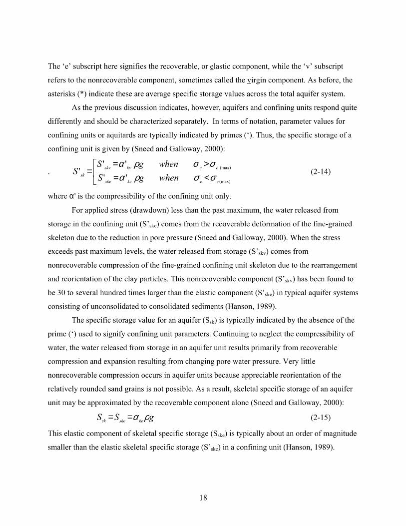
The ‘e’ subscript here signifies the recoverable, or elastic c
refers to the nonrecoverable component, sometimes called the v
omponent, while the ‘v’ subscript
irgin component. As before, the
asterisks (*) indicate these are average specific storage values across the total aquifer system.
confini
confining unit is given by (Sneed and Galloway, 2000):
As the previous discussion indicates, however, aquifers and confining units respond quite
differently and should be characterized separately. In terms of notation, parameter values for
ng units or aquitards are typically indicated by primes (‘). Thus, the specific storage of a
.
<=>=
=(max
(max)
''''
'eekeske
eekvskv
whengSwhengS
Sσσρασσρα
(2-14) )
sk
where α' is the compressibility of the confining unit only.
For applied stress (drawdown) less than the past maximum, the water released from
able deformation of the fine-grained
skeleto
nonrecoverable compression of the fine-grained confining unit skeleton due to the rearrangement
een found to
consisting of unconsolidated to consolidated sediments (Hanson, 1989).
ic
t the compressibility of
water, the water released from storage in an aquifer unit results primarily from recoverable
compression and expansion resulting from changing pore water pressure. Very little
an aquifer
unit may be approximated by the recoverable component alone (Sneed and Galloway, 2000):
storage in the confining unit (S’ske) comes from the recover
n due to the reduction in pore pressure (Sneed and Galloway, 2000). When the stress
exceeds past maximum levels, the water released from storage (S’skv) comes from
and reorientation of the clay particles. This nonrecoverable component (S’skv) has b
be 30 to several hundred times larger than the elastic component (S’ske) in typical aquifer systems
The specific storage value for an aquifer (Ssk) is typically ind ated by the absence of the
prime (‘) used to signify confining unit parameters. Continuing to neglec
nonrecoverable compression occurs in aquifer units because appreciable reorientation of the
relatively rounded sand grains is not possible. As a result, skeletal specific storage of
gSS keskesk ρα== (2-15)
This elastic component of skeletal specific storage (Sske) is typically about an order of magnitude
smaller than the elastic skeletal specific storage (S’ske) in a confining unit (Hanson, 1989).
18

As the above analysis demonstrates, the compaction of an aquifer system is driven primarily by
is
and strain is available from
laborat d
r
ne
at
should be noted that neither S’skv nor S’ske is actually constant. Rather, the actual values
of com
ide
ems
(Hanson, 1989).
the larger magnitude of compaction of fine-grained confining units and interbeds rather than
coarse-grained aquifer units. Aquifer units may contribute small but noticeable amounts of
recoverable compaction, but they typically contribute almost no permanent compaction. Not
surprisingly, then, the study of aquifer-system compaction and land subsidence is concerned
primarily with the strain behavior of confining units and interbeds under changes in stress. Th
subject is the most important component of the aquitard drainage.
Detailed knowledge of the empirical relation between stress
ory consolidimeter tests of samples taken from confining units (Helm, 1975). An idealize
diagram of the stress-strain behavior of a compacting clay (figure 2-3) provides a graphical
representation of this relation, which can also be applied to the behavior of a confining unit o
aquitard (Helm, 1975). As the confining unit is subjected to stress (drawdown) greater than any
experienced in the past, nonrecoverable strain (compaction) occurs along the solid curve from
point A to point B, resulting in a significant and permanent increase in strain represented as the
decrease in void space between those points (Helm, 1975). If the water level recovers, resulting
in a stress decrease, the strain decreases along the solid curve from point B to C in figure 2-3,
resulting in a small increase in void space, or expansion. From the stress level represented by
point C, stress less than that experienced previously results in recompaction along the dotted li
from C to B. This compaction, however, is reversible within the allowable range of stresses, and
the confining unit or aquitard may again expand along the curve from B to C. This hysteresis is
often observed both in the laboratory and in the field (Helm, 1975; Riley, 1969). Further
nonrecoverable compaction will occur only when the stress level again exceeds that found
point B.
It
pressibility and S’sk at a particular stress (water) level are given by the slope of the tangent
to the compaction curve at that point (Helm, 1975). In practice, the linear approximations
represented by the dashed lines from A to B and from C to B in figure 2-3 are used to prov
mean compaction and storage values over given ranges of stress because the actual values can
not usually be measured in the field. These linear estimates are considered to be reasonably
accurate under the ranges of stress and strain usually experienced in compacting aquifer syst
19

Delayed Drainage of Confining Units
The pore water stress component of Terzaghi’s equation, P, is divided by Helm (1975)
e equilibrium head in the pore water and U is the
transien
ater
e-
ss,
into two parts: P = Ps + U, where Ps is th
t pore-water stress in excess of the equilibrium. This approach provides a useful
understanding of the behavior of the system. As Helm (1975) points out, the excess pore w
stress P decays slowly to zero as water flows from an area of higher pressure within a fin
grained unit until the stress equilibrium is approached. The stress equilibrium is reached almost
instantaneously in an aquifer, while the process occurs much more slowly in a fine-grained
confining unit or aquitard, as explained above. The time τ required for a fine-grained unit to
reach equilibrium varies directly with specific storage and with the square of the unit thickne
and it varies inversely with the vertical hydraulic conductivity of the fine-grained unit (Riley,
1969). For a symmetrical, doubly-draining unit, this time constant is defined by Riley (1969):
( )'
2' '0b
KS=τ (2-16) 2
v
skv
These concepts, which collectively describe both the time-dependent nature of stress
(head change) throughout a fine-grained unit and the strain (compaction) response of the unit to
the stre ce
n of Assumptions
The development of the theory of hydrodynamic compaction and the aquitard drainage
ased on a number of assumptions that are either implied or stated
through
is of
ss, comprise the aquitard drainage model that has been the basis of most land subsiden
research.
Discussio
model as described here are b
out the discussion. The assumption of purely vertical strain merits special consideration
here. The definition of the storage coefficient in equation 2-8 (Jacob, 1940) is based on the
assumption that the volume reduction resulting from compaction of the aquifer skeleton occurs
entirely in the vertical direction. Consequently, this underlying assumption has been the bas
many of the conceptual and numerical models addressing the problem of aquifer-system
compaction, but it is known to be invalid (Burbey, 2001). In fact, it has been shown that the loss
of void space is the result of strain in three dimensions (Helm, 1974).
20

Horizontal displacement has been neglected partly because it has been thought to be
small, but theories of aquifer mechanics, three-dimensional simulations, and recent field data all
indicat
ts
f vertical strain are
conside
d.
e that horizontal strain may be significant, especially in conditions of radial flow to a
pumping center. While strain in three dimensions is not addressed in depth here, much current
research in the field of land subsidence is focused on this subject.
In practice, the equations governing strictly vertical compaction are more manageable, i
numerical computation is much simpler, and field measurements o
rably easier. For these reasons, this study and many others have continued to apply the
assumption of strictly vertical strain, but the limitations of this approach should be note
21

Figure 2-1: The principle of effective stress applied to land subsidence. Modified from Sneed and Galloway (2000).
22

Figure 2-2: Land subsidence due to the change in thickness in a multi-layer aquifer system resulting from a decline in hydraulic head in a confined aquifer.
23
Land surface
Land surface
Permanent subsidence due to nonrecoverablecompaction
Reversible subsidence due to recoverable compaction
Unconfined aquifer
Confined aquifer
Confining unit
Piezometer

Figure 2-3: Idealized stress-strain relationship in a fine-grained unit. Modified from Helm (1975). See text for full description of diagram.
24

III: HYDROGEOLOGIC SETTING Previous Work in the Coastal Plain of Virginia
Clark and Miller (1912) provided the first comprehensive report on the geology of the
Virginia Coastal Plain, while Sanford (1913) delivered an early analysis unifying the region’s
geology and groundwater resources. Cederstrom (1945, 1957) carried out a large amount of work
in the Virginia Coastal Plain and provided thorough descriptions of the hydrogeology of
southeastern Virginia (1945) and the York-James Peninsula (1957). In addition to describing and
correlating hydrogeologic units, Cederstrom’s works also supplied a large amount of useful
information on groundwater quality, usage patterns, and the history of groundwater development
in the Virginia Coastal Plain. A number of subsequent reports have described various aspects of
geology and hydrogeology in the Coastal Plain of Virginia, including stratigraphy, geochemistry,
and aquifer properties. Reports by Brown and Cosner (1974), Cosner (1975) and Hopkins and
others (1981), describing groundwater conditions in the Coastal Plain were of particular
relevance to the current work, as were reports on eastern Virginia water resources provided by
Richardson and others (1988), Kull and Laczniak (1987), and Laczniak and Meng (1988).
Meng and Harsh (1988) integrated the available data on geology and hydrogeology to
create the first complete hydrogeologic framework of the Coastal Plain in Virginia. Recently
available geophysical, palynological, and deep core data allowed Meng and Harsh (1988) to
refine and expand upon the conclusions of earlier authors. Their study, completed as part of the
Regional Aquifer System Analysis (RASA) program of the USGS, remains the definitive work
on Coastal Plain hydrogeology in Virginia and was immensely helpful in the completion of the
current research. Harsh and Laczniak (1990) expanded on the work of Meng and Harsh with a
detailed analysis of the Coastal Plain groundwater flow system in Virginia. Their work included
the development of a computer flow model for the Virginia Coastal Plain aquifer system using
the framework of Meng and Harsh (1988), and it significantly enhanced the current
understanding of the behavior of the system. A related modeling study by Hamilton and Larson
(1988) focused on the hydrogeology of the Virginia Coastal Plain south of the James River, an
area known as southeastern Virginia. Aside from the detailed hydrogeologic data and analysis it
provided for that area, the Hamilton and Larson (1988) report was important because it included
a slight revision to the Coastal Plain framework developed by Meng and Harsh, adding one
additional aquifer and confining unit to the aquifer system. The Virginia studies were ultimately
25
incorporated into a comprehensive groundwater modeling study of the entire Northern Atlantic
Coastal Plain, which was completed as part of the RASA program (Leahy and Martin, 1993).
The recent discovery of a bolide impact crater beneath the Chesapeake Bay area (Poag
and others, 1994; Poag, 1997) has led to further reconsideration and revision of the geologic and
hydrogeologic framework of the Virginia Coastal Plain (Powars and Bruce, 1999). The 56-mile-
wide crater (figure 3-1) was created approximately 35 million years ago by the impact of a large
comet or meteorite, which disrupted the pre-impact sediments and rocks in the region (Powars,
2000). The presence of the crater has also apparently affected the geologic structure of the region
and influenced the subsequent deposition and erosion of sediments in the surrounding area
(Powars, 2000). Thus, while the most significant effects of the impact can be found within the
boundary of the crater, the impact and the crater it created appear to have influenced the geologic
history of most of the Virginia Coastal Plain (Powars and Bruce, 1999). As a result, Powars and
Bruce (1999) and Powars (2000) have proposed revisions to the geology of the Virginia Coastal
Plain reflecting these influences.
The framework outlined by Meng and Harsh (1988), with the addition of refinements
reported by Hamilton and Larson (1988), has for years been the accepted interpretation of the
Coastal Plain aquifer system in Virginia, particularly outside the boundary of the impact crater.
While Powars and Bruce (1999) correctly point out that the crater discovery has “revealed the
inadequacy of the layer-cake, multi-aquifer model” of the Virginia Coastal Plain, their revisions
to the framework focus on the geology and hydrogeology within the crater boundary, which is
beyond the scope of this work. Outside the crater boundary, the ‘original’ framework is
somewhat intact, though recent publications have revealed a number of problems with long-
accepted interpretations. Powars and Bruce (1999) address revisions to the geologic framework
on the York-James peninsula of Virginia, and Powers (2000) addresses related revisions to the
geologic framework south of the James. Not surprisingly, these revisions suggest some
associated changes in the hydrogeologic framework, which currently does not reflect the known
effects of the impact crater. Many of these changes are now being included in a reassessment of
the hydrogeologic framework by the Virginia District of the USGS Water Resources Division
(McFarland, oral communication, 2001). The comprehensive numerical model originally
developed by Harsh and Laczniak (1990) has been repeatedly updated and refined by the USGS
in order to incorporate new hydrogeologic data, reflect improvements in model design, and
26

support the more sophisticated application of the model as a water resource management tool
(McFarland, 1998). Another revision to the model is currently being undertaken by the USGS
and the Virginia Department of Environmental Quality in order to address these issues. Among
the many changes, the current model revision will reflect the numerous influences of the impact
crater on the hydrogeologic framework and groundwater conditions of the Virginia Coastal Plain
(Erwin and others, 1999; McFarland, oral communication, 2001).
The geologic units and related hydrogeologic framework described by the above authors
has been adopted as the basis for this work. The geologic history and descriptions of geologic
and hydrogeologic units provided here are simply summaries of the information provided in
those reports; while some synthesis is attempted, no further interpretations are made here.
Instead, this discussion is intended as a concise overview of the hydrogeology of the Virginia
Coastal Plain as it is currently understood. Importantly, no published reports yet consider the
effects of the impact crater or other revisions to the hydrogeologic framework in Virginia, and
such a task is well beyond the scope of this work, though not insignificant to it. As a result, some
aspects of the revision currently underway are discussed in this report, based on numerous and
lengthy oral communications with USGS hydrologist Randy McFarland (2001).
One further clarification on this subject is necessary. Much of the recent work, published
and unpublished, on the geology and hydrogeology of the Virginia Coastal Plain concerns the
geologic influence of a structural zone associated with (and approximately parallel to) the James
River. The apparent influence of this zone on Virginia Coastal Plain geology is such that
interpretations of geologic and hydrogeologic units are significantly different on either side of
this boundary (Powars and Bruce, 1999). A detailed analysis of these differences is underway
and, again, beyond the scope of this work. Nevertheless, a very brief discussion of the James
River structural zone is undertaken here, and some mention is made of the effects of that zone on
hydrogeology north of the James River. For the most part, however, the descriptions of the
geologic and hydrogeologic units undertaken here concern the units as identified south of the
James River, within the explicit study area of this work. These units are outlined in the chart in
figure 3-2.
27

Topography, Geology, and Depositional History
The Virginia Coastal Plain is part of the Atlantic Coastal Plain province, which extends
from Cape Cod, Massachusetts to the Gulf of Mexico, as described generally by Heath (1983)
and others. While the various parts of the province share similar characteristics, only the Virginia
Coastal Plain is described here. The topography of the Virginia Coastal Plain was described
succinctly by Meng and Harsh (1988) as, “a series of broad, gently sloping, highly dissected
terraces bounded by seaward-facing, ocean-cut escarpments extending generally north-south
across the province.” Most of the Coastal Plain in Virginia is less than 100 ft in elevation, with
the highest elevations found along the Fall Line (Meng and Harsh, 1988).
Geologically, the Coastal Plain in Virginia can be most simply described as a
sedimentary wedge of unconsolidated gravels, sands, silts, and clays with variable amounts of
shells (Meng and Harsh, 1988). This sedimentary wedge (figure 3-3) thickens to the east, ranging
in thickness from almost zero at the Fall Line to over 6,000 ft beneath the Eastern Shore
Peninsula (Meng and Harsh, 1988). All units dip approximately to the southeast and strike
approximately parallel to the Fall Line, though, as Meng and Harsh (1988) point out, the dip of
each successive depositional unit decreases upward. As a result, the oldest and lowermost
deposits dip at 40 ft/mi along the basement surface, while the youngest surficial deposits dip less
than 3 ft/mi.
The unconsolidated sediments range in age from Early Cretaceous to Holocene (figure 3-
2) and indicate a complex history of deposition and erosion outlined by Meng and Harsh (1988)
as “a thick sequence of nonmarine deposits overlain by a much thinner sequence of marine
deposits.” The sedimentary deposits rest on a crystalline rock basement that is a combination of
massive igneous and highly deformed metamorphic rocks ranging in age from Precambrian to
Lower Paleozoic, along with some unmetamorphosed consolidated sediments and igneous
intrusives of Triassic age (Meng and Harsh, 1988).
Meng and Harsh (1988) divide the Coastal Plain sediments of the Virginia Coastal Plain
into five principal lithostratigraphic groups based on the mode of deposition. From oldest to
youngest, these groups are the Lower Cretaceous and lowermost part of the Upper Cretaceous
Potomac Formation; the uppermost Cretaceous deposits; the lower Tertiary Pamunkey Group;
the upper Tertiary Chesapeake Group; and undifferentiated Quaternary sediments (Meng and
Harsh, 1988) (figure 3-2).
28

The thick sedimentary sequences of the Early Cretaceous group resulted from the
deposition of continental and marginal marine sediments by rivers, which formed large subaerial
deltas on the broad underlying rock surface. The fluvial-deltaic nature of this deposition
produced interfingering sandy channel deposits and clayey inter-channel deposits. As a result,
these early Cretaceous sediments vary laterally and are known to thicken, thin, or pinch out over
relatively short distances (Hamilton and Larson, 1988). Even so, they make up approximately 70
percent of the thickness of the Coastal Plain sequence (Hamilton and Larson, 1988). The first
marine transgression early in the Late Cretaceous inundated the area with shallow seas and
extensive estuaries. After a long period of non-deposition as a result of a marine regression early
in the Late Cretaceous, a marine transgression deposited the clays, sandy clays and marls of the
uppermost Cretaceous group. The relatively thin but areally extensive sediments that form the
two Tertiary groups were deposited by what Meng and Harsh describe as interbasinal marine
seas. The Pamunkey Group of the lower Tertiary comprises glauconitic sands, silts and clays,
while the Chesapeake Group of the upper Tertiary is composed of shelly clays, silts, and sandy
clays. Because of the widespread and uniform nature of the transgressing seas, the Tertiary
deposits are relatively homogeneous and uniform throughout the Coastal Plain (Hamilton and
Larson, 1988), except where they have been disrupted by the Chesapeake Bay impact crater
(Powars and Bruce, 1999).
The impact crater itself was created in the late Eocene, when the coastline was west of
the present-day Fall Line (Poag and others, 1994). The comet or meteorite that struck the inner
continental shelf disrupted the entire Eocene to Cretaceous sedimentary sequence and penetrated
into the underlying crystalline basement rocks of Proterozoic to Paleozoic age. The impact
caused the ejection of a large amount of debris and generated a series of large tsunamis that
spread the debris over most of what is now the U.S. Atlantic continental shelf (Poag and others,
1994). The result of the impact was a complex crater 56 miles wide and about 1.3 miles deep,
underlain and surrounded by a zone of shocked, fractured and faulted crystalline basement rock
that extends to a depth of over six miles (Powars and Bruce, 1999). The crater was partially filled
almost immediately with collapsed and slumped material from the crater rim, as well as a chaotic
mix of sediments from the pre-impact sequence (Powars and Bruce, 1999). The sediments
deposited at the time of the impact are divided into two principal depositional units by Poag
(1997): the Chesapeake Bay impact crater megablock beds and the overlying Exmore tsunami-
29

breccia deposits. The megablock beds are found directly above the crystalline basement inside
the crater rim and are interpreted as consisting primarily of “Lower Cretaceous fluvial-deltaic
deposits that slumped into the crater during an early stage of crater filling and covered the floor
of the annular trough” (Powars and Bruce, 1999). These megablock beds range from 700 to
2,500 feet in thickness (Powars and Bruce, 1999). The tsunami-breccia deposits overlie either the
previously described megablock beds or the crystalline basement within the crater or the pre-
impact lower Cretaceous deposits outside the crater rim. The tsunami-breccia unit is described by
Powars and Bruce as having “a highly variable lithology,” consisting of a fining-upward
sequence of sand containing abundant material from all pre-impact sedimentary units, as well as
“trace amounts of shocked quartz”, “fragments of melt rock,” and scattered clasts of crystalline
basement,” containing deformation features (Poag and others, 1994; Powars and Bruce, 1999).
The thickness of the tsunami-breccia is highly variable, but estimated to reach a maximum of
over 2,000 feet inside the inner basin of the crater (Powars and Bruce, 1999).
Within the crater, post-impact upper Eocene sediments cap the Exmore tsunami-breccia,
but upper Oligocene sedimentary units are the earliest to be preserved without disruption across
the crater boundary (Powars and Bruce, 1999). Beginning with this upper Oligocene unit, the
crater is buried under hundreds of feet of post-impact sediments resulting from a series of marine
transgressions across the mid-Atlantic Coastal Plain in the late Tertiary (Powars and Bruce,
1999). While they are not disrupted by the crater boundary, sedimentary units deposited since the
impact tend to thicken into the crater, demonstrating the control on the depositional environment
by the structural depression associated with the crater (Powars and Bruce, 1999). However, this
structural influence becomes less apparent in later sediments, and is almost absent outside the
disruption boundary.
Across the Virginia Coastal Plain outside the crater, the Tertiary deposits are overlain by
Quaternary fluvial and marine deposits that are interpreted as reflecting Pleistocene sea-level
fluctuations. Cycles of erosion due to sea-level drops and deposition due to sea-level rises
produced drowned and infilled river valleys and extensive terraces (Hamilton and Larson, 1988).
Overlying the Pleistocene sediments, but included in the same group by Meng and Harsh, is a
thin layer of Holocene sediments deposited in lagoons, beaches and tidal flats during rising sea
levels since the Pleistocene (Hamilton and Larson, 1988). Within the crater boundary, the
Pliocene to Quaternary deposits are thought to be influenced by continued structural deformation
30

associated with the crater (Powars, 2000), but the influence of the crater on Quaternary
sediments is otherwise minimal.
A discussion of Coastal Plain geology and hydrogeology would be incomplete without
some consideration of the structural setting, which has played a significant role in controlling
deposition. The Coastal Plain as a whole is characterized as a regionally downwarped feature
controlled by crustal deformation, but local variations in this regional structure are significant.
The structural highs and lows associated with the Coastal Plain in Virginia are described by
Meng and Harsh (1988), but were previously recognized by a number of authors.
The feature most important to this study is the structural high known as the Norfolk Arch,
located near and approximately parallel to the present-day James River (figure 3-2). Its axis,
which dips to the southeast, divides the Salisbury embayment to the north and the Albemarle
embayment to the south (Meng and Harsh, 1988). The influence of the arch and these two basins
on the depositional history of the Coastal Plain is described in detail by Meng and Harsh (1988),
and later by Powars and Bruce (1999) and Powars (2000). The later authors provide more detail
on the structural complexity of this feature, describing a “James River structural zone”
coincident with the north flank of the Norfolk arch (Powars, 2000). Together with this structural
zone, the arch forms the northern boundary of the study area for the current work. In short, these
structural features are thought to be the controlling factors in the formation of two distinct basins.
The influence of this feature on the depositional environment appears to have become less
significant with time, as late Tertiary and subsequent deposits do not seem to be affected by the
arch and embayment structure (Meng and Harsh, 1988).
Hydrogeologic Framework
Descriptions and hydrogeologic data are given here for nine major confined aquifers,
nine associated confining units, and the uppermost water-table aquifer, following the framework
as developed by Meng and Harsh (1988), modified by Hamilton and Larson (1988), and outlined
by McFarland (1998). Hydrogeologic units are described in order from oldest to youngest, and
units characterized include those identified in the most recent modeling efforts (McFarland,
1998). While all units present in the Virginia Coastal Plain are described here for completeness,
it should be noted that not all of these units are found in southeastern Virginia, which is the area
most important to the current work.
31

The current framework (figure 3-4) does not yet include the modifications proposed by
Powars and Bruce (1999) and Powars (2000), reflecting the hydrogeologic effects of the
recently-discovered Chesapeake Bay impact crater. While these recent reports on the effects of
the crater have begun to answer some important and formerly unsolved questions about the
Coastal Plain aquifer system in Virginia, the analysis of the crater’s effects is not yet complete.
Powars (2000) argues convincingly for a revision of the current framework, pointing out the
problems with attempting to correlate the units of the current hydrogeologic framework with the
geologic units inside the crater’s disruption boundary. Nonetheless, such a revision has not yet
been completed. Furthermore, most of the Coastal Plain aquifer system outside the area of the
crater’s direct influence can still be described adequately, if not completely, by the framework as
it currently exists. Nonetheless, data from the recent studies have been incorporated into this
work, and comments concerning the influence of the crater on regional hydrogeology have also
been included where appropriate.
As is usually the case, the hydrogeologic units described by the above authors are defined
by lithologic and hydrologic properties rather than by their stratigraphic boundaries. Thus, a
hydrogeologic unit might be composed of several similar geologic formations, or a single
geologic formation with lithologic variations might be divided into an aquifer and a confining
unit. Analyses of water-level data were used to confirm and support these decisions (Meng and
Harsh, 1988). As Meng and Harsh (1988) point out, it is not uncommon for a hydrogeologic unit
to consist of combinations or divisions of geologic formations (1988). Nonetheless, the name of
a particular hydrogeologic unit, whether aquifer or confining unit, is based on the name of the
geologic formation or formations most closely associated with that unit. For example, the
Nanjemoy-Marlboro clay confining unit described below is made up of both the upper Paleocene
Marlboro clay and the lower Eocene Nanjemoy formation (Meng and Harsh, 1988). Further data
and justification for the differentiation of these hydrogeologic units can be found in the reports
that collectively define the Virginia Coastal Plain hydrogeologic framework (Meng and Harsh,
1988; Hamilton and Larson, 1998; Harsh and Laczniak, 1990). For the purposes of this report,
figure 3-2 provides an overview of the general correlations of the Virginia Coastal Plain aquifer
system units with the geologic units of the same area. The upper Eocene geologic units
associated with the Chesapeake Bay impact crater are not depicted in this figure.
32

The summary of hydrogeologic units given below includes a general overview of each
unit, including lithologic and stratigraphic information, inferred depositional environments,
inventories of known hydrogeologic properties, and information on water supply issues
associated with each of the units. In addition to the referenced publications, extensive oral
communication and written correspondence with the staff of the Virginia Division of the USGS
Water Resources Division were invaluable in the compilation of this information.
Lower Potomac Aquifer The Lower Potomac aquifer is the lowermost confined aquifer in the hydrogeologic
framework defined by Meng and Harsh (1988). It consists of “thick, interbedded sequences of
angular to subangular coarse sands, clayey sands and clays”, which range in age from early to
middle Early Cretaceous (Meng and Harsh, 1988). This wedge-shaped unit strikes approximately
north-south and dips eastward at approximately 40 ft/mi (5.7 m/km), extending across the entire
Coastal Plain of Virginia (figure 3-5). It thickens eastward from a thickness of almost zero at the
Fall Line to a maximum of over 3,000 ft near the Atlantic coast. Throughout its extent, the
Lower Potomac aquifer rests entirely and unconformably on the basement surface and is overlain
by the Lower Potomac confining unit.
The sands of the Lower Potomac aquifer are crossbedded and contain a high amount of
interstitial clays, as well as many clay lenses and beds. The sands themselves have commonly
been described as coarse and gray. More specifically, they are composed of medium to very
coarse subangular quartz, with abundant weathered potassium feldspar and some plagioclase
(Meng and Harsh, 1988). The “light to drab-colored” well-bedded clays are typically composed
of “mixed-layer illite/smectite,” according to lithostratigraphic descriptions, while the
“interstitial and laminated clays” are composed primarily of kaolinite (Reinhardt and others,
1980). Electric resistivity logs show patterns that are “blocky in profile, indicating massively
bedded sequences with relatively sharp lithologic contacts among sands, clayey sands and clays”
(Meng and Harsh, 1988).
An understanding of the depositional environment which formed this unit is helpful in
explaining what Meng and Harsh (1988) call “the lithologic heterogeneity and discontinuous
nature” of the Lower Potomac aquifer sediments. The sediments here are known to be poorly
sorted and contain a large amount of coarse material. This evidence, along with bedding
33

characteristics, has led several studies to suggest that these sediments represent the development
of a continental delta in a broad alluvial plain dominated by braided streams and occasionally
inundated by marine seas (Meng and Harsh, 1988). This mode of deposition explains why the
clay beds found within the unit and in the overlying Lower Potomac confining unit are “not
continuous or areally extensive,” but consist instead of a series of “interlensing clayey deposits”
(Hamilton and Larson, 1988).
The extremely variable and heterogeneous nature of the Cretaceous clays has become
increasingly apparent with recent work and has caused some geologists and hydrogeologists to
question the approach of defining distinct confining units in the Cretaceous sediments
(McFarland, oral communication, 2001). Instead, some have suggested that the Early-to-Middle
Cretaceous sediments of the Potomac Formation might better be represented as one large aquifer
with a number of discontinuous clay interbeds. While revisions to the hydrogeologic framework
currently in progress will likely take such an approach, all recent publications define several
distinct Cretaceous aquifers, and water-level and withdrawal data have been developed based on
that level of discretization. As a result, this report follows the approach taken in the recent
literature, but an attempt has been made to note the areas where the published work may not be
consistent with current understanding. While a detailed treatment of the potential revisions and
their development is beyond the scope of this work, an outline of the concepts behind them is
critical to a complete understanding of Coastal Plain hydrogeology and may be important in
understanding and analyzing land subsidence in this region.
The thickness of the Lower Potomac aquifer sediments, along with relatively high
hydraulic conductivity throughout, gives the aquifer large transmissivity values, generally
increasing in the down-dip direction. Aquifer tests at a variety of locations in the Coastal Plain
yielded mean transmissivity values of 12,000 to 19,000 ft2/d, or 1,115 to 1,765 m2/d, while
calibration of a groundwater flow model produced maximum transmissivity values of just over
12,000 ft2/d, or 1,115 m2/d (Harsh and Laczniak, 1990). Estimates and model calibrations
yielded average lateral hydraulic conductivity values from 25 to 42 ft/d, or 7.6 to 12.8 m/d
(Harsh and Laczniak, 1990). Aquifer storage coefficients, derived from the same aquifer tests,
range from 6.0 x 10⁻⁴ to 1.1 x 10⁻³. Storage coefficient values from flow models ranged from 8.0
x 10-6 to 2.5 x 10⁻⁴ (Hamilton and Larson, 1988).
34

As these high numbers indicate, the Lower Potomac aquifer is known to be capable of
producing large quantities of water. Yields from individual wells may exceed 1,500 gallons/min,
though the common range of yields is 100 to 800 gallons/min (Hamilton and Larson, 1990).
However, the depth of the aquifer below land surface, and the associated drilling and pumping
expenses, preclude use by all but the largest industrial applications, and only a handful of wells
penetrate this aquifer. Furthermore, increasingly high chloride concentrations in the down-dip
direction also restrict the use of groundwater from this aquifer (Meng and Harsh, 1988). Even so,
large industrial users make the Lower Potomac aquifer the third largest supplier of water in the
Coastal Plain, and withdrawals at several major pumping centers have caused tremendous
drawdowns in groundwater levels near those pumping centers and large associate cones of
depression. For example, water levels at the pumping center at Franklin, Virginia once rose over
20 ft above land surface (Cederstrom, 1945) but have fallen to 150 ft below sea level in recent
years (White and Powell, 1996).
Lower Potomac Confining Unit The Lower Potomac confining unit, which overlies the Lower Potomac aquifer, consists
of sequences of brown, gray, or dark-green carbonaceous clay, interbedded with thin, sandy clay
(Hamilton and Larson, 1988). While it is described as a confining unit, recent studies emphasize
the highly discontinuous and heterogeneous nature of the clays, pointing out that this supposed
unit demonstrates little lateral continuity. Revisions currently in progress will likely describe the
clays of this unit as another interbed in one large Potomac aquifer, as noted previously
(McFarland, oral communication, 2001).
The sediments of this unit are generally middle Early Cretaceous in age (Meng and
Harsh, 1988). Like the underlying Lower Potomac aquifer, this confining unit is thinnest along
the Fall Line and thickest toward the coast. It attains a maximum known thickness of 173 ft (52.7
m) in the northeastern part of the Coastal Plain (Meng and Harsh, 1988) and a maximum
thickness in the southeastern Virginia study area of approximately 80 ft (24.4 m) near the city of
Virginia Beach (Hamilton and Larson, 1988). The Lower Potomac confining unit rests atop the
Lower Potomac aquifer throughout the study area, except where the later crops out in stream
valleys near the Fall Line (Meng and Harsh, 1988). This confining unit is overlain by the Middle
Potomac aquifer.
35

The sediments of the Lower Potomac confining unit are referred to colloquially as “hard
and tough,” while lithologic studies describe the sequence as “a massive, clay-dominated interval
composed of thick sequences of finely laminated, carbonaceous clays interbedded with thin
sandy clay beds” (Meng and Harsh, 1988). More specifically, the thickly bedded clays of this
interval are identified as “mixed-layer illite/smectite” with a high percentage of expandable
clays, and the laminated carbonaceous clays found here are identified as “predominately
kaolinitic” (Reinhardt and others, 1980). Well logs indicate both “the sharp lithologic contacts
between the thickly-bedded confining clays and the overlying and underlying aquifer sands,” and
the “massively bedded nature” of these clays (Meng and Harsh, 1988). The lithology of this unit
distinguishes it from the underlying interbedded clays of the Lower Potomac aquifer, as the
aquifer clay units contain significantly more sands (Meng and Harsh, 1988).
Due to the depositional environment, the clay beds of this confining unit consist of a
series of “interlensing clayey deposits,” rather than a “continuous, areally extensive layer”
(Meng and Harsh, 1988). In this way, the unit is much like the interbedded clay units of the
underlying aquifer. Nonetheless, the “predominance of finer-grained clayey materials and their
associated bedding characteristics” in the Lower Potomac confining unit has caused several
studies to hypothesize a change in depositional environment from that of the Lower Potomac
aquifer. In general, the change is described as a progression from a “high-gradient to a lower-
gradient fluvial flood plain,” and the paleoenvironment is described as a “shallow, discontinuous
back-swamp basin” (Meng and Harsh, 1988).
While the clay deposits are not continuous, water-level observations indicate that the
interlensing causes the deposits to behave regionally as a single confining unit, and they are
represented as such in groundwater flow models (Harsh and Laczniak, 1990). Laboratory
analysis of the clays of this confining unit yielded a vertical hydraulic conductivity of 1.9 x 10⁻⁶
ft/d, or 5.8 x10⁻⁷ m/d (Harsh and Laczniak, 1990), though it should be noted that measurement
artifacts and field-scale heterogeneities generally cause laboratory measurements to
underestimate the actual values. One initial estimate gave a vertical hydraulic conductivity value
of 8.5 x 10⁻⁴ ft/d, or 2.6 x 10⁻⁴ m/d. (Harsh and Laczniak, 1990). Calibrations of groundwater
flow models yielded a range of 3.28 x 10⁻⁵ ft/d, or 1.00 x 10⁻⁵ m/d (Harsh and Laczniak, 1990) to
4.32 x 10⁻⁵ ft/d, or 1.32 x 10⁻⁵ m/d (Hamilton and Larson, 1988). Very little data are available for
calculating accurate specific storage values for this confining unit or others, and current models
36

do not consider the effects of water released from confining-unit storage (Harsh and Laczniak,
1990).
Middle Potomac Aquifer The Middle Potomac aquifer is the second lowest confined aquifer in the hydrogeologic
framework. Present throughout the Virginia Coastal Plain, it overlies the Lower Potomac
confining unit and underlies the Middle Potomac confining unit. It is confined throughout,
except for a narrow outcrop along the Fall Line (Harsh and Laczniak, 1990). It consists of
“interlensing medium sands, silts, and clays of differing thickness,” which are late Early
Cretaceous in age (Meng and Harsh, 1988). Like the Lower Potomac aquifer, this aquifer is
wedge-shaped and extends across almost the entire Coastal Plain, striking north-south and
dipping to the east at 15 to 25 ft/mi, or 2.8 to 4.7 m/km (Meng and Harsh, 1988) (figure 3-6).
From its western limit near the Fall Line, the Middle Potomac aquifer thickens to a maximum of
almost 1000 feet in the eastern part of the Coastal Plain (Meng and Harsh, 1988). Its similarity
with the Lower Potomac aquifer has caused some to suggest that it may be best defined as part of
that unit, though water levels indicate definite vertical gradients across the two units (McFarland,
oral communication, 2001).
The sediments of the Middle Potomac aquifer are described by early studies as a thick
sequence of interbedded silty clays and fine to medium sands (Meng and Harsh, 1988). A later
lithostratigraphic study more specifically describes this unit as a “sand-dominated interval
characterized by distinct fining-upwards sequences interbedded with laminated or massive clays”
(Reinhardt et al., 1980). The sands are described as being composed of “coarse to fine, angular to
subangular quartz, and some plagioclase,” and are also “commonly micaceous and contain
abundant heavy minerals” (Reinhardt et al., 1980). The “laminated and massive clays”
interbedded within this sequence are composed of “mixed kaolinite and highly expandable
illite/smectite” (Reinhardt et al., 1980). Well logs for this aquifer provide further information that
distinguishes this unit from the otherwise similar Lower Potomac aquifer. In particular,
resistivity logs show high-resistance values for the sands of the Middle Potomac aquifer,
reflecting both the clean sands of this unit and the relatively low concentrations of dissolved
solids in the water from this unit (Meng and Harsh, 1988). Furthermore, the resistivity log
patterns here are somewhat different from those of the Lower Potomac, showing “triangular and
37
saw-toothed” profiles rather than the blocky profiles of the Lower Potomac (Meng and Harsh,
1988). According to Meng and Harsh, the triangular profiles indicate “the fining-upwards
sequences characteristically associated with the aquifer sands,” while the saw-toothed profiles
indicate “the extensively interbedded sequences of sands, silts, and clays also characteristic of
these sediments.”
Of course, the lithologic character of the Middle Potomac aquifer sediments is closely
related to the environment of deposition, which consisted of “a low-gradient, subaerial, fluvial
flood plain dominated by meandering streams,” according to interpretations by Meng and Harsh
(1988) of earlier works by others. More specifically, these sedimentary deposits “are dominated
by channel sands, point bars, levees, flood plains, and backswamps, according to Meng and
Harsh (1988). A lithostratigraphic study (Reinhardt, 1980) notes the absence of glauconite in
these sediments and suggests that they are distinctly continental and represent a “more landward
assemblage,” than the sediments of the Lower Potomac aquifer (Meng and Harsh, 1988). The
sediments of the Middle Potomac aquifer, together with the underlying lower Potomac aquifer
sediments have been generally interpreted as representing the development of a continental delta
(Reinhardt and others, 1980).
As with the Lower Potomac aquifer, the large thickness and high hydraulic conductivity
throughout the Middle Potomac gives the aquifer relatively high transmissivity values. While
this aquifer unit thickens to the east, however, the transmissivity values generally decrease
seaward due to increasing amounts of silt and clay (Harsh and Laczniak, 1980). Aquifer tests
across the Virginia Coastal Plain produced average transmissivity values ranging from 2,000
ft2/d in the north-central Virginia Coastal Plain to a maximum of about 19,000 ft2/d or 1,765
m2/d in southeastern Virginia (Harsh and Laczniak, 1988). A measured transmissivity value of
56,800 ft2/d has been reported (Hamilton and Larson, 1988), but model calibrations support
maximum values of less than 19,000 ft2/d (Harsh and Laczniak, 1988; McFarland, 1998).
Estimates of average lateral hydraulic conductivity from model simulations ranged from
approximately 25 to 52 ft/d, or 7.6 to 15.8 m/d (Harsh and Laczniak, 1988). Storage coefficients
reported by Harsh and Laczniak from a number of sources range from 2.0 x 10⁻⁴ to 1.5 x 10⁻³,
though Hamilton and Larson (1988) reported storage coefficients ranging from 1.6 x 10⁻⁶ to 9.3 x
10-3, demonstrating a wide variation in the measurements.
38

The Middle Potomac aquifer provides the largest source of groundwater in the Virginia
Coastal Plain, and it is the primary source for large water users (Harsh and Laczniak, 1988).
Yields from wells penetrating this aquifer in southeastern Virginia have been reported to exceed
750 gal/min (Brown and Cosner, 1974), though common yields are reported to range from 20 to
160 gal/min (Hamilton and Larson, 1988). The aquifer is used by most municipal and industrial
water users in the western half of the Virginia Coastal Plain, but the depth of the aquifer makes
use prohibitively expensive for all but large industrial water users in the eastern half (Meng and
Harsh, 1988). As a result, the number of wells penetrating the aquifer tends to decrease toward
the coast. Withdrawals from the Middle Potomac aquifer began early in the 20th century and now
exceed 50 million gallons per day (Harsh and Laczniak, 1988). They have continued to increase
at a moderate rate (Harsh and Laczniak, 1988). These withdrawals have resulted in tremendous
declines in measured water levels, particularly over the decades following World War II. This
aquifer once produced flowing wells (Cederstrom, 1945), but groundwater levels have declined
to over 150 feet below sea level in recent years (White and Powell, 1996). As with the Lower
Potomac aquifer, high chloride concentrations restrict the use of water from the eastern part of
the Middle Potomac aquifer. Otherwise, the water quality is generally good, with relatively low
concentrations of dissolved solids (Meng and Harsh, 1988).
Middle Potomac Confining Unit The middle Potomac confining unit is defined by Meng and Harsh (1988) as “the major
clayey strata directly above the middle Potomac aquifer.” The confining unit overlies the middle
Potomac aquifer throughout its extent, except for a narrow outcrop of the aquifer along the
Potomac River in the northwestern part of the Virginia Coastal Plain (Harsh and Laczniak,
1990). It is overlain by the upper Potomac aquifer over most of its extent, except where it is
overlain by the Aquia in the western part of the Coastal Plain (Meng and Harsh, 1988). The
sediments of the confining unit are of late Early Cretaceous in age and comprise the middle part
of the Potomac formation (Harsh and Laczniak, 1990). Like the lower Potomac confining unit,
this unit is thinnest near the Fall Line and thickens toward the coast, obtaining a maximum
known thickness of just over 200 ft at a well on the Eastern Shore Peninsula (Meng and Harsh,
1988). The maximum known thickness in southeastern Virginia is 132 ft, measured in the city of
Chesapeake (Hamilton and Larson, 1988). Several sources describe the thickness of the middle
39

Potomac confining unit as highly variable, but it is commonly the thickest confining unit or
interbed found in the Potomac formation (Meng and Harsh, 1988). The average thickness used in
flow modeling is 40 ft (Harsh and Laczniak, 1990).
The sediments of the middle Potomac confining unit are characterized by “a thick
sequence of brightly-colored, highly variegated, plastic clays,” commonly used by drillers to
identify the unit (Meng and Harsh, 1988). These multicolored clays are also known as “mottled
clays,” and include red, purple, gray, brown, olive, and yellow units (Meng and Harsh, 1988).
The clays of the middle Potomac confining unit are similar in composition to those of the lower
Potomac confining unit described earlier; they contain primarily a mixture of kaolinite and
illite/smectite known to be highly expandable (Reinhardt and others, 1980). Another description
of this unit refers to the composition similarly as predominantly montmorillonitic red clays
(Harsh and Laczniak, 1988). Sources agree that the clays of this unit are usually massive and
thickly bedded, mottled, highly oxidized, and highly fractured, but they can also be finely
laminated in some places, in which case they are usually silty, sandy, micaceous, and
carbonaceous (Meng and Harsh, 1988; Harsh and Laczniak, 1990).
Like the lower Potomac confining unit, the middle Potomac confining unit is not
composed of a single, continuous layer, but can be characterized as “a series of interfingering
deposits” that together act as a single, regional confining unit (Meng and Harsh, 1988), albeit a
rather leaky one in places. These interfingering sedimentary units are the result of the
environment of deposition in which they formed. This environment is described concisely as
“broad, low-gradient fluvial-deltaic plains containing extensive flood plains and swampy
interfluves,” by Meng and Harsh (1988). Furthermore, the clay-dominated zones are specifically
described as “overbank deposition that was modified by weathering and diagenesis,” and are
considered to be “distinctly continental in origin” (Meng and Harsh, 1988).
While the middle Potomac confining unit is not a single, continuous layer, it is
represented as one in regional groundwater flow models (Harsh and Laczniak, 1990). Vertical
hydraulic conductivity of the unit was measured from laboratory analysis of a single core,
producing a value of 3.4 x 10⁻⁶ ft/d, or 1.0 x 10⁻⁶ (Harsh and Laczniak, 1990). Of course, a single
measurement like this would be expected to produce an artificially low value given the
discontinuous nature of this unit, and groundwater models confirm this expectation. Computer
simulations of this system produced what is probably a more realistic calibrated average value of
40

4.06 x 10⁻⁵ ft/d for the middle Potomac confining unit as a whole (Harsh and Laczniak, 1990).
An average specific storage value for this confining unit was estimate via model calibration as
1.0 x 10⁻⁶ ft-1, though it should be noted that groundwater simulations have not yet considered the
effects of the release of water from compressible deposits (Harsh and Laczniak, 1990).
Upper Potomac Aquifer The Brightseat-upper Potomac aquifer was originally defined by Meng and Harsh (1988)
as a continuous wedge of sandy sediments overlying the middle Potomac confining unit and
overlain by the upper Potomac confining unit (figure 3-7). The wedge-shaped aquifer of Late
Cretaceous age defined by Meng and Harsh thickened from its western edge roughly 20 to 30
miles east of the Fall Line to a maximum of over 400 feet in eastern Virginia, and it was
interpreted as representing the effects of the “first major marine transgression” across the
underlying continental delta complex (1988). Over a decade of further study since the work of
Meng and Harsh has revealed the geology and the associated hydrogeology of this interval to be
significantly more complex than what they described. Much of the complexity in the
interpretation of this interval apparently results from the transitional nature of the depositional
environment, which has been further complicated by the influence of the Norfolk arch and James
River structural zone, as well as the disruption attributed to the impact crater. Evidence for this
increased complexity is documented by Powars and Bruce (1999) and Powars (2000) and
suggests that the Brightseat-upper Potomac aquifer may be further subdivided in the future to
reflect spatial variations in the depositional environment and resultant hydrogeologic properties
(McFarland, oral communication, 2001). Consequently, some of the increased complexity
described by various authors is outlined here, particularly as it pertains to the hydrogeology of
southeastern Virginia.
In Virginia, no sediments of Late Cretaceous age have been found west of the
Chesapeake Bay and north of the James River (Powars and Bruce, 1999), so the upper Potomac
aquifer is no longer thought to exist in that area (McFarland, oral communication, 2001). Instead,
these sediments are known to be either Early Cretaceous or Paleocene in age (Powars and Bruce,
1999). Of course, the age of a sedimentary interval should not necessarily determine its
hydrogeologic delineation, but in this case the age relation is thought to be somewhat indicative
of hydrologic continuity, and these sediments are therefore classified as belonging either to the
41

Middle Potomac aquifer of continental origin or the Aquia aquifer of marine origin (McFarland,
oral communication, 2001). In any case, this issue is not particularly relevant to the
hydrogeology of southeastern Virginia. Similarly, the Brightseat Formation of Early Paleocene
age is no longer thought to exist in Virginia, so the Brightseat is no longer thought to be a part of
the upper Potomac aquifer or confining unit (Hamilton and Larson, 1988).
South of the James River, the sediments originally described as the upper Potomac
aquifer are of Late Cretaceous age and predominantly marine in origin, and the descriptions of
Meng and Harsh (1988) may be more or less accurate, if not complete. A complete
characterization of the increased complexity of this interval is again beyond the scope of this
work, but some discussion is included here because the increased detail provides a somewhat
better representation of spatial variability in hydrologic properties and behavior. The Upper
Cretaceous deposits south of the James were subdivided by Powars (1992, 2000) into three
lithologic units. He described (1) upper Cenomanian marine and deltaic deposits overlain by (2)
a loose glauconitic sand unit and (3) “oxidized red-bed fluvial-deltaic deposits that include
multiple paleosols” (Powars, 2000). The vertical relations between these units can be evaluated
from figure 3-3 and the chart in figure 3-2. Hydrogeologically, the upper Cenomanian beds
correspond with the upper Potomac aquifer described by Meng and Harsh (1988); the glauconitic
sand unit corresponds with the Virginia Beach aquifer described by Hamilton and Larson (1988);
and the red beds correspond roughly with either the upper Potomac confining unit of Meng and
Harsh (1988) or the Virginia Beach confining unit of Hamilton and Larson (1988). For
clarification, it should be noted that Hamilton and Larson recognized an eastward part of the
upper Potomac confining unit of Meng and Harsh as the separate Virginia Beach aquifer,
resulting in the arrangement depicted in figure 3-2. The Virginia Beach aquifer is described
separately on following pages.
As described by Meng and Harsh (1988) deposition of the upper Potomac aquifer
“occurred in everwidening estuaries and intertidal basins,” as the seas gradually and
progressively inundated the area (Meng and Harsh, 1988). Specific environments of deposition
postulated by other authors include a littoral, possibly tidal flat environment with a protected
shoreline, or a “marginal marine outer-delta environment with a vegetated, swampy shoreline”
(Meng and Harsh, 1988). Because of the change in depositional environment, revisions in
progress will likely distinguish the sediments of this aquifer with a name distinct from the other
42

Potomac aquifers, which belong to the Potomac formation of continental origin (McFarland, oral
communication, 2001).
The sandy units of the upper Potomac aquifer, as described from driller’s logs by Meng
and Harsh (1988), are “characteristically white, micaceous, very fine to medium quartz, and
commonly contain carbonaceous material.” The interbedded clays are described by drillers as
dark, silty, and highly micaceous, commonly containing carbonaceous material. Available
lithologic reports of core samples indicate that the upper Potomac aquifer consists of very fine to
medium, “yellow to greenish-gray” micaceous quartz sands that are “poor to well sorted,” and
“subrounded to subangular,” commonly containing wood fragments and “interstitial clays (Meng
and Harsh, 1988). Lithologic descriptions of interbedded silty-clay intervals describe them as
“yellow green to dark greenish gray, glauconitic, calcareous, micaceous, plastic,” and locally
sandy, commonly containing shell fragments (Meng and Harsh, 1988). Drillers commonly note
that these sediments are easily penetrated, according to Meng and Harsh. Geophysical logs
through the Upper Potomac aquifer show patterns similar to those found in the middle Potomac
aquifer, but they are “more massive and rounded in profile,” indicating more massively bedded
sands and thinner interbedded clays (Meng and Harsh, 1988). As in the middle Potomac aquifer,
the interlensing nature of the sands and clays and the difficulty in correlating the individual
layers cause authors to qualify given elevation and thickness measurements as approximate.
Nonetheless, the layers of the upper Potomac aquifer are described as easier to correlate spatially
than those of underlying units, probably due to changes in the depositional environment from
generally continental to marine (Meng and Harsh, 1988).
For the purposes of this study and the several groundwater modeling studies of the area,
the upper Potomac aquifer can be thought of as overlying the middle Potomac confining unit, but
it is not always present. The overlying unit varies spatially across the Coastal Plain of
southeastern Virginia. It is usually the Paleocene Aquia aquifer, but the overlying unit may also
be the Peedee aquifer or the Virginia Beach aquifer, depending on location. Collectively, the
predominantly marine sediments of the unit referred to as the upper Potomac aquifer by Harsh
and Laczniak reach a maximum thickness of approximately 425 ft in the northeastern part of the
Coastal Plain of Virginia (1990).
The upper Potomac aquifer is characterized hydrogeologically by high transmissivity
throughout most of its extent, though values decrease somewhat toward the coast. The decrease
43
in transmissivity was originally attributed to a facies change from sands to silts and clays, but it
may also be due to the effects of the impact crater boundary. Regardless of the cause, maximum
transmissivities can be found in southeastern Virginia, where values from aquifer tests range
from 1,500 to 13,000 ft2/d (Harsh and Laczniak, 1990). In other areas of Virginia, reported
values range from a minimum of about 150 ft2/d in the north-central Coastal Plain to 2,000 ft2/d
near the York River at West Point (Harsh and Laczniak, 1990). Flow-model calibrations
produced a transmissivity range of 330 to over 4,000 ft2/d (Harsh and Laczniak, 1990), while
revised model values approach 9,000 ft2/d in some locations (McFarland, 1998). The only
available value for the storage coefficient of this aquifer is provided by Harsh and Laczniak
(1990) in their modeling study of the Virginia Coastal Plain. Their reported mean value of
5 x 10⁻⁴ is calculated from several earlier aquifer tests. The same source estimates the average
lateral hydraulic conductivity of the upper Potomac aquifer to be approximately 25 ft/d.
The upper Potomac aquifer is the principal source of water for municipal, industrial, and
agricultural use in the eastern part of the Virginia Coastal Plain (Harsh and Laczniak, 1990).
Wells completed in the aquifer are reported to yield from 25 to 350 gal/min, according to several
sources, and numerous wells tap the aquifer (Harsh and Laczniak, 1990). With total reported
withdrawals from the upper Potomac aquifer in Virginia currently approaching 20 million
gallons per day, the aquifer ranks second behind only the middle Potomac as a source of water
for the Coastal Plain. As a result of this continued development, water levels in the upper
Potomac aquifer have declined from historic highs of over 20 ft above sea level to current lows
of 20 to 30 ft below sea level (Harsh and Laczniak, 1990). Continued withdrawals are expected
to lead to further declines in water levels.
Upper Potomac Confining Unit As with the upper Potomac aquifer, the Brightseat-upper Potomac confining unit is no
longer thought to include the Brightseat Formation (Hamilton and Larson, 1988; McFarland, oral
communication, 2001). The Brightseat aquifer and confining units, described by Meng and
Harsh (1988), were once thought to occur across the northeast quarter of the Virginia Coastal
Plain. Throughout their extent, they were described as overlying the upper Potomac aquifer and
confining unit, but these sediments are now thought to belong to the Aquia aquifer, or perhaps
the underlying upper Potomac. Furthermore, the upper Potomac confining unit described by
44

Meng and Harsh (1988) as extending across the Virginia Coastal Plain is now thought include
sediments of Early Cretaceous age north of the James River.
In other words, the proper “upper Potomac confining unit of Late Cretaceous age” only
exists south of the James River, while sediments of at a similar depth interval belong to the
Middle Potomac confining unit of Early Cretaceous age” north of the James. Regardless of
origin or name, these sediments together form the hydrogeologic model unit referred to by Harsh
and Laczniak (1990) as the Brightseat-upper Potomac confining unit, which consists of
sediments of possibly late Early Cretaceous to early Paleocene age directly underlying the
Paleocene sediments of the Aquia aquifer across the Coastal Plain of Virginia. Perhaps the
revisions currently underway will sort out this confusion. For now, this interval will be
collectively described as presented by Meng and Harsh (1988) and Hamilton and Larson (1988).
The upper Potomac confining unit varies in thickness throughout the Virginia Coastal
Plain, but it attains its maximum known thickness of 192 ft in southeastern Virginia (Hamilton
and Larson, 1988). The estimated average thickness of this unit used in groundwater models is
35 ft (Harsh and Laczniak, 1990). In general, this unit thickens and dips to the east. As described
by Hamilton and Larson, this clay unit continues across almost the entire Coastal Plain in
Virginia, giving the rather large combined areal extent (1988).
The sediments of the upper Potomac confining unit are collectively described as “dark-
green to black, highly micaceous silty clay with oxidized red to yellow thin clay” (Harsh and
Laczniak, 1990). Other descriptions of core note that this clay unit is also calcareous, slightly
glauconitic, and sandy (Meng and Harsh, 1988). More specifically, the clays consist of “highly
expandable silty-clay to clayey-silt mixed-layer illite and montmorillonite, and minor amounts of
kaolinite” (Meng and Harsh, 1988).
As with the lower and middle Potomac confining units, the clays of this confining unit
form a series of interlayered deposits rather than a single, continuous layer (Meng and Harsh,
1988). However, these layers and lenses of clay are more extensive than those found in the lower
confining units, so they can generally be more easily correlated between wells (Meng and Harsh,
1988). The deposition of these clays is interpreted as the result of the “first major marine
transgression in the sedimentary section,” and it probably occurred in a “broad, low-lying outer
delta” environment (Meng and Harsh, 1988). It now appears that this description may be most
45

accurate for the part of the unit found south of the James River, which may be correlated with the
upper Cenomanian beds described more recently by Powars (2000).
Laboratory analyses of core from this confining unit in Maryland yielded a vertical
hydraulic conductivity value of 8.64 x 10⁻⁴ ft/d, as well as a specific storage value of 7.4 x 10⁻⁵ ft-
1 (Harsh and Laczniak, 1990). The average vertical hydraulic conductivity value for this unit
obtained from calibration of model simulations was about an order of magnitude lower, at 4.41 x
10-5 ft/d, but the specific storage value from the calibrated model is similar to the value from
field measurements, at 1.0 x 10⁻⁶ ft-1 (Harsh and Laczniak, 1990).
Virginia Beach Aquifer Composed of unnamed Upper Cretaceous sediments, the Virginia Beach aquifer was first
recognized and named by Hamilton and Larson (1988). This aquifer unit is present only south of
the James River in Virginia and extends southward into northeastern North Carolina, where it is
equivalent to the Black Creek Formation (Hamilton and Larson, 1988) (figure 3-8). The Virginia
Beach aquifer pinches out to the west approximately 30 miles east of the Fall Line. It’s northern
edge, apparently controlled by the southern flank of the Norfolk arch, follows a line extending
from Virginia Beach southwestward to Suffolk, then just south of Franklin (Hamilton and
Larson, 1988). As a result, it is uncertain whether this unit is present at the location of the
subsidence wells at Franklin and Suffolk. In Virginia, the Virginia Beach aquifer dips to the east
and reaches a maximum thickness of approximately 110 feet at the city of Chesapeake (Hamilton
and Larson, 1988). Throughout its extent in Virginia, this aquifer and its confining unit are
overlain by the upper Paleocene Aquia aquifer. In northeastern North Carolina, the overlying
unit is the Peedee Aquifer.
The fine-grained to medium-grained glauconitic sands of the Virginia Beach aquifer are
interbedded with “thin clay layers and indurated zones,” and commonly contain shell material
(Hamilton and Larson, 1988). The sediments of the Virginia Beach aquifer described by
Hamilton and Larson (1988) correlate approximately with the Upper Cretaceous glauconitic sand
unit more recently described by Powars (2000). Powars describes the glauconitic sand unit as
loose, well-sorted, fine to very coarse glauconitic marine sand with very little clay or silt (2000),
which indicates that this glauconitic sand may be only part of the aquifer described by Hamilton
and Larson (1988).
46

Very little published data are available regarding the hydrogeologic properties of the
Virginia Beach aquifer. However, the Virginia Beach aquifer is part of a horizon that was
previously thought to be part of the upper Potomac, which is also composed of marine sands.
Consequently, the hydrologic properties outlined for the upper Potomac aquifer are probably
representative of the Virginia Beach aquifer.
The Virginia Beach aquifer is described by Hamilton and Larson as capable of producing
“moderate to abundant quantities of generally good quality” for domestic and industrial uses
(1988), though only from its up-dip area. In the thickest eastern parts of the aquifer, the water is
too brackish to be used as a water supply (Barry Smith, USGS, verbal communication, 2001).
Virginia Beach Confining Unit Little data are available regarding the character of the Virginia Beach confining unit,
which is described by Hamilton and Larson as a series of clay, silty clay and sandy clay beds
overlying the Virginia Beach aquifer throughout its extent (1988). According to their description,
this unit ranges in thickness from less than 10 feet along its updip edge to almost 30 feet near the
city of Virginia Beach (Hamilton and Larson, 1988). It now appears that this unit is likely part of
a geologic unit defined by Powars (2000). He identifies Upper Cretaceous red beds overlying the
glauconitic sand unit in southeastern Virginia (Powars, 2000). These red beds are described as
having a heterogeneous lithology of interbedded oxidized clay, silty fine sand and coarse sand
(Powars, 2000). Powars also describes fining-upward sequences that include clayey paleosols
(2000). These red beds and the underlying glauconitic sands form the Virginia Beach confining
unit and aquifer; this relation can be seen in Figure 3-2. The red beds are described as having a
“fluvial to upper-delta-plain depositional environment” because of their extensive development
(Powars, 2000).
The Virginia Beach confining unit includes sediments that were formerly defined as part
of the upper Potomac confining unit. As a result, the hydrogeologic characteristics of this unit
are likely very similar to those of the upper Potomac, but very little specific data are available on
the characteristics of the Virginia Beach confining unit. In general, the extent of the Virginia
Beach aquifer and confining unit are not particularly well defined. As Meng and Harsh point out,
it is relatively easy to distinguish the Cretaceous sediments of marine origin from the underlying
fluvial-deltaic sediments, using geophysical logs and available lithologic data (1988). On the
47

other hand, it appears to be much more difficult to distinguish the marine sediments from each
other. This has resulted in some misunderstanding of the relation between the upper Potomac and
Virginia Beach aquifers and confining units. Figure 3-3 and the chart in figure 3-2 outline the
current understanding of the system.
Peedee Aquifer The Peedee aquifer and overlying Peedee confining unit are present only in the
northeastern corner of North Carolina and are not found in Virginia (figure 3-9). These units are
Late Cretaceous in age and stratigraphically overlie the Virginia Beach aquifer and confining
unit throughout their extent. In thickness and hydrogeologic properties, these units are very
similar to the Virginia Beach units (Hamilton and Larson, 1988). They are mentioned here only
to provide completeness to the correlation of hydrogeologic units presented in Figure 3-2. More
detailed information is provided by Hamilton and Larson (1988).
Aquia Aquifer The Aquia aquifer is described by Meng and Harsh as the “predominantly sandy facies of
the Aquia Formation” of late Paleocene age (1988). It extends across most of the Coastal Plain of
Virginia and correlates with similar units in Maryland and North Carolina. The Aquia aquifer
overlies either the upper or middle Potomac confining unit and is overlain by the Nanjemoy-
Marlboro confining unit throughout its extent (Meng and Harsh, 1988). The Aquia aquifer attains
a maximum thickness of almost 150 feet; values range from about 40 to 70 feet throughout much
of its extent (Meng and Harsh, 1988), though lower values are reported for most locations in
southeastern Virginia (Powars, 2000), (figure 3-10). It extends to a thin edge just east of the Fall
Line, and it crops out in many stream valleys in the western part of the study area. Like most of
the other units of the Virginia Coastal Plain, the Aquia aquifer dips to the east. Unlike many of
the other Coastal Plain aquifers, however, the Aquia aquifer is described as thinning to the east
as the result of a facies change in the late Paleocene sediments (Meng and Harsh, 1988). It is
now known that the Aquia aquifer is also truncated to the east by the boundary of the
Chesapeake Bay impact crater (Powars, 2000). Within the crater boundary, sediments once
thought to be part of the Aquia aquifer are now known to be part of the Exmore tsunami-breccia
deposits (McFarland, USGS, verbal communication, 2001).
48

The Aquia aquifer is described as a “continuous, elongate-lenticular sand body” (Meng
and Harsh, 1988). It is a “massively bedded unit composed of very fine to medium glauconite
and quartz sands” with minor amounts of shells and clay (Meng and Harsh, 1988). The sands are
described in more detail by various authors as “greensands and greensand marls,” and “very
well-sorted, medium to dark green, massive, fine to medium glauconitic sand (Meng and Harsh,
1988). Most authors recognize sparse shelly intervals, carbonate cemented intervals, some thin
clay intervals, and a basal section containing sand, pebbles, and fish bones and teeth (Meng and
Harsh, 1988). Mica, pyrite, and lignitic material are also reported (Powars, 2000). The sediments
of the Aquia aquifer are often described colloquially as running or caving sands due to their soft
nature (Meng and Harsh, 1988). Unlike many of the underlying units, the Aquia aquifer can be
easily correlated across large distances due to distinctive geophysical log signatures as well as
very distinctive clay units which mark the top and bottom of the Aquifer sands on drillers’ logs
(Meng and Harsh, 1988). Most sources suggest that the depth to the top of the aquifer can be
predicted with confidence between control wells due to its consistency (Meng and Harsh, 1988;
McFarland, verbal communication, 2001).
The consistent lithology of the Aquia aquifer is due to its relatively consistent
depositional environment. According to the summary provided by Meng and Harsh, various
authors suggest that the unit was deposited “in a shallow, inner shelf marine basin, below wave
base, with slight fluctuation of water depths” from about 100 to 300 ft (1988). Similarly,
Hamilton and Larson describe the environment of deposition as “shallow marine waters” (1988).
The transmissivity of the Aquia aquifer has been measured from single-well and specific
capacity tests, and values are reported to range from 125 to 1000 ft2/d. Of course, values vary
with thickness, though an eastward facies change was also invoked to explain lower
transmissivities in that direction (Harsh and Laczniak, 1988). These variations are now thought
to be almost certainly the effects of the Chesapeake Bay impact crater. No data on the storage
coefficient are available for the Aquia aquifer in Virginia, but a range of 1.0 x 10⁻⁴ to 4.0 x 10⁻⁴ is
reported for the Aquia aquifer in Maryland (Harsh and Laczniak, 1990). Estimated and modeled
hydraulic conductivity values range from about 25 to 40 ft/d (Harsh and Laczniak, 1990).
The Aquia aquifer is a consistent and accessible source of water for a variety of small-
volume users. Numerous wells penetrate the aquifer across the Coastal Plain and within the study
area, though use of water from the Aquia is more common north of the James River, where the
49

aquifer is thicker and more sandy (Meng and Harsh, 1988). Wells in the Aquia are reported by
various authors to yield between 20 and 110 gallons per minute (Harsh and Laczniak, 1990),
though they are reported to exceed 550 gal/min (Kull and Laczniak, 1987). The Aquia aquifer
provides a water source for light industrial, small municipal and industrial users. Withdrawals
total a few million gallons per day for the Coastal Plain, just a few percent of groundwater
withdrawals from the Virginia Coastal Plain (Kull and Laczniak, 1987). Small but consistent
increases in withdrawals have been observed in recent decades.
Nanjemoy-Marlboro Confining Unit The Nanjemoy-Marlboro confining unit is composed of the clay deposits of two distinct
formations that together overlie the Aquia aquifer throughout its extent, except where the aquifer
crops out along its western edge. The Marlboro Clay of late Paleocene age directly overlies the
Aquia and is itself overlain by the Nanjemoy Formation of early Eocene age (Meng and Harsh,
1988). Together, these formations make up a generally wedge-shaped unit that thickens from
near zero along its western edge near the Fall Line to over 150 ft on the northern part of the
Eastern Shore Peninsula (Meng and Harsh, 1988). Its maximum thickness in southeastern
Virginia is 62 feet (Hamilton and Larson, 1988). The Nanjemoy-Marlboro confining unit is
described as very continuous, and its top elevation can usually be predicted with some
confidence between control wells (McFarland, oral communication, 2001). Furthermore, the
sediments of this unit are easily recognized on both resistivity and drillers’ logs because of their
characteristic thick clay pattern and distinctive colors; the contacts with the overlying and
underlying sandy aquifers are also distinctive and easily recognized (Meng and Harsh, 1988).
While the confining unit as a whole is described as easy to identify, the two units that
compose it are sometimes difficult to distinguish from each other, and there appears to be some
uncertainty regarding their areal extents. Meng and Harsh (1988) describe the Marlboro Clay as
pinching out against the northern flank of the Norfolk arch, but Powars (2000) finds this unit in
analysis of several core holes in southeastern Virginia. On its eastern edge, this unit is truncated
by the Chesapeake Bay impact crater and its infilled sediments.
The Marlboro Clay is composed of a distinctive red to gray mottled clay composed
primarily of kaolinite and illite (Meng and Harsh, 1988). It is described as massively bedded and
extensively burrowed, with irregular lenses of fine silt (Reinhardt and others, 1980). Drillers
50
often refer to it as “slick or sticky” and “pink, gray or white (Meng and Harsh, 1988). It ranges in
thickness from about 2 to 20 ft across the Coastal Plain (Meng and Harsh, 1988). The Nanjemoy
Formation is composed of a “variably clayey and shelly, micaceous greensand,” which is dark-
green to brown-green and massively bedded (Meng and Harsh, 1988). Extensive burrows give
the unit what is described as a mottled appearance (Meng and Harsh, 1988). The clay content is
mostly illite and ranges from 15 to 80 percent (Meng and Harsh, 1988). Drillers commonly note
the presence of shells and black sands (Meng and Harsh, 1988).
Distinct environments of deposition for the upper Paleocene Marlboro clay and the lower
Eocene Nanjemoy clay have been inferred from intensive analysis of core (Reinhardt et al.,
1980). The Marlboro clay is thought to have formed in a brackish, low-energy basin such as an
estuary or lagoon (Meng and Harsh, 1988). The Nanjemoy, on the other hand, was deposited in
an environment of somewhat higher energy, such as a protected inner middle marine shelf (Meng
and Harsh, 1988).
The average vertical hydraulic conductivity value for this unit from calibration of model
simulations was 5.36 x 10⁻⁵ ft/d. Vertical hydraulic conductivity values as determined from
laboratory analysis of core range from 2.0 x 10⁻⁵ to 2.2 x 10⁻⁶ (Harsh and Laczniak, 1990). This
confining unit is known to be much more areally extensive than some of the underlying units
already described, so laboratory analyses would be more likely to produce somewhat better
values for the behavior of the unit as a whole. Model calibrations used an estimated value of 1 x
10-6 ft-1 for the specific storage of this confining unit, but no other storage data are available.
Chickahominy-Piney Point Aquifer Definition of the Chickahominy-Piney Point aquifer (figure 3-11) is not possible without
some consideration of the role of the bolide impact and the crater it formed. The aquifer, as
described by Meng and Harsh, was thought to be composed of the sandy sediments of the middle
Eocene Piney Point Formation and the overlying Chickahominy Formation (1988). Meng and
Harsh recognized changes in hydrogeologic properties to the east and postulated an eastward
facies change from sand to clay (1988). Some amount of change in facies may be apparent in the
undisturbed Coastal Plain sediments, but it is now known that the crater boundary is primarily
responsible for the observed changes in hydrogeologic properties (Powars and Bruce, 1999;
Powars, 2000). Furthermore, recent work by Powars and Bruce (1999) and Powars (2000)
51
identified the Chickahominy Formation only within the boundary of the impact crater; it is
described as the first post-impact deposit.
The Chickahominy Formation as it is now described is approximately adjacent to and
continuous with the Piney Point formation at the crater boundary, but the change in ‘facies’ is
now known to be relatively abrupt rather than gradational. Outside of the crater boundary, it is
probably more correct to refer to this unit simply as the Piney Point aquifer, though Meng and
Harsh note that the aquifer also contains some sediments of late Oligocene and early Miocene
age, collective known as the Old Church Formation. These younger sediments are primarily fine-
grained, white quartzose sands with some glauconite and shells (Meng and Harsh, 1988). Within
the crater, the Chickahominy functions mostly as a hydrologic barrier, and would most properly
be called the Chickahominy confining unit.
Like most of the Coastal Plain units, this aquifer is described as wedge-shaped in cross
section; it thickens from its western edge near the Fall Line to a maximum known thickness of
approximately 165 ft in eastern Virginia (Meng and Harsh, 1988). It overlies the undisturbed
Nanjemoy-Marlboro Clay confining unit and is “overlain and transgressed by” the Calvert
confining unit (Meng and Harsh, 1988). However, this description is probably most accurate for
the Piney Point aquifer north of the James River; south of the James, this aquifer unit thins
considerably and becomes much more difficult to identify and correlate (Powars, 2000). In fact,
the only sediments of this unit identified in core holes south of the James are the thin Oligocene-
to-Miocene sands known as the Delmarva beds; the sands of the Piney Point Formation are not
identified in these cores, though they are found in thin intervals in other locations south of the
James (2000). The Piney Point sands formerly identified in southeastern Virginia as middle
Eocene in age are now inferred to be sands of the underlying Aquia Formation (Powars, 2000),
but this issue transcends the scope of this research.
The Piney Point Formation is thought to be the result of a marine transgression, and the
environment of deposition is described as “a shallow, inner to middle marine shelf dominated by
longshore currents” (Hansen, 1972; Meng and Harsh, 1988). The Chickahominy Formation is
now thought to be post-impact crater fill, and what little is known of the bolide impact provides
some understanding of the extreme disruption to the geology of this area (Powars, 2000).
Estimated and modeled hydraulic conductivity values range from about 25 to 35 ft/d for
the central part of the Piney Point aquifer (Harsh and Laczniak, 1990). Transmissivity values,
52

calculated from aquifer tests and specific-capacity tests, vary significantly; the median value for
southeastern Virginia is reported as just under 3,000 ft2/day (Hamilton and Larson, 1988). A
specific storage value of 1 x 10⁻⁴ ft-1 was assumed for this unit, but no other storage data are
available (Hamilton and Larson, 1988). It is interesting to note that the changes in hydrogeologic
properties resulting from the crater boundary were partially revealed by model simulations long
before the existence of the crater was discovered (McFarland, USGS, verbal communication,
2001).
The Chickahominy-Piney Point aquifer is reported to be a relatively small but important
source of water for domestic, small industrial and municipal supplies in the central part of the
Virginia Coastal Plain (Kull and Laczniak, 1987). Water use from this aquifer for the entire
Coastal Plain totaled just over 3 million gallons/day in 1983, and usage has increased only
slightly since that time (Virginia DEQ water-use database, 2001). Wells typically yield 10 to 150
gal/min, though in some cases yields may exceed 350 gal/min (Kull and Laczniak, 1987). Due to
the thin nature of the sands, this aquifer is rarely used in southeastern Virginia; both the
underlying Aquia aquifer and the overlying Yorktown-Eastover aquifer provide much more
dependable water supplies.
Calvert Confining Unit The Calvert confining unit is composed of the fine-grained sediments of the Calvert
Formation, the oldest member of the Miocene to middle Pliocene Chesapeake Group (Meng and
Harsh, 1988). These early to middle Miocene sediments overlie the Piney Point aquifer
throughout most of its extent and are overlain primarily by the Saint Marys confining unit,
except for where they are overlain by the Aquia along their western edge, and perhaps by the
Saint Marys aquifer in the far northeast part of the state. The Calvert crops out along its western
edge in numerous stream valleys near the Fall Line (Meng and Harsh, 1988). Like the rest of its
group, this unit is wedge-shaped in cross section and thickens and dips to the east from a thin
edge, reaching a maximum thickness of about 350 ft on the northern part of the Eastern Shore
peninsula of Virginia (Meng and Harsh, 1988). It is much thinner on average, with a thickness
ranging from 30 to 70 feet throughout most of its extent (Meng and Harsh, 1988). The Calvert
confining unit’s composition is typically described as interbedded shelly sandy clay, silty clay,
and diatomite, which have a “dark grayish-green” color (Meng and Harsh, 1988). From analysis
53

of core, the unit is described in more detail as a fine-textured gray sediment with an upper
section of very fine quartz sand in a silt to clay matrix overlying a lower interval composed of a
thin diatomite layer and a basal clay intermixed with quartz sand (Meng and Harsh, 1988). A
distinctive basal lag deposit is composed of quartz sand, phosphate pebbles, sharks’ teeth, shells,
and bones; it marks the contact with the underlying Piney Point aquifer (or, in the crater, the
Chickahominy) (Meng and Harsh, 1988; Powars and Bruce, 1999).
The depositional environment of the Chesapeake Group in general is described by Meng
and Harsh as “a shallow, low-energy inner-shelf marine basin that was below wave base,” which
explains the predominance of silts and clays in this interval (1988). The Calvert confining unit is
the most fine-grained of the units composing this group, indicating that it was formed in a very
low-energy environment. Its particular depositional environment is inferred to be a “siliceous,
inner to middle-marine shelf that oscillated between semiprotected embayment to open ocean
circulation” (Reinhardt and others, 1980; Meng and Harsh, 1988). Probably due to a relatively
consistent depositional environment, the Calvert and the others of its group are described by
various authors as being easy to identify on geophysical logs and of predictable thicknesses
across long distances between control wells.
The average vertical hydraulic conductivity value for this unit from calibration of model
simulations was 1.12 x 10⁻⁴ ft/d. The estimated vertical hydraulic conductivity used in model
analysis of southeastern Virginia was 3.89 x 10⁻⁵ ft/day for the Calvert confining unit (Hamilton
and Larson, 1988). In contrast, the vertical hydraulic conductivity of a single core taken from Isle
of Wight County was to 9.2 x 10⁻⁶ ft/d (Harsh and Laczniak, 1990). The higher model values
probably result from the effects of buried paleochannels along river valleys, which incised this
confining unit (and others above it) in the Pliocene and subsequently filled those incisions with
coarse-grained sediments (Harsh and Laczniak, 1990).
Saint Marys-Choptank Aquifer The Saint Marys-Choptank aquifer is made up of sandy sediments of the middle-Miocene
Choptank Formation and the overlying middle-to-late Miocene Saint Marys Formation (Meng
and Harsh, 1988). These sediments lie almost entirely beneath the Eastern Shore peninsula of
Virginia (Fig. 3-12), and are not found elsewhere in the state. This wedge-shaped unit reaches a
maximum known thickness of over 160 feet near its eastern limit, but it is much thinner
54

throughout most of its extent and pinches out quickly to the west and to the south (Harsh and
Laczniak, 1988). Very little well data exists for this aquifer, so much of its extent is estimated
and inferred (Meng and Harsh, 1988).
The fine to medium quartzose sands of this aquifer often contain shells and layers of clay
and silt (Meng and Harsh, 1988). Their deposition is inferred to be the result of a delta building
outward into the shallow inner shelf of the Salisbury embayment (Gibson, 1982; Meng and
Harsh, 1988).
There are no known users of the Saint Marys-Choptank aquifer in Virginia, as much
better sources of water are located at lesser depths (Harsh and Laczniak, 1988). The water of this
depth on the Eastern Shore is too high in chloride for most uses, and few wells penetrate this
deep. Estimated and modeled hydraulic conductivity values range from about 10 to 15 ft/d, but
data for this aquifer are very limited (Harsh and Laczniak, 1990).
Saint Marys Confining Unit The Saint Marys confining unit comprises fine-grained sediments of the Saint Marys
Formation and the lower part of the overlying Eastover Formation, both of Miocene age
(Hamilton and Larson, 1988). This confining unit overlies the Calvert confining unit, except for
the extreme northeastern section, where it overlies the Saint Marys aquifer (figure 3-12). It is
overlain by the Yorktown-Eastover aquifer throughout its extent (Hamilton and Larson, 1988).
Wedge-shaped in cross section, this unit dips eastward from its western edge 30 to 40 miles east
of the Fall Line, reaching a maximum known thickness of over 300 feet in the northern part of
the Eastern Shore peninsula (Meng and Harsh, 1988). Both Meng and Harsh (1988) and Powars
(2000) report thicknesses of 10 to over 100 ft in southeastern Virginia, but Hamilton and Larson
(1988) do not map this unit south of the James (probably defining the clay as part of the Calvert
Formation).
The sediments of the Saint Marys confining unit consist of interbedded silty and sandy
clay, with some reported shelly material, including a basal shelly layer (Meng and Harsh, 1988;
Powars, 2000). The Saint Marys formation is described as dominantly clay in composition and
bluish-gray to gray in color, while the lower part of the Eastover formation is said to be
composed of poorly sorted sandy clay and is greenish-gray in color (Meng and Harsh, 1988).
55

The upper contact of this unit with the overlying Yorktown-Eastover aquifer is marked by a
gradual transition to more sandy sediments (Meng and Harsh, 1988).
The sediments of this confining unit belong to the upper part of the Chesapeake Group
described previously and in southeastern Virginia form the uppermost section of a thick series of
predominantly fine-grained sediments; the very thin Piney Point is the only sandy interval in a
sequence dominated by the Nanjemoy-Marlboro confining unit, the Calvert confining unit, and
the Saint Marys. The environment of deposition for the Saint Marys itself is described as a broad,
shallow inner-shelf area, which was likely open marine to partially embayed (Meng and Harsh,
1988).
The average vertical hydraulic conductivity value for this unit from calibration of model
simulations was 4.15 x 10⁻⁴ ft/d, while vertical hydraulic conductivity values as determined from
laboratory analysis of core range from 2.0 x 10⁻⁵ to 2.8x 10⁻⁶ ft/d (Harsh and Laczniak, 1990).
Again, this discrepancy probably reflects the effects of Pleistocene incisions that produced areas
of higher vertical hydraulic conductivity along buried paleochannels (Harsh and Laczniak,
1990). Very little storage data are available for this or other confining units, which were
simulated with an average specific storage of 1 x 10⁻⁶ ft-1, and none of the simulations thus far
account for the effects of confining unit storage (Harsh and Laczniak, 1990).
Yorktown-Eastover Aquifer The Yorktown-Eastover aquifer is made up of the sandy sediments of the Eastover
Formation of Miocene age, the Yorktown Formation of early Pliocene age, and the Bacons
Castle Formation of late Pliocene age (Meng and Harsh, 1988). Together, these sediments form a
wedge-shaped aquifer that thickens and dips eastward from a thin western edge, reaching a
maximum thickness of almost feet in southeastern Virginia at Virginia Beach (Hamilton and
Larson, 1988) (figure 3-13). It is generally thinner and more dissected in the north, west and
central parts of the Virginia Coastal Plain, where it has been more significantly affected by
erosion (Meng and Harsh, 1988). Due to the effects of erosion, the western boundary of the
aquifer is highly irregular (figure 3-13). The Yorktown-Eastover aquifer overlies either the Saint
Marys or Calvert confining unit and is overlain by the Yorktown confining unit except where it
is unconfined. The aquifer is generally unconfined in the western part of the Coastal Plain; it
crops out in a broad strip along the western uplands of the Coastal Plain and also in the stream
56

valleys of the central and southeastern parts (Meng and Harsh, 1988). Throughout the eastern
part of the Virginia Coastal Plain the aquifer ranges in thickness from about 100 to 200 ft (Meng
and Harsh, 1988). The Yorktown-Eastover aquifer is relatively continuous to the north and south,
and is said to correlate with aquifers in Maryland and North Carolina (Meng and Harsh, 1988).
The general lithology of the Yorktown-Eastover aquifer is described as “interlayered,
thick to massively-bedded shelly sands separated by thinner clay beds,” but its lithology varies
significantly across its extent (Meng and Harsh, 1988). Thin and areally discontinuous along it
westward edge, the clay beds become “massive and extensive” toward the south and east,
dividing the aquifer into three distinct units (Meng and Harsh, 1988). These clay beds are said to
be extensive and easily correlated between wells (Meng and Harsh, 1988). Each of the three
formations that make up the Yorktown-Eastover aquifer consists of a fining-upward sequence of
sediments, with a basal facies of coarse sand and gravel, a middle fine to medium shelly sand
facies, and an uppermost very fine silty clay (Meng and Harsh, 1988). The sands and clays are
described as gray to yellow in color, and some hard shell beds are reported (Meng and Harsh,
1988).
The facies changes described above are inferred to represent marine transgressions
resulting in shallow bays (Meng and Harsh, 1988). Various authors cited by Meng and Harsh
describe a depositional environment consisting of a large, shallow, embayed shelf alternately
exposed and submerged by regressing and transgressing seas (1988).
Estimated and modeled hydraulic conductivity values range from about 15 to 20 ft/d
(Harsh and Laczniak, 1990). Transmissivity values in the Yorktown-Eastover, calculated from
several sources, range from 200 to 3000 ft2/d, generally increasing with thickness toward the east
(Harsh and Laczniak, 1990). Storage coefficients for the aquifer are reported to range from 6.0 x
10-3 to 7.7 x 10⁻⁴ (Harsh and Laczniak, 1990).
Due to its shallow depth and relatively high thickness, the Yorktown-Eastover aquifer is
an accessible and important water supply throughout the Coastal Plain of Virginia, and it is used
for domestic, commercial and light industrial purposes (Hamilton and Larson, 1988). It is
especially important in coastal areas of southeastern Virginia, where it is the largest source of
non-brackish water. In fact, even the lower part of this unit tends to be high in chloride in coastal
areas (Harsh and Laczniak, 1990). Withdrawals from the Yorktown-Eastover aquifer have
consistently comprised about 5 percent of the total from confined aquifers of the Coastal Plain in
57

recent years, and they have remained relatively steady of late, ranging from about 5 to 8 million
gallons/day (Kull and Laczniak, 1987). Wells typically yield from 5 to 500 gallons/min, though
yields may exceed 1000 gallons/min in some cases (Kull and Laczniak, 1987).
Yorktown Confining Unit The Yorktown confining unit comprises the fine-grained sediments of the upper parts of
the Yorktown and Bacons Castle Formations of Pliocene age (Meng and Harsh, 1988). This clay
unit overlies the Yorktown-Eastover aquifer, except where it is unconfined in the uplands and
stream valleys discussed previously (Harsh and Laczniak, 1990). In some of these upland areas,
the Yorktown confining unit has been removed by erosion, and the Quaternary sediments of the
surficial Columbia aquifer are in direct contact with the Yorktown-Eastover aquifer (Harsh and
Laczniak, 1990). Throughout most of its extent, however, this confining unit thickens to the east
from its narrow western outcrops to a maximum of about 80 feet near the Atlantic Coast; its
maximum thickness in southeastern Virginia is 56 feet, near the city of Virginia Beach (Meng
and Harsh, 1988; Hamilton and Larson, 1988).
The sediments of the Yorktown confining unit consist of very fine sandy to silty clays
that range in hue from multicolored to blue-gray to gray (Meng and Harsh, 1988; Harsh and
Laczniak, 1988). These clays are further described as well-bedded and massive, and they have
been observed to contain some shells (Hamilton and Larson, 1988). Unlike most of the
underlying tertiary units, the clay layers of this confining unit are described not as a single,
areally extensive confining unit, but as a “series of coalescing clay layers” capping the fining-
upward sequences of the Yorktown-Eastover aquifer (Meng and Harsh, 1988). The sediments
represent a marine transgression, and the inferred depositional setting was a lagoon or bay area
on a broad, shallow marine shelf (Meng and Harsh, 1988).
The average vertical hydraulic conductivity value for this unit from calibration of model
simulations was 8.64 x 10⁻⁴ ft/d, while vertical hydraulic conductivity values as determined from
laboratory analysis of core range from 3.9 x 10⁻³ to 5.9 x 10⁻⁴ ft/d (Harsh and Laczniak, 1990).
Modeling sensitivity tests and calibrations yielded a specific storage value of 1 x 10⁻⁶ for this
confining unit and all others in the system (Harsh and Laczniak, 1990). However, the release of
water from confining units was not considered in these simulations.
58

Columbia Aquifer The Columbia aquifer is the uppermost aquifer in the Virginia Coastal Plain system.
Consisting of sandy surficial deposits overlying the Yorktown confining unit, the Columbia
aquifer is typically unconfined, though as Meng and Harsh (1988) point out, clayey lenses may
produce confined or semi-confined conditions locally. The sediments of the Columbia aquifer
are typically Pleistocene to Holocene in age, but some sandy sediments overlying the Yorktown
confining unit are also included in this unit (Meng and Harsh, 1988). The thickness of this unit
varies significantly with location and topography, but it generally thickens eastward across the
Coastal Plain (Meng and Harsh, 1988). More specifically, the saturated thickness ranges from
approximately 15 ft near the Fall Line to about 80 ft in southeastern Virginia (Harsh and
Laczniak, 1990).
Most of the sediments of the Columbia aquifer were deposited as the result of a series of
marine transgressions in the Pleistocene, and they include fluvial, estuarine, marginal-marine,
and nearshore-shelf sediments (Powars, 2000). Due to the variable nature of their deposition,
these Pleistocene sediments consist of a number of geologic formations that have been identified
locally (Meng and Harsh, 1988). These Pleistocene formations are undifferentiated here, but
more information about the individual units, including lithology and spatial distribution, is
provided by other authors (Mixon and others, 1989). In general, the Pleistocene deposits have
been described as “a step-like succession of terraces and intervening scarps” paralleling the coast
and major streams and decreasing in age and elevation towards those boundaries (Powars, 2000).
The overlying Holocene deposits include estuarine, marsh, swamp, dune, alluvial, and colluvial
sediments, according to recent investigations (Powars, 2000). In addition, some channel fill
deposits can be found cutting across other units in the Virginia Coastal Plain (Powars, 2000).
The Pleistocene and Holocene formations are characterized by fining-upwards sequences
ranging from very coarse gravel to fine sands, silts and clays (Powars, 2000). They are described
as gray to oxidized variegated interbedded sands, gravels, silts and clays, including shells and
peat in some areas (Powars, 2000).
Previous authors report significant spatial variations in hydrologic properties of the
Columbia aquifer, but point out that data are not available to adequately define these variations
(Harsh and Laczniak, 1990). One example aquifer test from Chesapeake, Virginia was reported
59

to yield a transmissivity value of 250 ft2/d, while another author reported a specific yield of 0.15
for this aquifer, calculated from aquifer testing on the Eastern Shore Peninsula (Harsh and
Laczniak, 1990). Other available data are sparse, but the properties of the surficial aquifer are
thought to be fairly unimportant to a study of compaction and subsidence.
Withdrawals from the Columbia aquifer typically supply small, domestic users (Meng
and Harsh, 1988). This aquifer is easily exploited, and withdrawal data are not readily available.
However, net withdrawals are thought to be small, as most withdrawals are probably returned as
surficial recharge (Harsh and Laczniak, 1990). This aquifer is considered to be an important
source of recharge to the underlying confined flow system of the Coastal Plain (Harsh and
Laczniak, 1990)
60
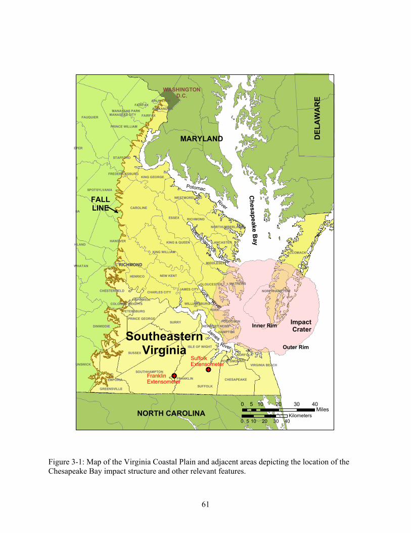
Figure 3-1: Map of the Virginia Coastal Plain and adjacent areas depicting the location of the Chesapeake Bay impact structure and other relevant features.
61
SA
SUSSEX
FAUQUIER
CAROLINE
HANOVER
DINWIDDIE
FAIRFAX
UNSWICK
SUFFOLK
ESSEX
E
SURRY
SOUTHHAMPTON
EPER
ACCOMACK
CHESTERFIELD
SPOTSYLVANIA
HENRICO
STAFFORD
CHESAPEAKE
WHATAN
KING & QUEEN
HLAND
ISLE OF WIGHT
YORK
GREENSVILLE
PRINCE WILLIAM
NEW KENT
KING WILLIAM
VIRGINIA BEACH
RICHMOND
PRINCE GEORGE
GLOUCESTER
WESTMORELAND
CHARLES CITY
KING GEORGE
JAMES CITY
MIDDLESEX
LANCASTER
NORTHHAMPTON
NORTHUMBERLAND
MATHEWS
RICHMOND
NORFOLK
HAMPTON
NEWPORT NEWS
ARLINGTON
PETERSBURG
POQUOSON
PORTSMOUTH
ALEXANDRIA
FAIRFAX
HOPEWELL
FRANKLIN
COLONIAL HEIGHTS
WILLIAMSBURG
FREDERICKSBURG
EMPORIA
MANASSAS CITYMANASSAS PARK
NORTH CAROLINA
MARYLAND DEL
AW
AR
EImpact Crater
Chesapeake B
ay
FALLLINE
SoutheasternVirginia
JamesRiver
River
Potomac
Outer Rim
Inner Rim
YorkRiver
RappahannockRiver
!C!C
Franklin Extensometer
Suffolk Extensometer
WASHINGTOND.C.
0 10 20 30 405Miles
0 10 20 30 405Kilometers

Figure 3-2: Correlation of hydrogeologic and stratigraphic units in southeastern Virginia. Modified from Meng and Harsh (1988), Hamilton and Larson (1988), and Powars (2000).
62
Period Epoch Geologic Units Hydrogeologic UnitsHolocene Holocene Deposits Quaternary Pleistocene Pleistocene Deposits
Columbia Aquifer
Bacons Castle Formation
Yorktown Confining Unit
Pliocene
Yorktown Formation
Yorktown-Eastover Aquifer
Eastover Formation St. Marys
Confining Unit St. Marys Formation Choptank Formation
St. Marys-Choptank Aquifer
Calvert Formation
Calvert Confining Unit
Miocene
Oligocene
Ches
apea
ke G
roup
Old Church Formation
Piney Point Aquifer
Chickahominy Formation (Crater)
Chickahominy Confining Unit
Piney Point Formation
Piney Point Aquifer
Nanjemoy Formation
Eocene
Marlboro Clay
Nanjemoy-Marlboro Confining Unit
Aquia Formation Aquia Aquifer
Brightseat Confining Unit
Tertiary
Paleocene
Pam
unke
y G
roup
Brightseat Formation Brightseat Aquifer
Peedee Confining Unit
Peedee Formation (of North Carolina)
Peedee Aquifer Red Beds (Powars, 2000)
Virginia Beach Confining Unit
Glauconitic Sands (Powars, 2000)
Virginia Beach Aquifer Upper Potomac Confining Unit
Upper Cenomanian Beds (Powars, 2000)
Late Cretaceous
Upper Potomac Aquifer Middle Potomac Confining Unit Middle Potomac Aquifer Lower Potomac Confining Unit
Cretaceous
Early Cretaceous Potomac Formation
Lower Potomac Aquifer
Jurassic-Triassic Rift-basin Rocks Paleozoic and Proterozoic Basement Rocks
= Not present in study area

Figure 3-3: Generalized geologic cross section of southeastern Virginia from the Fall Line to the coast. Modified from Powars and Bruce (1999), based on verbal communication with McFarland (2001).
63
Crystalline Basement
Potomac Formation
Cenomanian Beds
Red Beds
Aquia Formation
Yorktown FormationEastover Formation
Nanjemoy Formation
Quaternary DepositsBacons Castle Formation.
Glauconitic Sands
1000 ft
2500 ft
Sea Level
Saint Marys and Calvert Formations
Marlboro Clay
Delmarva-Old Church

Figure 3-4: Generalized hydrogeologic cross section of southeastern Virginia from the Fall Line to the coast (McFarland, 1998). Arrows show directions of groundwater flow under pre-development conditions.
64

Figure 3-5: Map showing the extent of the Lower Potomac aquifer with elevation of unit top in feet. Modified from Meng and Harsh (2000), Hamilton and Larson (1988), and Focazio and Samsel (1993).
65
-400
-800
-200
-10 00
-1200
-1400
-1800-2000
-2200-2400
-140
0
-1600
-40-40
NORTH CAROLINA
MARYLAND
DEL
AW
AR
E
Impact Crater
Chesapeake BayFALLLINE
SoutheasternVirginia
JamesRiver
River
Potomac
Outer Rim
Inner Rim
YorkRiver
RappahannockRiver
!C!C
Franklin Extensometer
Suffolk Extensometer
0 10 20 30 405Miles
0 10 20 30 405Kilometers
Note: Hydrogeologic interpretations pre-date impact crater discovery.

Figure 3-6: Map showing the extent of the Middle Potomac aquifer with elevation of unit top in feet. Modified from Meng and Harsh (2000), Hamilton and Larson (1988), and Focazio and Samsel (1993).
66
-200
-800
-40 0
-600
-100
0
- 12 00-1400
-160
0
-180
0
- 2000
0
NORTH CAROLINA
MARYLAND
DEL
AW
AR
E
Impact Crater
Chesapeake B
ayFALLLINE
SoutheasternVirginia
JamesRiver
River
Potomac
Outer Rim
Inner Rim
YorkRiver
RappahannockRiver
!C!C
Franklin Extensometer
Suffolk Extensometer
0 10 20 30 405Miles
0 10 20 30 405Kilometers
Note: Hydrogeologic interpretations pre-date impact crater discovery.

Figure 3-7: Map showing the extent of the Upper Potomac aquifer with elevation of unit top in feet. Modified from Meng and Harsh (2000), Hamilton and Larson (1988), and Focazio and Samsel (1993).
67
-400-6
00-8
00
-200
-100
0
0
-1200
-140
0
-140
0
-1400
-200
-400
-600
0
-120
0-100
-200
NORTH CAROLINA
MARYLAND
DEL
AW
AR
E
Impact Crater
Chesapeake B
ayFALLLINE
SoutheasternVirginia
JamesRiver
River
Potomac
Outer Rim
Inner Rim
YorkRiver
RappahannockRiver
!C!C
Franklin Extensometer
Suffolk Extensometer
0 10 20 30 405Miles
0 10 20 30 405Kilometers
Note: Hydrogeologic interpretations pre-date impact crater discovery.
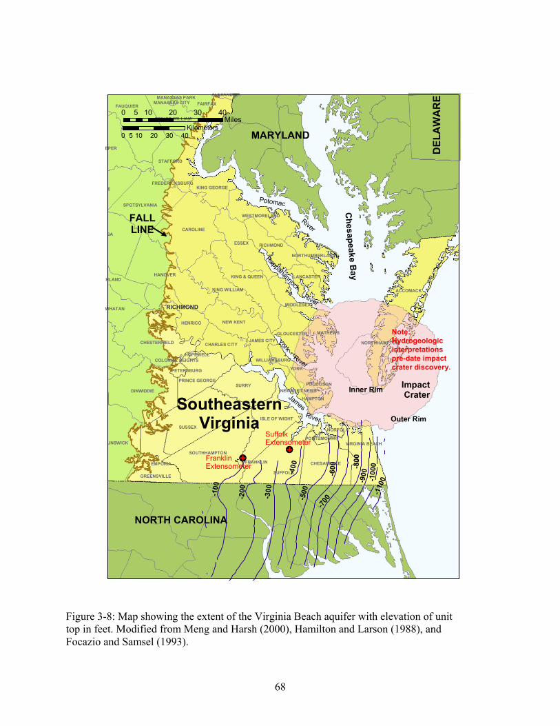
Figure 3-8: Map showing the extent of the Virginia Beach aquifer with elevation of unit top in feet. Modified from Meng and Harsh (2000), Hamilton and Larson (1988), and Focazio and Samsel (1993).
68
SA
SUSSEX
FAUQUIER
CAROLINE
HANOVER
DINWIDDIE
FAIRFAX
UNSWICK
SUFFOLK
ESSEX
E
SURRY
SOUTHHAMPTON
EPER
ACCOMACK
CHESTERFIELD
SPOTSYLVANIA
HENRICO
STAFFORD
CHESAPEAKE
WHATAN
KING & QUEEN
HLAND
ISLE OF WIGHT
YORK
GREENSVILLE
PRINCE WILLIAM
NEW KENT
KING WILLIAM
VIRGINIA BEACH
RICHMOND
PRINCE GEORGE
GLOUCESTER
WESTMORELAND
CHARLES CITY
KING GEORGE
JAMES CITY
MIDDLESEX
LANCASTER
NORTHHAMPTON
NORTHUMBERLAND
MATHEWS
RICHMOND
NORFOLK
HAMPTON
NEWPORT NEWS
PETERSBURG
POQUOSON
PORTSMOUTH
ALEXANDRIA
HOPEWELL
FRANKLIN
COLONIAL HEIGHTS
WILLIAMSBURG
FREDERICKSBURG
EMPORIA
MANASSAS CITYMANASSAS PARK
-70
0-6
00
-500-200
-800
-300
-900-4
00
-100 -110
0-100
0
NORTH CAROLINA
MARYLAND
DEL
AW
AR
E
Impact Crater
Chesapeake B
ayFALLLINE
SoutheasternVirginia
JamesRiver
River
Potomac
Outer Rim
Inner Rim
YorkRiver
RappahannockRiver
!C!C
Franklin Extensometer
Suffolk Extensometer
0 10 20 30 405Miles
0 10 20 30 405Kilometers
Note: Hydrogeologic interpretations pre-date impact crater discovery.

Figure 3-9: Map showing the extent of the Peedee aquifer with elevation of unit top in feet. Modified from Meng and Harsh (2000), Hamilton and Larson (1988), and Focazio and Samsel (1993).
69
-500
-400
-600
-700
-800
-300
-900
NORTH CAROLINA
MARYLAND
DEL
AW
AR
E
Impact Crater
Chesapeake BayFALLLINE
SoutheasternVirginia
JamesRiver
River
Potomac
Outer Rim
Inner Rim
YorkRiver
RappahannockRiver
!C!C
Franklin Extensometer
Suffolk Extensometer
0 10 20 30 405Miles
0 10 20 30 405Kilometers
Note: Hydrogeologic interpretations pre-date impact crater discovery.

Figure 3-10: Map showing the extent of the Aquia aquifer with elevation of unit top in feet. Modified from Meng and Harsh (2000), Hamilton and Larson (1988), and Focazio and Samsel (1993).
70
0
- 10 0 -200
-300
-400 -500
-600
-700
-800
-900
205
0
-500
-400
-600
-700
NORTH CAROLINA
MARYLAND
DEL
AW
AR
E
Impact Crater
Chesapeake B
ayFALLLINE
SoutheasternVirginia
JamesRiver
River
Potomac
Outer Rim
Inner Rim
YorkRiver
RappahannockRiver
!C!C
Franklin Extensometer
Suffolk Extensometer
0 10 20 30 405Miles
0 10 20 30 405Kilometers
Note: Hydrogeologic interpretations pre-date impact crater discovery.

Figure 3-11: Map showing the extent of the Chickahominy-Piney Point aquifer with elevation of unit top in feet. Modified from Meng and Harsh (2000), Hamilton and Larson (1988), and Focazio and Samsel (1993).
71
0
-100
-20 0
-300
-400
-500
-700
-800
-600
-900
-100
0
0
NORTH CAROLINA
MARYLAND
DEL
AW
AR
E
Impact Crater
Chesapeake BayFALLLINE
SoutheasternVirginia
JamesRiver
River
Potomac
Outer Rim
Inner Rim
YorkRiver
RappahannockRiver
!C!C
Franklin Extensometer
Suffolk Extensometer
0 10 20 30 405Miles
0 10 20 30 405Kilometers
Note: Hydrogeologic interpretations pre-date impact crater discovery.

Figure 3-12: Map showing the extent of the Saint Marys aquifer with elevation of unit top in feet. Modified from Meng and Harsh (2000), Hamilton and Larson (1988), and Focazio and Samsel (1993).
72
-500
-600
-700
-400
-300
-200
-300
-500
NORTH CAROLINA
MARYLAND
DEL
AW
AR
E
Impact Crater
Chesapeake BayFALLLINE
SoutheasternVirginia
JamesRiver
River
Potomac
Outer Rim
Inner Rim
YorkRiver
RappahannockRiver
!C!C
Franklin Extensometer
Suffolk Extensometer
0 10 20 30 405Miles
0 10 20 30 405Kilometers
Note: Hydrogeologic interpretations pre-date impact crater discovery.

Figure 3-13: Map showing the extent of the Yorktown-Eastover aquifer with elevation of unit top in feet. Modified from Meng and Harsh (2000), Hamilton and Larson (1988), and Focazio and Samsel (1993).
73
0
-50
55
-100
-1 5010
0
200
200
50
50
100
100
150
100
100
150
150
150
200
NORTH CAROLINA
MARYLAND
DEL
AW
AR
E
Impact Crater
Chesapeake BayFALLLINE
SoutheasternVirginia
JamesRiver
River
Potomac
Outer Rim
Inner Rim
YorkRiver
RappahannockRiver
!C!C
Franklin Extensometer
Suffolk Extensometer
0 10 20 30 405Miles
0 10 20 30 405Kilometers
Note: Hydrogeologic interpretations pre-date impact crater discovery.

IV: MEASUREMENTS AND ANALYSIS OF HYDROGEOLOGIC DATA FOR THE COASTAL PLAIN OF SOUTHEASTERN VIRGINIA
The analysis of land subsidence due to groundwater withdrawals requires the collection,
analysis, and synthesis of data from a variety of sources. Aquifer-system compaction measured
with extensometers is most meaningful in light of the water-level changes that induced the
compaction. Because these water-level changes are the result of withdrawals from the various
aquifers, measurement of withdrawals is necessary for an understanding of the relation between
pumpage and hydraulic heads.
A full analysis of aquifer-system compaction and land subsidence for the Coastal Plain of
Virginia would require an extensive database of withdrawals and water levels, as well as a three-
dimensional model. This approach is well beyond the scope of this research, but a large amount
of hydrogeologic data were necessary for this project simply to understand the compaction
behavior of this complex aquifer system in the vicinity of the extensometers. This section of the
document presents the data collected for this report in the Franklin and Suffolk areas, shown in
detail on the maps of figures 4-1 and 4-2. Included here are groundwater withdrawal data, water
level data, borehole data used for hydrogeologic interpretations. In addition, the extensometer
data are presented and analyzed.
Withdrawal Data
The accurate measurement and of withdrawals from the Coastal Plain aquifers in Virginia
is a very difficult undertaking. Reporting requirements vary by location across this region, and
by withdrawal category. In general, large industrial and municipal withdrawals are well known,
especially in regions designated by the Commonwealth of Virginia as groundwater management
areas, but agricultural withdrawals have not been quantified. Even less is known about domestic
withdrawals from private wells. The result of these disparities is a fairly large error in the
quantification of withdrawals. Fortunately, withdrawal information was not needed for in this
study for simulation of one-dimensional compaction, which relates aquifer-system compaction to
changes in hydraulic head. Even so, withdrawals were briefly considered for completeness and
for the purposes of comparison with measured compaction data.
Historically, groundwater withdrawals from the confined aquifers of the Virginia Coastal
Plain (figure 4-3) totaled less than 10 million gallons per day at the start of the twentieth century
74

and increased at a moderate rate prior to the World War II era (Kull and Laczniak, 1987).
Significant growth in population and industry in the Hampton Roads area at that time was
accompanied by increasing rates of withdrawal from many of the confined aquifers. Withdrawal
rates experienced increased tremendously in the 1950s and 1960s, due primarily to large
industrial and municipal withdrawals at a few large pumping centers. In the 1970s, the increase
in withdrawals began to level off as efforts were begun to limit new large wells in this region. A
regulatory approach adopted during that time continues to require proposed new wells in
designated groundwater management areas to be permitted based on their estimated impact on
the flow system. The permitting process, as well as new public water supply projects importing
surface water to the Hampton Roads area, helped to maintain relatively constant withdrawal rates
through the 1970s and 1980s. In the 1990s, however, growing demand for additional municipal
supplies led to the installation of new wells withdrawing brackish water from the Potomac
aquifers in the Hampton Roads area. These new withdrawals post-date the publication shown in
figure 4-3, but they represent noticeable increases in the withdrawal rates and have contributed to
additional declines in hydraulic head in southeastern Virginia.
The unusual distribution of withdrawals in the Coastal Plain of Virginia is perhaps more
interesting than their magnitudes, particularly with regard to the land subsidence problem.
Withdrawals from large industrial and municipal pumping centers dominate the Coastal Plain
system, in many cases even reversing the directions of regional groundwater flow. As a result,
total withdrawals are not evenly distributed across the region. The very skewed distribution of
withdrawal rates is depicted qualitatively in figure 4-4, which shows a raised-relief map of
withdrawals by county. In this figure, the large withdrawal rates from pulp and paper mills at
Franklin and West Point stand out very clearly from the withdrawals in all other areas. The 35 to
40 million gallons per day (mgd) at Franklin and 14 to 18 mgd at West Point together have
comprised almost half of the rate of measured withdrawals for the entire Coastal Plain of
Virginia in recent years (Harsh and Laczniak, 1987).
The consideration of all Coastal Plain withdrawals was well beyond the scope of the
present work, but withdrawals were examined on a more localized basis for the Franklin area. A
graph of the withdrawals near Franklin in recent years (figure 4-5) reveals that pumpage
magnitudes from the Middle and Lower Potomac aquifers differ somewhat, but the two records
exhibit similar patterns. It was initially expected that these withdrawals would vary seasonally,
75

but no seasonal pattern is evident in this graph. Instead, the industrial component overwhelms
any seasonal municipal or industrial component of the withdrawal record. Furthermore,
withdrawal data were available only from monthly reports, so the limited precision of this data
prohibited any quantitative comparison with the continuous compaction record. Instead, analysis
was focused on the effects of the withdrawals from these aquifers - their changing water levels -
which were generally available at better resolution and quantified with much greater confidence.
Hydraulic Head Data A thorough analysis of the water-level decline in the vicinities of Franklin and Suffolk
was a key component of this study. Interpretations of geologic and geophysical data indicated
that seven aquifers are present at each location, suggesting that a large amount of hydraulic head
data might be necessary to understand the vertical head distribution in this system. An ideal data
set, in fact, would have included water-level records for each of the seven aquifers at each of the
two locations from pre-development conditions through the present. The availability of actual
data was less than ideal, but an effort was made to identify and compile all of the water-level
records collected near the two sites over the history of measurement. A search of the USGS
Ground Water Site Inventory (GWSI) database yielded six records for the Franklin area and
eight records for the Suffolk area. These records are presented in figures 4-6 and 4-7.
The Franklin water levels presented in figure 4-6 include the following wells: (a) 55B62,
screened in the Yorktown-Eastover aquifer; (b) 55B67, screened in the Piney Point aquifer; (c)
55B16, screened in the Middle Potomac aquifer; (d) 55B22, screened in the Middle Potomac
aquifer; (e) 55B35, screened in the Middle Potomac aquifer; and (f) 55B36, screened in the
Lower Potomac aquifer. The location of these wells is presented in figure 4-1, and basic data on
well dimensions are presented in table 4-1. Each of the water level records is presented with a
graph scaled to maximize visibility, so it should be noted that the time (x axis) and hydraulic
head (y axis) scales do not match among the 6 graphs. There was no common scale on which
these records could reasonably be presented.
76

77
Table 4-1: Wells near the Franklin extensometer
Well ID Well Elevation (ft above mean sea level)
Screen Interval (ft below land surface)
Aquifer Designation Lateral Distance from Extensometer (ft)
55B62 27 25 – 30 Yorktown-Eastover 0
55B67 34 130 – 140 Piney Point 8,484
55B16 25 285 – 305 Middle Potomac 218
55B22 21 335 – 354 Middle Potomac 3,262
55B35 32 430 – 623 Middle Potomac 1,527
55B36 37 720 – 860 Lower Potomac 2,430
Two problems with these records are immediately obvious: (1) none of the records span
the complete history of water-level decline, and most do not span the same time periods, though
there is considerable overlap; and (2) few of the wells are located directly adjacent to the
extensometer, though most are located within about a mile of the instrument. These are important
issues because it was important to understand the history of water-level decline across the entire
period of groundwater development (essentially, the twentieth century), and these records were
collected for comparison with measured aquifer-system compaction data from the Franklin
extensometer. For the later purpose, close proximity to the extensometer is most desirable. Of
course, not all of the aquifers present at this location are represented in these water-level records,
which is another constraint on the understanding of the system. The most complete story of
water-level changes at Franklin is available from well 55B22, which is located in close proximity
to the Franklin extensometer and was measured from approximately 1940 to 1990. This record
was very important to the analysis, but its utility was somewhat limited because it did not extend
through the last decade of the century.
The Suffolk water levels presented in figure 4-7 include the following wells: (a) 58B268,
screened in the unconfined Columbia aquifer; (b) 58B269, screened in the Piney Point aquifer;
(c) 58B270, screened in the Upper Potomac aquifer; (d) 58B271, screened in the Upper Potomac
aquifer; (e) 58C56, screened in the upper part of the Middle Potomac aquifer; (f) 58C53,
screened in the Middle Potomac aquifer; (g) 58B235, screened in the Middle Potomac aquifer;
and (h) 58B273, screened in the Middle Potomac aquifer. These wells can be located in figure
4-2, and basic data on their dimensions are given in table 4-2.

78
Table 4-2: Wells near the Suffolk extensometer
Well ID Elevation (ft) Screen Interval (ft) Aquifer Designation Distance from Extensometer (ft) 58B268 35 12 – 20 Columbia 16,124
58B269 35 350 – 360 Piney Point 16,124
58B270 35 490 – 500 Upper Potomac 16,124
58B271 29 501 – 710 Upper Potomac 16,124
58C56 10 557 – 567 upper Middle Potomac 0
58C53 10 881 – 896 Middle Potomac 0
58B235 53 530 – 562 Middle Potomac 10,389
58B273 26 541 – 640 Middle Potomac 15,108
The Suffolk water-level records are much less useful than the Franklin records, because
they are generally located much farther from the extensometer installation and generally span
much shorter time periods. In particular, none of the water-records available for Suffolk show
head decline across the early to middle parts of the twentieth century, though a few early data
points for the Middle Potomac aquifer are available from 58B235 (figure 4-7g). Consequently,
these water-level records by themselves provided little constraint on historical declines in water
levels at Suffolk.
In order to address the problems with limited time periods for the water level records at
both locations, early reports on groundwater conditions in Virginia were examined in detail.
Sanford (1913) and Cederstrom (1945) provided both early water-level measurements at nearby
locations and qualitative reports of approximate groundwater levels in the early part of the
century. These reports were used to supplement the available records to generate a
comprehensive understanding of the history of head decline at the two locations. Data from these
reports were ultimately used in the generation of synthetic water-level records for input files for
the compaction model.
From the inspection of water-level records at both sites, some important general
observations can be made. First, declines in water levels have been most dramatic in the Potomac
aquifers, and particularly in the Middle Potomac aquifer, which has experienced a head decline
76

79
of over 60 meters from pre-development conditions (figure 4-6d). The largest head declines in
the Potomac aquifers are apparent at the Franklin location, where the lowest hydraulic heads in
the Coastal Plain system have historically been measured (Cosner, 1975). On the other hand,
heads in the Potomac aquifers at Franklin have generally leveled off in recent years, with some
minor fluctuations.
It is clear that water-level declines in the Potomac aquifers have been less severe at
Suffolk, but the available records indicate that water levels are still declining significantly at
Suffolk. It is unclear whether these declines result from the expansion of the regional cone of
depression outward from the Franklin pumping center or from the increase in local pumping
rates, but it is possible that both factors are responsible. An examination of withdrawal data and
water-level records revealed that these drawdowns appear to represent the superposition of local
and regional effects.
There is a strong apparent correlation between the water levels in the various aquifers at
each site, particularly for the Potomac aquifers of Cretaceous age. It is not known whether this
correlation is controlled by concurrent pumping from all of the Potomac aquifers or from leakage
through the confining units, because many large wells are screened across two or three of the
Potomac aquifers. However, the apparent correlation between the Potomac water levels and the
water levels of the Piney Point aquifer (which is not pumped significantly at these locations)
indicates that significant downward leakage is occurring through the system. Comparison of
hydraulic heads indicates that flow at both sites likely has a strong vertical component (both
downward and upward) toward the Middle Potomac aquifer, likely driven by pumping.
Perhaps the most significant observation resulting from the water-level analysis is the
apparent effect of the confining unit(s) above the Potomac system, which has maintained a very
large head gradient between the Piney Point aquifer above and the Upper Potomac aquifer
below. At Franklin, this gradient is especially large, with almost 50 meters of head differential
between two wells, separated by less than 60 vertical meters between the two aquifers. It is also
notable that the Yorktown-Eastover aquifer and the unconfined Columbia aquifer show no
significant effects from pumping, and appear to be totally isolated from the aquifers below.
In addition to analyzing water levels in the vicinity of Franklin and Suffolk, a larger
effort was undertaken to understand the current head conditions in the Potomac system across the
Coastal Plain of Virginia by generating a current map of the piezometric surface for the Middle

80
Potomac aquifer. Water-level data for the Middle Potomac for aquifer for 1998 was available
from 15 observation wells across the eastern part of Virginia. These water levels were analyzed,
adjusted and contoured using geographic information system tools, resulting in the regional
water-level map that was presented in figure 1-2. With only 15 control points over a very large
area, this map is only an approximate representation of 1998 conditions, but it was useful
nonetheless. It revealed significant declines in head across much of the region from 1978
conditions (Hopkins and others, 1981), as well as an expansion of the regional cone of
depression northward toward Virginia’s Northern Neck and eastward toward the Chesapeake
Bay.
Extensometer Design and Installation
In an effort to learn more about the subsidence in the Coastal Plain resulting from
groundwater withdrawals, two compaction wells equipped with extensometers were installed in
Southeastern Virginia within a decade of the Holdahl and Morrison (1974) releveling report. The
first compaction well (55B60) was drilled at Franklin by the Virginia Water Control Board and
instrumented by the USGS in September 1979. The second compaction well (58C52) was drilled
and instrumented at Elephant Fork near Suffolk in June 1982. Both extensometers were
maintained by the USGS and provided continuous cumulative compaction data for the complete
aquifer system from the time of their installation until they were removed from service at the end
of 1995, due to funding constraints.
Internal USGS memos and progress reports provide information about the construction of
the compaction wells and extensometers. Both compaction wells penetrate the complete
sedimentary system, extending from land surface to bedrock. The Franklin well, located at an
elevation of 29 feet above mean sea level, has a total depth of 866 feet below land surface, or
837 feet below the sea level datum. The Suffolk well, with an elevation of 11.3 feet, has a total
depth of 1599 feet below land surface, or 1587.7 feet below sea level.
Aside from their depths, the compaction wells are of similar construction. Both wells
were drilled with the Virginia Water Control Board’s hydraulic rotary drilling rig using a 6.75-
inch bit. The wells are cased from surface to bedrock with steel casing of 4 inches in diameter,
connected with threaded joints and couplings. A 10-foot section of screen is located 5 feet from
the bottom of each casing. The annular space between the casing and the borehole of each well is

81
filled with well cuttings, except for the upper 20 feet, which is grouted with cement. The
extensometer pipe for each well, which varies in diameter from 1.5 to 2 inches, is installed inside
the casing and cemented in bedrock at the bottom of the well. The extensometer pipe extends
from bedrock to above land surface, providing a stable reference point for measuring changes in
the total thickness of the Coastal Plain aquifer system at each site. The vertical displacement of
the top of the reference pipe relative to a reference platform at land surface is equal to the
compaction or expansion of the aquifer system between the bedrock anchor and the base of the
platform. Each of the two platforms is constructed of steel plate and is mounted on three legs.
The legs are constructed of 1.5-inch steel pipes driven to refusal at approximately 20 feet below
land surface, inside 4-inch plastic pipes installed in auger holes that extend to the water table.
This platform installation is designed to minimize temperature and moisture effects occurring
near land surface in order to better isolate and measure compaction and expansion within the
aquifer system. A counter-weighted lever attached to the top of each reference pipe places the
pipe in tension in order to reduce frictional contact between the pipe and the well casing, the
greatest source of error for this type of instrument.
To record the compaction or expansion, a modified Stevens “Type F” recorder mounted
on the reference platform is attached to the top of the extensometer pipe. A gear amplifies the
movement of the recorder pen in order to provide a record with greater sensitivity to small
changes in thickness. At Suffolk, the gear ratio for the recorder provides the standard
amplification of 15:1, while the gear ratio at Franklin provides an amplification of 50:1, yielding
greater sensitivity. Both recorders supplied continuous analog records of the cumulative
compaction at the two sites in the form of monthly data charts from the time of their installation
through the end of 1995. A schematic diagram of the extensometer setup is provided in figure 4-
8, and photographs of the instruments are provided in figure 4-9.
Pipe extensometer installations similar to those described here have been used to
successfully measure compaction at many other sites (Poland et al., 1984). This technique is
considered to be one of the most accurate methods available for measuring compaction, with a
resolution of 3.0 x 10⁻⁴ meters (Hanson, 1989), and it can be effectively employed to depths of
750 to 1000 meters under favorable conditions (Poland and others, 1984).
82
Borehole Data U.S. Geological Survey staff used borehole geophysical data from the Franklin and
Suffolk sites, in conjunction with local geologic data, to identify the geologic and hydrogeologic
units present at the locations of interest. Cuttings and electrical logs were obtained from the
extensometer boreholes during their installation, and interpretations of these logs were assembled
into diagrams for Franklin (figure 4-10) and Suffolk (figure 4-11). A thorough description of the
techniques used to interpret these logs is available in a USGS report on borehole geophysics
(Keys, 1990).
Extensometer/Compaction Data
Measurements from the compaction recorders were collected in the form of monthly strip
charts with continuous pen records. These collected charts were marked and calibrated to
account for monthly change-overs of the charts, and the complete record was then manually
digitized for each of the two sites. The digital records of compaction were then adjusted to
remove the magnification provided by the gear ratios of the instruments at Franklin (50:1) and
Suffolk (15:1), resulting in measurements of the compaction. After initial examination and
archival of the raw digital record, it was filtered to produce a working record with a more
manageable number of data points.
Although the chart records are not shown here, they reveal some information less
apparent in the digital record but worthy of discussion. The raw charts show the effect of down-
hole friction on the compaction measurements. It is known from many other experiments with
borehole pipe extensometers that the measurement pipe often comes into some contact with the
well casing. When this happens, friction may cause the instrument to record step changes in
strain rather than a smooth record. The extensometer counterweight is designed to remove most
of this frictional component, but small steps were still apparent in the record. The effects of the
step changes are small enough to only minimally affect the measured compaction, but the role of
friction as a source of error should be acknowledged.
The digital records of measured compaction at Franklin and Suffolk are plotted in figure
4-12. These extensometer records reveal the changes in magnitude and rate of compaction in the
entire aquifer system at the two sites. At Franklin, 24.2 millimeters of compaction was measured

83
from September of 1979 to December of 1995, for an average rate of approximately 1.5 mm/yr.
At Suffolk, 50.2 mm of compaction was measured from June of 1982 to December of 1995, for
an average rate of 3.7 mm/yr.
It is perhaps initially surprising that measured compaction at Suffolk was twice as large
as that at Franklin, which has experienced declines in head over 30 meters greater. However,
comparison with other site data reveals some probable reasons for this relation. First, the depths
of the extensometer boreholes shows that the aquifer system at Suffolk (1599 ft, 487.4 m) is
almost double the Franklin thickness (866 ft, 269.9 m), so there is twice as much material to
undergo compaction. A similar relation is apparent for the thickness of fine-grained confining
units and aquitards, which total 62.7 m in thickness at Franklin and 130.8 m at Suffolk.
Furthermore, inspection of the water level records for the two sites indicates that while water
levels in the Potomac aquifers at Franklin were relatively stable over the period of compaction
measurement, water levels continued to decline at Suffolk over the same period.
The other difference between the Franklin and Suffolk records is the magnitude of the
observed short-term compaction and expansion events. Short-term water-level fluctuations seem
to be expressed much more clearly in the compaction record at Franklin as compared to Suffolk.
Much of this difference is probably the result of greater instrumental error at Suffolk. The
expected greater error at Suffolk is the result of two factors that would both be expected to affect
the sensitivity of the instrument: a lower gear ratio and a deeper borehole. A lower gear ratio
affects the ability of the extensometer to transmit small changes in strain to the recorder, while a
deeper borehole results in greater potential for friction in the borehole and hampers the ability of
the instrument to respond to small changes in vertical strain in the aquifer system.
At Franklin, short-term compaction and expansion of the aquifer system correlates very
well with observed changes in hydraulic head in the Potomac aquifers. A comparison of these
records (figure 4-13) shows that episodes of measured aquifer-system compaction closely
followed head declines, and head recovery was followed by measured expansion of the aquifer
system. At these short-term (hours to days) time scales, the responses likely express the
recoverable (elastic) compaction and expansion of the coarse-grained aquifer units rather than
compaction of fine-grained intervals, which is usually characterized by a delayed response.
The compaction response at Suffolk was similar with regard to these short-term events,
but less distinct. Short-term head declines in the Potomac aquifers resulted in some additional
84
measured compaction, but head recovery resulted in very little if any expansion of the system.
There are two possible reasons for this effect. Instrument error, discussed previously, may have
prevented very small changes in aquifer-system strain from being expressed in the measured
record. These millimeter-scale changes in the system are close to the resolution limit of this type
of instrument even under ideal conditions (F.S. Riley, USGS, oral communication, 2001).
Another possibility is that short-term head changes expressed in a given water-level record do
not accurately reflect the head conditions throughout all the coarse-grained portion of the system.
Pumping at Suffolk is confined to a relatively small vertical section of the system, unlike
Franklin, where large wells are screened across large intervals of the various aquifers. Thus,
heads expressed in the Potomac records may not be occurring throughout the system, though the
best available water-level records (figure 4-7e,f) indicate that changes are occurring over
significant vertical distances. From the available knowledge of the system, instrument precision
seems likely to be the cause of the differences in the measured compaction responses at the
Franklin and Suffolk sites.
While short-term correlations are apparent between compaction and water levels at both
sites, relations between long-term trends in stress and strain are much less clear. As figure 4-13
demonstrates, cumulative compaction continues to increase even during periods of short-term
water-level recovery, and the trend of the compaction record shows a relatively consistent
increase in compaction with time even though the water levels at Franklin show very little long-
term head decline. At Suffolk, hydraulic heads declined more consistently and at a greater rate
over the period of the extensometer record, providing a possible cause for the dominant trend of
increasing compaction versus time.
Greater rates of compaction at Franklin during 1987 and 1990 (figure 4-12) are notable
because of their relation to head declines in the Potomac aquifers. The increased compaction rate
during these times appears to accompany the decline in the Middle Potomac water level beyond
the past maximum drawdown. It seems likely, then, that this type of response over intermediate
time periods (months to years) reflects some non-recoverable (inelastic) compaction of confining
units and aquitards, particularly in the Potomac system.
This analysis still does not explain the dominant trend of increasing compaction over the
complete extensometer record. The very consistent overall trends for both the Franklin and
Suffolk records are characteristic of long-term delayed drainage from fine-grained units,
85
resulting in slow but steady compaction of the system. Riley (1969) demonstrated a useful
method for analyzing the compaction response by plotting strain (compaction) versus stress
(hydraulic head). Using field data, Riley showed that estimates for recoverable and
nonrecoverable skeletal storage coefficients can be calculated from strain-stress plots. The
skeletal storage coefficient Sk is defined as the change in thickness (∆b) divided by the change in
effective stress (∆σe), so Sk can be calculated from the inverse of the slope of the change in
measured compaction versus the measured head change (Riley, 1969). A number of authors have
shown that head changes that do not exceed past maximum levels typically cause the elastic
response of the aquifer system, which appears on strain-stress plots as hysteresis loops
characterized by a constant slope (Epstein, 1987, Sneed and Galloway, 2000). On the other hand,
head changes beyond the past maximum cause an inelastic response, which appears on strain-
stress plots as a dominant linear trend.
Applying Riley’s (1969) method to the data from the Franklin location resulted in the
graph in figure 4-14, with measured compaction on the x axis and the Middle Potomac water
level on the y axis. In this case, a fairly consistent elastic response (dashed red lines) yielded
approximate Ske values of 5 x 10⁻⁴ for the system as a whole. On the other hand, no dominant
trend can be discerned across the total record. The absence of a trend that would define Skv
indicates that the nonrecoverable (inelastic) behavior of this system is not characterized by a
single strain-stress relation. This is not particularly surprising in hindsight, because both the
Franklin and Suffolk extensometers measure total strain (compaction) over hundreds of vertical
feet of very heterogeneous materials.
In fact, Riley’s method has been most successfully applied in aquifer systems
conceptually more simple than that of the Virginia Coastal Plain. In the Coastal Plain system, it
is known that the vertical stress variations in the system are quite large. Furthermore, available
geologic evidence indicates that the units of this system would be expected to exhibit very
different hydrogeologic behaviors. In general, the large degree of vertical heterogeneity in this
system limited the utility of Riley’s method and required the use of a more complicated
compaction model to characterize the system and explain the strain-stress relation.
The necessity of a more complex model was made even more apparent by the application
of a number of statistical methods, such as correlation analysis, to the problem of describing the
strain-stress response. Very close correlations between specific water-level records and the total

86
compaction record might have enabled the measured strain to be attributed to specific stress
events in individual aquifers. Overall, these statistical methods were largely inconclusive and
ineffectual, probably because they could not account for long-term delayed compaction
responses from slowly draining fine-grained units.
Similarly, an attempt was made to quantify elastic and inelastic storage coefficients by
separating short-term and long-term trends in the data, as demonstrated by Sneed and Galloway
(2000). Ideally, removing a long-term trend due to time-dependent nonrecoverable compaction
would allow short-term elastic compaction to be calculated independently. However, applying
this technique to the Coastal Plain data revealed that compaction in this system could not be
separated into only two distinct trends. Instead, this exercise provided further evidence that
cumulative compaction in this system is the result of compaction in a number of different units
with distinct patterns of time-dependent compaction resulting from different hydrologic
characteristics and different stress conditions.
By itself, the compaction record developed from the extensometer data is of limited
utility in describing historical aquifer-system compaction and land subsidence in this region,
because the measurements span so little of the history of groundwater development. To provide a
rough estimation of total historical subsidence, the extensometer data (available for1979 – 1995)
was supplemented with available data on the subsidence of benchmarks (available for 1940-
1971) (Holdahl and Morrison, 1974), and interpolation was used to fill in the gaps in this
assembled record. This process resulted in estimates for total subsidence at Franklin and Suffolk
from predevelopment conditions, presented in table 4-3.
Table 4-3: Estimated total subsidence in southeastern Virginia Franklin Subsidence (mm) Suffolk Subsidence (mm)
Prior to 1940 < 10 Prior to 1940 0
1940 - 1971 81 1940 - 1971 62
1971 - 1979 ~ 21 1971 - 1982 ~ 22
1979 - 1995 24.2 1982 - 1995 50.2
Total 1900 - 1995 ~ 136.2 Total 1900 - 1995 ~ 134.2

87
While the estimates indicate that the total amount of subsidence at the two locations is almost
identical, much more of the total subsidence at Suffolk has occurred over the last two decades,
probably because water levels have continued to decline at that location, while water levels near
Franklin have remained nearly constant during the same period.

Figure 4-1: Detailed map of the Franklin, Virginia area. Wells are designated by USGS local identification numbers, with aquifer designations in parentheses. (Base map from the USGS 7.5’ Quadrangle.
88
55B 35 (MP)55B 36 (LP)
Compaction Well(55B 60)55B 16 (MP)
55B 22 (MP)
55B 62 (YE)
55B 67 (PP)
76°54’76°55’76°56’76°57’
36°42’36°41’
36°40’
1 mile2000 4000feet
1 kilometer500meters

Figure 4-2: Detailed map of the Suffolk, Virginia area. Wells are designated by USGS local identification numbers, with aquifer designations in parentheses. (Base map from the USGS 7.5’ Quadrangle.
89
76°35’ 76°34’76°36’76°37’
36°45’
36°44’
36°43’
58C 53 (MP)58C 56 (UMP)
58B269 (PP)58B268 (CO)
58B270 (UP)
58B271 (UP)
58B273 (MP)
Compaction Well(58C 52)
58B235 (MP)
1 mile2000 4000feet
1 kilometer500meters

Figure 4-3: Historical record of yearly withdrawals (in millions of gallons per day) from the confined aquifers of the Virginia Costal Plain.
90
0
10
20
30
40
50
60
Wit
hdr
awal
s (m
gd)
19401920 198019601900
Middle PotomacMiddle Potomac
Upper PotomacUpper Potomac
Lower PotomacLower Potomac

Figure 4-4: Diagram showing the magnitude and distribution of groundwater withdrawals from the confined aquifers in the Virginia Coastal Plain. Contours are in increments of million gallons per day (mgd). Large peaks are due to industrial withdrawals at Franklin to the south (left) and West Point to the north (right).
91
Franklin~35 mgd
West Point~15 mgd

Figure 4-5: Monthly groundwater withdrawals (in millions of gallons) at Franklin from 1982 through 1995 for the Lower Potomac (LP), Middle Potomac (MP), Upper Potomac (UP) and Aquia (AQ) aquifers.
92
0
200
400
600
800
1000
1200
J-82 J-83 J-84 D-84 J-86 J-87 J-88 D-88 J-90 J-91 J-92 D-92 J-94 J-95
Date
Mon
thly
With
draw
als
(Mill
ions
of G
allo
ns)
MP
LP
TOTAL

Figure 4-6 a-b: Water levels from available monitoring wells in the Franklin, Virginia area, in meters relative to the sea-level datum. Records are designated by USGS local identification numbers.
93
Fig. 4-6a
1980 1990 2000Year
2
3
4
5
6
Wat
er L
evel
(met
ers
rela
tive
to s
ea le
vel)
55B62 (YORKTOWN-EASTOVER AQUIFER)
Fig. 4-6b
1985 1995Year
-2
-1
0
1
2
Wat
er L
evel
(m
eter
s re
lativ
e to
sea
leve
l)
55B67 (PINEY POINT AQUIFER)

Figure 4-6 c-d: Water levels from available monitoring wells in the Franklin, Virginia area, in meters relative to the sea-level datum. Records are designated by USGS local identification numbers.
94
Fig. 4-6c
1960 1970 1980 1990 2000Year
-70
-60
-50
-40
-30
-20
Wat
er L
evel
(m
eter
s re
lativ
e to
sea
leve
l)
55B16 (MIDDLE POTOMAC AQUIFER)
1940 1950 1960 1970 1980 1990 2000Year
-60
-50
-40
-30
-20
-10
0
10
Wat
er L
evel
(m
eter
s re
lativ
e to
sea
leve
l)
55B22 (MIDDLE POTOMAC AQUIFER)
Fig. 4-6d

Figure 4-6 e-f: Water levels from available monitoring wells in the Franklin, Virginia area, in meters relative to the sea-level datum. Records are designated by USGS local identification numbers.
95
Fig. 4-6e
1965 1975 1985 1995Year
-60
-50
-40
-30
-20W
ater
Lev
el (
met
ers
rela
tive
to s
ea le
vel)
55B35 (MIDDLE POTOMAC AQUIFER)
Fig. 4-6f
1970 1980 1990 2000Year
-60
-50
-40
-30
-20
Wat
er L
evel
(m
eter
s re
lativ
e to
sea
leve
l)
55B36 (LOWER POTOMAC AQUIFER)

Figure 4-7 a-b: Water levels from available monitoring wells in the Suffolk, Virginia area, in meters relative to the sea-level datum. Records are designated by USGS local identification numbers.
96
Fig. 4-7a
1980 1990 2000Year
5
6
7
8
9
10W
ater
Lev
el (
met
ers
rela
tive
to s
ea le
vel)
58B268 (COLUMBIA AQUIFER)
Fig. 4-7b
1980 1990 2000Year
-10
-8
-6
-4
-2
0
2
Wat
er L
evel
(m
eter
s re
lativ
e to
sea
leve
l)
58B269 (PINEY POINT AQUIFER)
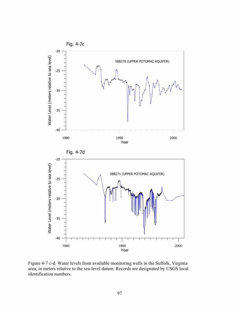
Figure 4-7 c-d: Water levels from available monitoring wells in the Suffolk, Virginia area, in meters relative to the sea-level datum. Records are designated by USGS local identification numbers.
97
Fig. 4-7c
1980 1990 2000Year
-40
-35
-30
-25
-20W
ater
Lev
el (
met
ers
rela
tive
to s
ea le
vel)
58B270 (UPPER POTOMAC AQUIFER)
Fig. 4-7d
1980 1990 2000Year
-40
-35
-30
-25
-20
Wat
er L
evel
(m
eter
s re
lativ
e to
sea
leve
l)
58B271 (UPPER POTOMAC AQUIFER)
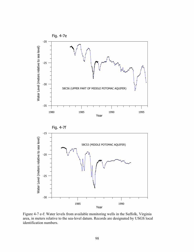
Figure 4-7 e-f: Water levels from available monitoring wells in the Suffolk, Virginia area, in meters relative to the sea-level datum. Records are designated by USGS local identification numbers.
98
Fig. 4-7e
1980 1985 1990 1995Year
-35
-30
-25
-20W
ater
Lev
el (
met
ers
rela
tive
to s
ea le
vel)
58C56 (UPPER PART OF MIDDLE POTOMAC AQUIFER)
Fig. 4-7f
1985 1990Year
-30
-25
-20
-15
Wat
er L
evel
(m
eter
s re
lativ
e to
sea
leve
l)
58C53 (MIDDLE POTOMAC AQUIFER)

Figure 4-7 g-h: Water levels from available monitoring wells in the Suffolk, Virginia area, in meters relative to the sea-level datum. Records are designated by USGS local identification numbers.
99
Fig. 4-7g
1900 1910 1920 1930 1940 1950 1960 1970 1980 1990 2000Year
-40
-30
-20
-10
0
10
20W
ater
Lev
el (
met
ers
rela
tive
to s
ea le
vel)
58B235 (MIDDLE POTOMAC AQUIFER)
Fig. 4-7h
1980 1990 2000Year
-50
-40
-30
-20
Wat
er L
evel
(m
eter
s re
lativ
e to
sea
leve
l)
58B273 (MIDDLE POTOMAC AQUIFER)

Figure 4-8: Schematic diagram of extensometer instrument.
100
Extensometer Pipe
Well Casing
Bottom of extensometer pipe anchored in bedrock
ThreadedRod
AdjustingNut
Steel Tape
CompactionRecorder
Steel Table
Weights
H-BeamFulcrum Arm
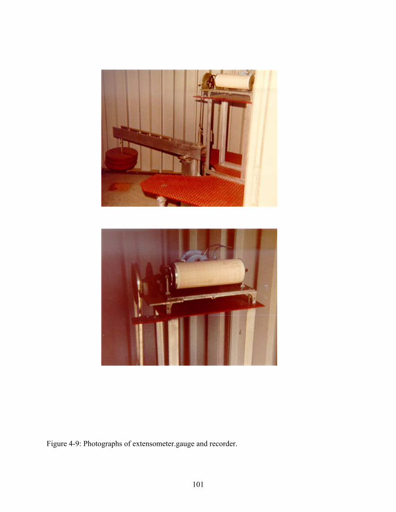
Figure 4-9: Photographs of extensometer.gauge and recorder.
101
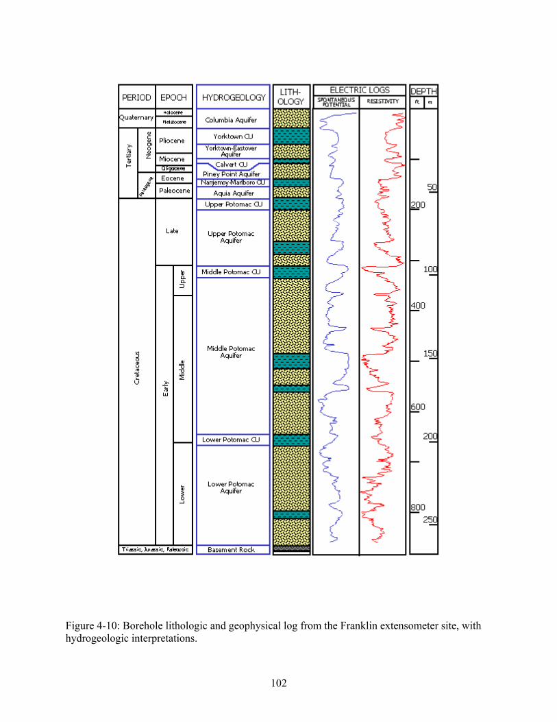
Figure 4-10: Borehole lithologic and geophysical log from the Franklin extensometer site, with hydrogeologic interpretations.
102

Figure 4-11: Borehole lithologic and geophysical log from the Suffolk extensometer site, with hydrogeologic interpretations.
103
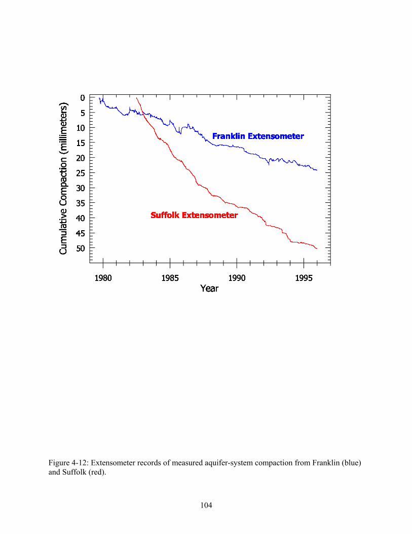
Figure 4-12: Extensometer records of measured aquifer-system compaction from Franklin (blue) and Suffolk (red).
104

Figure 4-13: Comparison of Franklin compaction record with water levels in the Lower and Middle Potomac aquifers. Water levels units are meters below sea-level datum. Compaction units are millimeters of cumulative compaction since beginning of measured record (1979).
105
1980 1985 1990 1995 2000
30
25
20
15
10
5
0
Tota
l Cu
mu
lati
ve C
ompa
ctio
n (
mm
)
60
55
50
45
40
35
30
Wat
er L
evel
(m
eter
s b
elow
sea
leve
l)
COMPACTION
LOWER POTOMAC AQUIFER
MIDDLE POTOMAC AQUIFER

Figure 4-14: Graph of strain (meters of water) versus stress (mm of compaction) at Franklin area. Dashed lines show slopes of recoverable compaction loops.
106
46
48
50
52
54
56
58
-2 0 2 4 6 8 10 12 14 16 18 20 22 24 26
Wat
er L
evel
s (m
)
Compaction (mm)

V: ONE-DIMENSIONAL SIMULATION OF COMPACTION IN SOUTHEASTERN VIRGINIA
Because of the complexity of the Coastal Plain aquifer system, a numerical model was
needed to account for vertical variations in applied stress across numerous hydrogeologic units,
characterize the resulting time-dependent vertical variations in strain, and discern the
contributions of individual hydrogeologic units to the total observed compaction. The one-
dimensional finite-difference numerical model (COMPAC) developed by Helm (1975, 1976b)
was chosen because it has been well documented and has been sucessfully used to simulate
compaction in systems similar to that presented here (Epstein, 1987; Hanson, 1989). The
COMPAC model uses the diffusion equation to calculate the time distribution of compaction in a
hydrogeologic unit from the history of applied stress on the upper and lower boundary of the
unit, as well as the unit’s properties of vertical hydraulic conductivity, specific storage
(recoverable and nonrecoverable), and thickness. Each Coastal Plain hydrogeologic unit was
simulated separtately, but evaluation of the parameters of each unit was achieved by matching
the sum of the simulated compaction in all units to the measured cumulative compaction of the
complete system from extensometer data.
The relative simplicity of the COMPAC model is partly the result of the rather limited
computer resources available at the time of model development, but simplicity was an advantage
in this application because of the limited input and calibration data available. Despite its apparent
limitations, a one-dimensional model is appropriate for simulation of compaction because of
aquitard anisotropy (Helm, 1975). As Helm (1975) points out, vertical hydraulic conductivity is
usually much smaller than horizontal hydraulic conductivity, which results in stresses acting in a
direction that is “essentially vertical.” This one-dimensional approach to simulation of aquifer-
system compaction due to groundwater withdrawals has been shown to produce very accurate
results in a number of cases (Epstein, 1987; Hanson, 1989).
Model Computation of Aquifer-System Compaction
The COMPAC model computes the transient vertical distribution of effective stress
within an idealized hydrogeologic unit from its known stress (water-level) history and the
hydraulic parameters K’, S’skv, and S’ske. From the effective stress distribution, the model
computes the resulting cumulative compaction and expansion with time at discrete horizontal
107

planes within the unit (Helm, 1975). The development of the computational approach used in the
model and outlined here were described in detail by Helm (1975, 1976b), and additional
insightful comments on Helm’s work were provided by Hanson (1989).
Helm (1975) pointed out that two relations are needed to compute compaction of an
aquitard or confining unit from known changes in applied stress at an aquitard or confining unit
boundary (i.e. in the aquifer): (1) the relation of internal effective stress to known boundary
stress, and (2) the relation between the internal stress distribution and compaction. For an
aquifer, it is assumed that changes in stress are instantaneously distributed throughout the
thickness of the unit, so only the second relation is needed.
The vertical distribution of effective stress in a homogeneous compacting layer can be
given by a linear partial differential equation (Scott, 1963):
2
2
'
'
zp
SK
ttp
s
T
∂∂
=
∂∂−
∂∂ σ
(5-1)
where
p is the pore water stress [N/m2],
σT is the total stress due to the weight of overlying materials [N/m2]
K’ is the vertical hydraulic conductivity of the compacting unit [m/d],
Ss’ is the specific storage of the compacting unit [m-1]
z is the vertical coordinate [m]
t is time
The rate of applied stress on the boundary of the vertically compacting layer is given by the
second term on the left side of the above equation. If it is assumed that the boundary
(overburden) stress is applied instantaneously at time zero and does not change, this term can be
simplified to Terzaghi’s formulation of the diffusion equation (Scott, 1963):
2
2
'
'
zp
SK
tp
s ∂∂
=
∂∂
(5-2)
This equation represents the distribution of pore pressure within the compacting unit. It can also
be written in terms of effective stress, σe, because if σT does not change, the change in effective
stress is equal but opposite to the change in the pore water stress (Helm, 1974):
108
2
2
'
'
zSK
te
s
e
∂∂
=
∂∂ σσ
(5-3)
Because the change in p is equal and opposite to the change in σe, the difference between them is
due only to a sign convention, and these two terms can be used interchangably for most
situations involving compaction due to water-level decline. Due to the assumption of no change
in σT, the formulations of Terzaghi and Helm presented above are less appropriate where the
change in effective stress results from factors other than the reduction of head in a confined
system (Hanson, 1989).
It should be mentioned that the compressibility term Ss’ in the above equations has two
components: one due to the compressibility of the granular skeleton (S’sk) and the other due to
the compressibility of water (S’sw), (Helm, 1975). Because it has been shown that water is
typically much less compressible than the skeleton (Scott, 1963), Helm chose to disregard the
S’sw component in his development of the model (Helm, 1975). However, in systems where S’sk
is small (such as the Coastal Plain of Virginia), the effect of water compressibility should not be
disregarded altogether.
As discussed in previous sections, the term for the skeletal compressibility, S’sk, has two
components as well, depending on the whether the current effective stress in an aquitard or
confining unit is above or below the past maximum (preconsolidation) level (Helm, 1975). When
σe is less than the past maximum, the skeleton responds in a recoverable (pseudo-elastic)
manner, and S’ske is the more appropriate term. When σe is greater than the past maximum, the
skeleton responds in a non-recoverable (inelastic) manner, and S’skv is the appropriate term. A
coarse-grained aquifer unit is assumed by the model to compact and expand elastically under all
stress conditions, so the appropriate aquifer storage/compressibility term is Sske (Hanson, 1989).
The COMPAC model uses a time-centered finite-difference numerical approximation
(Crank and Nicholson, 1947) of Helms’ effective stress equation (5-3) and an adaptation of the
Thomas algorithm, a forward and backward substitution method (Remson and others, 1971), to
calculate the transient stress distribution within an aquitard or confining unit and solve the set of
equations for the effective stress at each node for each time step (Helm, 1975). Compaction is
then computed with the following expression at each time step as the change in thickness (∆b’)
of a bed with total thickness (b0’) (Helm, 1975):
109

( ) (
∆+∆−∆+∆∆=∆ ∑ ∑
−
=
−
=++
1
1
1
11
'1
')5.0('J
j
J
j
nej
nejske
nvj
nvjskv ppSppSzb )
)
(5-4)
where
, 0max'max' jnj
nvj ppp −=∆
, nj
nj
nej ppp 'max' −=∆
∆b’ is the change in aquitard or confining unit thickness,
j is the total number of nodes in the unit,
j–1 is the total number of elements in the unit, with uniform mesh spacing ∆z
n is the time-step number,
p’nj is the effective stress at node j and time step n,
p’maxnj is the past maximum effective stress at node j and time step n.
At any node, when p’ is equal to p’max, the second (elastic) term in the brackets drops out, and
compaction occurs at its nonrecoverable (virgin) rate. Otherwise, the first (inelastic) term drops
out, and compaction occurs at its recoverable rate (Helm, 1975).
The above discussion, of course, applies only to a fine-grained aquitard or confining unit,
but total compaction within an aquifer system (∆b*) in a given time step is the sum of aquitard
and aquifer compaction: ∆b* = ∆b’ + ∆b (Hanson, 1989). The compaction of an aquifer unit is
assumed to be an instantaneous (no time lag) response to a change in stress in the aquifer and is
assumed to be fully recoverable (elastic) (Hanson, 1989):
( ) nvjske pbSb ∆Σ=∆ (5-5)
The equations above present aquifer-system compaction in terms of changes in effective
stress, σe, or in terms of the equivalent change in pore-fluid pressure, p. It is even more
convenient to express this stress change in terms of equivalent hydraulic (pressure) head, h:
( gph ρ∆=∆ (5-6)
where
ρ is the fluid density of water, and
g is gravitational acceleration.
110

If it is assumed that gravity is constant, the fluid is uniform, and changes in fluid density related
to the compressibility of water are negligible, then changes in head are directly proportional to
fluid pressure (Sneed and Galloway, 2000). As a result, hydraulic head and pore-water pressure
can be used interchangeably. In fact, the COMPAC model accomodates the use of hydraulic
heads for the input stress file.
It is known that hydraulic parameters such as K’, S’ske, and S’skv are not constants but
may change under changing conditions of stress (Helm, 1976b). The COMPAC model is
designed to accommodate stress-dependent parameters, and Helm (1976b) has shown that
modeling with stress-dependent parameters produces more accurate simulation results under
certain conditions (in particular, large changes in strain). Stress-dependent parameters were not
used for the current study because no information was available to constrain the parameter
ranges and very little was known about preconsolidation parameter values. Helm (1976a)
showed that simulations with very small amounts of error could be produced using constant
parameters, and other studies have yielded similar results, particularly for simulations over small
ranges of strain (Epstein, 1987, Hanson, 1989).
The computations described in the proceeding paragraphs refer to the simulation of a
single model unit. With the COMPAC model, a hydrogeologic unit can be simulated either as a
separator (confining unit) between two aquifers, or as an aquifer containing one or more doubly-
draining fine-grained interbeds (aquitards). A separator model unit simulates the response of a
confining unit only, as heads change independently in the aquifers above and below the
confining unit, while an aquifer/interbed model unit simulates the response of both the aquifer
and its doubly-draining interbeds to stress (head) changes in the aquifer. Each of these
approaches has its advantages and disadvantages, but together they provide the necessary tools
for modeling all parts of a complex aquifer system like that found in the Coastal Plain of
Virginia, and both were used in this modeling effort.
The aquifer/interbed model approach assumes that the hydraulic head is the same
throughout the aquifer, and therefore acts the same on both top and bottom of all fine-grained
interbeds. It is therefore most appropriate in aquifers with leaky or discontinuous interbeds that
do not significantly impede vertical flow through the aquifer. For this case, where all interbeds
behave in the same manner, Helm (1975) described the use of an equivalent (weighted) thickness
111

of a representative idealized aquitard “whose calculated compaction would be consistently
proportional to that obtained by summing the compaction,” in a number of actual beds. Initially
developed to save computational time, this approach was useful in the current study for summing
the compaction response of a number of interbeds in the thick Potomac aquifers, where the lack
of head data required the necessary assumptions, and where limited hydrogeologic data
prevented different parameter values from being discerned for individual interbeds. The
equivalent thickness formula proposed by Helm (1975) is given below:
( )5.0
1
2'0
'0 2/2
= ∑
=Nbb
N
jjequiv (5-7)
where
b0j’ is the initial thickness of the jth interbed, and
N is the number of interbeds.
As Helm (1975) pointed out, the development of this formula is based on the maximum distance
for water movement out of a representative doubly-draining interbed or aquitard.
Model Approach
The Coastal Plain aquifer system was divided vertically into a number of discrete model
units for both the Franklin and Suffolk sites, and each of the compacting units was simulated
separately with COMPAC. Total compaction was computed for each site as the sum of the
compaction in each of the model units, enabling comparison of simulated compaction records
with measured compaction from the actual extensometer records. While the accurate simulation
of total compaction was a goal of this exercise, identifying the contributions of individual
hydrogeologic units to total compaction in the system was considered to be just as important for
understanding the behavior of the system.
Aquifer-system compaction was simulated for the period 1900 to 1998 in order to span
the entire history of compaction induced by groundwater withdrawals. This approach was
important because the long time constants of confining units in many compacting environments
results in significant delays between applied stresses (water-level declines) and the resultant
strains (compaction and subsidence). Other modeling studies have reported errors resulting from
stresses occurring before the start of the simulation period (Epstein, 1987). To avoid this problem
and model the entire history of compaction in the Virginia Coastal Plain, these simulations were
112

begun under the hydrogeolgic conditions present prior to significant development of the aquifers
in the region.
The discretization of model units for both the Franklin and Suffolk sites was influenced
both by the availability of hydraulic head (boundary stress) data for the various aquifers and by
the initial interpretation of hydrostratigraphic units. These model units are presented in figures
5-1 and 5-2 and discussed later in more detail. In general, hydrogeologic units identified as
aquifers (with some fine-grained interbeds) were simulated as aquifer/interbed model units, and
hydrogeologic units identified as confining units were simulated as separators.
Some adjustments to this scheme were necessary due to limited data. The assumption for
an aquifer/interbed model unit is that the head change throughout the aquifer is uniform and
instantaneous, and the assumption for a separator model unit is that the unit acts as a distinct
confining unit. Both of these assumptions are known to be more valid in the upper (marine) part
of the aquifer system and less valid in the lower (fluvial-deltaic) Potomac section. As discussed
in the section on the hydrogeologic setting, the fine-grained marine units form areally extensive
confining units, while the thick clays of the fluvial-deltaic units are quite discontinuous.
Hydraulic head data support this approach, revealing a high degree of connection between the
‘aquifers’ of the fluvial-deltaic Potomac system and suggesting that the concept of distinct
aquifers and separators in this lower part of the system may be invalid or at least arbitrary. As a
result, aquifer definitions for the model were constrained somewhat by judgements regarding
which intervals were experiencing (approximately) the head changes represented in the available
piezometers. Thus, the model discretization was constrained somewhat by the available geologic
and hydrologic data, and water-level data in particular.
Model Input
The similarities in the hydrogeologic framework data and water-level data available at
Franklin and Suffolk led to a very similar approach with regard to the discretization of model
units at the two sites, depicted in figures 5-1 and 5-2. Interpretations of lithologic and
geophysical logs indicated that the same hydrogeologic units are present at both locations,
though most of the units are of course significantly thicker at the Suffolk site.
At both sites, model units 3, 5, 7, and 9 were simulated as aquifer units with
symmetrically draining interbeds. For those units with multiple interbeds, simulations used
113

Helm’s equivalent thickness approach, which was discussed previously. Though model unit 3
does not contain any fine-grained interbeds, compaction was simulated in this unit for both the
Franklin and Suffolk sites in order to calculate any elastic compaction or expansion of the
aquifer material. Model unit 1 was initially simulated as the uppermost unit at both sites, but
early simulations revealed its contribution to compaction to be negligible, and it was dropped
from the modeling effort thereafter.
Model units 2, 4, 6, and 8 were simulated as separators in the COMPAC model. These
separators were intervals typically interpreted as fine-grained confining units between two
distinct aquifers. As previously discussed, this separator/confining unit concept is more accurate
for the marine section of the system, consisting of model units 2 and 4. There is no evidence that
model units 6 and 8 are regionally extensive hydraulic separators; in fact, water levels indicate
that the fluvial-deltaic Potomac units are somewhat interconnected. Thus, the geologic and
hydrologic characteristics of the Potomac system make the identification of distinct separators
somewhat arbitrary. As a result, fine-grained units were chosen as separators because they were
thicker than some of the other clay units of the Potomac system and because they were located
vertically at approximately the midpoints between the various available water-level measurement
locations.
The simulation of unit 4 requires additional comment. Unit 4 was modeled as a separator,
even though log interpretations indicate that it may contain a relatively thin (5-7 meters) sand
unit, identified as the Aquia aquifer, sandwiched between the Nanjemoy-Marlboro confining unit
above and the Upper Potomac confining unit below. This interval is dominated by fine-grained
sediments of the two confining units, which span the transition from fluvial-deltaic to marine
deposition. Furthermore, it is reported that the Aquia is not considered a viable aquifer in
southeastern Virginia (McFarland, oral communication, 2001), so it is not generally exploited as
a source of water, and water levels are generally not available. Given these conditions, the
treatment of this unit as a separator is considered valid, especially because the Nanjemoy-
Marlboro confining unit is known to contain a distinctive and extensive clay layer known as the
Marlboro clay. The fine-grained units dominate the thickness of unit 4, and they would also be
expected to dominate the vertical hydraulic conductivity and storage characteristics of the unit.
Input parameters for each of the model units included interval depth and thickness, initial
preconsolidation (past-maximum) stress distribution, recoverable and nonrecoverable specific
114

storage, and vertical hydraulic conductivity. The dimensions of each model unit are given in
table 5-1 for Franklin and 5-2 for Suffolk. The hydraulic parameters associated with each unit are
discussed in the calibration section. Each of the separator units required input files of the water-
level records for the aquifers above and below the separator, and each of the aquifer/interbed
units required an input file of the water-level record in the aquifer.
Table 5-1: Model Units for Franklin Simulation
Model Unit Unit Type Total Unit Thickness (m)
Thickness of Fine-grained Sediments (m)
Thickness of Aquifer Sediments (m)
Depth to Unit Midplane (m)
Stress Files
02 Separator 2.82 2.82 ----- 31.52 YE, PP
03 Aquifer/Interbed 9.88 0.00 9.88 37.87 PP
04 Separator 17.87 17.87 ----- 51.75 PP, UP
05 Aquifer/Interbed 19.88 0.00 19.88 70.32 UP
06 Separator 8.00 8.00 ----- 83.96 UP, MP
07 Aquifer/Interbed 59.74 7.06 52.68 117.83 MP
08 Separator 9.41 9.41 ----- 152.41 MP, LP
09 Aquifer/Interbed 106.29 14.76 91.53 210.55 LP
Table 5-2: Model Units for Suffolk Simulation
Model Unit Unit Type Total Unit Thickness (m)
Thickness of Fine-grained Sediments (m)
Thickness of Aquifer Sediments (m)
Depth to Unit Midplane (m)
Stress Files
02 Separator 13.45 13.45 ----- 63.20 YE*, PP
03 Aquifer/Interbed 11.65 0.00 11.65 75.75 PP
04 Separator 39.44 39.44 ----- 101.29 PP, UMP
05 Aquifer/Interbed 82.46 24.20 58.26 162.24 UMP
06 Separator 12.55 12.55 ----- 209.75 UMP, MP
07 Aquifer/Interbed 104.90 34.95 69.95 371.08 MP
08 Separator 14.34 14.34 ----- 328.06 MP, LP
09 Aquifer/Interbed 172.07 14.34 157.73 421.27 LP
* indicates constant value used for the Yorktown-Eastover water level
The hydraulic head records used as stress files for the model were constructed from both
measured data and historical reports of water levels in an effort to simulate historical variations
115

in head from predevelopment conditions to the present. Available water-level data (figures 4-6
and 4-7) from wells near the extensometers were used to construct water-level records for recent
years for the aquifers of interest. However, the longest continuous water-level record near either
extensometer location began in 1960, and several of the most useful records began in the early
1980s. To supplement the known records, historical measurements and qualitative descriptions
from older reports were used to estimate water levels in the areas of interest. Comprehensive
reports by Sanford (1913) and Cederstrom (1945) on groundwater conditions in eastern Virginia
were particularly useful for this purpose. Measured data and historical estimates were combined,
and linear interpolation was used to fill gaps and produce complete records of approximately
monthly (30-day) values from 1900 to 1998.
At both the Franklin and Suffolk locations, additional water-level records were necessary
for better vertical discretization of the model. At Franklin, a water-level record was needed for
the Upper Potomac aquifer (UP), while a record for the Lower Potomac (LP) aquifer was needed
at Suffolk. These water levels were estimated and interpolated using data from nearby wells in
adjacent aquifers, as well as relations developed from more distant wells in the aquifers of
interest. This process resulted in one ‘estimated’ water-level record for each of the two locations,
but it should be noted that much more uncertainty is associated with these two estimated records.
The constructed water-level records for Franklin and Suffolk are presented in figures 5-3
and 5-4, respectively. The five water-level records constructed for Franklin include the
Yorktown-Eastover (YE), Piney Point (PP), Upper Potomac (UP), Middle Potomac (MP), and
Lower Potomac (LP) aquifers. The four water-level records constructed for Suffolk include the
Piney Point aquifer (PP), the upper part of the Middle Potomac aquifer (UMP), the Middle
Potomac aquifer (MP), and the Lower Potomac aquifer (LP). A water-level record for the
Yorktown-Eastover aquifer was not available at Suffolk, so the value was estimated to be a
constant 5 meters above sea level, approximating the Franklin conditions for the same aquifer.
The water-level record(s) at each location associated with each of the model units is given in
tables 5-1 and 5-2. These water levels are adjusted to reflect the head in meters above or below
the sea-level datum (as opposed to land surface), and they also reflect a reversal of the sign
convention typically used for hydraulic heads. The model input required negative values for
heads above the datum and positive values for heads below the datum, and the data reflect this
change. In these graphs, heads decrease in the downward (positive) direction and increase in the
116

upward (negative) direction. The circles in figures 5-1 and 5-2 show the vertical locations of
these water level measurements at each of the two sites.
Initial values of hydraulic conductivity and specific storage were developed from
available aquifer tests and from calibration of a regional groundwater flow model (Harsh and
Laczniak, 1990). However, aquifer tests typically do not reflect the effects of delayed release of
water from confining units, so these values were not expected to be accurate for the fine-grained
model units. The regional flow model produced by Harsh and Laczniak was only a quasi-three-
dimensional model and did not explicitly represent confining units or consider the effects of
confining-unit storage, so the model-derived values were only useful as starting points for the
compaction model.
An initial preconsolidation stress value was needed for each model unit in order to
control the stress condition at which the compaction of an interbed or confining unit transitions
from recoverable (elastic) to non-recoverable (inelastic) behavior. Typically, this type of
information is obtained from laboratory measurements of core samples and from estimates
derived from field observations of system behavior. In this case, no laboratory measurements
were available, and only meager information was available from the field. It was noted by Davis
(1987) that significant land subsidence had only been observed in areas of the Atlantic Coastal
Plain experiencing more than approximately 20 meters of head decline from predevelopment
conditions. This observation provided an intitial estimate of the preconsolidation stress for the
system as a whole, but the value of this parameter would be expected to vary somewhat with
depth. Ultimately, no information was available to better constrain values of this parameter, and
a value equivalent to 20 meters of drawdown was used for all model units.
Other input parameters important to the numerical model included the time interval (dt),
the maximum computational time step (deldt), and the vertical grid spacing (dz). A time interval
of 30 days was chosen to correspond to the approximate resolution available in the input stress
(water-level) files. The computational time step was adjusted until the best stability and
performance of the numerical simulation was achieved, and the optimal value was found to be 3.
Not surprisingly, this value corresponds to Helm’s suggestion in the model documentation that
the best deldt value should be approximately one-tenth of the dt value. A vertical grid spacing of
0.01 meters was chosen to provide good spatial resolution, but it was discovered with some
117

experimentation that variations in dz across a range of reasonable values did not significantly
affect the computed compaction for a model unit.
Model Calibration
Each model unit was simulated separately, and the compaction records for all model units
were summed to produce a total compaction record for the aquifer system at each site. The
simulated record was compared to the measured extensometer record to check the validity of the
simulation. Using an organized trial-and-error approach, values for hydraulic conductivity,
recoverable and nonrecoverable specific storage, and preconsolidation stress in each of the units
were adjusted to calibrate each model to (1) the measured extensometer record and (2) the
estimates of total cumulative compaction presented in table 4-3.
Initial calibration of the model was focused on the Franklin location for several reasons.
First, vertical discretization of the model was considered to be more accurate at Franklin due to
greater confidence in field data. In addition, much more complete water-level data were available
for Franklin. A larger number of useful monitoring wells were located near the Franklin
extensometer installation, and the water-level records spanned much longer periods of time.
Perhaps most importantly, the sensitivity of the Franklin extensometer was much better than that
of the Suffolk instrument, providing a more accurate compaction record with which to match the
simulated record. For these reasons, the calibration effort was first applied to the Franklin model,
and the parameter values developed for the units at Franklin were used in the Suffolk model for
verification.
In the calibration process, values of nonrecoverable specific storage, recoverable specific
storage, vertical hydraulic conductivity, and preconsolidation stress were adjusted for each
model unit in an attempt to match the total measured record. An understanding of the sensitivity
of the model behavior to each of these parameters was useful in this process. The maginitude of
S’skv in the confining units and interbeds was most important in controlling the magnitude of
total compaction observed, while the values of S’ske were important in controlling the magnitude
of aquifer-system expansion during periods of water-level rise. On the other hand, the rate and
pattern of compaction was controlled by the Kv values of the fine-grained units, which
essentially controlled the speed of the compaction response to aquifer water-level changes. For
constant S’skv and S’ske, lower Kv values resulted in very slow drainage of the fine-grained layers
118

and long time constants. Higher Kv values resulted in much more rapid compaction responses to
changes in heads in the aquifers.
Because the model assumes that a change in head occurs immediately throughout an
aquifer unit, the model does not use Kv values for coarse-grained intervals. However, values for
Sske in the aquifer units were needed, and they proved to be important to model calibration. The
Sske value for the aquifer units controlled the magnitude of the instantaneous compaction and
expansion events associated with head changes. These instantaneous events were easy to pick out
of the measured compaction record, so Sske for the aquifers could be calibrated with a relatively
high level of confidence. On the other hand, variations in Sske among the aquifer units were not
large enough to create significant changes in the instantaneous component of the compaction
response, so identical values were ultimately used for all aquifer units.
The value of preconsolidation stress for a model unit would be expected to have a
potentially large effect on calibration because it controls the point of transition from S’ske to S’skv,
and S’skv is typically much greater than S’ske. However, using the preconsolidation stress value to
calibrate this model was problematic because no data were available to describe the change in
preconsolidation stress with depth. As a practical matter, the intitial level of preconsolidation
stress was likely exceeded decades before accurate measurements of compaction were available,
so little measured data were available to help with the calibration of this parameter across the
transition between the elastic and inelastic stress regimes. However, the preconsolidation stress
value affects the total magnitude of compaction more than the slope of the compaction record, so
the accurate simulation of this parameter was considered to be less important. Instead, the values
for the S’skv parameter received the most attention for calibration of the total magnitude of
compaction. Ultimately, calibration of the model was achieved using a preconsolidation stress
value of approximately 20 meters of head for all model units, the value estimated by Davis from
an analysis of subsidence in the Atlantic Coastal Plain (1987).
Changing values of thickness for model units, particularly confining units and interbeds,
would obviously have a large effect on calibrated compaction results. However, model unit
depths and thicknesses were known with greater certainty than any of the other model
parameters, due to the availability of good lithologic and geophysical logs. Consequently, model
unit dimensions were not adjusted in the calibration process.
119
Calibration of the total compaction model for the aquifer system ultimately involved
adjusting the values of S’skv, S’ske, Sske and K’v for each of eight model units. With this many
variables (4 parameters x 8 model units = 32 variables), it is intuitively obvious that many
combinations of parameter values may produce a simulated compaction record matching the
measured record. In fact, a number of researchers have addressed this problem of
‘nonuniqueness,’ though Helm (1976b) gave the problem the most thorough analysis.
Even if we consider only one discrete model unit, nonuniqueness is still a problem
because of the relation between S’sk and K’v in the stress distribution equation (number?). A
number of combinations of parameter values could conceiveably produce identical values for the
term K’v/S’s, and consequently, for compaction versus time. This problem is given a quantitative
treatement by Helm (1976b), who also outlines a quantitative solution to the problem (based on a
numerical analysis of the K,S plane) in the unpublished report documenting the COMPAC
model.
For the purposes of the current modeling effort, the problem of nonuniqueness was
approached in a more qualitative, if somewhat less satisfying, manner. Values of Kv’ and Ss’
were constrained by a consideration of the geologic reasonability of their values for the various
units. In terms of the calibration process, values for K’v and S’s were adjusted from their initial
estimated values in a stepwise fashion in consecutive model runs. Parameter values considered or
known to be hydrogeologically unreasonable (such as impossibly small K’v) were discarded.
This approach does not guarantee that there are no other reasonable combinations of parameter
values that will produce calibration of the model, and it was almost certainly not the most
efficient technique. Nonetheless, it was ultimately successful in generating a plausible and
geologically reasonable calibration of the compaction model. Ultimately, enough different
combinations of values were applied to the model to produce confidence in this approach.
Once a reasonable calibration was achieved for the Franklin model, the calibrated parameter
values for each unit were applied to the Suffolk model for verification of the results. Little
evidence exists to indicate that storage and conductivity parameters of the hydrogeologic units
are significantly different at the two sites, so applying the Franklin parameters to the Suffolk
model was considered the most valid approach, given the limitations of the Suffolk data
described previously.
120

Discussion of Modeling Results and Sensitivity
The simulated historical compaction record at the Franklin site is presented in figure 5-5,
along with the simulated compaction for each model unit and the measured compaction record
from the extensometer. A comparison of simulated and measured compaction is shown in greater
detail in figure 5-5a. Given the uncertainties in this modeling effort due to lack of data, the match
between the simulated and observed record is good. The parameter values for each unit used to
produce this calibrated simulation are presented in table 5-3.
Table 5-3: Calibrated Hydraulic Conductivity and Storage Parameters from Compaction Model
Model Unit K’v (m/yr) S’skv (m-1) S’ske (m-1) Sske (m-1)
02 2.0 x 10⁻³ 1.5 x 10⁻⁴ 6.0 x 10⁻⁶ 4.5 x 10⁻⁶
03 2.0 x 10⁻³ 1.0 x 10⁻⁴ 6.0 x 10⁻⁶ 4.5 x 10⁻⁶
04 2.0 x 10⁻³ 1.0 x 10⁻⁴ 6.0 x 10⁻⁶ 4.5 x 10⁻⁶
05 5.0 x 10⁻⁴ 5.2 x 10⁻⁵ 6.0 x 10⁻⁶ 4.5 x 10⁻⁶
06 6.6 x 10⁻⁴ 5.0 x 10⁻⁵ 4.5 x 10⁻⁶ 4.5 x 10⁻⁶
07 6.1 x 10⁻⁴ 1.5 x 10⁻⁵ 4.5 x 10⁻⁶ 4.5 x 10⁻⁶
08 4.4 x 10⁻⁴ 1.5 x 10⁻⁵ 4.5 x 10⁻⁶ 4.5 x 10⁻⁶
09 4.4 x 10⁻⁴ 1.5 x 10⁻⁵ 4.5 x 10⁻⁶ 4.5 x 10⁻⁶
The calibrated simulation of compaction at Franklin is satisfactory because the simulated
record matches the measured compaction over the period 1979 through 1995 and because the
total cumulative simulated compaction at the end of 1995 approximately matches the estimated
total historical compaction (table 4-3). More important than the total record, however, is what
this simulation reveals about the behavior of the aquifer system.
The most important result of this modeling effort is that ongoing compaction in recent
years at Franklin has been driven not by compaction of the Cretaceous clays (model units 6, 7, 8
and 9) but instead by compaction of the marine clays of the confining unit overlying the
Cretaceous system (model unit 4). The fine-grained sediments of unit 4 exhibit a significantly
higher S’skv value and somewhat lower K’v than the Cretaceous clays, but it is more important to
note that this is the only unit in the system that has experienced significant head declines in
recent decades. The relatively thick unit 4 also has a low K’v value, which means that changes in
121

head above and below this separator take a long time to permeate through the unit. Thus, the unit
is still internally equilibrating (and compacting) due to past head decline in the aquifer below
(water-level record UP) even as it compacts due to ongoing head decline in the aquifer above
(water-level record PP). As a result, this unit is responsible for approximately 40 percent of the
total historical compaction and almost all of the compaction in the final decade of the modeled
time period.
In contrast, the fine-grained interbeds and confining units of the Cretaceous system are
relatively thin and have much shorter time constants, typically ranging from several months to
several years. As a result, head changes in the Cretaceous aquifers (water-level records LP, MP,
and UP) permeate through these units relatively quickly. From their simulated behavior, it
appears that model units 6, 7, 8, and 9 have equilibrated from large water-level declines in the
1940s, 1950s and 1960s, and they generally experienced only minor water-level declines in the
last few decades of the twentieth century. Though the interbeds and confining units of the
Cretaceous system are collectively responsible for just under half of the total historical
compaction, almost none of the ongoing compaction is occuring in these units. In fact, at least
one of these units, unit 9, exhibited rebound or expansion in the last decade of the simulation. On
the other hand, all of the Cretaceous model units (6, 7, 8, and 9) have clearly experienced head
declines well past their preconsolidation stress levels, and the current stress in these units appears
to be right on the threshold of the past maximum stress. This means that even small further
declines in heads beyond current levels could cause increased rates of compaction in these units
by moving the compressibilities into the non-recoverable regime.
Once the Franklin model was properly calibrated, the parameters used in that model were
applied directly to the equivalent units in the Suffolk simulation for preliminary verification.
This approach was taken because an approximation of the measured Suffolk record with
parameter values obtained from the Franklin model should confirm the validity of the
parameters. Thus, the Suffolk model was run with unit dimensions and water levels specific to
the Suffolk site but with unit parameters that had been calibrated in the Franklin simulation.
The simulated total compaction record for Suffolk is presented in figure 5-6, along with
the compaction records for the various model units and the measured extensometer record for
comparison. The magnitude of the simulated compaction matches both the total estimated value
and the 1982-1995 measured value remarkably well, though the pattern of the simulated
122

compaction obviously deviates somewhat from the measured record. Some additional calibration
of the Suffolk model by adjusting the parameter values was attempted unsuccessfully.
Specifically, it was impossible to adjust the conductivity and storage values to prevent the
expansion events exhibited in the simulated record while preserving the total magnitude of
compaction. Ultimately, the conclusion was reached that much of the deviation of the simulated
record from the observed was probably due to limitations in precision of the measured record
due to the lack of precision of the Suffolk extensometer and recorder.
Explicit calibration of the Suffolk model was problematic due to the limitations in the
measured data that had been first noticed during initial inspections of the extensomter record.
Even at first glance, the measured extensometer record did not appear to respond closely to
nearby water-level changes. In particular, short-term compaction and expansion that normally
occur in the coarse-grained aquifer sediments were not apparent in the measured record. Thus, an
apparent lack of resolution in the measured data constrained the appropriate comparison of the
modeled and measured records.
It is also possible that at least a portion of the simulation error noted here is the result of
conceptual problems with the model related to the model assumptions. Specifically, the
assumption that changes in input heads occur instantaneously throughout the coarse-grained
aquifer materials may be less correct for the Suffolk situation, for several reasons. First, the
much greater unit thickness at Suffolk would require actual head changes to be equilibrated over
much greater vertical distances within the aquifers. This is particularly problematic in light of the
greater number and thickness of clay units in the Suffolk system, especially in the Middle
Cretaceous part of the system. Heads measured at the screen intervals in this part of the system
seem less likely to represent heads throughout the whole model unit, and this condition is an
important modeling assumption. If heads measured at the indicated vertical intervals are not
instantaneously transmitted through the real aquifer system, the elastic compaction and
expansion of the system may be more subdued than the simulated record would indicate, even if
unit parameters were correctly assigned. This condition could result in a measured compaction
record similar to that seen at Suffolk (fig 4-12).
An important constraint on the calibration of the Suffolk record was the fact that model
unit parameters would be expected to be very similar at the two locations. Though some minor
differences could be expected, large departures in parameter values at these two locations would
123

cast doubt on the validity of the modeling exercise. When a simulated compaction record could
not be produced (with any hydrologically reasonable parameter values) to match the measured
extensometer record, this was further evidence of problems in the measured Suffolk record. In
the final analysis, it was considered most appropriate to model the Suffolk compaction with the
Franklin-calibrated values and explain the reasons for the differences between the two records.
These are the results presented in figure 5-6.
The modeling effort for Suffolk reveals some interesting things about the behavior of the
system at that location. As in the Franklin situation, a large part (approximately 30 percent) of
the total historical compaction at Suffolk is due to the compaction of model unit 4. Almost all of
the rest of the total compaction record (65 percent) is due to compaction in the model units
representing the Cretaceous system (units 5, 6, 7, 8, and 9). The differences between compaction
at the Franklin and Suffolk locations is apparent when the ongoing record is examined. At
Suffolk, simulation results indicate that the Cretaceous system (units 5, 6, 7, 8 and 9) was still
undergoing compaction over the last decade of the modeled record. While water levels near the
end of the simulation were still at least 25 meters higher at Suffolk than at Franklin, the Suffolk
levels were still falling in the last two decades, while water levels at Franklin had leveled off.
The effect of continued declines in water levels at Suffolk helps to explain why measured
(extensometer) compaction rates were much higher at Suffolk than at Franklin over the period of
record, despite much lower water levels at Franklin. Of course, another important factor in
explaining the differences at the two sites is the difference in total thickness and thickness of
fine-grained units. Unit thicknesses at Suffolk are roughly double those at Franklin, which means
that greater compaction rates could be driven by smaller declines in heads. Simulation results
also indicate that the compaction of units 4, 5, 6, 7, 8, and 9 is occurring in the nonrecoverable
regime and will continue to do so as long as water levels continue to decline.
By simulating the compaction of each unit separately, it is possible to divide the total
compaction record for the aquifer system into its aquifer component (which is elastic and
recoverable) and its confining unit/aquitard component (which has both recoverable and
nonrecoverable components). Unfortunately, the model design does not allow the simulated
compaction from confining units and aquitards to be divided into recoverable and
nonrecoverable components as well. Both the Franklin and Suffolk simulated compaction
records are shown in figures 5-7 and 5-8 along with their aquifer and fine-grained components.
124

Separating the records into these two components provides some interesting additional
information about compaction in the system. Distinguishing the compaction in the aquifers from
the confining units reveals the percentage of the total that would be recovered quickly if water
level rose. At Franklin, approximately 35 percent (or approximately 47 mm) of the total
historical compaction appears to be the result of elastic compaction within the aquifers. The
portion of compaction due to the aquifer material at Suffolk is close to 35 percent as well. figures
5-7 and 5-8 also reveal very little elastic expansion of fine-grained units at Franklin or Suffolk
over the simulation, though the rate of compaction clearly slowed in these units at Franklin near
the end of the century. At Suffolk, both the fine-grained units and the aquifers continue to
compact at a steady rate, with only short-term fluctuations in compaction of the aquifer units.
The simulated compaction records in 5-5 and 5-6 also reveal the inflection point where
the compaction of fine-grained units first becomes nonrecoverable or inelastic and the
compressibility term changes. This change occurs just before 1960 at Franklin and at
approximately 1970 at Suffolk. At both locations, the component of compaction occurring in the
fine-grained units begins to dominate the total record shortly after this transition, because the
nonrecoverable component of compressibility (and storage) is much higher than the recoverable
component.
Both the Franklin and Suffolk simulations reveal another important aspect of the behavior
of this system related to the fine-grained sediments modeled with the unit 4 separator. This
separator is undergoing a somewhat complex continued decline in head across its thickness. In
addition, the simulated parameter values of this unit give it a time constant of several decades,
which is quite long compared to the other units. As a result, compaction in this unit is continuing
as the result of past head declines, and this compaction appears likely to continue into the future,
even if water levels rise in the aquifers above and below. Though future scenarios described here
were not simulated, increases in hydraulic heads in the adjacent aquifers would likely take many
years to equilibrate through this unit and arrest compaction.
Model Conclusions
In general, results from simulation of compaction in the aquifer systems at both Franklin
and Suffolk produced reasonable and geologically defensible parameter values for the
hydrogeologic units of interest. These values are presented in table 5-3.
125

Specifically, S’skv for all of the fine-grained units is small but significant, generally
decreasing with depth and ranging from 1.0 x 10⁻⁴ to 5.2 x 10⁻⁵ m-1. Values for S’skv for the
interbeds and confining units of marine origin (model units 2, 3, and 4) are approximately an
order of magnitude higher than values for the continental deposits (model units 5 through 9),
perhaps reflecting less preconsolidation of the younger and less deeply buried marine sediments.
Simulated values of S’ske range from 4.5 x 10⁻⁶ m-1 to 6.0 x l0-6 m-1, but greater
uncertainty is associated with the calibration of S’ske because heads have not recovered enough to
cause substantial elastic expansion of confining units and allow accurate measurement of this
component in the field. The storage values simulated here are relatively small compared to those
measured in other environments experiencing larger rates of aquifer-system compaction, but they
are one to two orders of magnitude larger than previously estimated for the Coastal Plain system.
Vertical hydraulic conductivity values are very low for all of the simulated confining
units, ranging from 4.4 x 10⁻⁴ to 2 x 10⁻³ m/yr, but the simulated total compaction record is not
extremely sensitive to changes in K’v because most of the fine-grained units are relatively thin,
particularly in the Potomac system.
The accuracy of the calibrated parameter values for all units younger than Tertiary age
(model units 2 and 3) is uncertain, because water levels in those units have not declined
substantially. These units do not appear to have contributed significantly to total compaction in
the system, but even much larger storage values and smaller conductivity values would not
produce significantly different compaction records for these units under the current stress
conditions. As a result, parameter values for these units are assumed to be similar to those of the
other marine units in model unit 4.
Simulation results indicate that the Potomac system of Cretaceous age, represented by
model units 5, 6, 7, 8, and 9, has contributed about half (45 to 65 percent, depending on location)
of the cumulative historical compaction. In recent years, compaction in the Cretaceous part of the
aquifer system at Franklin has ceased and some expansion has been observed as heads in these
units have either leveled off or risen. Compaction in the Cretaceous part of the system at Suffolk,
however, has continued to increase due to continued head declines in this area.
Heads throughout the Potomac aquifers now approach or exceed the threshold of past
maximum stress at both Franklin and Suffolk, indicating that even small declines in head beyond
126

current levels could cause greater compaction of the Potomac system and larger rates of
subsequent land subsidence.
Notably, the fine-grained marine sediments (model unit 4) overlying the Cretaceous
Potomac system appear to be responsible for a large percentage (30 to 40 percent, depending on
location) of the historical compaction and much of the ongoing compaction. Simulation results
indicate that this unit is compacting slowly as withdrawals from the Potomac aquifers maintain a
large head gradient, causing downward drainage of pore water through this interval. If correct,
the simulation for model unit 4 indicates that small rates of residual compaction will continue for
months or years even if hydraulic heads in the Potomac system do not decline beyond current
levels.
Modeling efforts for both locations were reasonably successful in simulating the
measured compaction records, though the Suffolk simulation was considerably less satisfying.
The lack of agreement between the measured and simulated compaction records at Suffolk are
thought to be likely due to (1) conceptual problems related to modeling assumptions regarding
water levels, and (2) measurement errors associated with the operation and precision of the
Suffolk extensometer. Based on observations outlined here and further efforts to produce an
independent calibration for the Suffolk model, there is no evidence that unit parameter values of
K’v, S’skv, S’ske, and Sske are significantly different at Franklin and Suffolk.
The success of the compaction simulations at Franklin and Suffolk reveals important
information about the behavior of the Coastal Plain aquifer system in Virginia and suggests that
this model could be used to predict the compaction response of the system to future changes in
head. In general, compaction is occurring in the non-recoverable regime in both the Potomac
system and in the confining unit made up of marine sediments of Tertiary age overlying the
Potomac. Compaction in younger sediments appears to be insignificant, though it is not known
whether this is due to lower compressibility and storage values for these sediments or the fact
that hydraulic heads have not declined significantly in these units.
The simulation of compaction at Franklin and Suffolk indicates that parameter values for
specific storage and hydraulic conductivity are probably very similar at the two locations, and
differences in compaction rates are primarily the result of differences in the hydraulic head
records and in unit thicknesses. The parameter values generated by this modeling effort are
expected to be useful in future efforts to refine and improve the three-dimensional regional
127

groundwater flow model of the Coastal Plain aquifer system in Virginia. The current model does
not explicitly simulate confining units or the release of water from confining unit storage, and the
results of this one-dimensional modeling suggest that the confining units may play a more
significant role in the flow system than previously thought by releasing water slowly from
storage.
128

Figure 5-1: Discretization of the one-dimensional model for Franklin.
129

Figure 5-2: Discretization of the one-dimensional model for Suffolk.
130

Figure 5-3: Synthetic water level records from Franklin area used as input stress files for simulation.
131
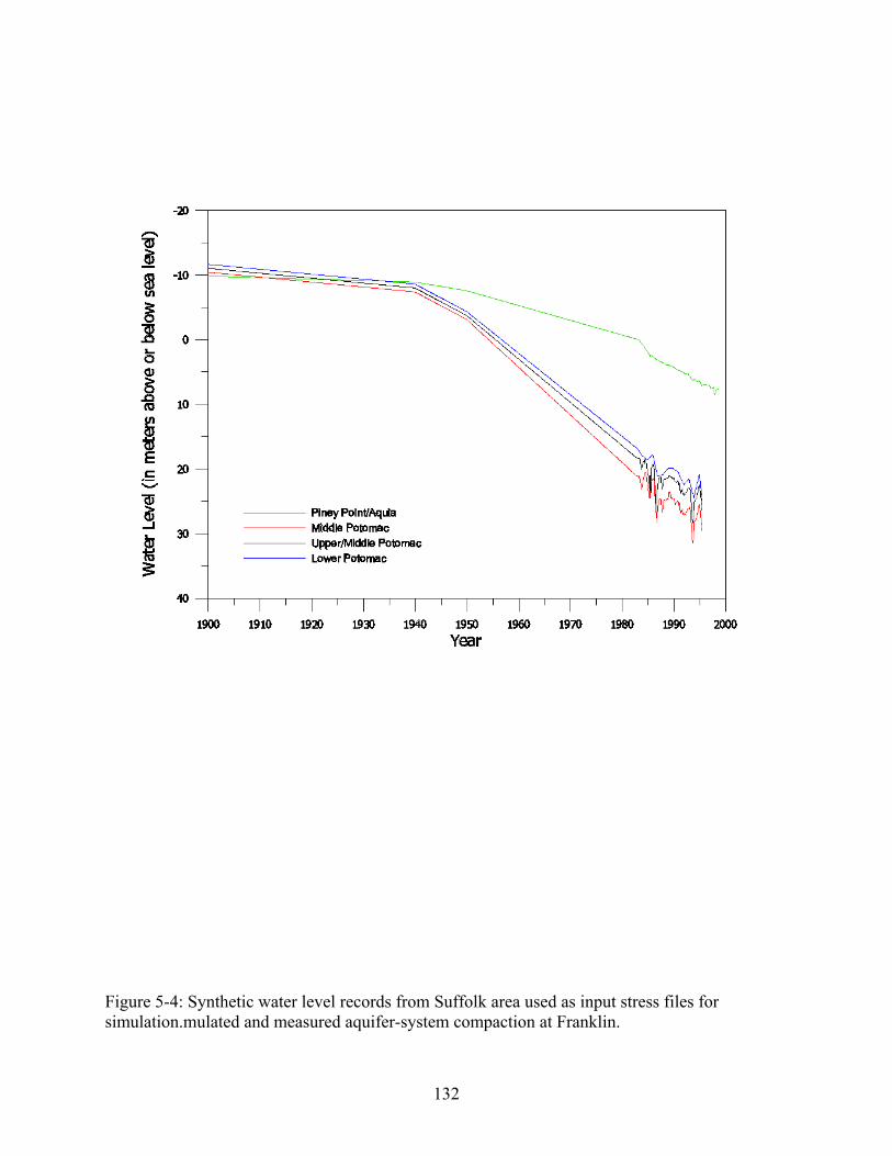
Figure 5-4: Synthetic water level records from Suffolk area used as input stress files for simulation.mulated and measured aquifer-system compaction at Franklin.
132

133

Figure 5-5: Simulated and measured aquifer-system compaction at Franklin.
134

Figure 5-5a: Close-up of simulated and measured aquifer-system compaction at Franklin for period of measured extensometer record.
135

Figure 5-6: Simulated and measured aquifer-system compaction at Suffolk.
136

Figure 5-7: Comparison of simulated compaction at Franklin for fine-grained confining units and aquitards (blue) and coarse-grained aquifer units (red). Total simulated compaction record is green.
137

Figure 5-8: Comparison of simulated compaction at Suffolk for fine-grained confining units and aquitards (blue) and coarse-grained aquifer units (red). Total simulated compaction record is green.
138

VI. LAND SUBSIDENCE AND RELATIVE SEA-LEVEL RISE
The constraints of one-dimensional modeling limit the direct application of the model
results to the locations explicitly simulated, in this case Franklin and Suffolk. The application of
the parameters developed in this one-dimensional simulation to a three-dimensional groundwater
flow model is necessary to accurately predict aquifer-system compaction and the resulting land
subsidence across a large area like the Virginia Coastal Plain. Nonetheless, some general
predictions and calculations can be made in the absence of such a model, given the relative
consistency of the geologic units across the region. It should be noted, however, that the
thickness of these units varies considerably across the Coastal Plain, and this change in thickness
can significantly influence the computation of compaction and subsidence, as the results from
Franklin and Suffolk revealed.
If it is assumed that the modeled value for preconsolidation stress is approximately
correct, then substantial subsidence may have occurred at any location where head decline in the
Potomac aquifer system has exceeded 20 meters from predevelopment conditions. Referring
back to the map of the potentiometric surface for the Middle Potomac aquifer in 1998 (figure
1-2), we can estimate the extent of this stress condition with the aid of geographic information
systems techniques. This relatively crude calculation reveals that the area of eastern Virginia
affected by subsidence resulting from groundwater withdrawals extends from the North Carolina
border to the middle of the Middle Peninsula and from the Chesapeake Bay almost to the Fall
Line (figure 6-1).
Furthermore, observations of changes in the potentiometric surface over several decades
indicate that the regional cone of depression depicted in figure 1-2 is expanding northward (as
populations grow in the counties of Virginia’s Middle Peninsula and Northern Neck) and
eastward (as communities along the Chesapeake Bay begin to pump and treat more brackish
water from the Potomac system in those locations). The result of these changes is that the area
affected by land subsidence is likely to grow, and rates of subsidence might reasonably be
expected to increase in some locations, particularly along the western shore of the Chesapeake
Bay.
Given the small rates of land subsidence observed in eastern Virginia, small increases in
those rates may have relatively insignificant consequences, but any consequences are likely to be
most severe in low-lying coastal areas subject to the effects of rising sea levels. The analysis of
139

sea level rise is extremely complicated and well beyond the scope of this document, but it is
interesting to note that the rate of relative sea level rise (measured from long-term staff gauges)
has been observed to be anomalously high in southeastern Virginia, just a few miles from
Suffolk. In fact, rates of relative sea-level rise at several locations in southeastern Virginia have
been observed to be much higher than the approximately 2 mm/year average for the Atlantic
Coast and elsewhere in the Chesapeake Bay over the period 1950-1993 (http://co-
ops.nos.noaa.gov/seatrnds.html), (figure 6-2). The highest rate of relative sea-level rise in the
region over this period, 4.1 mm/year, was measured at Portsmouth, Virginia. This rate of relative
sea-level rise at Portsmouth is approximately equal to the sum of the measured compaction rate
near Portsmouth and the average rate of sea-level rise along the Atlantic coast.
Land subsidence has been observed to have the most significant cultural and
environmental effects in coastal areas where it magnifies the effects of rising sea levels. Even at
these relatively low rates, land subsidence can have serious effects. For example, reports from
the Virginia Institute of Marine Science (VIMS) have indicated higher than normal rates of
erosion of tidal marshes in this area, with associated habit loss (Carl Hershner, VIMS, oral
communication, 2001). It may be too early to attribute these losses to land subsidence, but
further studies are underway.
As part of the Chesapeake Bay program conducted by the National Oceanic and
Atmospheric Administration (NOAA), a number of long-term global positioning system (GPS)
stations have been established in recent years to monitor land-surface movements in the bay area
(http://www.ngs.noaa.gov/GRD/GPS/Projects/CB/MAP/map.html). These GPS stations are
currently collecting elevation data in order to establish long-term trends, though land-surface
movements of just a few millimeters per year are currently below the resolution of the
instruments. Nonetheless, GPS techniques provide perhaps the best way to monitor land-surface
movements over this region. Concurrently, continued direct measurements of aquifer-system
compaction at the Franklin and Suffolk extensometer sites will enable comparison to land-
surface movements derived from remote sensing techniques, resulting in a better understanding
of the environmental changes resulting from groundwater withdrawals in eastern Virginia,
Maryland and North Carolina.
140

Figure 6-1: Map of estimated area affected by measurable land subsidence due to ground water withdrawals. Shaded are depicts region of greater than 20-meter head decline from predevelopment conditions, which should be associated with land subsidence.
141
R
R
GRFranklin
Suffolk
West Point

Figure 6-2: Mean rates of relative sea level rise (mm/year) in the Chesapeake Bay area from 1950 through 1993.
142
!(
!(
!(
!(
!(
!(
!(
!(
!(
!(
Portsmouth
Hampton Roads
Lewes
Gloucester Point
Solomons Island
DC
Baltimore
Annapolis
LOCATION 1950-1993 (mm/yr)Portsmouth 4.10 Hampton Roads 3.99Gloucester Point 3.40Solomons Island 3.10Annapolis 2.92Lewes 2.57Baltimore 2.26Washington DC 2.20
VII. SUMMARY
Over the past century, large increases in ground-water withdrawals from the confined
aquifers of the Virginia Coastal Plain have resulted in large declines in hydraulic heads and
measurable amounts of subsequent land subsidence. Measurement and simulation of aquifer-
system compaction indicate that the magnitude and rate of compaction and the resulting land
subsidence in this region are small when compared with many other areas experiencing
subsidence. Nonetheless, analyses of extensometer measurements have confirmed that measured
compaction is the result of ground-water withdrawals from the confined aquifers, and
simulations have increased our understanding of the complex relation between measured
hydraulic heads and compaction in this system. Simulation results explain the uneven spatial and
temporal distribution of compaction in the aquifers and confining units of the Coastal Plain. In
addition, simulations have revealed that storage values for the fine-grained units in the Coastal
Plain are larger that previously thought, suggesting that confining-unit storage may substantially
affect ground-water flow in this complex aquifer system. These results are expected to be useful
in ongoing efforts to simulate ground-water flow. Previous flow models of the Virginia Coastal
Plain have not considered the effects of confining-unit storage, which may be important for
accurate calibration of hydraulic heads, particularly for transient simulations. Furthermore,
measurements and simulations of compaction may be useful for predicting and managing land
subsidence in coastal environments.
143

REFERENCES Bates, Robert L., and Jackson, Julia A., 1984, American Geological Institute Dictionary
of Geological Terms. Doubleday Publishing Group, 571 p. Brown, G.A., and Cosner, O.J., 1974, Ground-water conditions in the Franklin area,
Southeastern Virginia: U.S. Geological Survey Hydrologic Investigations Atlas, HA 538.
Bull, W.B., and Poland, J.F., 1974, Land subsidence due to ground-water withdrawal in the Los Banos-Kettleman City Area, California-Part 3, Interrelations of water-level change, change in aquifer-system thickness, and subsidence: U.S. Geological Survey Professional Paper 437-G.
Bull, William B., and Miller, Raymond E., 1975, Land subsidence due to ground-water withdrawal in the Los Banos-Kettleman City Area, California-Part 1, Changes in the hydrologic environment conducive to subsidence: U.S. Geological Society Professional Paper 437-E, 71 p.
Burbey, T.J., 2001, Storage coefficient revisited: Is purely vertical strain a good assumption?: Ground Water 39, no. 3, p. 458-464.
Carpenter, M.C., 1987, Water-level declines, land subsidence, and specific compaction near Apache Junction, south-central Arizona: U.S. Geological Survey Water-Resources Investigations Report 86-4071, 22 p.
Cederstrom, D.J., 1945, Geology and ground-water resources of the Coastal Plain in southeastern Virginia: Virginia Geological Survey Bulletin 63, 484 p.
Cederstrom, D.J., 1957, Geology and ground-water resources of the York-James Peninsula, Virginia: U.S. Geological Survey Water-Supply Paper 1361, 237 p.
Clark, W.B., and Miller, R.L., 1912, The physiography and geology of the Coastal Plain province of Virginia: Virginia Geological Survey Bulletin 4, p. 13-322.
Cooper, H.H., Jr., 1966, The equation of groundwater flow in fixed and deforming coordinates: Journal of Geophysical Research, 71: 4785-90.
Cosner, O.J., 1975, A predictive computer model of the Lower Cretaceous aquifer, Franklin area, Southeastern Virginia: U.S. Geological Survey Water-Resources Investigations Report 51-74, 62 p.
Crank, J., and P. Nicholson, 1947, A practical method for numerical evaluation of solutions of partial differential equations of the heat conduction type: Proc. Camb. Phil. Soc., 43, 50-67.
Davis, G.H., 1977, Potential for land subsidence due to reduction of artesian head in the Atlantic Coastal Plain in Hydraulics in the coastal zone: American Society of Civil Engineers Specialty Conference, College Station, Texas, 10-11 August, p. 152-160.
Davis, G.H., 1987, Land subsidence and sea level rise on the Atlantic Coastal Plain of the United States: Environmental Geology and Water Science, v. 10, no. 2, p. 67-80.
144

Epstein, Victoria J., 1987, Hydrologic and geologic factors affecting land subsidence near Eloy, Arizona: U.S. Geological Survey Water-Resources Investigations Report 87-4143, 28 p.
Erwin, M.L., McFarland, E.R., and Bruce, T.S., 1999, USGS ground-water flow model – an essential tool for managing the water supply of the Virginia Coastal Plain: U.S. Geological Survey Fact Sheet 099-99, 4 p.
Fetter, C.W., 1994, Applied hydrogeology, 3rd ed. Upper Saddle River, New Jersey: Prentice Hall, Inc., 691 p.
Focazio, M.J., and Samsel, T.B., III, 1993, Documentation of geographic-information-system coverages and data-input files used for analysis of the geohydrology of the Virginia Coastal Plain: U.S. Geological Survey Water-Resources Investigations Report 93-4015, 53 p.
Gabysch, R.K., 1984, Case histories of land subsidence due to groundwater withdrawal – Houston-Galveston region, Texas, U.S.A., in Guidebook to studies of land subsidence due to ground-water withdrawal: UNESCO Studies and Report on Hydrology v. 40, 324 p.
Galloway, D.L., Jones, D.R., and Ingebritsen, S.E., 1999, Land subsidence in the United States: U.S. Geological Survey Circular 1182, 175 p.
Gibson, T.G., 1982, Depositional framework and paleoenvironments of Miocene strata from North Carolina to Maryland: p. 1-22 in Miocene of the southeastern United States, Florida Department of Natural Resources, Bureau of Geology Special Publication no. 25, 319 p.
Hamilton, P.A., and Larson, J.D., 1988, Hydrogeology and analysis of the ground-water flow system in the Coastal Plain of Southeastern Virginia: U.S. Geological Survey Water-Resources Investigations Report 87-4240, 175 p.
Hansen, H.J., 1972, A user’s guide for the artesian aquifers of the Maryland Coastal Plain, Part 2 – Aquifer characteristics: Maryland Geological Survey, 123 p.
Hanson, R.T., 1989, Aquifer-system compaction, Tucson basin and Avra Valley, Arizona: U.S. Geological Survey Water-Resources Investigations Report 88-4172, 69 p.
Harsh, J.F., and Lacnziak, R.J., 1990, Conceptualization and analysis of ground-water flow system in the Coastal Plain of Virginia and adjacent parts of Marland and North Carolina: U.S. Geological Survey Professional Paper 1404-F, 100 p.
Heath, R.C., 1983, Groundwater Regions of the United States: U.S. Geological Survey Water-Supply Paper 2242, p. 52-55.
Helm, D.C., 1974, Evaluation of stress-dependent aquitard paramters by simulation of observed compaction from known stress history: Ph.D. dissertation, 175 pp., University of California, Berkeley, 1974.
145

Helm, D.C., 1975, One-dimensional simulation of aquifer-system compaction near Pixley, California, 1. Constant parameters: Water Resources Research, v. 11, no. 3, p. 465-478.
Helm, D.C., 1976a, Estimating parameters of compacting fine-grained interbeds within a confined aquifer system by a one-dimensional simulation of field observations: Proceedings of the International Association of Hydrological Sciences, Anaheim Symposium, December 1976, p. 145-156.
Helm, D.C., 1976b, One-dimensional simulation of aquifer system compaction near Pixley, California - 2. Stress dependent parameters: American Geophysical Union, Water Resources Research, v. 12, no. 3, p. 375-391.
Helm, D.C., 1984, Analysis of sedimentary skeletal deformation in a confined aquifer and the resulting drawdown, in Groundwater Hydraulics, J.S. Rosenshein and G.D. Bennett eds.: American Geophysical Union Water Resources Monograph No. 9, p. 29-82.
Holdahl, Sandford R., and Morrison, Nancy L., 1974, Regional investigations of vertical crustal movements in the U.S., using precise relevelings and mareograph data: Technophysics, 23, p. 373-390.
Holzer, T.L., 1981, Preconsolidation stress of aquifer systems in areas of induced land subsidence: Water Resources Research, v. 17, p. 693-704.
Holzer, T.L., 1984, Ground failure induced by ground-water withdrawal from unconsolidated sediments, in Holzer, T.L., ed., Man-induced land subsidence: Geological Society of America Reviews in Engineering Geology, v. 6, p. 67-105.
Hopkins, H.T., Bower, R.F., Abe, J.M., and Harsh, J.F., 1981, Potentiometric-surface map for the Cretaceous aquifer, Virginia Coastal Plain, 1978: U.S. Geological Survey Water Resources Investigations Open File Report 80-965.
Jacob, C.E., 1940, On the flow of water in an elastic artesian aquifer: Transactions, American Geophysical Union, 21:574-86.
Jacob, C.E., 1950, Flow of ground-water, in Engineering hydraulics, ed. H. Rouse, 321-86. New York: John Wiley.
Keys, Scott W., 1990, Borehole Geophysics Applied to Ground-Water Investigations, Techniques of Water-Resources Investigation of the United States Geological Survey, Book 2, Chapter E2, 150p.
Kull, Thomas K., and Laczniak, Randell J., 1987, Ground-water withdrawals from the confined aquifers in the Coastal Plain of Virginia, 1891-1983: U.S. Geological Survey Water-Resources Investigations Report 87-4049, 37 p.
Laczniak, R.J., and Meng, A.A., 1988, Ground-water resources of the York-James Peninsula of Virginia: U.S. Geological Survey Water-Resources Investigations Report 88-4059, 178 p.
146

Leahy, P.P., and Martin, Mary, 1993, Geohydrology and simulation of ground-water flow in the Northern Atlantic Coastal Plain aquifer system: U.S. Geological Survey Professional Paper 1404-K, 81 p.
Leake, S.A., and Prudic, D.E., 1991, Documentation of a computer program to simulate aquifer-system compaction using the modular finite-difference ground-water flow model: U.S. Geological Survey, Techniques of Water-Resources Investigations Report, Book 6, Chapter A2, 68 p.
Lofgren, B.E., 1968, Analysis of stress causing land subsidence: U.S. Geological Survey Professional Paper 600-B, p. B219-B225.
Lofgren, B.E., 1969, Field measurement of aquifer-system compaction, San Joaquin Valley, California, USA, in Tison, L.J., ed., Land subsidence, v. 1: International Association of Scientific Hydrology, Publication 88, p. 272-284.
McFarland, E. Randolph, 1998, Design, revisions, and considerations for continued use of a ground-water-flow model of the Coastal Plain aquifer system in Virginia: U.S. Geological Survey Water Resources Investigations Report 98-4085, 49 p.
McFarland, E.R., 1999, Hydrogeologic framework and ground-water flow in the Fall Zone of Virginia: U.S. Geological Survey Water-Resources Investigations Report 99-4093, 83 p.
Meng, A.A., and J.F. Harsh, 1988, Hydrogeologic framework of the Virginia Coastal Plain: U.S. Geological Survey Professional Paper 1404-C, 82 p.
Mixon, R.B., Berquist, C.R., Newell, W.L., Johnson, G.H., Powars, D.S., Schindler, J.S., and Rader, E.K., 1989, Geological map and generalized cross sections of the Coastal Plain and adjacent parts of the Piedmont, Virginia: U.S. Geological Survey Miscellaneous Investigations Series Map I-2033, 2 sheets, scale 1:250,000.
Poag, C.W., 1997, The Chesapeake Bay bolide impact – a convulsive event in Atlantic Coastal Plain evolution, in Seagall, M.P., Colquhoun, D.J., and Siron, D., eds., Evolution of the Atlantic Coastal Plain – sedimentology, stratigraphy, and hydrogeology: Sedimentary Geology, v. 108, p. 45-90.
Poag, W.C., Powars, D.S., Poppe, L.J., and Mixon, R.B., 1994, Meteroid mayhem in Ole Virginny – source of the North American tektite strewn field: Geology, v. 22, p. 691-694.
Poland, J.F., and Davis, G.H., 1969, Land subsidence due to withdrawal of fluids, in Varnes, D.J., and Kiersch, George, eds., Reviews in Engineering Geology, v. 2: Boulder, Colorado, Geological Society of America, p. 187-269.
Poland, J.F., ed., 1984, Guidebook to studies of land subsidence due to ground-water withdrawal: UNESCO Studies and Report on Hydrology v. 40, 324 p.
Poland, J.F., Lofgren, B.E., Ireland, R.L., and Pugh, R.G., 1975, Land subsidence in the San Joaquin Valley, California, as of 1972: U.S. Geological Survey Professional Paper 437-H, 78 p.
147
Poland, J.F., Lofgren, B.E., and Riley, F.S., 1972, Glossary of selected terms useful in studies of the mechanics of aquifer systems and land subsidence due to fluid withdrawal: U.S. Geological Survey Water-Supply Paper 2025, 9 p.
Powars, D.S., 2000, The effects of the Chesapeake Bay impact crater on the geologic framework and the correlation of hydrogeologic units of southeastern Virginia, south of the James River: U.S. Geological Survey Professional Paper 1622, 53 p.
Powars, D.S., and Bruce, T.S., 1999, The effects of the Chesapeake Bay impact crater on the geological framework and correlation of hydrogeologic units of the lower York-James Peninsula, Virginia: U.S. Geological Survey Professional Paper 1612, 82 p., 7 pl.
Reinhardt, Juergen, Christopher, R.A., and Owens, J.P., 1980, Lower Cretaceous stratigraphy of the core, in Geology of the Oak Grove Core: Virginia Division of Mineral Resources Publication 20, part 3, p. 31-52.
Remson, I., Homberger, G.M., and Molz, F.J., 1971, Numerical methods in subsurface hydrology: New York, John Wiley and Sons, Inc., 389 p.
Richardson, D.L., Laczniak, R.J., and Hamilton, P.A., 1988, Evaluation of Municipal Withdrawals from the Confined Aquifers of Southeastern Virginia: U.S. Geological Survey Open-File Report 88-723, 50 p.
Riley, F.S., 1969, Analysis of borehole extensometer data from central California, in Tison, L.J., Land Subsidence: International Association of Hydrological Sciences Publication 89, v. 2, p. 423-431.
Riley, F.S., 1984, Developments in borehole extensometry, in Johnson, A.I., Carbognin, L., and Ubertini, L., eds., Land Subsidence: International Association of Hydrological Sciences Publication 151, p. 169-186.
Sanford, Samuel, 1913, The underground water resources of the Coastal Plain province of Virginia: Virginia Geological Survey Bulletin 5, 361 p.
Scott, R.F., 1963, Principles of soil mechanics: Palo alto, Addison-Wesley, 550 p. Sneed, M., and Galloway, D.L., 2000, Aquifer-system compaction and land subsidence:
measurements, analyses, and simulations – the Holly site, Edwards Air Force Base, Antelope Valley, California: U.S. Geological Survey Water-Resources Investigations Report 00-4015, 65 p.
Terzaghi, K., 1925, Principles of soil mechanics, IV – Settlement and consolidation of clay: Engineering News-Record, 95(3), p. 874-878.
Terzaghi, Karl, and Peck, R.B., 1948, Soil mechanics in engineering practice: New York, John Wiley and Sons, Inc., 566 p.
Tolman, C.F., and Poland, J.F., 1940, Ground-water infiltration, and ground-surface recession in Santa Clara Valley, Santa Clara County, California: Transactions American Geophysical Union, v. 21, p. 23-24.
Verruijt, A., 1968, Elastic storage of aquifers: in Flow through porous media, R.J.M De Wiest ed., New York, Academic Press, p. 331-376.
148

White, R.K., and Powell, E.D., 1996, Water resources data – Virginia – water year 1996; volume 2 – ground-water level and ground-water quality records: U.S. Geological Survey Water-Data Report VA-96-2, 363 p.
Wolff, R.G., 1970, Relationship between horizontal strain near a well and reverse water level fluctuation: Water Resources Research, v. 6, no. 6, p. 1721-1728.
149

JASON PHILIP POPE
U.S. Geological Survey, Water Resources Discipline 1730 E. Parham Road, Richmond, Virginia 23228; (804) 261-2627
e-mail: [email protected] EDUCATION: Virginia Polytechnic Institute and State University M.S. in Geological Sciences (Hydrogeosciences), June 2002 Thesis title: Characterization and Modeling of Land Subsidence due to Groundwater
Withdrawals from the Confined Aquifers of the Virginia Coastal Plain University of North Carolina at Asheville B.S. in Environmental Studies (Waste Management), May 1994 Research title: Phosphorus Retention in a High-Elevation Southeastern Reservoir System
NATURAL SCIENCES WORK EXPERIENCE: U.S. Geological Survey, Water Resources Discipline, Virginia District Hydrologist. June 2001 to Present.
Currently working as part of a team on a regional-scale groundwater flow model of the Virginia Coastal Plain. Duties include quantifying groundwater withdrawals in eastern Virginia, evaluating water levels in regional aquifers, assisting with re-interpretation of the regional hydrogeologic framework, and assisting with the production and evaluation of the groundwater model. Responsible for managing all geologic and hydrologic data for the project using geographic information systems (GIS) techniques.
Environmental Systems and Technologies, Inc.
Assistant Scientist II. June 2000 to October 2000. Duties focused on predictive modeling of groundwater flow and transport of contaminants, particularly those associated with hydrocarbon leaks and spills. Modeled subsurface migration of non-aqueous-phase liquids such as gasoline, as well as transport of the associated dissolved constituents. Other duties included management and statistical analysis of data from a variety of contaminated sites, interpretation of drilling logs, and preparation of reports and presentations. Position was terminated due to corporate restructuring.
Virginia Tech Department of Geological Sciences
Graduate Teaching Assistant. August 1997 to July 1999; January to May, 2001. Taught Physical Geology Laboratory and Resources Geology Laboratory Graduate Research Assistant. August 1999 to May 2000.
Worked on the measurement and modeling of land subsidence in eastern Virginia.
150

University of Vermont Geology Department Research Assistant. September to December, 1994. Worked with interdisciplinary team monitoring and analyzing phosphorus transport and cycling in the Lake Champlain basin. Collected and processed field samples of river-bottom sediments and analyzed total and available phosphorus content of size fractions. UNC Asheville Environmental Quality Institute Lab Technician, Analytical Chemist, and Research Assistant. May 1991 to June 1994. Performed environmental research as part of a small team under the direction of Dr. Richard Maas of the Environmental Studies Program and in conjunction with several environmental organizations. Duties included analysis of soil and water samples in an EPA-certified laboratory, performance of field water-quality and hydrology projects, and extensive library research and data analysis. Assisted with the coordination of several large research projects and co-authored a variety of technical reports on subjects ranging from water quality of area streams to lead leaching from brass faucet fixtures. Proficient in the use of AA Spectrophotometer for analysis of trace metals, as well as a variety of other analytical methods. Also worked as a consultant on various projects since 1994. Metropolitan Sewerage District of Asheville, NC Internship: Assistant Wastewater Treatment Plant Operator. Summer 1992. Learned and performed operational duties as part of a small team at a municipal waste water treatment facility. Also worked with pre-treatment monitoring program.
STUDENT SERVICES WORK EXPERIENCE:
Department of Housing and Residence Life, UNCA, Asheville, NC Resident Director. Full-time: July ‘96 to August. ’97. Part-time: May ‘95 to June ‘96.
Responsible for operation and live-in supervision of a 300-bed co-educational campus residence hall facility. Duties included assisting with development and supervision of 45 student Resident Assistants; directly supervising 15 student Night Assistants; planning educational and social activities; meeting with students regarding disciplinary matters; mediating disputes among students; and performing other related tasks.
Department of Student Activities, UNCA, Asheville, NC Student Activities Technical Assistant. Part-time: August ‘95 to May ‘96. Performed a variety of duties associated with daily operation of university student center,
including special event planning and support. Keewaydin Foundation, Salisbury, VT Staffman and Trip Leader. Summers of ‘94, ‘97, ‘98.
Served as summer live-in staff member at traditional boys' summer camp focused on wilderness trips and canoeing. Primarily supervised boys between the ages of 12 and 14 years in a variety of recreational activities. Led and coordinated wilderness hiking and canoeing trips.
151

UNCA Dept. of Housing and Residence Life, Asheville, NC Resident Assistant, 1989-1991 and Head Resident Assistant, 1991-1992. Provided leadership, assistance and support to members of the campus residential community. Duties included familiarizing residents with campus resources; mediating disputes; developing and implementing campus educational, recreational and social programs; interpreting and enforcing residence hall regulations; assisting with residence hall security; and responding to emergency situations.
PROFESSIONAL ACTIVITIES: Presentation at USGS Land Subsidence Interest Group Meeting, Fall 2001. Presentation at Virginia Water Research Conference, Fall 1999. Presentation at Geological Society of America Annual Meeting, Fall 1999. Served on Organizational Committee for the Virginia Tech Geological Sciences
Student Research Symposium, 1998-1999. Served on Virginia Tech Geological Sciences seminar committee, 1997-1998.
PROFESSIONAL AFFILIATIONS:
Sigma Xi, National Scientific Research Society; Associate Member National Ground Water Association
RESEARCH IN ENVIRONMENTAL SCIENCES:
Publications:
Pope, J.P., and T.J. Burbey, 2002, “Characterization and Modeling of Land Subsidence due to Ground-Water Withdrawals from the Confined Aquifers of the Virginia Coastal Plain.” Proceedings of the 2001 USGS Land Subsidence Interest Group Meeting, U.S. Geological Survey Open File Report, In Press. Patch, S.C., R.P. Maas, J.P. Pope, 1998. “Lead Leaching from Faucet Fixtures under Residential Conditions.” Journal of Environmental Health, Vol. 61, No. 3 (1998): 18-21.
Maas, R.P., S.C. Patch, J.P. Pope, L. Thornton. 1998. “Lead-Leaching Characteristics of Submersible Residential Water Pumps.” Journal of Environmental Health. Vol. 60, No. 6 (1998): 8-13.
Technical Reports:
Maas, R.P., S.C. Patch, R.L. Winfield, J.P. Pope, D.M. Morgan. “Field-Based Corrosion Control and Monitoring Strategies for Meeting the Lead and Copper Rule Action Levels.” UNC Asheville Environmental Quality Institute Technical Report #94-008. 1994.
Maas, R.P., S.C. Patch, R.L. Winfield, J.P. Pope, D.M. Morgan. “Lead Leaching from New Submersible Well Pumps under Field Usage Conditions.” UNC Asheville Environmental Quality Institute Technical Report #94-007. 1994.
152

Maas, R.P., S.C. Patch, K.E. Jordan, D.J. Kucken, J.P. Pope. “Water Quality of Buncombe County Streams: Year Four Results of the Volunteer Water Information Network.” UNCA Environmental Quality Institute Technical Report #94-006. 1994. Maas, R.P., S.C. Patch, R.L. Winfield, J.P. Pope, D.M. Morgan. “Rinsate Contributions to Adjusted Faucet Fixture Lead Leachate Concentrations.” UNC Asheville Environmental Quality Institute Technical Report #94-005. 1994.
Maas, R.P., S.C. Patch, W.A. Barrett, J.P. Pope. “Initial Lead Leaching Characteristics of Submersible Pumps Used in Residential Wells.” UNC Asheville Environmental Quality Institute Technical Report #94-003. 1994
Maas, R.P., S.C. Patch, J.P. Pope, E.E. Rainey. “The Effects of Acidity, Pre-Cleaning and Surface Coating on Lead Leaching from Standard Leaded-Brass Water Meters.” UNC Asheville Environmental Quality Institute Technical Report #94-002. 1994.
Maas, R.P., S.C. Patch, G.M. Brown, J.P. Pope. “A Statistical Analysis of the Relationship between Public Water Supply Characteristics and At-The-Tap Lead and Copper Levels.” UNC Asheville Environmental Quality Institute Technical Report #94-001. 1994.
Maas, R.P., S.C. Patch, J.P. Pope, D.M. Morgan. “Contribution of Faucet Fixtures to Residential Tap Water Contamination in California.” UNC Asheville Environmental Quality Institute Technical Report #93-007. 1993.
Maas, R.P., D.J. Kucken, J.P. Pope. “A Water Quality Survey of Lake Sequoyah and Mirror Lake, Highlands, NC. UNC Asheville Environmental Quality Institute Technical Report #92-006. 1992.
Pope, J. P., and R. P. Maas. “Phosphorus Retention in a High-Elevation Southeastern Reservoir System.” Oral Presentation at the Sixth National Conference on Undergraduate Research, Minneapolis, Minnesota, 1992.
Note: All EQI technical reports are available from the Environmental Quality Institute, UNCA, Asheville, NC 28804.
153

REFERENCES:
Thomas J. Burbey, Ph.D. M.S. Thesis Advisor
Assistant Professor of Hydrogeosciences Department of Geological Sciences
Virginia Polytechnic Institute and State University Blacksburg, Virginia 24061
(540) 231-6696 e-mail: [email protected]
Ward Staubitz Virginia District Chief
USGS Water Resources Division 1730 E. Parham Road, Richmond, Virginia 28804
(804) 261-2600 e-mail: [email protected]
Richard P. Maas, Ph.D. Undergraduate Advisor
Chair, Environmental Studies Program Associate Professor of Environmental Studies
UNC Asheville Asheville, North Carolina 28804
(704) 251-6366 e-mail: [email protected]
Steven C. Patch, Ph.D. Director, Environmental Quality Institute
Professor of Mathematics UNC Asheville
Asheville, North Carolina 28804 (704) 232-5194
e-mail: [email protected]
Peter Williams Director of Housing and Residence Life
UNC Asheville Asheville, North Carolina 28804
e-mail: [email protected]
154


