
1
Choice Experiments to Assess Farmers' Willingness to Participate in a Water
Quality Trading Market
Jeffrey M. Peterson John A. Fox
John C. Leatherman Craig M. Smith
Kansas State University
May 31, 2007
Contact: Jeff Peterson, Associate Professor Department of Agricultural Economics 216 Waters Hall Kansas State University Manhattan, KS 66506 USA [email protected] 785.532.4487
Selected paper prepared for presentation at the American Agricultural Economics Association Annual Meeting, Portland, Oregon, July 29-August 1, 2007. Copyright 2007 by Jeffrey M. Peterson, John A. Fox, John C. Leatherman, and Craig M. Smith. All rights reserved. Readers may make verbatim copies of this document for non-commercial purposes by any means, provided that this copyright notice appears on all such copies. _________________________ Peterson is associate professor, Fox and Leatherman are professors, and Smith is a watershed economist, all in the Department of Agricultural Economics, Kansas State University, Manhattan, Kansas. The authors are grateful to Kevin Dhuyvetter, Terry Kastens, Jayson Lusk, and John Bernard for helpful comments and suggestions. We also thank Adriana Chacon and Pedro Garay for their able research assistance.

2
Abstract
Interest has grown in Water Quality Trading (WQT) as a means to achieve water quality goals,
with more than 70 such programs now in operation in the United States. Substantial evidence
exists that nonpoint sources can reduce nutrient loading at a much lower cost than point sources,
implying the existence of gains from trade. Despite the potential gains, however, the most
commonly noted feature of existing WQT markets is low trading volume, with many markets
resulting in zero trades. This paper evaluates one explanation for the lack of participation from
agricultural nonpoint sources. We test for and quantify the “intangible costs” that may deter
farmers from trading even if the monetary benefits from doing so outweigh the observable out-
of-pocket costs. We do so by designing and implementing a series of choice experiments to elicit
WQT trading behavior of Great Plains crop producers in different situations. Attributes of the
choice experiment included market rules and features (e.g., application time and effort, penalties
for violations, means of monitoring compliance) that may affect farmers’ willingness to trade.
The choice experiments were conducted with a total of 135 producers at four locations in the
state of Kansas between August 2006 and January 2007. A Random Parameters Logit model is
appropriate to analyze the resulting data, revealing diversity in the way that the attributes affect
farmers’ choices.

3
Choice Experiments to Assess Farmers' Willingness to Participate in a Water Quality Trading Market
Water Quality Trading (WQT) has received increased attention as a means to achieve water
quality goals. Several such trading programs have been adopted in several states throughout the
nation, with more than 70 programs now in operation (Breetz et al., 2004). In principle, such
programs could be applied to any water-borne pollutant and allow trading among point sources,
among nonpoint sources, or between point and nonpoint sources (the latter is known as ‘point-
nonpoint trading’). Most of the existing programs are designed with point-nonpoint trading to
limit nutrient loading: point sources are allowed to meet their nutrient emission limits by
purchasing water quality credits from agricultural producers in the surrounding watershed. These
producers are then obligated to implement a best management practice (BMP) that reduces
expected nutrient loading by an amount commensurate with the number of credits sold.
Substantial evidence exists that nonpoint sources can reduce nutrient loading at a much
lower cost than point source polluters in many watersheds. This suggests that a well functioning
WQT program would be a more cost-effective strategy for meeting total maximum daily load
requirements than regulating point source polluters alone (Faeth, 2000). The potential for
pollution trading to lower control costs has already been realized in the active air quality trading
markets (NCEE, 2001).
Despite the potential gains from WQT, perhaps the most commonly noted feature of
existing programs is low trading volume; none of the programs have had extensive trading
activity and many have had no trading at all (Hoag and Hughes-Popp, 1997). Our particular
interest in this paper is the participation of nonpoint sources, almost always agricultural crop
producers in existing programs. The reluctance of farmers to participate in WQT reflects a

4
broader reluctance to adopt environmental practices in exchange for monetary payments (e.g.,
Cooper and Keim 1996).
Evidently, farmers perceive some intangible costs of participating in WQT markets that
are not offset by the monetary gains from trading. These costs may include the disutility of the
managerial effort required to maintain BMPs, and/or a distaste for the WQT market procedures
and rules. For example, farmers may object to the intrusiveness of being inspected or monitored
to ensure their BMP is in place, or find the process of signing up for the program to be too
onerous.
Although the existence of intangible costs is apparent from empirical evidence, the
factors giving rise to these costs are not well understood. The objective of this paper is to
quantify the impact of different institutional factors on farmer’s stated behavior in a WQT
market. In particular, we wish to determine the importance – relative to monetary trading income
– of various WQT market attributes on farmers’ willingness to participate in such a market. The
magnitude of these factors will provide information about how to design a program to encourage
participation and, more broadly, will identify the situations where a WQT market is feasible
given that certain rules are necessary.
The method of choice experiments is well suited to our research question. Choice
experiments were originally developed in the marketing literature in order to determine the
implicit market value of various product attributes. Subjects in these experiments make a choice
from a side-by-side comparison of 3 or more products, which vary by different attributes
including price. The choice data is then analyzed using discrete choice regression models, such
as conditional logit, to estimate the effect of each attribute on the probability that the consumer
chooses the product. This method has been widely adopted by environmental economists

5
studying choice behavior related to environmental quality, such as selection of recreation sites
(e.g., Adamowicz et al., 1997) and housing location (e.g., Earnhart, 2001). Economists studying
agricultural markets have also applied the method to understand the attributes of food products
influencing consumers’ shopping choices (e.g., Fox et al., 2002).
This paper describes a set of choice experiments designed to elicit WQT trading behavior
of Great Plains crop producers in different situations. In our case, the attributes to be varied
across choices are the features of trading, such as the effort required for signup and the
monitoring the farmer would need to undergo. Choice experiments were conduced in person with
producers at events in different locations in Kansas from August 2006 through January 2007.
Experimental Design
The purpose of our experiments is to identify market rules and attributes that influence farmers’
willingness to participate in a point-nonpoint WQT market. After reviewing the operations of
existing programs and consulting with Extension personnel and a small group of farmers in
Kansas, we identified four market attributes that are likely to affect participation: (1) application
time and effort, (2) the monitoring method, (3) penalties for violations, and (4) the BMP to be
adopted. Embedded within the definition of BMPs is another key attribute: the degree of
flexibility a farmer would have in fulfilling his trading obligations. As noted above, the price of
credits is an additional explicit attribute, which will ultimately allow us to compute the implicit
values of the other four. These attributes are listed in Table 1 and are described in more detail
below.
By designing our experiments with different levels of our five attributes, we generate a
dataset that allows us to test whether the institutional attributes affect trading choices, and if so,

6
the magnitude of these impacts relative to price. Farmers were asked to choose among different
opportunities to trade, which varied across the five attributes. Such choice scenarios would arise
in an actual trading program, for example, if a WQT program were established in some region
that allowed buyers to spell out the terms of the trading contract. Different buyers would then
develop different contracts suiting their needs, giving rise to a range of trading opportunities for
farmers. In the choice experiment method, the attributes are varied systematically based on
experimental design principles, so that the resulting dataset maximizes statistical efficiency. In
what follows, we describe the attributes we vary in our choice experiments and then explain the
procedures we followed to design our choice sets.
Design Attributes
This section describes each of the attributes varied in our experiments and rationale for the levels
we selected (Table 1). As noted above, trading opportunities are defined as different
combinations of these attribute levels. A sample choice scenario presented to farmers is in Figure
1. Each scenario asks farmers to choose one of two trading opportunities, labeled Option A and
Option B, or else choose Option C - “do not enroll.” To facilitate comparison, all trading
opportunities were assumed to be for a 10-year contract on a 100-acre field.
The first attribute in the choice experiment is Application Time. This refers to the amount
of time a potential seller would have to spend to establish his eligibility to enter into a WQT
contract. This time would be expended on such activities as meeting with the staff of the entity
managing the market, compiling data on the field to be enrolled, and filling out paperwork.
Application Time would vary depending on the complexity of the program and the desires of the

7
buyer in the contract. We set this attribute to vary from 4 to 40 hours to enroll a 100-acre field, a
range we assumed was large enough to capture a wide range of contract complexity.
The Monitoring Method has two categorical levels. If Monitoring Method = Annual
Verification, then farmers entering into a contract would be visited at an unannounced time each
year to ensure they are meeting the terms of the contract. The field where the contracted BMP is
to be installed would be inspected to verify that the practice is being implemented and
maintained as agreed. If Monitoring Method = Spot Check, then the farmer would be visited with
a 10% probability each year, implying that one visit would occur during an average 10-year
contract period. If visited, the type of inspection would be the same as with Annual Verification.
These two possibilities reflect varying levels of “intrusiveness” the seller must be willing to
accept.
The Penalty is a one-time fine to be paid if the seller is found in violation of the contract.
Levels of this attribute range from $50/acre to $500/acre, a sufficiently wide variation to ensure
that farmers would not find it rational to “plan on cheating” and paying the fine when caught. For
example, under the Spot Check system of monitoring, the upper end of this range produces an
expected penalty from cheating of $50/acre/year. This exceeds the maximum revenue that could
be earned from entering into a contract ($25/acre/year - see below), which is also the maximum
possible gain from cheating on a contract.
The BMP is the fourth attribute, which takes on four categorical levels indicating four
distinct BMPs. The four BMPs vary along two dimensions. The first dimension is the type of
practice – the farmer must either install a filter strip or implement no-till. The second dimension
is the level of flexibility the farmer would have in meeting his contract obligations. In the case of
filter strips the more flexible option would allow farmers to hay and or graze the filter-designated

8
area. For no-till, flexibility comes in the form frequency of use – “rotational no-till” allows for
some other tillage practice in 5 out of the 10 years under contract. We designed our scenarios so
that Option A was always of the filter strip variety and Option B was always of the No-till
variety. This reduces the number of degrees of freedom in our experimental design, by
effectively reducing this four-level attribute to a two-level attribute.
The BMPs will be a significant determinant of farmers’ choice if they value flexibility, or
if they perceive differences in implementation costs. One complication in comparing the BMPs
is that filter strips involve up-front installation costs: the land for the filter strip must be tilled,
leveled, and seeded to grass in the first year. On the other hand, KSU Extension crop budgets
indicate an expected cost of zero for a typical Kansas farmer to implement no-till. To make this
comparison more straightforward for respondents, they were told that the installation costs of
filter strips would be covered from “an outside source.” This is not unrealistic, as cost share
funds from both state and federal programs are available to pay for installing buffer strips
statewide.
Another reason we removed the installation costs was to focus the respondent’s attention
on comparing the ongoing managerial costs of the practices. To clarify the managerial costs of
each of these practices, farmers were given specific definitions of the practices along with a list
of maintenance responsibilities. “100% No-till,” for example, was defined as the tillage practice
where the only equipment that breaks the soil surface is a planter, and this occurs at most once
annually. For filter strips, the maintenance requirements were to regularly check for and repair
any gullies that develop, to avoid using the filter strip as a roadway, and to avoid broadcast
application of chemicals or manure in the filter strip area.
9
The final attribute is trading revenue, or the price per credit multiplied by the number of
credits generated from the BMP. We varied trading revenue from $3/acre/year to $25/acre/year,
following the range used by Cooper and Keim (1996) and Cooper (1997). Each BMP was
assumed to generate a fixed number of credits (Table 2), and the price per credit was calculated
in each scenario so that price times credits equaled the specified revenue level. For example, in
Option A of the scenario shown in figure 1, our experimental design called for a revenue of
$15/acre/year and a BMP of Filter Strip (with haying/grazing), a practice which would generate
6 credits/acre (Table 2).The price per credit was then calculated as $15/6 = $2.50. As described
below, we generated 32 different choice sets encompassing 64 distinct trading choices. Across
all 64 choices, the variation in credits (see table 2) combined with the variation in revenue ($3-
$25) produced a variation in the price per credit of $0.25 to $5.00.
Design Procedures
As noted above, our experimental subjects were to respond to choice sets, each of which contains
two trading opportunities with five attributes. Thus there are a total of ten attributes to be varied
across choice sets. Our experimental design problem is to construct a collection of choice sets by
systematically varying these 10 factors. 6 of these factors have 4 levels and the remaining 4 have
2 levels, implying that a complete factorial spanning all possible combinations these factors
would require 65,536 distinct choice sets – obviously a prohibitive number of scenarios to
present to respondents.
We used the SAS %MktRuns macro (Kuhfeld, 2005) to identify the minimum number of
choice sets in an orthogonal main effects design. An orthogonal main effects design is a small
sample of all combinations in the full factorial, where the chosen combinations exhibit a zero

10
correlation among the attributes. The smallest orthogonal main effects design contains 32 choice
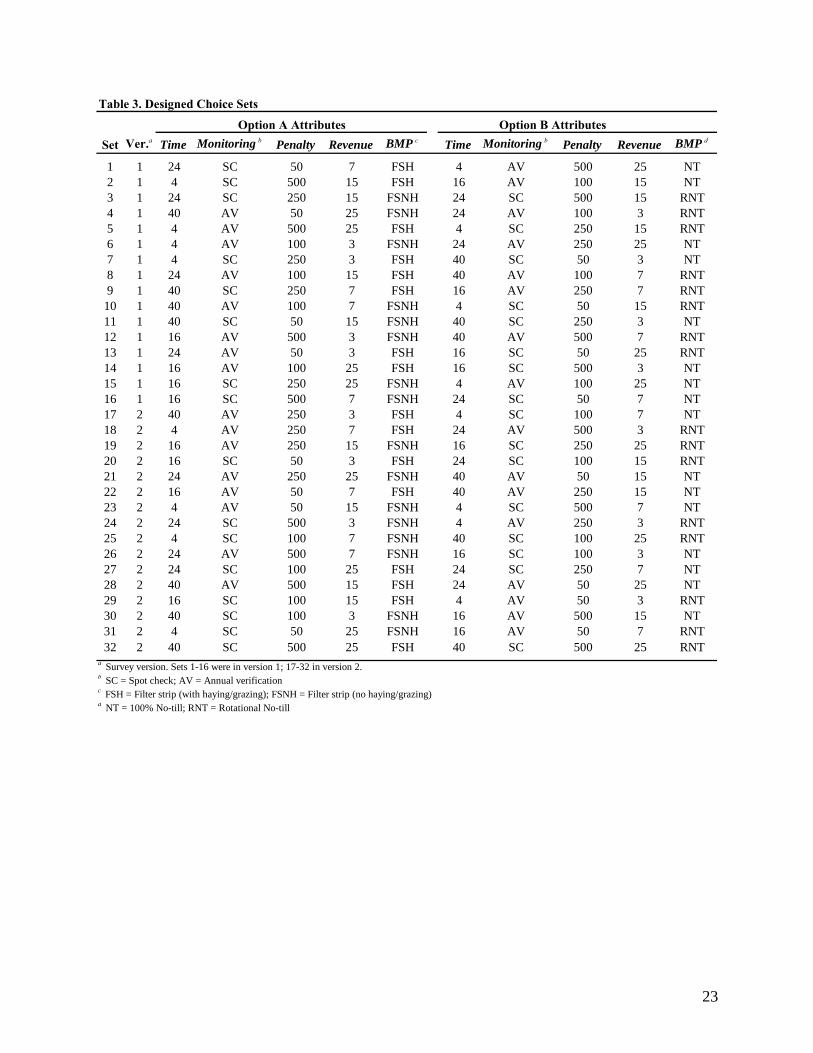
sets, and such a design was constructed using the SAS %MktEx macro (Kuhfeld, 2005). The
choice sets were then blocked into two sets of 16, so that our choice experiment came in two
versions. The choice sets in our design are shown in table 3.
Data
Collection Procedures
Our choice experiments were conducted in person with farmers at different producer-oriented
conferences in Kansas. A total of 135 subjects completed the experiment at four different events
between August 2006 and January 2007 (Table 4). The Risk and Profit Conference is an annual
event hosted by the Agricultural Economics Department at KSU, drawing participants from all
around the state. The second event was a statewide Farm Bureau conference, in January 2007 in
Wichita. The Agricultural Profitability Conferences are run by KSU Extension economists at
various locations around the state in winter months, and mainly draw regional audiences (Colby
and Smith Center are in western and central Kansas, respectively). The Farm Bureau conference
is also a statewide event. The events were chosen in part to ensure a representative geographic
distribution of farmers across the state.
Our data collection procedures at all these events were as follows. First, experimental
subjects were recruited via a pre-registration mailing and an announcement at the opening
conference session. The choice experiment itself was conducted during a 1-hour session,
typically scheduled as a parallel session in the conference program. During this session, subjects
wewre first shown a brief presentation on the concept of Water Quality Trading, followed by
instructions to complete the choice experiments.

11
The instructions include much the same information as in the Design Attributes section
above. A hypothetical situation was first described, in which subjects are asked to imagine that a
WQT program had been developed in their region with different buyers giving them different
types of opportunities to sell credits. The opportunities varied along five dimensions (the
attributes in table 1). These attributes and their various levels were then explained. BMPs were
explained in more detail than the other attributes to ensure that the producers understood what
their contract responsibilities would be under each. Finally, the respondents were shown an
example choice set to give them practice in completing the experiment.
After allowing for clarification questions, the subjects then filled out a booklet with 16
choice sets. A printed copy of the background and instruction slides were also provided to
subjects for their reference, and the instructions were also summarized at the beginning of the
booklet. Each choice set in this booklet is followed by an open-ended question asking, “Why did
you make this choice?” As explained in more detail below, these qualitative responses were
helpful in choosing our econometric specification. After completing the booklet each subject
completed a questionnaire eliciting information on his/her farm operation, his/her attitudes
toward water quality issues and policies, and demographic data. Copies of all materials used in
these sessions are available from the authors.
After the instruments have been completed, each subject was paid an honorarium of $50
in cash. This is announced in the pre-registration mailing and at the opening conference session
to encourage participation. Our data collection procedures and instruments were pre-tested with a
small group (12) of producers from the Great Plains.

12
Questionnaire Data
Summary statistics from the questionnaire responses (n=135) are in Table 5. The average farmer
in this sample owns 824 acres of cropland and rents 773 acres, for an average farm size of 1,597
acres. However, the distribution of size is skewed, with a few very large operations; the
maximum owned acres is 6,000 and the maximum rented acres is 10,000. These statistics are
reflective of the overall distribution of farm sizes in Kansas, which has a few large farms at the
upper tail of the distribution. Based on the 2002 Census of Agriculture, about 10% of all farm
operations in Kansas exceed 2,000 acres (NASS).
Many of the producers in the sample currently use one or more BMPs. The most popular
BMP is minimum tillage, used by 55% of respondents, while the least popular on the list was
filter strips, with only 19% of respondents using this practice. Notwithstanding farmers’
willingness to adopt BMPs, there is a persistent gap between their awareness of conservation
programs and their participation in them. For example, 97% respondents are aware of the
Conservation Reserve Program, but only 45% have participated in it. The gap is particularly
stark for the Environmental Quality Incentives Program (EQIP), which has an awareness rate of
about 80% but a participation rate of 31%. Similarly large gaps are present for the Conservation
Security Program and the Kansas Buffer Initiative. Because these programs offer incentives that
match and in some cases outweigh the monetary expenses of installing BMPs, the observed
participation gap is consistent with the presence of intangible costs as reviewed above.
In terms of perceptions, farmers agree with the sentiment that water quality needs to be
protected and that BMPs help reduce nutrient and sediment runoff. However, the average
respondent was neutral on whether Kansas water supplies are polluted. The average response
was also neutral on the statements that “Mandating BMP installation and management is unfair

13
to producers,” and that “Environmental legislation is often unfair to producers.” Two perception
questions were included to test a commonly state hypothesis in the literature (e.g., King and
Kuch, 2003) that farmers are reluctant to participate in WQT because they fear future regulation.
The average respondent in our sample only slightly agreed with the statements that “A farmer
who participates in a WQT market is more likely to be regulated in the future, compared to
nonparticipants,” and that “If WQT markets emerge and are successful, future government
regulations on agriculture will be more stringent than otherwise.” However, neither average is
statistically different from zero. Thus, we find little evidence that such concerns prevent farmers
from participating, at least explicitly. Finally, the experiment itself appeared to increase subjects’
knowledge of WQT, with the self-assessed level of knowledge increasing, on average, about 1.3
points on a 5-point scale. The distribution of scores was also significantly tighter following the
experiment.
The demographic data from our sample suggest it is fairly representative of the larger
farm population. The average age of producers in our sample is 41.5 and is not statistically
different from the population average of 56 based on the 2002 Census of Agriculture (NASS).
About 81% of our respondents were male, compared to 91% of primary farm operators in
Kansas, but again the difference is not statistically significant. The average producer has 15 years
of formal education, or about 3 years beyond high school, and about 58% of respondents farm as
their primary occupation.

14
Choice Data
Turning now to the choice experiments, we recorded the choice made in 16 distinct scenarios by
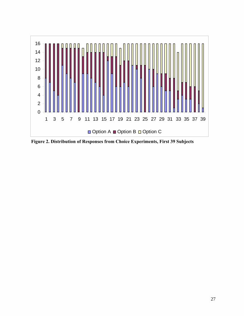
135 subjects, producing a dataset with 2,147 usable observations.1 To give a sense of the choices
the subjects made, Figure 2 shows the composition of these data across the 3 choices (options A,
B, C) for the first 39 subjects in our dataset. Subjects in the figure are sorted by their frequency
of choosing option C, the “do not participate” alternative. All 39 subjects chose to participate in
the program (i.e., selecting either option A or B) in at least one scenario, and four subjects chose
to participate in all 16 scenarios.
Participation was not dominated by either filter strip (option A) or no-till (option B)
contracts. In scenarios where they participated, all but six subjects stated a willingness to choose
either option, switching between the two as the non-BMP attributes (application time,
monitoring, etc.) varied. In particular, only three subjects (#9, #25, #37) never chose option A
and three additional subjects (#22, #26, #39) never chose B. Across the 620 choice sets in this
sub-sample, the distribution across the three choices were: A – 235 (38%), B – 205 (33%), and
C – 180 (29%).
On the whole, our dataset is quite balanced dataset across the three alternatives. This
property is one way of validating the ranges of the non-BMP attributes: these attributes were
varied widely enough to entice participation in both types of BMP contracts, but also led to
nonparticipation in some cases. Balance is also important because we will employ a discrete
choice econometric model for analysis – a model family known to be unstable and to predict
poorly if the dataset is unbalanced across choices.
1 Across all 135×16 = 2,160 choice sets presented to subjects, 13 choice responses were either missing or unreadable.

15
Model
Various discrete choice econometric methods have been used to analyze choice experiment data,
but all these methods are motivated by the random utility model. Suppose that on occasion t,
individual i must chose one of several alternatives indexed by j. Let Uijt denote the utility
enjoyed by individual i if he chooses alternative j on occasion t. The random utility model posits
that Uijt can be partitioned into two additive components:
Uijt = Vijt + εijt,
where (dropping subscripts for simplicity), V is a function of observable variables and ε is a
function of unobservable variables. Although individual i knows the values of both V and ε, the
researcher lacks data on ε. This introduces a random element in utility across individuals from
the researcher’s point of view.
An estimable econometric model is developed from the random utility model by (a)
assuming that individuals make choices to maximize utility, U, (b) specifying V as a function of
a vector of observable variables, x, and (c) making a specific distributional assumption about ε.
For example, if V is specified as the linear function V = β'x and ε follows an extreme value type
II distribution then the probability that i chooses j at time t is
Pijt = Pr{Uijt > Uikt all k ≠ j} = exp( )
exp( ) exp( )ijt
ijt iktk j≠
′
′ ′+∑β x
β x β x
This is known as the conditional logit model and is widely used in the literature. Given data on
actual choices by sample of individuals, estimation of the parameters β can be achieved via
maximum likelihood (Greene, 2003).
One assumption embedded in the conditional logit model is that the parameters, β, are
invariant across individuals. In our context, the variables in x would include the attributes of the

16
various trading choices. The β parameters can be interpreted as the marginal utilities of these
attributes, so that the conditional logit model would assume the marginal utility of each attribute
is identical across subjects.
However, the qualitative data collected in our choice experiment survey directly
contradict this assumption. For example, in their written follow-up responses to scenarios where
one of the alternatives had a much higher Penalty than the other, different subjects provided
different types of comments. One variety is well summarized by the response, “I am assuming
that I am going to comply and so I am not concerned with the penalty.” These individuals chose
the option with the higher penalty, based on other attributes they found attractive such as higher
revenue. Other subjects, who did not select the high penalty option, made comments similar to
the following: “Payment is great per acre … but penalty is very high and checked every year.
Sure I probably would not violate but don't want to take the chance.” Here, the concern appeared
to be that the farmer would be found in violation of the contract even though he intends to
comply.
These responses lead us to hypothesize that farmers have differing preferences with
respect to our key attributes. For the Penalty attribute, the heterogeneity in preferences would
arise from differences in farmers’ subjective probabilities of being found in violation when
intending to comply, as well as differences in their risk preferences. In order to test this
hypothesis, we must specify a model that allows the β parameters to differ across individuals.
One such model is the random parameters logit model. One or more of the parameters in the β
vector are assumed to have a distribution across individuals, which can be specified by the
researcher (e.g., normal or log-normal distribution). Rather than estimating the values of the β’s
per se, the econometric problem is to estimate the underlying distributional parameters of the

17
randomly specified β’s across people (e.g., means, variances, and covariances). This model will
be pursued to formally test whether the marginal utility parameters differ across farmers.
Concluding Remarks and Next Steps
The econometric model to be estimated from the choice data will be capable of predicting the
trading choices of farmers in a WQT program under different trading rules. As part of our
ongoing research project, our next goal is to run trading simulations under different types of rules
to assess their effect on market performance. These simulations will be accomplished by
inserting our estimated equations into a trading simulation model already developed by Smith
(2004), which in turn is based on the sequential bilateral trading algorithm of Atkinson and
Tietenberg (1991).
Once the trading simulation model is complete, it will be linked to a biophysical
watershed model being developed for the Kansas/Delaware Subbasin using SWAT (Arnold et
al., 1998; Neitsch et al., 2001). The linked models will then be run in tandem to assess the joint
performance of various market designs on economic measures as well as on water quality in
different river segments. The objective is to identify a set of trading rules that are simple enough
to attract adequate participation while being sufficiently tailored to ensure that water quality
goals are indeed met.
As this project is a work in progress and data collection is still underway, only very
preliminary results are available. The initial results obtained from our choice experiments
suggest that the attribute levels provide a range of incentives to which subjects respond in
different ways. Demographic variables in our dataset suggest our sample is so far weighted
somewhat toward younger and female producers. More formal tests of demographic

18
representativeness will be conduced as data collection progresses, and adjustments will be made
as needed to change our sampling strategy or correct our regression by reweighting different
demographic cohorts.

19
References
Adamowicz. W. et al. “Perceptions versus Objective Measures of Environmental Quality in
Combined Revealed and Stated Preference Models of Environmental Valuation.” Journal
of Environmental Economics and Management 32(1997): 65-84.
Arnold, J.G., R. Srinivasan, R.S. Muttiah, J.R. Williams. “Large Area Hydrologic Modeling and
Assessment, Part I: Model Development.” J. American Water Resources Association
34(1998): 73-89.
Atkinson, S., and T. Tietenberg. “Market Failure in Incentive-Based Regulation: The Case of
Emissions Trading.” Journal of Environmental Economics and Management 21(1991):
17-31.
Breetz, H.L., et al. Water Quality Trading and Offset Initiatives in the United States: A
Comprehensive Survey. Report for the EPA. Hanover, NH: Dartmouth College
Rockefeller Center, 2004.
Cooper, J. “Combining Actual and Contingent Behavior Data to Model Farmer Adoption of
Water Quality Protection Practices.” Journal of Agricultural and Resource Economics
22(1997): 30-43
Cooper, J, and R. Keim. “Incentive Payments to Encourage Farmer Adoption of Water Quality
Protection Practices.” American Journal of Agricultural Economics 78(1996): 54-64.
Earnhart, D. “Combining Revealed and Stated Preference Methods to Value Environmental
Amenities at Residential Locations.” Land Economics 77(2001): 12-29.
Fox, J.A., D.J. Hayes, and J.F. Shogren. “Consumer Preferences for Food Irradiation: How
Favorable and Unfavorable Descriptions Affect Preferences for Irradiated Pork in
Experimental Auctions.” Journal of Risk and Uncertainty 24(2002):75-95.
20
Faeth, Paul. 2000. Fertile Ground: Nutrient Trading’s Potential to Cost-Effectively Improve
Water Quality. Washington, D.C.: World Resources Institute. Available at:
www.wri.org/water.nutrient.html.
Greene, W. Econometric Analysis, 5th Edition. New York: Prentice Hall, 2003.
Hoag, D.L., and J.S. Hughes-Popp. “Theory and Practice of Pollution Credit Trading.” Review of
Agricultural Economics 19(1997): 252-262.
King, D.M. and P.J. Kuch. “Will Nutrient Credit Trading Ever Work? An Asessment of Supply,
Problems, Demand Problems, and Institutional Obstacles.” The Environmental Law
Reporter. May 2003. http://www.envtn.org/docs/ELR_trading_article.PDF.
Kuhfeld, W. Marketing Research Methods in SAS. TS-722. Cary, NC: SAS Institute, 2005.
Available at http://support.sas.com/techsup/tnote/tnote_stat.html#market.
National Agricultural Statistics Service (NASS). “2002 Census of Agriculture.”
http://www.nass.usda.gov/Census_of_Agriculture/index.asp.
National Center for Environmental Economics (NCEE). “The United States Experience with
Economic Incentives for Protecting the Environment.” Publication EPA-240-R-01-001.
Washington, D.C.: U.S. Environmental Protection Agency, 2001
Neitsch, S.L., J.G. Arnold, J.R. Kiniry, J.R. Williams. Soil and Water Assessment Tool
Theoretical Documentation, Version 2000. Texas Agricultural Experiment Station,
Temple, TX, 2001.
Smith, C. “A Water Quality Trading Simulation for Northeast Kansas.” Unpublished M.S.
Thesis, Department of Agricultural Economics, Kansas State University, Manhattan
Kansas, 2004.

21
Table 1. Design Attributes and Levels
Attribute Variable Name Levels
Application Time (hours) Time 4, 16, 24, 40Monitoring method Monitoring Annual verification, Spot checkPenalty ($/acre enrolled) Penalty 50, 100, 250, 500Annual trading revenue ($/acre enrolled) Revenue 3, 7, 15, 25Best Management Practice BMP Filter strip (no haying/grazing), Filter strip (with
haying/grazing), 100% No-till, Rotational No-till

22
Table 2. Credits Generated by Best Management Practices
Best Management Practice Credits Generatedcredits/acre/year
Filter strip (no haying/grazing) 12Filter strip (with haying/grazing) 6100% No-till 9Rotational No-till 5
23
Table 3. Designed Choice Sets
Set Ver.a Time Monitoring b Penalty Revenue BMP c Time Monitoring b Penalty Revenue BMP d
1 1 24 SC 50 7 FSH 4 AV 500 25 NT2 1 4 SC 500 15 FSH 16 AV 100 15 NT3 1 24 SC 250 15 FSNH 24 SC 500 15 RNT4 1 40 AV 50 25 FSNH 24 AV 100 3 RNT5 1 4 AV 500 25 FSH 4 SC 250 15 RNT6 1 4 AV 100 3 FSNH 24 AV 250 25 NT7 1 4 SC 250 3 FSH 40 SC 50 3 NT8 1 24 AV 100 15 FSH 40 AV 100 7 RNT9 1 40 SC 250 7 FSH 16 AV 250 7 RNT10 1 40 AV 100 7 FSNH 4 SC 50 15 RNT11 1 40 SC 50 15 FSNH 40 SC 250 3 NT12 1 16 AV 500 3 FSNH 40 AV 500 7 RNT13 1 24 AV 50 3 FSH 16 SC 50 25 RNT14 1 16 AV 100 25 FSH 16 SC 500 3 NT15 1 16 SC 250 25 FSNH 4 AV 100 25 NT16 1 16 SC 500 7 FSNH 24 SC 50 7 NT17 2 40 AV 250 3 FSH 4 SC 100 7 NT18 2 4 AV 250 7 FSH 24 AV 500 3 RNT19 2 16 AV 250 15 FSNH 16 SC 250 25 RNT20 2 16 SC 50 3 FSH 24 SC 100 15 RNT21 2 24 AV 250 25 FSNH 40 AV 50 15 NT22 2 16 AV 50 7 FSH 40 AV 250 15 NT23 2 4 AV 50 15 FSNH 4 SC 500 7 NT24 2 24 SC 500 3 FSNH 4 AV 250 3 RNT25 2 4 SC 100 7 FSNH 40 SC 100 25 RNT26 2 24 AV 500 7 FSNH 16 SC 100 3 NT27 2 24 SC 100 25 FSH 24 SC 250 7 NT28 2 40 AV 500 15 FSH 24 AV 50 25 NT29 2 16 SC 100 15 FSH 4 AV 50 3 RNT30 2 40 SC 100 3 FSNH 16 AV 500 15 NT31 2 4 SC 50 25 FSNH 16 AV 50 7 RNT32 2 40 SC 500 25 FSH 40 SC 500 25 RNT
a Survey version. Sets 1-16 were in version 1; 17-32 in version 2.b SC = Spot check; AV = Annual verificationc FSH = Filter strip (with haying/grazing); FSNH = Filter strip (no haying/grazing)d NT = 100% No-till; RNT = Rotational No-till
Option A Attributes Option B Attributes

24
Table 4. Data Collection Sites
Date Event Name Location SubjectsAugust 17, 2006 Risk and Profit Conference Manhattan, KS 38December 7, 2006 Sunflower Agricultural Profitability Conference Smith Center, KS 11January 12, 2007 Post Rock Agricultural Profitability Conference Colby, KS 44January 26, 2007 Kansas Farm Bureau Conference Wichita, KS 42 Total 135

25
Table 4. Summary Statistics of Initial Questionnaire Data
Item MeanStandard Deviation Minimum Maximum
Farm CharacteristicsOwned cropland (acres) 824 1237 0 6000Rented cropland (acres) 773 1298 0 10000Cropland bordering waterbodies (proportion)a 0.782 0.414 0 1Best Management practices in use (proportion)a
Filter strip 0.187 0.391 0 1Minimum tillage 0.552 0.499 0 1Rotational no-till 0.433 0.497 0 1Exclusive (100%) No-till 0.276 0.449 0 1Terraces 0.724 0.449 0 1Sub-surface application of fertilizer 0.358 0.481 0 1Contour farming 0.336 0.474 0 1
Familiarity/participation with conservation programs (proportion)a
Conservation Reserve Program: Familiar With? 0.970 0.172 0 1Conservation Reserve Program: Participated In? 0.453 0.500 0 1Environmental Quality Incentives Program: Familiar With? 0.805 0.398 0 1Environmental Quality Incentives Program: Participated In? 0.306 0.463 0 1Conservation Security Program: Familiar With? 0.632 0.484 0 1Conservation Security Program: Participated In? 0.100 0.301 0 1Kansas Buffer Initiative: Familiar With? 0.444 0.499 0 1Kansas Buffer Initiative: Participated In? 0.083 0.278 0 1
PerceptionsLevel of agreement with the following statements:b
"Best management practices (BMPs) reduce nutrient and sediment runoff." 1.16 0.78 -2 2"Kansas surface water quality needs to be protected." 1.24 0.71 -2 2"Kansas groundwater quality needs to be protected." 1.32 0.65 -2 2"Mandating BMP installation and management is unfair to producers." 0.32 0.99 -2 2"Environmental legislation is often unfair to producers." 0.47 0.90 -2 2"Kansas surface waters are polluted." 0.24 0.87 -2 2"Kansas groundwater supplies are polluted." -0.04 0.82 -2 2"A farmer who participates in a water quality trading market is more likely to be regulated in the future, compared to nonparticipants." 0.19 1.08 -2 2"If water quality trading markets emerge and are successful, future government regulations on agriculture will be more stringent than otherwise." 0.68 0.91 -2 2
Self-assessment of knowledge of Water Quality Trading:c
Before participating in experiment -1.03 0.95 -2 2After participating in experiment 0.28 0.65 -1 2
DemographicsGender (1=male, 0=female) 0.806 0.397 0 1Age (years) 41.5 15.6 18 81Years of formal education (12=high school, etc.) 15.1 2.0 12 20Farming primary occupation 0.579 0.496 0 1a Responses in proportions indicate the share of subjects choosing a particular response, not a share of acreage.b Responses measured on a 5-point scale, where -2=strongly disagree, -1=disagree, 0=neutral, 1=agree, and 2=strongly agree. b Responses measured on a 5-point scale, where -2=very low, -1=low, 0=moderate, 1=high, and 2=very high.

26
Scenario 8 You have two opportunities to sell credits in a Water Quality Trading market, given by Option A and Option B below. Your choices are to enroll your entire 100-acre field in one of these options (but not both) or neither of them. Option A Option B Option C
Application time (hours) 24 40
Monitoring method Annual verification Annual verification
Penalty for violations ($/acre enrolled) 100 100
Best Management Practice (BMP) Filter strip (with haying/grazing) Rotational no-till
Price and Cost information
Offer price per credit ($/credit/year) $2.50 $1.40
Credits generated per acre enrolled 6 5
Credit Revenue ($/acre/year) $15.00 $7.00
Do Not Enroll
Which option would you choose?(mark one box only)
Figure 1. Sample Choice Set
27
0
2
4
6
8
10
12
14
16
1 3 5 7 9 11 13 15 17 19 21 23 25 27 29 31 33 35 37 39
Option A Option B Option C
Figure 2. Distribution of Responses from Choice Experiments, First 39 Subjects


