
NBER WORKING PAPER SERIES
CLIMATE CHANGE POLICY:WHAT DO THE MODELS TELL US?
Robert S. Pindyck
Working Paper 19244http://www.nber.org/papers/w19244
NATIONAL BUREAU OF ECONOMIC RESEARCH1050 Massachusetts Avenue
Cambridge, MA 02138July 2013
To appear in the Journal of Economic Literature, September 2013. My thanks to Millie Huang forher excellent research assistance, and to Janet Currie, Christian Gollier, Chris Knittel, Charles Kolstad,Bob Litterman, and Richard Schmalensee for helpful comments and suggestions. The views expressedherein are those of the author and do not necessarily reflect the views of the National Bureau of EconomicResearch.
NBER working papers are circulated for discussion and comment purposes. They have not been peer-reviewed or been subject to the review by the NBER Board of Directors that accompanies officialNBER publications.
© 2013 by Robert S. Pindyck. All rights reserved. Short sections of text, not to exceed two paragraphs,may be quoted without explicit permission provided that full credit, including © notice, is given tothe source.

Climate Change Policy: What Do the Models Tell Us?Robert S. PindyckNBER Working Paper No. 19244July 2013JEL No. D81,Q5,Q54
ABSTRACT
Very little. A plethora of integrated assessment models (IAMs) have been constructed and used toestimate the social cost of carbon (SCC) and evaluate alternative abatement policies. These modelshave crucial flaws that make them close to useless as tools for policy analysis: certain inputs (e.g. thediscount rate) are arbitrary, but have huge effects on the SCC estimates the models produce; the models'descriptions of the impact of climate change are completely ad hoc, with no theoretical or empiricalfoundation; and the models can tell us nothing about the most important driver of the SCC, the possibilityof a catastrophic climate outcome. IAM-based analyses of climate policy create a perception of knowledgeand precision, but that perception is illusory and misleading.
Robert S. PindyckMIT Sloan School of Management100 Main Street, E62-522Cambridge, MA 02142and [email protected]

1 Introduction.
There is almost no disagreement among economists that the full cost to society of burning a
ton of carbon is greater than its private cost. Burning carbon has an external cost because
it produces CO2 and other greenhouse gases (GHGs) that accumulate in the atmosphere,
and will eventually result in unwanted climate change — higher global temperatures, greater
climate variability, and possibly increases in sea levels. This external cost is referred to as the
social cost of carbon (SCC). It is the basis for taxing or otherwise limiting carbon emissions,
and is the focus of policy-oriented research on climate change.
So how large is the SCC? Here there is plenty of disagreement. Some argue that climate
change will be moderate, will occur in the distant future, and will have only a small impact
on the economies of most countries. This would imply that the SCC is small, perhaps only
around $10 per ton of CO2. Others argue that without an immediate and stringent GHG
abatement policy, there is a reasonable chance of substantial temperature increases that
might have a catastrophic economic impact. If so, it would suggest that the SCC is large,
perhaps as high as $200 per ton of CO2.1
Might we narrow this range of disagreement over the size of the SCC by carefully quan-
tifying the relationships between GHG emissions and atmospheric GHG concentrations, be-
tween changes in GHG concentrations and changes in temperature (and other measures of
climate change), and between higher temperatures and measures of welfare such as output
and per capita consumption? In other words, might we obtain better estimates of the SCC
by building and simulating integrated assessment models (IAMs), i.e., models that “inte-
grate” a description of GHG emissions and their impact on temperature (a climate science
model) with projections of abatement costs and a description of how changes in climate
affect output, consumption, and other economic variables (an economic model).
Building such models is exactly what some economists interested in climate change policy
have done. One of the first such models was developed by William Nordhaus over 20 years
1The SCC is sometimes expressed in terms of dollars per ton of carbon. A ton of CO2 contains 0.2727tons of carbon, so an SCC of $10 per ton of CO2 is equivalent to $36.67 per ton of carbon. The SCC numbersI present in this paper are always in terms of dollars per ton of CO2.
1

ago.2 That model was an early attempt to integrate the climate science and economic aspects
of the impact of GHG emissions, and it helped economists understand the basic mechanisms
involved. Even if one felt that parts of the model were overly simple and lacked empirical
support, the work achieved a common goal of economic modeling: elucidating the dynamic
relationships among key variables, and the implications of those relationships, in a coherent
and convincing way. Since then, the development and use of IAMs has become a growth
industry. (It even has its own journal, The Integrated Assessment Journal.) The models have
become larger and more complex, but unfortunately have not done much to better elucidate
the pathways by which GHG emissions eventually lead to higher temperatures, which in turn
cause (quantifiable) economic damage. Instead, the raison d’etre of these models has been
their use as a policy tool. The idea is that by simulating the models, we can obtain reliable
estimates of the SCC and evaluate alternative climate policies.
Indeed, a U.S. Government Interagency Working Group has tried to do just that. It
ran simulations of three different IAMs, with a range of parameter values, discount rates,
and assumptions regarding GHG emissions, to estimate the SCC.3 Of course, different input
assumptions resulted in different SCC estimates, but the Working Group settled on a base
case or “average” estimate of $21 per ton, which was recently updated to $33 per ton.4 Other
IAMs have been developed and likewise used to estimate the SCC. As with the Working
Group, those estimates vary considerably depending on the input assumptions for any one
IAM, and also vary across IAMs.
Given all of the effort that has gone into developing and using IAMs, have they helped us
resolve the wide disagreement over the size of the SCC? Is the U.S. government estimate of
2See, for example, Nordhaus (1991, 1993b,a).
3The three IAMS were DICE (Dynamic Integrated Climate and Economy), PAGE (Policy Analysis of theGreenhouse Effect), and FUND (Climate Framework for Uncertainty, Distribution, and Negotiation). Fordescriptions of the models, see Nordhaus (2008), Hope (2006), and Tol (2002a,b).
4See Interagency Working Group on Social Cost of Carbon (2010). For an illuminating and very readablediscussion of the Working Group’s methodology, the models it used, and the assumptions regarding param-eters, GHG emissions, and other inputs, see Greenstone, Kopits and Wolverton (2011). The updated studyused new versions of the DICE, PAGE, and FUND models, and arrived at a new “average” estimate of $33per ton for the SCC. See Interagency Working Group on Social Cost of Carbon (2013).
2

$21 per ton (or the updated estimate of $33 per ton) a reliable or otherwise useful number?
What have these IAMs (and related models) told us? I will argue that the answer is very
little. As I discuss below, the models are so deeply flawed as to be close to useless as tools
for policy analysis. Worse yet, their use suggests a level of knowledge and precision that is
simply illusory, and can be highly misleading.
The next section provides a brief overview of the IAM approach, with a focus on the
arbitrary nature of the choice of social welfare function and the values of its parameters.
Using the three models the Interagency Working Group chose for its assessment of the SCC
as examples, I then discuss two important parts of IAMS where the uncertainties are greatest
and our knowledge is weakest — the response of temperature to an increase in atmospheric
CO2, and the economic impact of higher temperatures. I then explain why an evaluation
of the SCC must include the possibility of a catastrophic outcome, why IAMs can tell us
nothing about such outcomes, and how an alternative and simpler approach is likely to
be more illuminating. As mentioned above, the number of IAMs in existence is large and
growing. My objective is not to survey the range of IAMs or the IAM-related literature,
but rather to explain why climate change policy can be better analyzed without the use of
IAMs.
2 Integrated Assessment Models.
Most economic analyses of climate change policy have six elements, each of which can be
global in nature or disaggregated on a regional basis. In an IAM-based analysis, each of these
elements is either part of the model (determined endogenously), or else is an exogenous input
to the model. These six elements can be summarized as follows:
1. Projections of future emissions of a CO2 equivalent (CO2e) composite (or individual
GHGs) under “business as usual” (BAU) and one or more abatement scenarios. Pro-
jections of emissions in turn require projections of both GDP growth and “carbon
intensity,” i.e., the amount of CO2e released per dollar of GDP, again under BAU and
alternative abatement scenarios, and on an aggregate or regionally disaggrated basis.
3

2. Projections of future atmospheric CO2e concentrations resulting from past, current,
and future CO2e emissions. (This is part of the climate science side of an IAM.)
3. Projections of average global (or regional) temperature changes — and possibly other
measures of climate change such as temperature and rainfall variability, hurricaine
frequency, and sea level increases — likely to result over time from higher CO2e con-
centrations. (This is also part of the climate science side of an IAM.)
4. Projections of the economic impact, usually expressed in terms of lost GDP and con-
sumption, resulting from higher temperatures. (This is the most speculative element of
the analysis, in part because of uncertainty over adaptation to climate change.) “Eco-
nomic impact” includes both direct economic impacts as well as any other adverse
effects of climate change, such as social, political, and medical impacts, which under
various assumptions are monetized and included as part of lost GDP.
5. Estimates of the cost of abating GHG emissions by various amounts, both now and
throughout the future. This in turn requires projections of technological change that
might reduce future abatement costs.
6. Assumptions about social utility and the rate of time preference, so that lost consump-
tion from expenditures on abatement can be valued and weighed against future gains
in consumption from the reductions in warming that abatement would bring about.
These elements are incorporated in the work of Nordhaus (2008), Stern (2007), and others
who evaluate abatement policies though the use of IAMs that project emissions, CO2e con-
centrations, temperature change, economic impact, and costs of abatement. Interestingly,
however, Nordhaus (2008), Stern (2007), and others come to strikingly different conclusions
regarding optimal abatement policy and the implied SCC. Nordhaus (2008) finds that opti-
mal abatement should intially be very limited, consistent with an SCC around $20 or less,
while Stern (2007) concludes that an immediate and drastic cut in emissions is called for,
consistent with an SCC above $200.5 Why the huge difference? Because the inputs that
5In an updated study, Nordhaus (2011) estimates the SCC to be $12 per ton of CO2.
4
go into the models are so different. Had Stern used the Nordhaus assumptions regarding
discount rates, abatement costs, parameters affecting temperature change, and the function
determining economic impact, he would have also found the SCC to be low. Likewise, if
Nordhaus had used the Stern assumptions, he would have obtained a much higher SCC.6
2.1 What Goes In and What Comes Out.
And here we see a major problem with IAM-based climate policy analysis: The modeler has
a great deal of freedom in choosing functional forms, parameter values, and other inputs,
and different choices can give wildly different estimates of the SCC and the optimal amount
of abatement. You might think that some input choices are more reasonable or defensible
than others, but no, “reasonable” is very much in the eye of the modeler. Thus these models
can be used to obtain almost any result one desires.7
There are two types of inputs that lend themselves to arbitrary choices. The first is
the social welfare (utility) function and related parameters needed to value and compare
current and future gains and losses from abatement. The second is the set of functional
forms and related parameters that determine the response of temperature to changing CO2e
concentrations and (especially) the economic impact of rising temperatures. I discuss the
social welfare function here, and leave the functional forms and related parameters to later
when I discuss the “guts” of these models.
2.2 The Social Welfare Function.
Most models use a simple framework for valuing lost consumption at different points in time:
time-additive, constant relative risk aversion (CRRA) utility, so that social welfare is:
W =1
1 − ηE0
∫
∞
0
C1−ηt e−δtdt , (1)
6Nordhaus (2007), Weitzman (2007), Mendelsohn (2008) and others argue (and I would agree) that theStern study (which used a version of the PAGE model) makes assumptions about temperature change,economic impact, abatement costs, and discount rates that are generally outside the consensus range. Butsee Stern (2008) for a detailed (and very readable) explanation and defense of these assumptions.
7A colleague of mine once said “I can make a model tie my shoe laces.”
5

where η is the index of relative risk aversion (IRRA) and δ is the rate of time preference.
Future consumption is unknown, so I included the expectation operator E, although most
IAMs are deterministic in nature. Uncertainty, if incorporated at all, is usually analyzed by
running Monte Carlo simulations in which probability distributions are attached to one or
more parameters.8 Eqn. (1) might be applied to the United States (as in the Interagency
Working Group study), to the entire world, or to different regions of the world.
I will put aside the question of how meaningful eqn. (1) is as a welfare measure, and
focus instead on the two critical parameters, δ and η. We can begin by asking what is the
“correct” value for the rate of time preference, δ? This parameter is crucial because the effects
of climate change occur over very long time horizons (50 to 200 years), so a value of δ above 2
percent would make it hard to justify even a very moderate abatement policy. Financial data
reflecting investor behavior and macroeconomic data reflecting consumer and firm behavior
suggest that δ is in the range of 2 to 5 percent. While a rate in this range might reflect the
preferences of investors and consumers, should it also reflect intergenerational preferences
and thus apply to time horizons greater than 50 years? Some economists (e.g., Stern (2008)
and Heal (2009)) have argued that on ethical grounds δ should be zero for such horizons, i.e.,
that it is unethical to discount the welfare of future generations relative to our own welfare.
But why is it unethical? Putting aside their personal views, economists have little to say
about that question.9 I would argue that the rate of time preference is a policy parameter,
i.e., it reflects the choices of policy makers, who might or might not believe (or care) that
their policy decisions reflect the values of voters. As a policy parameter, the rate of time
preference might be positive, zero, or even negative.10 The problem is that if we can’t pin
8A recent exception is Cai, Judd and Lontzek (2013), who developed a stochastic dynamic programmingversion of the Nordhaus DICE model. Also, Kelly and Kolstad (1999) show how Bayesian learning can affectpolicy in a model with uncertainty.
9Suppose John and Jane both have the same incomes. John saves 10 percent of his income every yearin order to help finance the college educations of his (yet-to-be-born) grandchildren, while Jane prefers tospend all of her disposable income on sports cars, boats, and expensive wines. Does John’s concern for hisgrandchildren make him more ethical than Jane? Many people might say yes, but that answer would bebased on their personal values rather than economic principles.
10Why negative? One could argue, perhaps based on altruism or a belief that human character is improvingover time, that the welfare of our great-grandchildren should be valued more highly than our own.
6

down δ, an IAM can’t tell us much; any given IAM will give a wide range of values for the
SCC, depending on the chosen value of δ.
What about η, the IRRA? The SCC that comes out of almost any IAM is also very
sensitive to this parameter. Generally, a higher value of η will imply a lower value of the
SCC.11 So what value for η should be used for climate policy? Here, too, economists disagree.
The macroeconomics and finance literatures suggest that a reasonable range is from about
1.5 to at least 4. As a policy parameter, however, we might consider the fact that η also
reflects aversion to consumption inequality (in this case across generations), suggesting a
reasonable range of about 1 to 3.12 Either way, we are left with a wide range of reasonable
values, so that any given IAM can give a wide range of values for the SCC.
Disagreement over δ and η boils down to disagreement over the discount rate used to
put gains and losses of future consumption (as opposed to utility) in present value terms. In
the simplest (deterministic) Ramsey framework, that discount rate is R = δ + ηg, where g
is the real per-capita growth rate of consumption, which historically has been around 1.5 to
2 percent per annum, at least for the U.S. Stern (2007), citing ethical arguments, sets δ ≈ 0
and η = 1, so that R is small and the estimated SCC is very large. By comparison, Nordhaus
(2008) tries to match market data, and sets δ = 1.5% and η = 2, so that R ≈ 5.5% and the
estimated SCC is far smaller.13 Should the discount rate be based on “ethical” arguments
or market data? And what ethical arguments and what market data? The members of
the Interagency Working Group got out of this morass by focusing on a middle-of-the-road
11The larger is η, the faster the marginal utility of consumption declines as consumption grows. Sinceconsumption is expected to grow, the value of additional future consumption is smaller the larger is η. Butη also measures risk aversion; if future consumption is uncertain, a larger η makes future welfare smaller,raising the value of additional future consumption. Most models show that unless risk aversion is extreme(e.g., η is above 4), the first effect dominates, so an increase in η (say from 1 to 4) will reduce the benefitsfrom an abatement policy. See Pindyck (2012) for examples.
12If a future generation is expected to have twice the consumption as the current generation, the marginalutility of consumption for the future generation is 1/2η as large as for the current generation, and wouldbe weighted accordingly in any welfare calculation. Values of η above 3 or 4 imply a relatively very smallweight for the future generation, so one could argue that a smaller value is more appropriate.
13Uncertainty over consumption growth or over the discount rate itself can reduce R, and depending onthe type of uncertainty, lead to a time-varying R. See Gollier (2013) for an excellent treatment of the effectsof uncertainty on the discount rate. Weitzman (2013) shows how the discount rate could decline over time.
7
discount rate of 3 percent, without taking a stand on whether this is the “‘correct” rate.
3 The Guts of the Models.
Let’s assume for the moment that economists could agree on the “correct” value for the
discount rate R. Let’s also assume that they (along with climate scientists) could also agree
on the rate of emissions under BAU and one or more abatement scenarios, as well as the
resulting time path for the atmospheric CO2e concentration. Could we then use one or more
IAMs to produce a reliable estimate of the SCC? The answer is no, but to see why, we
must look at the insides of the models. For some of the larger models, the “guts” contain
many equations and can seem intimidating. But in fact, there are only two key organs that
we need to dissect. The first translates increases in the CO2e concentration to increases in
temperature, a mechanism that is referred to as climate sensitivity. The second translates
higher temperatures to reductions in GDP and consumption, i.e., the damage function.
3.1 Climate Sensitivity.
Climate sensitivity is defined as the temperature increase that would eventually result from
an anthropomorphic doubling of the atmospheric CO2e concentration. The word “eventu-
ally” means after the world’s climate system reaches a new equilibrium following the doubling
of the CO2e concentration, a period of time in the vicinity of 50 years. For some of the sim-
pler IAMs, climate sensitivity takes the form of a single parameter; for larger and more
complicated models, it might involve several equations that describe the dynamic response
of temperature to changes in the CO2e concentration. Either way, it can be boiled down to
a number that says how much the temperature will eventually rise if the CO2e concentration
were to double. And either way, we can ask how much we know or don’t know about that
number. This is an important question because climate sensitivity is an exogenous input
into each of the three IAMs used by the Interagency Working Group to estimate the SCC.
Here is the problem: the physical mechanisms that determine climate sensitivity involve
crucial feedback loops, and the parameter values that determine the strength (and even the
8
sign) of those feedback loops are largely unknown, and for the forseeable future may even be
unknowable. This is not a shortcoming of climate science; on the contrary, climate scientists
have made enormous progress in understanding the physical mechanisms involved in climate
change. But part of that progress is a clearer realization that there are limits (at least
currently) to our ability to pin down the strength of the key feedback loops.
The Intergovernmental Panel on Climate Change (2007) (IPCC) surveyed 22 peer-reviewed
published studies of climate sensitivity and estimated that they implied an expected value of
2.5◦C to 3.0◦C for climate sensitivity.14 Each of the individual studies included a probability
distribution for climate sensitivity, and by putting the distributions in a standardized form,
the IPCC created a graph that showed all of the distributions in a summary form. A number
of studies — including the Interagency Working Group study — used the IPCC’s results to
infer and calibrate a single distribution for climate sensitivity, which in turn could be used
to run alternative simulations of one or more IAMs.15
Averaging across the standardized distributions summarized by the IPCC suggests that
the 95th percentile is about 7◦C, i.e., there is roughly a 5 percent probability that the true
climate sensitivity is above 7◦C. But this implies more knowledge than we probably have.
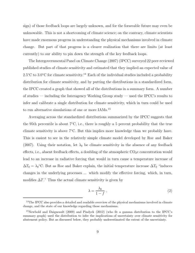
This is easiest to see in the relatively simple climate model developed by Roe and Baker
(2007). Using their notation, let λ0 be climate sensitivity in the absence of any feedback
effects, i.e., absent feedback effects, a doubling of the atmospheric CO2e concentration would
lead to an increase in radiative forcing that would in turn cause a temperature increase of
∆T0 = λ0◦C. But as Roe and Baker explain, the initial temperature increase ∆T0 “induces
changes in the underlying processes ... which modify the effective forcing, which, in turn,
modifies ∆T .” Thus the actual climate sensitivity is given by
λ =λ0
1 − f, (2)
14The IPCC also provides a detailed and readable overview of the physical mechanisms involved in climatechange, and the state of our knowledge regarding those mechanisms.
15Newbold and Daigneault (2009) and Pindyck (2012) (who fit a gamma distribution to the IPCC’ssummary graph) used the distribution to infer the implications of uncertainty over climate sensitivity forabatement policy. But as discussed below, they probably underestimated the extent of the uncertainty.
9

where f (0 ≤ f ≤ 1) is the total feedback factor (which in a more complete and complex
model would incorporate several feedback effects).
Unfortunately, we don’t know the value of f . Roe and Baker point out that if we knew
the mean and standard deviation of f , denoted by f and σf respectively, and if σf is small,
then the standard deviation of λ would be proportional to σf/(1 − f)2. Thus uncertainty
over λ is greatly magified by uncertainty over f , and becomes very large if f is close to 1.
Likewise, if the true value of f is close to 1, climate sensitivity would be huge.
As an illustrative exercise, Roe and Baker assume that f is normally distributed (with
mean f and standard deviation σf), and derive the resulting distribution for λ, climate sen-
sitivity. Given their choice of f and σf , the resulting median and 95th percentile are close to
the corresponding numbers that come from averaging across the standardized distributions
summarized by the IPCC.16 The Interagency Working Group calibrated the Roe-Baker dis-
tribution to fit the composite IPCC numbers more closely, and then applied that distribution
to each of the three IAMs as a way of analyzing the sensitivity of their SCC estimates to
uncertainty over climate sensitivity.
Given the limited available information, the Interagency Working Group did the best
it could. But it is likely that they — like others who have used IAMs to analyze climate
change policy — have understated our uncertainty over climate sensitivity. We don’t know
whether the feedback factor f is in fact normally distributed (nor do we know its mean and
standard deviation). Roe and Baker simply assumed a normal distribution. In fact, in an
accompanying article in the journal Science, Allen and Frame (2007) argued that climate
sensitivity is in the realm of the “unknowable.”
16The Roe-Baker distribution is given by:
g(λ; f , σf , θ) =1
σf
√2πz2
exp
[
−1
2
(
1 − f − 1/z
σf
)2]
,
where z = λ + θ. The parameter values are f = 0.797, σf = .0441, θ = 2.13. This distribution is fat-tailed,i.e., declines to zero more slowly than exponentially. Weitzman (2009) has shown that parameter uncertaintycan lead to a fat-tailed distribution for climate sensitivity, and that this implies a relatively high probabilityof a catastrophic outcome, which in turn suggests that the value of abatement is high. Pindyck (2011a)shows that a fat-tailed distribution by itself need not imply a high value of abatement.
10

3.2 The Damage Function
When assessing climate sensitivity, we at least have scientific results to rely on, and can
argue coherently about the probability distribution that is most consistent with those results.
When it comes to the damage function, however, we know almost nothing, so developers of
IAMs can do little more than make up functional forms and corresponding parameter values.
And that is pretty much what they have done.
Most IAMs (including the three that were used by the Interagency Working Group to
estimate the SCC) relate the temperature increase T to GDP through a “loss function”
L(T ), with L(0) = 1 and L′(T ) < 0. Thus GDP at time t is GDPt = L(Tt)GDP′
t, where
GDP′
t is what GDP would be if there were no warming. For example, the Nordhaus (2008)
DICE model uses the following inverse-quadratic loss function:
L = 1/[1 + π1T + π2(T )2] . (3)
Weitzman (2009) suggested the exponential-quadratic loss function:
L(T ) = exp[−β(T )2] , (4)
which allows for greater losses when T is large. But remember that neither of these loss
functions is based on any economic (or other) theory. Nor are the loss functions that appear
in other IAMs. They are just arbitrary functions, made up to describe how GDP goes down
when T goes up.
The loss functions in PAGE and FUND, the other two models used by the Interagency
Working Group, are more complex but equally arbitrary. In those models, losses are calcu-
lated for individual regions and (in the case of FUND) individual sectors, such as agriculture
and forestry. But there is no pretense that the equations are based on any theory. When
describing the sectoral impacts in FUND, Tol (2002b) introduces equations with the words
“The assumed model is:” (e.g., pages 137–139, emphasis mine), and at times acknowledges
(p. 142) that “The model used here is therefore ad hoc.”
The problem is not that IAM developers were negligent and ignored economic theory;
there is no economic theory that can tell us what L(T ) should look like. If anything, we
11

would expect T to affect the growth rate of GDP, and not the level. Why? First, some effects
of warming will be permanent; e.g., destruction of ecosystems and deaths from weather
extremes. A growth rate effect allows warming to have a permanent impact. Second, the
resources needed to counter the impact of warming will reduce those available for R&D and
capital investment, reducing growth.17 Third, there is some empirical support for a growth
rate effect. Using data on temperatures and precipitation over 50 years for a panel of 136
countries, Dell, Jones and Olken (2012) have shown that higher temperatures reduce GDP
growth rates but not levels. Likewise, using data for 147 countries during 1950 to 2007,
Bansal and Ochoa (2011, 2012) show that increases in temperature have a negative impact
on economic growth.18
Let’s put the issue of growth rate versus level aside and assume that the loss function of
eqn. (3) is a credible description of the economic impact of higher temperatures. Then the
question is how to determine the values of the parameters π1 and π2. Theory can’t help us,
nor is data available that could be used to estimate or even roughly calibrate the parameters.
As a result, the choice of values for these parameters is essentially guesswork. The usual
approach is to select values such that L(T ) for T in the range of 2◦C to 4◦C is consistent
with common wisdom regarding the damages that are likely to occur for small to moderate
increases in temperature. Most modelers choose parameters so that L(1) is close to 1 (i.e.,
no loss), L(2) is around .99 or .98, and L(3) or L(4) is around .98 to .96. Sometimes these
numbers are justified by referring to the IPCC or related summary studies. For example,
Nordhaus (2008) points out (page 51) that the 2007 IPCC report states that “global mean
losses could be 1–5% GDP for 4◦C of warming.” But where did the IPCC get those numbers?
17Adaptation to rising temperatures is equivalent to the cost of increasingly strict emission standards,which, as Stokey (1998) has shown with an endogenous growth model, reduces the rate of return on capitaland lowers the growth rate. To see this, suppose total capital K = Kp + Ka(T ), with K′
a(T ) > 0, whereKp is directly productive capital and Ka(T ) is capital needed for adaptation to the temperature increase T(e.g., stronger retaining walls and pumps to counter flooding, more air conditioning and insulation, etc.).If all capital depreciates at rate δK , Kp = K − Ka = I − δKK − K′
a(T )T , so the rate of growth of Kp isreduced. See Brock and Taylor (2010) and Fankhauser and Tol (2005) for related analyses.
18See Pindyck (2011b, 2012) for further discussion and an analysis of the policy implications of a growthrate versus level effect. Note that a climate-induced catastrophe, on the other hand, could reduce both thegrowth rate and level of GDP.
12
From its own survey of several IAMs. Yes, it’s a bit circular.
The bottom line here is that the damage functions used in most IAMs are completely
made up, with no theoretical or empirical foundation. That might not matter much if we are
looking at temperature increases of 2 or 3◦C, because there is a rough consensus (perhaps
completely wrong) that damages will be small at those levels of warming. The problem is
that these damage functions tell us nothing about what to expect if temperature increases
are larger, e.g., 5◦C or more.19 Putting T = 5 or T = 7 into eqn. (3) or (4) is a completely
meaningless exercise. And yet that is exactly what is being done when IAMs are used to
analyze climate policy.
I do not want to give the impression that economists know nothing about the impact
of climate change. On the contrary, considerable work has been done on specific aspects of
that impact, especially with respect to agriculture. One of the earliest studies of agricultural
impacts, including adaptation, is Mendelsohn, Nordhaus and Shaw (1994); more recent ones
include Deschenes and Greenstone (2007) and Schlenker and Roberts (2009). A recent study
that focuses on the impact of climate change on mortality, and our ability to adapt, is
Deschenes and Greenstone (2011). And recent studies that use or discuss the use of detailed
weather data include Dell, Jones and Olken (2012) and Auffhammer et al. (2013). These are
just a few examples; the literature is large and growing.
Statistical studies of this sort will surely improve our knowledge of how climate change
might affect the economy, or at least some sectors of the economy. But the data used in these
studies are limited to relatively short time periods and small fluctuations in temperature and
other weather variables — the data do not, for example, describe what has happened over
20 or 50 years following a 5◦C increase in mean temperature. Thus these studies cannot
enable us to specify and calibrate damage functions of the sort used in IAMs. In fact, those
damage functions have little or nothing to do with the detailed econometric studies related
19Some modelers are aware of this problem. Nordhaus (2008) states (p. 51): “The damage functionscontinue to be a major source of modeling uncertainty in the DICE model.” To get a sense of the wide rangeof damage numbers that come from different models, even for T = 2 or 3◦C, see Table 1 of Tol (2012). Stern(2013) argues that IAM damage functions ignore a variety of potential climate impacts, including possiblycatastrophic ones.
13

to agricultural and other specific impacts.
4 Catastrophic Outcomes
Another major problem with using IAMs to assess climate change policy is that the models
ignore the possibility of a catastrophic climate outcome. The kind of outcome I am referring
to is not simply a very large increase in temperature, but rather a very large economic effect,
in terms of a decline in human welfare, from whatever climate change occurs. That such
outcomes are ignored is not surprising; IAMs have nothing to tell us about them. As I
explained, IAM damage functions, which anyway are ad hoc, are calibrated to give small
damages for small temperature increases, and can say nothing meaningful about the kinds
of damages we should expect for temperature increases of 5◦C or more.
4.1 Analysis of Catastrophic Outcomes.
For climate scientists, a “catastrophe” usually takes the form of a high temperature outcome,
e.g., a 7◦C or 8◦C increase by 2100. Putting aside the difficulty of estimating the probability
of that outcome, what matters in the end is not the temperature increase itself, but rather
its impact. Would that impact be “catastrophic,” and might a smaller (and more likely)
temperature increase be sufficient to have a catastrophic impact?
Why do we need to worry about large temperature increases and their impact? Because
even if a large temperature outcome has low probability, if the economic impact of that
change is very large, it can push up the SCC considerably. As discussed in Pindyck (2013a),
the problem is that the possibility of a catastrophic outcome is an essential driver of the SCC.
Thus we are left in the dark; IAMs cannot tell us anything about catastrophic outcomes,
and thus cannot provide meaningful estimates of the SCC.
It is difficult to see how our knowledge of the economic impact of rising temperatures
is likely to improve in the coming years. More than temperature change itself, economic
impact may be in the realm of the “unknowable.” If so, it would make little sense to try to
use an IAM-based analysis to evaluate a stringent abatement policy. The case for stringent
14

abatement would have to be based on the (small) likelihood of a catastrophic outcome in
which climate change is sufficiently extreme to cause a very substantial drop in welfare.
4.2 What to Do?
So how can we bring economic analysis to bear on the policy implications of possible catas-
trophic outcomes? Given how little we know, a detailed and complex modeling exercise is
unlikely to be helpful. (Even if we believed the model accurately represented the relevant
physical and economic relationships, we would have to come to agreement on the discount
rate and other key parameters.) Probably something simpler is needed. Perhaps the best
we can do is come up with rough, subjective estimates of the probability of a climate change
sufficiently large to have a catastrophic impact, and then some distribution for the size of
that impact (in terms, say, of a reduction in GDP or the effective capital stock).
The problem is analogous to assessing the world’s greatest catastrophic risk during the
Cold War — the possibility of a U.S.-Soviet thermonuclear exchange. How likely was such
an event? There were no data or models that could yield reliable estimates, so analyses
had to be based on the plausible, i.e., on events that could reasonably be expected to play
out, even with low probability. Assessing the range of potential impacts of a thermonuclear
exchange had to be done in much the same way. Such analyses were useful because they
helped evaluate the potential benefits of arms control agreements.
The same approach might be used to assess climate change catastrophes. First, consider
a plausible range of catastrophic outcomes (under, for example, BAU), as measured by
percentage declines in the stock of productive capital (thereby reducing future GDP). Next,
what are plausible probabilities? Here, “plausible” would mean acceptable to a range of
economists and climate scientists. Given these plausible outcomes and probabilities, one can
calculate the present value of the benefits from averting those outcomes, or reducing the
probabilities of their occurrence. The benefits will depend on preference parameters, but
if they are sufficiently large and robust to reasonable ranges for those parameters, it would
support a stringent abatement policy. Of course this approach does not carry the perceived
precision that comes from an IAM-based analysis, but that perceived precision is illusory.
15

To the extent that we are dealing with unknowable quantities, it may be that the best we
can do is rely on the “plausible.”
5 Conclusions.
I have argued that IAMs are of little or no value for evaluating alternative climate change
policies and estimating the SCC. On the contrary, an IAM-based analysis suggests a level of
knowledge and precision that is nonexistent, and allows the modeler to obtain almost any
desired result because key inputs can be chosen arbitrarily.
As I have explained, the physical mechanisms that determine climate sensitivity involve
crucial feedback loops, and the parameter values that determine the strength of those feed-
back loops are largely unknown. When it comes to the impact of climate change, we know
even less. IAM damage functions are completely made up, with no theoretical or empiri-
cal foundation. They simply reflect common beliefs (which might be wrong) regarding the
impact of 2◦C or 3◦C of warming, and can tell us nothing about what might happen if the
temperature increases by 5◦C or more. And yet those damage functions are taken seriously
when IAMs are used to analyze climate policy. Finally, IAMs tell us nothing about the
likelihood and nature of catastrophic outcomes, but it is just such outcomes that matter
most for climate change policy. Probably the best we can do at this point is come up with
plausible estimates for probabilities and possible impacts of catastrophic outcomes. Doing
otherwise is to delude ourselves.
My criticism of IAMs should not be taken to imply that because we know so little,
nothing should be done about climate change right now, and instead we should wait until
we learn more. Quite the contrary. One can think of a GHG abatement policy as a form of
insurance: society would be paying for a guarantee that a low-probability catastrophe will
not occur (or is less likely). Some have argued that on precautionary grounds, there is a case
for taking the Interagency Working Group’s $21 (or updated $33) number as a rough and
politically acceptable starting point and imposing a carbon tax (or equivalent policy) of that
16

amount.20 This would help to establish that there is a social cost of carbon, and that social
cost must be internalized in the prices that consumers and firms pay. (Yes, most economists
already understand this, but politicians and the public are a different matter.) Later, as we
learn more about the true size of the SCC, the carbon tax could be increased or decreased
accordingly.
20See, for example, Pindyck (2013b) and Litterman (2013). National Research Council (2011) comes to asimilar conclusion.
17
References
Allen, Myles R., and David J. Frame. 2007. “Call Off the Quest.” Science, 318: 582–583.
Auffhammer, Maximilian, Solomon M. Hsiang, Wolfram Schlenker, and Adam
Sobel. 2013. “Using Weather Data and Climate Model Output in Economic Analysis of
Climate Change.” National Bureau of Economic Research Working Paper 19087.
Bansal, Ravi, and Marcelo Ochoa. 2011. “Welfare Costs of Long-Run Temperature
Shifts.” National Bureau of Economic Research Working Paper 17574.
Bansal, Ravi, and Marcelo Ochoa. 2012. “Temperature, Aggregate Risk, and Expected
Returns.” National Bureau of Economic Research Working Paper 17575.
Brock, William A., and M. Scott Taylor. 2010. “The Green Solow Model.” Journal of
Economic Growth.
Cai, Yongyang, Kenneth L. Judd, and Thomas S. Lontzek. 2013. “The Social Cost
of Stochastic and Irreversible Climate Change.” National Bureau of Economic Research
Working Paper 18704.
Dell, Melissa, Benjamin F. Jones, and Benjamin A. Olken. 2012. “Temperature
Shocks and Economic Growth: Evidence from the Last Half Century.” American Economic
Journal: Macroeconomics, 4: 66–95.
Deschenes, Olivier, and Michael Greenstone. 2007. “The Economic Impact of Cli-
mate Change: Evidence from Agricultural Output and Random Fluctuations in Weather.”
American Economic Review, 97(1): 354–385.
Deschenes, Olivier, and Michael Greenstone. 2011. “Climate Change, Mortality, and
Adaptation: Evidence from Annual Fluctuations in Weather in the US.” American Eco-
nomic Journal: Applied Economics, 3: 152–185.
Fankhauser, Samuel, and Richard S. J. Tol. 2005. “On Climate Change and Economic
Growth.” Resource and Energy Economics, 27: 1–17.
Gollier, Christian. 2013. Pricing the Planet’s Future. Princeton University Press.
Greenstone, Michael, Elizabeth Kopits, and Ann Wolverton. 2011. “Estimating the
Social Cost of Carbon for Use in U.S. Federal Rulemakings: A Summary and Interpreta-
tion.” National Bureau of Economic Research Working Paper 16913.
Heal, Geoffrey. 2009. “Climate Economics: A Meta-Review and Some Suggestions.” Re-
view of Environmental Economics and Policy, 3: 4–21.
18

Hope, C.W. 2006. “The Marginal Impact of CO2 from PAGE 2002: An Integrated As-
sessment Model Incorporating the IPCC’s Five Reasons for Concern.” The Integrated
Assessment Journal, 6: 19–56.
Interagency Working Group on Social Cost of Carbon. 2010. “Technical Support
Document: Social Cost of Carbon for Regulatory Impact Analysis.” U.S. Government.
Interagency Working Group on Social Cost of Carbon. 2013. “Technical Support
Document: Technical Update of the Social Cost of Carbon for Regulatory Impact Analy-
sis.” U.S. Government.
Intergovernmental Panel on Climate Change. 2007. Climate Change 2007. Cambridge
University Press.
Kelly, David L., and Charles D. Kolstad. 1999. “Bayesian Learning, Growth, and
Pollution.” Journal of Economic Dynamics and Control, 23: 491–518.
Litterman, Bob. 2013. “What Is the Right Price for Carbon Emissions?” Regulation,
36(2): 38–43.
Mendelsohn, Robert. 2008. “Is the Stern Review an Economic Analysis?” Review of
Environmental Economics and Policy, 2: 45–60.
Mendelsohn, Robert, William D. Nordhaus, and Daigee Shaw. 1994. “The Impact
of Global Warming on Agriculture: A Ricardian Analysis.” American Economic Review,
84(4): 753–771.
National Research Council. 2011. America’s Climate Choices. Washington,
D.C.:National Academies Press.
Newbold, Stephen C., and Adam Daigneault. 2009. “Climate Response Uncertainty
and the Expected Benefits of Greenhouse Gas Emissions Reductions.” Environmental and
Resource Economics, 44: 351–377.
Nordhaus, William D. 1991. “To Slow or Not to Slow: The Economics of the Greenhouse
Effect.” Economic Journal, 101: 920–937.
Nordhaus, William D. 1993a. “Optimal Greenhouse Gas Reductions and Tax Policy in
the ’DICE’ Model.” American Economic Review, 83: 313–317.
Nordhaus, William D. 1993b. “Rolling the ’DICE’: An Optimal Transition Path for Con-
trolling Greenhouse Gases.” Resource and Energy Economics, 15: 27–50.
Nordhaus, William D. 2007. “A Review of the Stern Review on the Economics of Climate
Change.” Journal of Economic Literature, 686–702.
19
Nordhaus, William D. 2008. A Question of Balance: Weighing the Options on Global
Warming Policies. Yale University Press.
Nordhaus, William D. 2011. “Estimates of the Social Cost of Carbon: Background and
Results from the RICE-2011 Model.” National Bureau of Economic Research Working
Paper 17540.
Pindyck, Robert S. 2011a. “Fat Tails, Thin Tails, and Climate Change Policy.” Review
of Environmental Economics and Policy, 5(2): 258–274.
Pindyck, Robert S. 2011b. “Modeling the Impact of Warming in Climate Change Eco-
nomics.” In The Economics of Climate Change: Adaptations Past and Present. , ed. G.
Libecap and R. Steckel. University of Chicago Press.
Pindyck, Robert S. 2012. “Uncertain Outcomes and Climate Change Policy.” Journal of
Environmental Economics and Management, 63: 289–303.
Pindyck, Robert S. 2013a. “The Climate Policy Dilemma.” Review of Environmental
Economics and Policy, 7.
Pindyck, Robert S. 2013b. “Pricing Carbon When We Don’t Know the Right Price.”
Regulation, 36(2): 43–46.
Roe, Gerard H., and Marcia B. Baker. 2007. “Why is Climate Sensitivity So Unpre-
dictable?” Science, 318: 629–632.
Schlenker, Wolfram, and Michael J. Roberts. 2009. “Nonlinear Temperature Effects
Indicate Severe Damages to U.S. Crop Yields under Climate Change.” Proceedings of the
National Academy of Sciences, 106(37): 15594–15598.
Stern, Nicholas. 2007. The Economics of Climate Change: The Stern Review. Cambridge
University Press.
Stern, Nicholas. 2008. “The Economics of Climate Change.” American Economic Review,
98: 1–37.
Stern, Nicholas. 2013. “The Structure of Economic Modeling of the Potential Impacts
of Climate Change Has Grafted Gross Underestimation onto Already Narrow Science
Models.” Journal of Economic Literature, 51: ??–??
Stokey, Nancy. 1998. “Are There Limits to Growth?” International Economic Review,
39: 1–31.
Tol, Richard S. J. 2002a. “Estimates of the Damage Costs of Climate Change, Part I:
Benchmark Estimates.” Environmental and Resource Economics, 21: 47–73.
20

Tol, Richard S. J. 2002b. “Estimates of the Damage Costs of Climate Change, Part II:
Dynamic Estimates.” Environmental and Resource Economics, 21: 135–160.
Tol, Richard S.J. 2012. “Targets for Global Climate Policy: An Overview.” Draft working
paper.
Weitzman, Martin L. 2007. “A Review of the Stern Review on the Economics of Climate
Change.” Journal of Economic Literature, 703–724.
Weitzman, Martin L. 2009. “On Modeling and Interpreting the Economics of Catastrophic
Climate Change.” Review of Economics and Statistics, 91: 1–19.
Weitzman, Martin L. 2013. “Tail-Hedge Discounting and the Social Cost of Carbon.”
Journal of Economic Literature, 51: ??–??
21


