Download - CMMI High Maturity Hand Book


CMMI High Maturity Handbook
VishnuVarthanan Moorthy
Copyright 2015 VishnuVarthanan Moorthy

Contents
High Maturity an Introduction
Prerequisites for High Maturity
Planning High Maturity Implementation
SMART Business Objectives and Aligned Processes
Measurement System and Process Performance Models
Process Performance Baselines
Define and Achieve Project Objectives and QPPOs
Causal Analysis in Projects to Achieve Results
Driving Innovation/Improvements to Achieve Results
Succeeding in High Maturity Appraisals
Reference Books, Links and Contributors

High Maturity an Introduction
CMMI High Maturity Level is one of the Prestigious Rating any IT/ITES Companies would be interested
in getting. The Maturity Level 4 and 5 achievement is considered as High Maturity as the Organizations
understand their own performance and Process performance. In addition they bring world class practices
to improve the Process Performance to meet their Business Needs. CMMI Institute has kept very high
standards in appraisals to ensure that stringent evaluations are done before announcing the rating.
Similarly the practices given at Level 4 and Level 5 are having high integrity and complete alignment
with each other to stimulate Business Performance. Hence it’s become every Organizations interest to
achieve High Maturity Levels and also when they see the competitor is already been appraised at that
level, it becomes vital from marketing point of view to prove their own process Maturity. The ratings are
given for the processes and not for product or services. Hence a High Maturity Organization means, that
they are having better equipped processes to deliver results.
Why not every Organization go for Maturity Level 5 is a question which is there in our mind for quite
some time. It becomes difficult because the understanding on High Maturity expectations are less in many
organizations, advanced quality concepts, statistical usage expectations, longer cycles to see results, etc
are some of the reasons which prevents organizations. In 2006 when I was an Appraisal Team Member
looking at evidences for Maturity Level 5, myself and the Lead Appraiser has mapped the Scatter plot of
Effort Variance vs Size for Process Performance Model. After 9 years when we look back, the Industry
has moved on and does the CMMI Model V1.3. There is much better clarity on what do we expected to
do CMMI High Maturity. Similarly in 2007 there was a huge demand for Statistics Professors in
Organizations which goes for CMMI High Maturity and some organizations have recruited Six sigma
Black belts to do CMMI High Maturity Implementation. There was huge stress on applying statistics in
its best of form in organizations than the business results achievement. However with CMMI V.3 model
release CMMI Institute (then “SEI”) has ensured that it provides many clarifications materials, it grades
the Lead Appraisers as High Maturity Lead Appraiser, conducts regular workshops by which many
people in Industry has Benefitted with adequate details on what is expected as CMMI High Maturity
Organization. However still there is concern that this knowledge has not reached many upcoming. Small
and medium sector companies as intended. Also in bigger organizations when they achieve ML4 or ML5
only a limited set of people work on this and/or in a particular function of the implementation they work.
These factors reduces the number of people who can actually interpret ML5 without any assistance. This
also means very few organizations are within comfort zones of High Maturity.
The Purpose of this book is to give insight about High Maturity Implementation and how to interpret the
practices in real life conditions of an organization. The Book is written from Implementation point of
view and not from technical expectations point of view. The usage of CMMI word is trademark of CMMI
Institute, similarly the contents of the CMMI model wherever we refer in this book is for Reference
purpose only and its copyright material of CMMI. I would recommend you to refer “CMMI
Implementation Guide” book along with this book for understanding up to CMMI ML3 practices and its
implementation. This book deals only with CMMI Maturity Level 4 and 5 practices. I have tried covering
CMMI Development model and Services model implementation in this book.

High Maturity Organizations has always been identified with their ability to understand the past
quantitatively, manage the current performance quantitatively and predict the future quantitatively. High
Maturity Organizations always maintains traceability with their business objectives with Process
Objectives and manage the process. In addition they measure Business results and compare with their
objectives and perform suitable improvements. However even a Maturity Level 3 organization can also
maintain such traceability and measure their business results, which is the need of the hour in Industry. I
am sure CMMI Institute will consider this need.
In addition there is a growing need of engagement level benchmarking which clients are interested. The
client wants to know whether their projects have been handled with best of the process and what is the
grading/rating can be given. The current Model of CMMI is more suitable for Organizational
unit/Enterprise wide appraisals, however engagement level rating needs better design or new
recommendation on how do the process areas are selected and used. In high maturity Organizations we
can see the use of prediction model and few specific Process areas being used by many organization to
demonstrate engagement level maturity. Many a times they miss out the Business objectives and client
objectives traceability to Engagement Objectives and from there how they are achieved. There is a
growing need for Engagement level Maturity assessment from users.
In High Maturity Organizations we typically see a number of Process Performance Baselines, Process
Performance Models, Causal analysis Reports, Innovation Boards and capable Process to deliver Results.
In this book we will see about all these components and how they are created. The flow the book is
designed in that way, where we go by the natural implementation steps ( in a way you can make your
implementation schedule accordingly) and then end of the relevant chapters, we will indicate which
process area and what are the specific practices are covered in it. However you may remember the goals
have to be achieved and practices are expected components only. Similarly we will not be explaining the
Generic Practices, as you may read the same in “CMMI Implementation Guide” book. Also there is a
detailed book only on “Process performance Models - Statistical, Probabilistic and simulation” which
details on various methods by which process performance models can be developed with detailed step. I
would recommend to refer this book, if you want to do something more than regression based model
given in this book. Also for the beginners and practitioners in quality, to refresh and learn different
techniques in quality assurance field, you can choose to refer “Jumpstart to Software Quality Assurance”
book.
Let’s start our High Maturity Journey Now!

Prerequisites for CMMI High Maturity
CMMI High Maturity in an organization is not an automatic progress which they can attain by doing
more or increasing coverage of processes; it’s a paradigm shift in the way the organization works and
project management practices. CMMI High maturity is an enabler and a sophisticated tool in your hand to
predict your performance and improve your certainty. It’s like using a GPS or Navigational system while
driving, isn’t great! Yes, however the GPS and Navigational system for you will not be procured, instead
you need to develop. Once you develop and maintain it, it’s sure that you will reach your target in
predictable manner.
In order to implement CMMI High Maturity in any Organization, the Organizations should meet certain
prerequisites, which can make their journey easier,
*Strong Measurement Culture and reporting System
*Detailed Work Break Down Structures and/or detailed tracking tool of services
*Good Project management tool
*Strong Project management Knowledge
*Regular Reviews by Senior management
*Good understanding on tailoring and usage
*Established Repositories for integrated project management tool
*Strong SEPG team with good analytical Skills
*Statistical and Quantitative understanding with project managers and SQA’s (if needed, can be trained)
*Budget for Investing on Statistical and management tools and their deployment
*Good Auditing System and escalation resolution
What it’s not:
*Not a diamond ornament to flash
*Not a competitors demand or client demand
*Not one of colorful certification in reception area
*Not an Hifi language to use
*Not a prestigious medal to wear
*Not a statistical belt to be proud
What it is:
*A performance enhancing tool for your organization to achieve results
*Makes you align your business Objectives with project objectives
*Statistical concepts add to certainty and better control and removes false interpretations
*It makes you competitive against your competitors
*A Maturity Level in which you maintain the maturity towards reacting to changes
If you believe that by spending twice or thrice the money of your CMMI ML3 implementation you can
achieve High Maturity, then you may be making a big mistake! Not because it may never be possible, but
you just lost the intent. Unfortunately today not many realize it, but they want to show their arm strength
to the world by have CMMI Ml5. However it’s a real good model at L3 itself, which can do wonders for
you. Why to fit a car which travel in countryside with autopilot equipment, do you need it, please choose.

High Maturity practices are the near classic improvements made in software process industry in a decade
or so. At this moment this is the best you can get , if applied well! Not many models and standards have
well thought about maturity and application of best practices, as given in CMMI ML5 Model. So if you
really want to improve and be a world class organization by true sense, just close your eyes and travel this
path, as its extremely pleasant in its own way!

Planning High Maturity Implementation
Scoping Implementation:
Do we need CMMI in every hook and corner of your Organization or the places where you feel you get
better Return of Investment is possible, is your first Decision. As an user your organization can decide to
implement CMMI practices on enterprise wide and may do appraisal within a particular scope
(Organizational unit scope). At this moment Tata Consultancy Services has done enterprise wide
appraisal, which is one of the largest Organizational unit with maximum number of people across
multiple countries. But not every Organization need to follow that path and its free for the user
organization to decide which parts of your enterprise may need CMMI with particular Maturity level.
Within an Organization there can be two different Maturity Level the organization may want to achieve
for certain reasons, are also possible. In such case the factors like Criticality of Business, Stability in
Performance, Unit Size (smaller or Larger), Dependencies with Internal/external sources, Type of
Business (Staffing/Owning service or Development), Cycle of delivery (Shorter/longer,etc), people
Competency, Existing Lifecycles and Lenient Methods usage, Technology used etc can determine do you
really need CMMI High Maturity Level 5. Sometimes it could be only the expectation of your client to
show your process maturity, however you may confident that you are already performing at a maturity
level 5 or in optimizing mode. So you may choose to implement/validate the CMMI practices for a
particular scope using CMMI Material and CMMI Appraisal (SCAMPI A). What happens if you are a
25000 member organization, which decides to implement CMMI HM for a division which has only 1500
members is that fine? Can you perform an appraisal and say you are at ML 5? Yes, it is. CMMI Model is
not developed for marketing purpose or for an enterprise wide appraisal purpose. It’s developed to
improve your delivery through Process improvements, hence if you decide to use it in a small part of
organization, its up to you. The scope in which CMMI is Implemented is “Organizational Unit”, which
has its own definition of Type of work, Locations covered, people and functions involved, type of clients
serviced, etc. This boundary definition is a must when it comes to appraisal scope, however the same
definition when you use in implementation time will give greater focus to the Organization. The
Organizational Unit can be of equivalent description of the Organization, if you choose the entire business
units and functions within your Organization. However there are instances where the Organization claims
its overall ML5 with smaller Organizational Unit (Less than Organization), which is not acceptable. The
CMMI Institute has published appraisal results site, where the clients can see the Organizations’ real
scope of Appraisal (implementation scope could be larger than this) and verify whether the business
centre and practices of supplier are part of this scope.
From an Organization which implements CMMI High Maturity Practices, we may need to consider the
business objectives and its criticality, where systematic changes are possible and measurable, where
clients wants us to consider improvements, which are the activities we can control and where we can
influence, where we feel improvements are possible and currently we observe failures and/or wastages.
Selection of HMLA and Consultants:
This is activity plays an important role in your CMMI ML5 Journey, after all there are many places in
CMMI its subject to the interpretation of your HMLA and consultant. High Maturity Lead Appraiser
(HMLA) are certified by CMMI Institute and only they can do an Appraisal and announce result of an
Organization as Maturity Level 4 or 5. When you start your long journey which varies from 1.5 years to 3

years typically, your effort is going to be shaped most often by your HMLA and Consultant. Their
presence with you should be beneficial in terms of improving your process there by achieving business
results.
Hence when selecting your HMLA and Consultant, its important to check, how many organizations they
have supported to successfully to achieve CMMI High Maturity in the last 2 years. Do they have
experience in your type of business or they have earlier assisted/performed CMMI activities to a similar
organization like yours. This will help you to get an idea on what you will be getting from them as
guidance in future. Less experience is always a risk, as your team also might be needing some good
guidance and review points to look. Check the geographic locations served by them and communication
abilities in your native language also an important aspect, when your organizational presence is limited to
a particular region and your people are not comfortable with foreign language. Also this will help in quick
settling of consultant and HMLA to your culture.
There are HMLA’s who has never done any High Maturity Appraisals in the past, but have cleared the
eligibility criteria of CMMI Institute and been certified many years ago. They have also been able to
renew their certificates based on their work on research, active participation on formal forums/seminars of
CMMI Institute and been able to collect their renewal points. However their experience and comfort to
perform a SCAMPI A appraisal for you can’t be judged easily. This is a critical fact an organization has
to consider. The same for a consultant who has worked in the past for many CMMI ML2 and ML3
consulting, but not in High Maturity Level (ML4 and ML5), its difficult to deliver many a times. Hence a
special care to be given by your Organization in selecting your HMLA.
Similarly the working style of HMLAs differ and that has to be checked specific to your organizations.
Some of them looks at overall intention of the Goals and guide your team in interpreting it in a better way
and then pushes your team to achieve the target. However some of them looks at practice level aspects in
details and always questions your ability to interpret and implement the practice. Such style of working
may not really motivate your Organization and your team. Considering this a long journey with your
HMLA and Consultant, its important to understand their working style quickly and decide. Some
Organizations pay for Spot Checks/Reviews and then see their way of working before entering into final
agreement.
Similarly it’s important to see how well your consultant (if you have one) and your HMLAs getting
aligned. If they both work completely in isolation, that means there is more risk of final moment changes
coming from HMLA. Its always recommended to have frequent checks by HMLA to get confirmation on
the Process improvement path you have taken and its design. In the past we have seen Organizations do
lot of rework simply because they failed to involve HMLA’s in the intermediate checks and left only to
consultants. Also check if your Consultants at least have CMMI Associate Certification. In future there is
a possibility that CMMI Institute might announce certification as CMMI Professional or Specific to
consultants.
Scheduling CMMI HM Implementation:
Many organizations wants to achieve CMMI ML5 in 1.5 of years and there are few who understands the
natural cycle of it and ready for 2 to 3 years implementation. We shall remember the Maturity is a state
where we have industrialized practices and able to demonstrate capabilities, hence you need time to see

whether your organization performs in this state for some time. In addition, most of the practices have
interdependency with sequencing and not parallel activities. Above all, to achieve your Business Vision
and Targets with Process Maturity needs time to understand and improve processes. Hence anyone
implementing CMMI L4 and L5 in a period less than 1.5 year shall be studied for the best and worst.
The decision of timeline depends on factors like basic measurement structure, Process Culture, readiness
for improvements/resistance for improvements, People and technical capabilities and frequency of visible
outcomes and finally the time required to achieve Business Objectives (though it’s not mandatory to
demonstrate complete achievement). We would typically need a time period of 2 years to achieve the
High Maturity.
The Key Factors to be considered in making a Schedule for CMMI HM are,
*Number of Business Units/Delivery Teams are Involved
*Number of functions involved and Interdependencies ( Metrics, SEPG, SQA, IT Support, Logistics,
Training, Sr Management Teams, etc)
*Number of Business Objectives, QPPOs and Process Performance Models Required
*Possible Frequency of Process Performance Baselines(PPB) and Number of PPBs
*Current Level of Competency with Project Team, Quality Assurance and other vital teams and training
Requirements
*Level of Resistance to change and time required for change Management
*Intermediate Reviews by High Maturity Lead Appraiser
*Process Up gradation Time to meet HM Requirements
*Time between SCAMPI B/ Pre Appraisal to SCAMPI A
*Internal Appraisals by Organization
*Organizational Initiatives Cycle
*Client and supplier Dependencies, if any
*Time Needed for a core Team who possess the understanding of Business with CMMI and Statistical
Knowledge

CMMI Implementation structure:
Every Organization has an existing structure to delivery products or services, so why do we need to
discuss on this point, they just have to implement High Maturity Practices isn’t it? Its not that easy,
because learning of the model, interpretation to the job we do and application new techniques (statistics &
structured analysis) has to be demonstrated by these teams. Hence unless we have dedicated groups it
would be difficult to bring knowledge and interpretations to real life conditions. Moreover, the client or
neither we will be interested in making the Project managers and team to spend time and effort in the area
where they are not really that strong. By setting up CMMI core team we can concentrate our efforts and
bring the best and pass it to the Organization. The underlying needs in setting up CMMI Specific teams
are a) Scheduling and monitoring of the CMMI High Maturity Program b) BO, QPPO finalization with
Regular Monitoring of achievement and PCB preparation c) Process Performance Model development,
usage in projects, Sub process monitoring checks in projects d) Causal analysis application guidance to
projects e) Organizational Innovation/Improvement Initiatives running. These activities can be done by i)
one central core group formed in the organization or existing QA organization can take care of it or ii)
activities a, b, c is taken care by core group/QA group and d and e by a new group or there can be N
number of combination like these can be formed in teams based on your organizations existing structure.

However typically you need people with good quantitative and statistical understanding to drive the
activities relevant to Objectives fixing, PPM and PCB preparation, etc. Also people with good
understanding in engineering and Project management can be involved in causal analysis and in
Organizational Innovation activities to support the Performance of Organization to achieve Business
Objectives.
It’s important to ensure that there is clarity with every team in terms of Roles and Responsibilities and
their Interaction points. Also its important to ensure the project team has learnt High Maturity Practices
and they are able to use it effectively without much handholding from Quality Assurance or any other
teams.
Steering Committee
The High Maturity Program needs a big change in legacy and culture many a times. To achieve this a
committee with clear driving abilities and authority should be available in the Organization. Steering
Committee drives the program of High Maturity achievement by removing impediments and providing
necessary support. Typically Delivery Heads of Business Units, functions and Operations would be part
of it along with the CMMI Program Team. The Identified CMMI Program Manager can provide
information on various activities their status. The SEPG and Other Important functions will be
represented to make action plan to progress further. The Sponsor of the Program will be the chairperson
for the meetings. These meetings can happen on monthly/bimonthly basis.

Typically the following aspects at High Maturity can be discussed,
*Planned Milestone dates and current achievement details
*Involvement Need of stakeholders
*Competency Needs of Project teams and functions
*Selection of High Maturity Lead Appraiser and Managing Activities
*Resource Needs to Drive the Program
*Technology and Lifecycle updates Required in context
*QMS Update and Purpose
*Approval for Improvements/Innovations to pilot and to deploy
*Scoping Implementation
*Interaction points with Other Units/Functions and Support Needed
*Challenges and Issues in Implementation
*Appraisal Planning
*Support Needed Area in Implementing CMMI High Maturity

SMART Business Objectives and Aligned Processes
The Ultimate aim of any Business Organization is to earn profit and achieve its business results and
CMMI model is aligned to help you achieve the Business results. It provides you the strategic practices
which helps you to plan, monitor and manage your business results achievement using Process
Improvements. Process here refers to inclusion of people and technology, which means any initiative
running to improve people competency or Technological advancement is also considered part of Process
Improvement Journey. CMMI sets the expectation clear by asking for measurable business objectives,
which includes variation and targeted time. This is achieved by having SMART Business objectives.
SMART refers to Specific, Measurable, Attainable, Relevant and Time bound. Which means the
objectives to have specific definition, to have clear measure, possible to achieve target, relevant to your
business context and it has definite time period.
Before we move into explaining it with samples, how do these business objective originate is basically
from your vision. Every Business Organization has its vision to achieve and its typically in a few years’
time period. The Vision can only be achieved if your immediate business targets are aligned to it and you
keep progress towards them year on year. Hence typically the Business objectives have clear traceability
with Vision and it’s of a year or two time period. Vision can get changed when there is a major change in
business and market conditions, etc. in such scenario the Business Objectives have to be aligned with it.
However it may be uncommon.
Sample SMART Business Objectives:
*Customer Satisfaction Rating to be improve from current performance of mean 3.5 to new
performance mean 4.0 by maintaining Standard Deviation at 0.25 by End of 2016
*Operations Effectiveness Ratio to improve from Current performance of mean 70% to new
performance mean 80% by maintaining Standard Deviation 6 by End of 2016
Quality and Process Performance Objectives known as QPPO in CMMI High Maturity is the connecting
factor between Processes and Business Objectives of the Organization. They are the objectives which are
quality and process targets which are measurable in the lifecycle of Operations/project, which when
achieved will lead to business objective achievement. Typically the Business objectives may not be
directly measurable from projects or measurable at intermediate stages, which leads to difficulty in
controlling them. However QPPOs are intermediate or one of the few important component which
influences the final achievement of Business objectives. For example, Customer satisfaction results may
be collected in periodic intervals and at the end of project, however what may influence the customer
satisfaction is Defect rate in product/service, SLA met, etc. If we keep these quality and process targets in
a limit, you may most probably get better customer satisfaction. This is how QPPO works to achieve
Business Objectives. The word Quality is stressed to think in terms of Quality Targets in your projects
and not only process and cost related targets.
Sample Vision-Business Objectives and QPPOs,

In this Book, We are going to use two sample cases of Business Objectives and QPPO’s throughout, as
applicable. One Business Objective from Application Development and another from Application
maintenance Scenario. So for the Business Objective sample which we saw in last section, the following
could be the QPPOs,

BO-QPPO Relationship
The relationship has to be logically identified with group of relevant people. Then they can be weighted
across multiple QPPOs. The QPPO which is possible to collect and contribute to one or more Business
Objective and critical in nature is prioritized and selected. There can be many possible QPPO’s
contributing to given Business objectives, however the Organization has to do trade off to find the best
possible ones , so that cost of measuring and Predicting these QPPOs has good Return on
Investments(ROI).
Though we may start with simple logical relationship, we need to establish a quantitative/statistical
relationship of QPPO with BO to find it an effective tool to achieve the Business Objective. So if the data
available already then these relationships to be established early.
In the above sample given here, if we collected the data from various projects and the metrics are
available with us, we may plot them to understand the relationship to substantiate their logical
relationship.

When it’s not possible to get this level of detail at the beginning of your journey for all Business
objectives and QPPOs, you are expected to collect data and to build it. The relationship need not be
always linear in nature and also it can be mathematical relationship in some cases.
Once we understand the possible QPPO’s we need to evaluate them on selecting for future usage. Though
some of them could good measures for BO, they may not be easy and periodical to capture and analyse.
Some of them has influence of similar other QPPO’s and so on. Hence it’s expected to evaluate the
Business Benefit in selecting the QPPO along with their relationship with BOs.
A sample QPPO table is given below,

Business Priority
1 -High, 3-Medium, 5-Low
QPPO Correlation with B.O
1-High, 3 - Medium, 5- Low
QPPO Contribution field is ranked based on their contribution, and lower the value then more chance of
getting selected. However you may reject few QPPOs based on business and practical reasons, however it
should be a well thought out decision. Also the ranking of QPPO helps in sub optimization and which one
to give high importance.
Process Flow and Process/Sub Process Selection:
Once the QPPO’s are selected the next important step is to understand how the process system helps us to
achieve these QPPO’s and which Process and Sub Processes are critical and what factors to consider and
what measures to consider. Hence its important for us to have Process System Map with us, before getting
in to this step.

In our sample case, we are considering we have QPPO’s on Software Application Development and
Software Application Management/maintenance Lifecycles. Hence its important for us to Identify the
Processes and its Sub Process ( it could be a logical group of set of activities already defined in process)
and their configuration as part of Delivery. So it would be easier for us to understand how the
Process/Sub Process contributes to Business.
Here we can see the Release Process is not broken in to Sub Process but all other Processes are now
identified in terms of their Sub Process. Hence further analysis and attribute identification, etc will be
handled using these set of Process/Sub Process for the QPPO and Application Development Area.

Here Help Desk as a function performs certain action in assigning tickets to the Project team. However
the Incident Management Process is broken in to Sub Process and User Support Process also divided in to
Sub Process. It’s not necessary that every Process has to be split in to Sub Process. The Selection of Sub
Process is based on criticality, measurability, and logical relationship, interaction points with other
Process and Roles and Tools involved. Based on this we may choose to form sub processes in a given
process, as it’s not always denoted in the past in a new High Maturity Seeking Organizations.
Once the Sub Process is identified, it’s important to see what attributes of the Sub Process will be useful
in prediction and Controlling the final Results (QPPO). Also which attributes are controllable or possible
to monitor with thresholds. Based on existing process architecture and Logical Discussions the Process
and their contribution to QPPO with Measurable Attributes can be identified. Logically we may first want
to know the Quality, Cost, and Time Parameters of Sub Process and then find measures which will be
able to communicate the performance of them. For example in our case we have taken Defect Density as
QPPO, which means the Process/Sub Process which contributes to Defect Injection and Defect Detection
has to be selected for measuring and measures of Defect (direct measure) achieved through the process
and measures which rule the efficiency of those process (time spent, effort spent- Indirect measure) will
be our interest. Hence these has to be identified as Process Attributes to measure.

Values:
Yes with Logical & Statistical Relationship 1, Yes with Only Logical Relationship 0.5, No/NA 0
Selection Criteria:
At least 1 goal the Sub process should contribute and its overall value to be 1 or greater than that.
These are the Process and Sub Process Measures which will be helping us to understand and monitor the
QPPOs and by controlling these measures it would be possible to manage the results of identified QPPOs.
Having said that there could be many influencing factors a Process or process system have, which can
impact achievement of these sub process measures and QPPOs. Identification of these measures are
always tricky as it could be any factors pertaining to the lifecycle. Good brainstorming, root cause
analysis or why-Why techniques may reveal what are the underlying causes which influence the results.
These are probably the influencing factors which we may want to control to achieve results at process
level or even at QPPO Level.
In order to help us understand that, these factors are coming from multiple areas, the following X factor
selection matrix can help.

Identifying the X factor which influences Y Factor (QPPO’s) is performed logically first and then data
collected about these measures. The relationship is established between the X factors and Y factors. These
relationship can also be used as Process Performance Model, when it meets the expectation of PPM.
Which means not all statistical or probabilistic relationship will be used as PPM, however its necessary to
qualify a factor as X factor. We will see further details about PPM in the upcoming chapters.
What We Covered:
Organizational Process Performance:
SP 1.1 Establish Quality and Process Performance Objectives
SP 1.2 Select Processes
SP 1.3 Establish Process Performance Measures

Measurement System and Process Performance Models
Measurement System Importance
To build strong High Maturity Practices at a quick time, the existing measurement system plays a vital
role. They helps us to collect and use the relevant data with accuracy and precision. The following aspects
in a measurement system are the key,
*Operational Definition for Measures/Metrics
*Type of Data and Unit of Measurement Details
*Linkage with B.O or QPPO or Process/Sub Process
*Source of Data
*Collection of Data
*Review/Validation of Data
*Frequency of collection and Submission
*Representation of Data – Charts, Plot, Table, etc
*Analysis Procedure
*Communication of Results to Stakeholders
*Measurement Data Storage and Retrieval
*Group Responsible & Stakeholder Matrix
*Trained Professionals to manage Measurement System
For every Measure the Purpose of collection and its intended usage to made clear, so that adequate
support we can get from delivery teams and functions.
When the BO, QPPO and X factors are identified logically, sometimes the measurement data is available
with you, sometimes not. When the data is available its important to check the existing data is collected in
the expected manner and it has the unit which we want to have and no or less processing is required. If
not, we may have to design the measurements quickly and start collecting it from the Projects and
functions. Which means you may need to wait sometimes a month or two to collect the first level
measures and build relationships.
The purpose at ML5 shifts from controlling by milestones to in process/phase controls, which means from
lagging indicators to leading indicators. So we control the X factors and there by using their relationship
with Y (Process, QPPOs) we understand the certainty/level of Meeting Y. So we build relationship
models using the X factors and Y of past and/or current instance, which helps us to predict the Y.

Hence its important to have these X factor measures collected early in CMMI Ml5 implementation, that
sets up the basis for Process performance model building and thereafter usage by Projects. Its also
important to ensure there is Gauge R&R is done to ensure Repeatability and Reproducibility in
measurement system, so that false alarms can be avoided and concentrate effort usefully.
A clear ML2 Measurement System is the need for strong ML4 and ML4 Maturity and institutionalization
of ML5 Practices.
Modelling in CMMI
Process Performance Models in Information Technology Industry is pretty young concept even after
many models and standards described its need from prediction and control point of view. Especially
Capability Maturity Model Integrated call for it to assess an organization as Highly Matured
Organization.
In CMMI Model, the Process Area ‘Organization Process Performance’ calls for useful Process
Performance Model (PPM)s establishment (& calibration) and Quantitative Project Management and
Organizational Performance Management process areas gets more benefit by using these models to
predict or to understand the uncertainties , thereby helping in reducing risk by controlling relevant
process/sub processes.
The PPM’s are built to predict the Quality and Process Performance Objectives and sometimes to
Business Objectives (using integrated PPMs)
Modelling plays a vital role in CMMI in the name of Process Performance Models. In fact we have seen
Organizations decide on the goals and immediately starts looking at what are their Process Performance
Model. It’s also because of lack of options and clarity, considering in software the data points derived are
smaller in nature and also because of process variation.
Considering it’s a growing filed and many wants to learn the techniques which can be applied in IT
Industry, we have added the content in this chapter. At the end of the chapter you will be able to
appreciate your learning on new Process Performance Models in IT Industry and work on few samples.
Don’t forget to claim your free data set from us to try these models.
What are the Characteristics of a Good PPM?
One or more of the measureable attributes represent controllable inputs tied to a sub process to enable
performance of ―what-if analyses for planning, dynamic re-planning, and problem resolution.
Process performance models include statistical, probabilistic and simulation based models that predict
interim or final results by connecting past performance with future outcomes.
They model the variation of the factors, and provide insight into the expected range and variation of
Predicted results.

A process performance model can be a collection of models that (when combined) meet the criteria of a
process performance model.
The role of Simulation & Optimization
Simulation:
It’s an activity of studying the virtual behaviour of a system using the representative model / miniature by
introducing expected variations in the model factors / attributes.
Simulation helps us to achieve confidence on the results or to understand the uncertainty levels
Optimization:
In the context of Modelling, Optimization is a technique in which the model outcome can be
maximized/minimized or targeted by introducing variations in the factors (with/without constraints) and
using relevant Decision rules. The Values of factors for which the outcome meets the possible expected
values are used as target for planning/composing process/sub process. This helps us to plan for success.
Types of Models - Definitions
Physical Modelling:
The Physical state of a system is represented using the scaled dimensions with/without similar
components. As part of Applied Physics we could see such models coming up often. Example: Prototype
of a bridge, a Satellite map, etc
Mathematical Modelling:
With the help of data the attributes of interest are used to form the representation of a system. Often these
models are used when people involved largely in making the outcome or the outcome is not possible to be
replicated in laboratory. Example: Productivity model, Storm Prediction, Stock market prediction, etc
Process Modelling:
The Entire flow of Process with factors and conditions are modelled. Often these models are useful in
understanding the bottlenecks in the process / system and to correct. Ex: Airport queue prediction, Supply
chain prediction, etc
Tree of Models

Process of Modelling

Modelling under our purview
We will see the following models in this chapter
Regression Based Models
Bayesian Belief Networks
Neural Networks
Fuzzy Logic
Reliability Modelling
Process Modelling (Discrete Event Simulation)
Monte Carlo Simulation

Regression
Regression is a process of estimating relationship among the dependant and independent variables and
forming relevant explanation of for dependant variable with the conditional values of Independent
Variables.
As a model its represented using Y=f(X) + error (unknown parameters)
Y – Dependent Variable, X –Independent Variables
Few assumptions related to regression,
Sample of data represents the population
The variables are random and their errors are also random
There is no multicollinearity (Correlation amongst independent variables)
We are working on here with multiple regression (with many X’s) and assuming linear regression (non
linear regression models exist).
The X factors are either the measure of a sub process/process or it’s a factor which is influential to the
data set/project /sample.
Regression models are often Static models with usage of historical data coming out from multiple usage
of processes (many similar projects/activities)
Regression - Steps
Perform a logical analysis (ex: Brainstorming with fishbone) to understand the independent variables (X)
given a dependent variable (Y).
Collect relevant data and plot scatter plots amongst X vs. Y and X1 vs. X2 and so on. This will help us to
see if there is relationship (correlation) between X and Y, also to check on multicollinearity issues.
Perform subset study to understand the best subset which gives higher R2 value and less standard error.
Develop a model using relevant indications on characteristics of data with continuous and categorical
data.
From the results study the R2 value (greater than 0.7 is good) which explains how much the Y is
explained by X’s. The more the better.

Study the P values of Individual independent variables and it should be less than 0.05, which means there
is significant relationship is there with Y.
Study the ANOVA Resulted P value to understand the model fit and it should be less than 0.05
VIF (Variance Inflation Factor) should be less than 5 (sample size less than 50) else less than 10, on
violation of this multicollinearity possibility is high and X factors to be relooked.
Understand the residuals plot and it should be normally distributed, which means the prediction equation
produces a line which is the best fit and gives variation on either side.
R2 alone doesn’t say a model is right fit in our context, as it indicates the Xs are pretty much relevant to
the variation of Y, but it never says that all relevant X’s are part of the model or there is no outlier
influence. Hence beyond that, we would recommend to validate the model.
Durbin Watson Statistic is used for checking Autocorrelation using the residuals, and its value ranges
from 0 to 4. 0 indicates strong positive autocorrelation (previous data, impacts the successive time period
data to increase) and 4 indicate strong negative autocorrelation (previous data, impacts the successive
time period data to decrease) and 2 is no serial correlation.
Regression - Example
Assume a case where Build Productivity is Y, Size (X1), Design Complexity(X2) and Technology (X3 –
Categorical data) are forming a model as the organization believes they are logically correlated. They
collect data from 20 projects and followed the steps given in the earlier slide and formed a regression
model and following are the results,

Validating model accuracy
Its important to ensure the model which we develop not only represents the system, but also has the
ability to predict the outcomes with less residuals. In fact this is the part where we can actually understand
whether the model meets the purpose.
To check the Accuracy we can use the commonly used method MAPE (Mean Absolute Percentage Error),
which calculates the percentage error across observations between the actual value and predicted value.
Where Ak is the actual value and Fk is the forecast value. An error value of less than 10% is acceptable.
However if the values of forecasted observations are nearer to 0, then its better to avoid MAPE and
instead use Symmetric Mean Absolute Percentage Error(SMAPE).
Interpolation & Extrapolation:
Regression models are developed using certain range of X values and the relationship holds true for
within that region. Hence any data prediction, within the existing range of Xs (Interpolation) would mean
we can rely on the results more. However the benefit of a model also relies on its ability to predict a

situation which is not seen yet, in that cases, we expect the model to predict a range which it never
encountered or the region in which the entire relationship or representation could significantly change
between X’s and Y, which is extrapolation. To a smaller level extrapolation can be considered with
uncertainty in mind, however larger variation of Xs, which is far away from the data used in developing
the model, can be avoided as the uncertainty level increases.
Variants in Regression
Statistical relationship modelling is mainly selected based on the type of data which we have with us. The
X factors and Y factors are continuous or discrete determines the technique to be used in developing the
statistical model.
Data Type wise Regression:
Discrete X's and Continuous Y - ANOVA & MANOVA
Discrete X's and Discrete Y - Chi-Square & Logit
Continuous X's and Continuous Y - Correlation & Regression (simple/multiple/CART, etc)
Continuous X's and Discrete Y - Logistic Regression
Discrete and Continuous X's and Continuous Y - Dummy Variable Regression
Discrete and Continuous X's and Discrete Y - Ordinal Logit
By linearity, we can classify a regression as linear, quadratic, cubic or exponential. Based on type of
distribution in the correlation space, we can use relevant regression model
Tools for Regression
Regression can be performed using Trendline functions of MS excel easily. In addition there are many
free plug-ins available in the internet.
However from professional statistical tools point of view, Minitab 17 has easy features for users to
quickly use and control. The tool has added profilers and optimizers which are useful for simulations and
optimizations (earlier we were depending on external tools for simulation).
SAS JMP is another versatile tool with loads of features. If someone has used this tool for quite some
time, they will be more addictive with its level of details and responsiveness. JMP had interactive
profilers for quite a long period and can handle most of the calculations.
In addition, we have SPSS, Matlab tools which are also quite famous.
R is the open source statistical package which can be added with relevant add-ins to develop many
models.
We would recommend considering the experience & competency level of users, licensing cost,
complexity of modelling and ability to simulate & optimize in deciding the right tool.

Some organizations decide to develop their own tools, considering their existing source of data is in other
formats; however we have seen such attempts rarely sustain and succeed. This is because, too much
elapsed time, priority changes, complexity in algorithm development, limited usage, etc. Considering
most of the tools support common formats, the organizations can consider to develop reports/data in these
formats to feed in to proven tools / plugins.
Bayesian Belief Networks
A Bayesian Network is a construct in which the probabilistic relationships between variables are used to
model and calculate the Joint Probability of Target.
The Network is based on Nodes and Arcs (Edges). Each variable represents a Node and their relationship
with other Node is expressed using Arcs. If any given node is connected with a dependent on other
variable, then it has parent node. Similarly if some other node depends on this node, then it has children
node. Each node carries certain parameters (ex: Skill is a node, carries High, Medium, Low parameters)
and they have probability of occurrence (Ex: High- 0.5, Medium -0.3, Low -0.2). When there is
conditional independence (node has a parent) then its joint probability is calculated by considering the
parent nodes (ex: Analyze Time being “Less than 4 hrs” or more, depends on Skill High/Med/Low, which
is 6 different probability values).
The central idea of using this in modelling is based on the posterior probability can be calculated from the
prior probability of a network, which has developed with the beliefs (learning). It’s based on Bayes
Theorem.
Bayesian is used highly in medical field, speech recognition, fraud detection, etc
Constraints: The Method and supportive learning needs assistance and computational needs are also high.
Hence its usage is minimal is IT Industry, however with relevant tools in place its more practical to use in
IT.
Bayesian Belief Networks- Steps
We are going to discuss on BBN mainly using BayesiaLab tool, which has all the expected features to
make comprehensive model and optimize the network and indicate the variables for optimization. We can
discuss on other tools in upcoming slide.
In Bayesian, data of variables can be in discrete or continuous form; however they will be discredited
using techniques like Kmeans/Equal Distance/Manual &other Methods.
Data has to be complete for all the observations in the data set for the variables, else the tool helps us to
fill the missing data

Structure of the Network is important and it determines the relationship between variables, however it
doesn’t often the cause and effect relationship instead a dependency. Domain experts along with process
experts can define the structure (with relationship) manually.`
As an alternative, machine learning is available in the tool, where set of observations passed to the tool
and using the learning options (structured and unstructured) the tool plots the possible relationships. The
tool uses the MDL (Minimum Description Length) to identify the best possible structure. However we
can logically modify the flow, by adding/deleting the Arcs (then, perform parameter estimation to updated
the conditional probabilities)
In order to ensure that the network is fit for prediction, we have to check the network performance.
Normally this is performed using test data (separated from set of overall data) and use it to check the
accuracy, otherwise the whole set is taken by tool to validate the model predicted values vs. actual value.
This gives the accuracy of the network in prediction. Anything above 70% is good for prediction.
In other models we will perform simulation to see the uncertainty in achieving a target, but in probability
model that step is not required, as the model directly gives probability of achieving.
In order to perform what if and understand the role each variable in maximizing the probability of target
or mean improvement of target, we can do target optimization. This helps us to run number of trials
within the boundaries of variation and see the best fit value of variables which gives high probability of
achieving the target. Using these values we can compose the process and monitor the sub process
statistically.
As we know some of the parameters with certainty, we can set hard evidence and calculate the
probability. (Ex: Design complexity or skill is a known value, then they can be set as hard evidence and
probability of productivity can be calculated.)
Arc Influence diagram will help us in understanding the sensitivity of variables in determining the Target.
Bayesian – Sample
Assume a case in which we have a goal of Total Turn-Around-Time (TTAT) with parameters Good
(<=8hrs) and bad (>8hrs). The variables which is having influence are Skill, KEDB (Known Error
Database) Use and ATAT (Analyse Turn-Around-Time) with Met (<=1.5 hrs) and Not met (>1.5hrs),
How do we go with Bayesia modelling based on previous steps. (Each incident is captured with such data
and around 348 incidents from a project is used)

Bayesian Tools
There are few tools few have worked on to get hands on experience. On selecting a tool for Bayesian
modelling it’s important to consider that the tool has ability to machine learn, analyze and compare
networks and validate the models. In addition the tool to have optimization capabilities.
GENIE is a tool from Pittsburgh University, which can help us learn the model from the data. The Joint
probability is calculated in the tool and using hard evidence we can see the final change in probabilities.
However the optimization parts (what if) is more of trial and error and not performed with specialized
option.
We can use excels and develop the joint probabilities and verify with GENIE on the values and accuracy
of the Network. The excel sheet can be used as input for simulation and optimization with any other tool
(ex: Crystal ball) and what if can be performed. For sample sheets please connect with us in our mail id
given in contact us.
In addition we have seen Bayes Server, which is also simpler in making the model; however the
optimization part is not as easy we thought of.

Neural Network
In general we call it “Artificial Neural Network (ANN)” as it performs similar to human brain neurons
(simpler version of it). The network is made of Input nodes, output nodes which are connected through
hidden nodes and links (they carry weightage). Like human brain trains the neuron by various
instances/situations and designs its reaction towards it, the network learns the input and its reaction in
output, through algorithm and using machine learning.
There are single layer feed forward, multilayer feed forward and recurrent layer network architecture
exists. We will see the single layer feed forward in this case. Single layer of nodes which uses inputs to
learn towards outputs are single layer feed forward architecture.
In Neural Network we need the network to learn and develop the patters and reduce the overall network
error. Then we will validate the network using a proportion of data to check the accuracy. If the learning
and validation total mean squared error is less (Back propagation method-by forward and backward pass
the weights of the link are adjusted, recursively) then the network is stable.
In general we are expected to use continuous variable, however discrete data is also supported with the
new tools. Artificial Neural Networks is a black box technique where the inputs are used to determine the
outputs but with hidden nodes, which can’t be explained by mathematical relationships/formulas. This is
a non-linear method which tends to give better results than other linear models.
Neural Networks - Steps
We are going to explain neural networks using JMP tool from SAS. As we discussed in regression, this
tool is versatile and provides detailed statistics.
Collect the data and check for any high variations and see the accuracy of it.
Use the Analyze->modelling->Neural from the tool and provide X and Y details. In JMP we can give
discrete data also without any problem.
In the next step we are expected to specify the number of hidden nodes we want to have. Considering the
normal version of JMP is going to allow single layer of nodes, we may specify as a rule of thumb (count
of X’s * 2).
We need to specify the method by which the data will be validated, here if we have enough data (Thumb
Rule: if data count> count of X’s * 20) then we can go ahead with ‘Holdback’ method, where certain
percentage of data is kept only for validation of the network, else we can use Kfold and give to give
number of folds (each fold will be used for validation also). In Holdback method keep 0.2 (20%) for
validation.
We get the results with Generalized R2, and here if the value is nearer to 1 means, the network is
contributing to prediction (the variables are able to explain well of the output, using this neural network).
We have to check the validation R2 also to check how good the results are. Only when the training and

validation results are nearly the same, the network is stable and we can use for prediction. In fact the
validation result in a way gives the accuracy of the model and their error rate is critical to be observed.
The Root Mean Squared Error to be minimum. Typically you can compare the fit model option given in
JMP which best fits the linear models and compare their R2 value with Neural Networks outcome.
The best part of JMP is its having interactive profiler, which provides information of X’s value and Y’s
outcome in a graphical manner. We can interactively move the values of X’s and we can see change in
‘Y’ and also change in other X’s reaction for that point of combination.
With this profiler there is sensitivity indicator (triangle based) and desirability indicator. This acts as
optimizer, where we can set the value of “Y” we want to have with Specification limits/graphical targets
and for which the X’s range we will be able to get with this. There are maximization, minimization and
target values for Y.
Simulation is available as part of profiler itself and we can fix values of X’s (with variation) and using
monte carlo simulation technique the tool provides simulation results, which will be helpful to understand
the uncertainties.
Neural Networks - Sample
Assume a case in which we have a goal of Total Turn-Around-Time (TTAT) (Less than 8hrs is target).
The variables which is having influence are Skill (H, M, L), KEDB (Known Error Database) Use (Yes,
No) and ATAT (Analyse Turn-Around-Time), How do we go with Neural Networks based on previous
steps. (Around 170 data points collected from project is used)

Neural Network Tools
Matlab has neural network toolbox and which seems to be user friendly and has many options and logical
steps to understand and improve the modelling. What we are not sure is the simulation and optimization
capabilities. The best part is they give relevant scripts which can be modified or run along with existing
tools.
JMP has limitations when it comes to Neural Network as only single layer of hidden network can be
created and options to modify learning algorithm are limited. However JMP Pro has relevant features with
many options to fit our need of customization.
Minitab at this moment doesn’t have neural networks in it. However SPSS tool contains neural network
with multilayer hidden nodes formation capabilities.
Nuclass 7.1 is a free tool (professional version has cost) which is specialized in Neural Network. There
are many options available for us to customize the model. However it won’t be as easy like JMP or SPSS.
PEERForecaster and Alyuda Forecaster are excel based neural network forecasting tools. They are easy to
use to build the model, however the simulation and optimization with controllable variable is question
mark with these tools.

Reliability Modelling
Reliability is an attribute of software product which implies the probability to perform at expected level
without any failure. The longer the software works without failure, the better the reliability. Reliability
modelling is used in software in different conditions like defect prediction based on phase-wise defect
arrival or testing defect arrival pattern, warranty defect analysis, forecasting the reliability, etc. Reliability
is measured in a scale of 0 to 1 and 1 is more reliable.
There is time dependent reliability, where time is an important measure as the defect occurs with time,
wear out, etc. There is also non-time dependent reliability; in this case though time is a measure which
communicates the defect, the defect doesn’t happen just by time but by executing faulty programs/codes
in a span of time. This concept is used in software industry for MTTR (Mean Time To Repair), Incident
Arrival Rate, etc.
Software reliability models normally designed with the distribution curve which depicts the shape where
defect identification/arrival with time reduces from peak towards a low and flatter trajectory. The shape of
the curve is the best fit model and most commonly we use weibull, logistic, lognormal, small extreme
value probability distributions to fit. In software it’s also possible that every phase or period might be
having different probability distributions.
Typically the defect data can be used in terms of count of defects in a period (ex: 20 / 40 / 55 in a day) or
defect arrival time (ex: 25, 45, 60 minutes difference in which each defect entered). The PDF (Probability
Distribution Function) and CDF (Cumulative Distribution Function) are important measures to
understand the pattern of defects and to predict the probability of defects in a period/time, etc.
Reliability Modelling- Steps
We will work on Reliability again using JMP, which is pretty for this type of modelling. We will apply
reliability to see the defects arrival in maintenance engagement, where the application design complexity
and skill of people who are maintaining the software varies. Remember when we develop a model, we are
talking about something controllable is there, if not these models are only time dependent ones and can
only help in prediction but not in controlling.
In reliability we call the influencers as Accelerator, which impacts the failure. We can use weights of
defects or priority as frequency and for the data point for which we are not sure about time of failure, we
use Censor. Right censor is for the value for which you know only the minimum time beyond which it
failed and left censor is for maximum time within which it failed. If you know the exact value, then by
default it’s uncensored. There are many variants within reliability modelling; here we are going to use
only Fit life by X modelling.

Collect the data with defect arrival in time or defect count by in time. In this case we are going to use Life
fit by X, so we can collect it by time between defects. Also update the applications complexity and team
skill level along with each data entry.
Select “Time to Event” as Y and select the accelerator (complexity measure) and use skill as separator.
There are different distributions which are categorized by the application complexity is available. Here
we have to check the Wilcoxon Group Homogeneity Test for the P value (should be less than 0.05) and
ChiSquare value (should be minimal).
To select the best fit distribution, look at the comparison criteria given in the tool, which shows -
2logliklihood, AICc, BIC values. Here AICc (Corrected Akaike’s Information Criterion) should be
minimal for the selected Distribution. BIC is Bayesian Information Criterion, which is stricter as it takes
the sample size in to consideration. (In other tools, we might have Anderson Darling values, in that case
select the one which has value less than or around 3 or the lowest)
In the particular best fit distribution, study the results for P-value, see the residual plot (Cox-Snell
Residual P-plot) for their distribution.
Quantile Tab in this tool is used for extrapolation (ex: in Minitab, we can provide new parameters in a
column and predict the values using estimate option) and for predicting the probability.
The variation of accelerator can be configured and probability is kept normally at 0.5 to see that 50% of
chance or to be in the median and then the expected Mean time can be kept as LSL and/or USL
accordingly. The simulation results will tell us the Mean and SD, with graphical results.
For Optimization on maintaining the Accelerator, we can use Set desirability function and can give a
target for “Y” and can check the values.
Under Parametric survival option in JMP, we can check the probability of a defect arrival in a given time,
using Application complexity and Skill level.
Reliability Modelling- Sample
Let’s consider the previous example where the complexity of applications are maintained at different
level (controllable, assuming the code and design complexity is altered with preventive fixes and
analysers) and that’s an accelerator for defect arrival time (Y) and skill of the team also plays a role
(assuming the applications are running for quite some time and many fixes are made). In this case, we
want to know the probability of having mean time arrival of defect/incident beyond 250 hrs.

Reliability Modelling- Tools
Minitab also has reliability modelling and can perform almost all types of modelling which other
professional tools offer. For the people who are convenient with Minitab can use these options. However
we have to remember that simulation and optimization is also a need for us in modelling in CMMI, so we
may need to generate outputs and create ranges and simulate and optimize using Crystal ball (or any
simulation tool).
Reliasoft - RGA is another tool with extensive features in reliability modelling. It’s comparatively user
friendly tool. It’s a tool worth a try if reliability is our key concern.
R- though we don’t talk much about this free statistical package, it comes with loads of add on package
for every need. We have never tried, may be because we are lazy and don’t want to go out of comfort
from GUI abilities of other professional tools.
CASRE and SMERFS are free tools, which we have used in some context. However we never tried the
Accelerators with these tools, so we are not sure are they having the option of life fit by X modelling.
However for reliability forecasting and growth they are useful at no cost.

Matlab statistics tool box also contains reliability modelling features. SPSS reliability features are good
enough to use for our needs in software Industry. However JMP is good from the point, that you only
need one tool which gives modelling, simulation and optimization.
Process Modelling (Queuing System)
Queuing system is a one in which the entity arrival creates demand and it has to be served by limited
resources assigned in the system. The system distributes its resources to handle various events in the
system at any given point in time. The events are handled as discrete events in the system.
There are number of queuing systems can be created, however they are based on arrival of elements,
servers utilization, wait time/time spent in the system flows (between servers and with the servers).
Discrete events help the queuing model to capture the time stamps of different events and model their
variation along with the queue system.
This model helps to understand the resource utilization of servers, bottlenecks in the system events, idle
time, etc. Discrete Event Simulation with Queue is used in many places like banks, hospitals, airport
queue management, manufacturing line, supply chain, etc.
In software Industry we can use in application maintenance incident/problem handling, Dedicated service
teams /functions (ex: estimation team, technical review team, Procurement, etc), Standard change Request
handling and in many contexts where the arrival rate and team size plays a role in delivering on time.
We also need to remember that in software context the element which comes in queue will be there in
queue till its serviced and then it departs, unlike in a bank or hospital where a patient come late to the
queue may not be serviced and they leave the queue.
Process Modelling -Steps
We will discuss the Queuing system modelling using the tool “Processmodel”.
Setting up flow:
It’s important to understand the actual flow of activities and resources in a system and then making a
graphical flow and verifying it.
Once we are sure about the graphical representation, we have to provide the distribution of time, entity
arrival pattern, resource capacity and assignment, input and output queue for each entity. These can be
obtained by Time motion study of the system for the first time. The tool has Stat-fit, which will help to
calculate the distributions.
Now the system contains entity arrival in a pattern with this by adding storage the entities will be retained
till they get resolved. Resources can be given in shifts and by using get and free functions (we can code in
a simple manner) and by defining scenarios (the controllable variables are given as scenario and mapped
with values) their usage conditions can be modified to suit the actual conditions.

Simulation:
The system can be simulated with replications (keep around 5) and for a period of 1 month or more (a
month can help in monitoring and control with monthly values)
The simulation can be run with or without animation. The results are displayed as output details. The
reports can be customized by adding new metrics and formulas.
The output summary containing “Hot Spot” refers to idle time of entities or waiting time in queue. This is
immediate area to work on process change and improve the condition. If there is no Hot Spot, we need to
study the activity which has High Standard deviation or High Mean or both of individual activities and
they become our critical sub processes to control.
Validating Results:
It’s important to validate, whether the system replicates the real life condition by comparing the actuals
with predicted values of the model. We can use MAPE and the difference should be less than 10%.
Optimization:
In order to find the best combination of resource assignment (ex: with variation in skill and count) with
different activities, we can run “SimRunner”. The scenarios which we defined earlier are going to be the
controllable factors and a range (LSL and USL) is provided in the tool, similarly the objective could be to
minimize the resource usage and increase entity servicing or reducing elapsed time, which can be set in
tool.
The default value of convergence, simulation length can be left as it is and the optimization is performed.
The tool tries various combination of scenario value with existing system and picks the one which meets
our target. These values (activity and time taken, resource skill, etc) can be used for composition of
processes.
Process Modelling -Validation
In a Maintenance Project they are receiving different severity incidents (P1,P2,P3,P4) and their count is
around 100 in a day with hourly variation and there are 2 shifts with 15 people each (similar skill). The
different activities are studied and their elapsed time, count etc are given as distributions (with mean, S.D,
median and 10%, 90% values). The Project team want to understand their Turn-Around-Time and SLA
meeting. They also want to know their bottlenecks and which process to control?

Process Modelling -Tools
The tools of Matlab, SAS JMP has their own process flow building capabilities. However specific to
queuing model, we have seen BPMN process simulation tool, which is quite exhaustive and used by
many. The tool has the ability to build and simulate the model.
ARIS simulation tool is also another good tool to develop process system and perform simulation.
While considering the tools we also needs to see the optimization capabilities of the tools, without which
we have to do many trial and error for our ‘what if analysis’.

Fuzzy Logic
Fuzzy Logic is a representation of a model in linguistic variable and handling the fuzziness/vagueness of
their value to take decisions. It removes the sharp boundaries to describe a stratification and allows
overlapping. The main idea behind Fuzzy systems is that truth values (in fuzzy logic) or membership
values are indicated by a value in the range [0, 1] with 0 for absolute falsity and 1 for absolute truth.
Fuzzy set theory differs from conventional set theory as it allows each element of a given set to belong to
that set to some degree (0 to 1), unlike in conventional method the element either belongs to or not. For
example if we calculated someone’s skill index as 3.9 and we have medium group which contains skill
2.5 to 4 and High group which contains 3.5 to 5. In this case the member is part of, Medium group has
around 0.07 degree and High group around 0.22 (not calculated value). This shows the Fuzziness.
Remember this is not probability but its certainty which shows degree of membership in a group.
In Fuzzy logic the problem is given in terms of linguistic variable, however the underlying solution is
made of mathematical (numerical) relationship determined by Fuzzy rules (user given). For example, if
Skill level is high and KEDB usage is High, then Turn-Around-Time (TAT) is Met is rule, for setting up
this rule, we should study to what extent this has happened in the past. At the same time this will also be a
part in Not met group of TAT to a degree.
In software we use Fuzziness of data (overlapping values) and not exactly the Fuzzy rules but we allow
mathematical/stochastic relationship to determine the Y in most cases. We can say a partial application of
Fuzzy logic with Monte Carlo simulation.
Fuzzy Logic- Sample
To understand the Fuzzy logic, we will use the tool qtfuzzylite in this case. Assume that a project is using
different review techniques and able to find defects which are overlapping with each other’s output.
Similarly they use different test methods and they also yield results which are overlapping with each
other. The total defects found is the target and it’s met under a particular combination of review and Test
method and we can use Fuzzy logic in modified form to demonstrate it.
Study the distributions by Review Type and configure them in input. If there is fuzziness among the data
then there can be overlap
Study the Test method and their results, and configure their distribution in the tool
In output Window configures the Defect Target (Met/Not met) with target values.
The tool will help to form the rules with different combination and the user has to replace the question
and give the expected target outcome.

In the control by moving the values of Review and Test method (especially in overlapping area) the tool
generates certain score ,which tells about what will the degree of membership with met and Not met. The
higher value combination out of these shows there is more association with results.
One of the way by which we can deploy this is by simulating this entire scenario multiple times and
thereby making this as stochastic relationship than deterministic. This means use of Monte Carlo
simulation to get the range of possible results or probability of meeting the target using Fuzzy logic.
Many a times we don’t apply Fuzzy logic to complete extent or model as it is in software industry,
however the fuzziness of elements are taken and modelled using statistical or mathematical relationship
to identify range of outputs . This is more of hybrid version than the true fuzzy logic modelling.
Fuzzy Logic – Sample
Monte Carlo Simulation
Monte Carlo simulation is used mainly to study the uncertainties in the value of interest. Its statistical
method of simulation, which uses the distributions and randomness to perform simulation. In simulation
model the assumptions of the system are built and a conceptual model is created, and using Monte Carlo
method the system is studied using number of trials and variations in the distributions, which results into
range of outputs.

For an example to study the life of a car engine, we can’t wait till it really gets wear out, but by using
different conditions and assumptions the engine is simulated to undergo various conditions and the wear
out time is noted. In Monte Carlo method, it’s like we test another 100 such engines and finally get the
results plotted in histogram. The benefit is that this is not a single point of outcome, but it’s a range, so we
can understand the variation with which the life of engine could vary. Similarly since we test many, we
can understand the probability of an engine having a life beyond a particular value (ex: 15 years).
The computers have made the life easy for us, so instead of struggling for 100 outcomes, we can simulate
5000, 10000 or any number of trials using the Monte Carlo tools. This method has helped us to convert
the mathematical and deterministic relationship to be made as stochastic model by allowing range
/distributions of factors involved them, there by getting the outcome also under a range.
The model gives us the probability of achieving a target, which is in other words the uncertainty level.
Assume a deterministic relationship of Design Effort (X1) + Code Effort (X2) = Overall Effort(Y), which
can be made as stochastic relationship by building the assumptions (variation of X1 & X2 and
distribution) of variables X1, X2 and running the simulation for 1000 times and storing all the results of Y
and building histogram from it. Now what we will get is a range of Y. The input variation of X1 and X2
is selected randomly from the given range of X1 and X2. For example if code effort varies from (10, 45)
hrs then any random values will be selected to feed into equation and get a value of Y.
Monte Carlo Simulation- STEPS
Monte Carlo technique can be demonstrated using Excel formulas also, however we will discuss the
relevant topics based on crystal ball (from Oracle) tool, which is another excel plug in.
Performing simulation:
The data of any variable can be studied for its distribution and central tendency and variation using
Minitab or excel formula.
The influencing variable names are entered (X’s) in excel cells and their assumptions (where distributions
and their values) are given
Define the outcome variable(Y) and in the next cell give the relationship of X’s with Y. It can be a
regression formula or mathematical equation etc (with mapping of X’s assumption cell in to the formula)
Define the outcome variable formula cell as Forecast Cell. It would require just naming the cell and
providing a unit of outcome.
In the preferences, we can set any number of simulations we want the tool to perform. If there are many
X’s, then increase simulation from 1000 to 10000 etc. Keep a thumb rule of 1000 simulation per X.
Start the simulation, the tool will run the simulations one by one and keeps the outcome in memory and
then plots a Histogram of probability of occurrence with values. We can give our LSL / USL targets
manually and understand the certainty by % or vice versa. This helps us to understand the Risk against
achieving the target.

Optimization:
Though in simulation we might have seen the uncertainty of outcome, we have to remember that some
X’s are controllable (Hopefully we have modelled that way) and by controlling them, we can achieve
better outcome. OptQuest feature in the tool helps us to achieve the optimization by picking the right
combination of X’s.
At-least one Decision Variable has to be created to run OptQuest. Decision variables are nothing but
controllable variables, and without them we can’t optimize.
Define the Objective (maximize/minimize/etc with or without a LSL/USL) and tool detects Decision
Variables automatically. We can introduce constraints in decision variables (Ex: A particular range within
with it has to simulate). Run Simulation (Optimization is based on simulation), the tool runs with random
picking values within the range of decision variables and records the outcome and for best combination of
X’s for which target of Y is met, it keeps that as best choice, until something more better comes within
the cycles of simulation.
The best combinations of X’s are nothing but our target values to be achieved in project and the processes
which have capability to achieve these X’s are composed in Project.
Monte Carlo Simulation- SAMPLE
A Project team receives and works on medium size (200-250 FP) development activities and whenever
their internal defects exceeds more than 90 or to a higher value, they have seen that UAT results in less
defects. They use different techniques of review and testing based on nature of work/sub domains and
each method gives overlapping results of defect identified and there is no distinctness in their range. Now
we are expected to find their certainty of finding defects more than 90 and to see what combination of
review and test type, the project will find more defects.

Monte Carlo Tools
Tools like JMP, Processmodel, BaysiaLab has in built simulation features within them and there we don’t
need to use Crystal ball kind of tool.
Recently in Minitab 17, we have profilers and optimizers added in the regression models, which reduce
the need of additional tools. However it has limitation of only for Regression.
Simulacion is a free tool and it has an acceptable usage with up-to 65000 iterations and 150 input
variable. This is another Excel Add on.
Risk Analyzer is another tool which is similar in Crystal ball and is capable of performing most of the
actions. However this is paid software.
There are many free excel plugins are available to do Monte Carlo simulation and we can also build our
own simulation macros using excel.
Model Selection Flow

PRO-Project and ORG –Organizational Level
Key Characteristics to determine model
Robustness of model
Prediction Accuracy of model
Flexibility in varying the factors in model
Calibration abilities of the model
Availability of relevant tool for building the model
Availability of data in the prescribed manner
Data type of the variable and factors involved in the model
Ability to include all critical factors in the primary data type (not to convert in to a different scale)
PPM for Selected Cases:
So the cases where Defect Density and SLA Compliance are the QPPOs and their relevant Process/Sub
Processes are selected with measures to monitor (Logically), its time to find the relationship and make

them as suitable Process Performance Models. The Model should be able to comply the practices given in
last few sections.
Defect Density (Y) and X Factors
With the above given data from different Project Release outcomes, we will use regression technique to
build the Process Performance Model.
Regression Analysis: Defect Density versus Review Rate, Functional Test , Design Complexit
Analysis of Variance
Source DF Adj SS Adj MS F-Value P-Value
Regression 3 2.56507 0.85502 45.70 0.000
Review Rate 1 0.42894 0.42894 22.93 0.000
Functional Test Case 1 0.09107 0.09107 4.87 0.041
Design Complexity 1 0.11550 0.11550 6.17 0.024
Error 17 0.31805 0.01871
Total 20 2.88312

Model Summary
S R-sq R-sq(adj) R-sq(pred)
0.136780 88.97% 87.02% 80.34%
Coefficients
Term Coef SE Coef T-Value P-Value VIF
Constant 0.227 0.442 0.51 0.614
Review Rate 0.0750 0.0157 4.79 0.000 2.24
Functional Test Case -0.2143 0.0971 -2.21 0.041 2.35
Design Complexity 0.994 0.400 2.48 0.024 1.39
Regression Equation
Defect Density = 0.227 + 0.0750 Review Rate - 0.2143 Functional Test Case
+ 0.994 Design Complexity
Fits and Diagnostics for Unusual Observations
Defect
Obs Density Fit Resid Std Resid
7 1.2400 1.4831 -0.2431 -2.27 R
R Large residual
We have got a fit regression equation with one data point showing large residual.

For SLA Compliance QPPO, we have collected monthly compliance of few projects,
Using Regression Technique
Regression Analysis: SLA Compliance versus Analyze Time, Inflow of Tickets
Analysis of Variance
Source DF Adj SS Adj MS F-Value P-Value
Regression 2 730.4 365.19 33.64 0.000
Analyze Time 1 188.3 188.26 17.34 0.002
Inflow of Tickets 1 246.2 246.24 22.68 0.001
Error 11 119.4 10.86
Total 13 849.8
Model Summary

S R-sq R-sq(adj) R-sq(pred)
3.29487 85.95% 83.39% 64.33%
Coefficients
Term Coef SE Coef T-Value P-Value VIF
Constant 123.92 5.17 23.98 0.000
Analyze Time -0.1875 0.0450 -4.16 0.002 1.20
Inflow of Tickets -0.841 0.177 -4.76 0.001 1.20
Regression Equation
SLA Compliance = 123.92 - 0.1875 Analyze Time - 0.841 Inflow of Tickets
Fits and Diagnostics for Unusual Observations
SLA Std
Obs Compliance Fit Resid Resid
13 92.00 85.77 6.23 2.43 R
R Large residual
We have got a fit regression equation with one residual point. These equations can be used as process
performance model, as long as similar conditions and within the boundary value of X factors, another
project performs.
What We Covered:
Organizational Process Performance
SP1.5 Establish Process Performance Models

Process Performance Baselines
Purpose and Definition
Process performance baselines are established to provide information to the new projects and the
organization on performance of processes in terms of central tendency, variation, stability and capability,
which helps the new projects and the Organization to manage the current and future Performance
quantitatively.
Process-performance baselines are derived by analysing the collected measures to establish a distribution
and range of results that characterize the expected performance for selected processes when used on any
individual project in the organization.
A documented characterization of process performance, which can include central tendency and variation.
They are results achieved by following a process. ( CMMI v1.3 Glossary)
Process Performance Baseline in CMMI Context
-As part of Organizational Process Performance Process Area at Level 4, the specific practice 1.4
expects ,”Analyse process performance and establish process performance baseline”. As the basic
underlying principle in CMMI High Maturity is by managing the process performance the project
results can be achieved, hence its important to know how good is the performance of process, so that
it can be monitored, improved and controlled. Its not necessary to think only at level 4, as needed the
practices of level 5 can be used for better results in an organization.
-The Process Performance Baselines are collection of data on multiple measures which could be
Business objectives, Quantitative Process and Product objectives , Process Measures, controllable
factors and uncontrollable factors coming from internal needs, client needs, process understanding
needs, process performance modelling needs, etc. So in normal scenario we don’t stop only with
process performance measures in a PPB.
-Process Capability is a range of expected results while using a process, to establish this, we might be
using past performance with stability assessment (ex: control chart) , which provides information on
how the population of process parameter will result in future, from the sample data. However its not
mandatory to have process capability established for all the measures in a baseline, in fact in some
cases we might be using unstable processes to establish performance baseline (with a note on
uncertainty) to help the projects understand the process behaviour. Hence we don’t call the baselines
as Process Capability Baselines (PCB) instead we call them as “ Process Performance Baseline”
(PPB). Here we are not referring to Cpk or Cp values, which provides the Capability index of a
process by comparing the Specification limits. In Service/project oriented IT organizations, the usage
of Capability index is very limited.
Note: Only a stable process, can be considered for checking Capability and achieving the state of
Capable Process.
Contents in a Process Performance Baseline
*Objective – To Reflect why it’s needed

*Period – Which period the data for Performance measures reflects
*Scope inclusion and exclusion – From usage point of view, the domain, business, technology
covered, etc
*B.O, QPPO Measures in a tabular format with Specification limits, Performance (Central tendency,
Dispersion), Confidence Interval within Specification limit (Yes/No), Trend (up/down/no change),
data type
*B.O vs QPPO relationship establishment (using regression or other modelling techniques, or simple
arithmetic relationship)
*Common Measures from projects which includes Intermediate measures ( End of phase/ activity),
Sub process measures, Controllable factors, uncontrollable factors, client given measures, etc
*These measures may have table with data type, Specification limits, Control Limits or
Confidence Interval, Stability Indication (as applicable), Trend of performance, Indicator for
performance within the specification limits (Yes/No)
*Each of the measures given above can be explained with applicable Histogram, Control chart, Box
Plot, Dot Plot, Hypothesis Test, etc and outlier Analysis.
*Measures can also be related to % distribution of any value of interest.
*Management Group and Software Engineering Process Group or its assigned arm, can study the
performance and provide Corrective actions , where required to improve the process results.
*The PPB Can have segmentation based on technology, domain, type of business, etc. Hence Every
PPB can have reference to the other and any related information.
How Many PPB’s needed
Let’s first discuss what is the frequency of PPBs should be – It depends on the following factors,
*Adequate data generation from processes, which can contribute in determining a statistical
characterization and changes in process
*Actionable Period in which changes/improvements can be demonstrated, so that the next
PPB is a needful reference point
*Cost/Resource/Time involved in making the PPB
*Considering Business Decisions are taken and Projects’ fixes targets based on PPB, the
reference point shouldn’t vary too frequently, as it could unsettle the decisions.
*Too frequent baselines can be impacted by seasonal variations

Considering these either and organization can go with quarterly or half yearly and in rare cases by yearly.
As the interval between PPB crosses beyond a year, the Organization would miss the opportunities to
study and improve the process and/or ignore time based variations.
How many are good from appraisal point of view from CMMI – Many of us ask this questions to a
consultant, the answer is minimum 2 (one PPB to show first reference and second PPB for
changed/Improved Processes). However, it’s pretty difficult to achieve improvements in one go and also
the purpose of PPB is not for appraisal, hence a minimum of 3 would provide relevant guidance for
process teams to improve performance by studying the process performance. More is always welcome, as
you are really sure that your system is working fine in terms of quantitative continual improvement.
Benchmarking vs. Performance Baseline
Benchmark – is the peak performance achieved for any measure. It is a comparative study reporting,
which involves units/organizations which is part of the Industry. Benchmarking is an activity of
collecting, analysing, establishing comparative results in an Industry or within units/products.
Performance Baseline – is a reference point, in which past performance of process is baselined / freezed
for reference. It is internal to the unit in which processes are studied. Baselining is an activity of
collecting, analysing and establishing statistical characterization of process performance.
Benchmarking may use Baselines as inputs to establish a Benchmark report to compare performances.
Baselines along with Benchmark report may be used to establish goals for its future performance,
considering current performance in an unit.
Charts/Techniques to Know for use in PPB:
Histogram
The histogram displays the distribution of the data by summarizing the frequency of data values within
each interval (the interval/bin is derived value and it should be typically more than 8). To have more than
20 points to give meaningful interpretation and more than 27 data points to see visual normality check. It
helps in understanding the Skewness. Continuous data can be presented in histogram format.
Boxplot
The boxplot displays the center, quartiles, and spread of the data. We can’t use box plot when the data
points are less than 8. It’s useful to compare values across group and what is their central and range
values. Height of the box and line indicates, how much the data spread across. The boxes represent the
26th percentile to 50th percentile (Quartile 2) and 51st percentile to 75th percentile
Dot Plot
The individual value (Dot) plot shows the distribution of the data by displaying a symbol for each data
point. The smaller the data points, it’s easier interpret and see the spreads and peak. The Dot plots are

useful to compare multiple group/category data, where if we don’t find the spreads are overlapping which
means the hypothesis test may fail, which warrants for separate performance analysis for each group.
Pareto Chart
The Pareto chart is a specialized bar chart that shows occurrences arranged in order of decreasing
frequency. Minimum of 8 category/bins are required when we plot in Pareto chart. Typically 80% of
occurrences could happen by 20% of categories, however it need not be exactly the same ratio, and it
could be anywhere nearer to the same. Less occurrence categories can be combined.
Hypothesis Testing:
Hypothesis testing refers to the process of choosing between competing hypotheses about a probability
distribution, based on observed data from the distribution. Hypothesis Testing is the key part of inferential
statistics, which helps in understanding any given data is part of same population of where the
standard/another sample/set of sample belongs. By knowing the confidence intervals of given samples
and their overlapping values also the quick conclusion about failure of hypothesis test can be understood.
The hypothesis testing is also known as significant testing. Hypothesis test can reject or not to reject
hypothesis, but it’s not about accepting a Hypothesis. The basics of Hypothesis are there is no difference
in sample data vs standard or another sample data, and all of them part of same population. When a
hypothesis fails mean that the sample is different from the reference. So based on Normality, the
parametric and non-parametric tests can be selected.
I-MR Chart:
The I-MR chart monitors the mean and the variation of a process.
*Data to plotted in time sequence
*Time Intervals to be maintained
*Minimum of 27 data points necessary to determine the preliminary control limits. If more than 100
data point then you can be more confident on the control limits. Minimum availability of 27 data
points helps to find distribution of data.
*When data is slightly skewed also the I-MR control chart can be used.
*Check MR chart before checking the I chart, as this will let us understand process variation and if
it’s not meeting the stability rules then I chart may not valid to look.
X bar-R Chart
The X bar-R chart monitors the mean and the variation of a process.
*Data plotted in Time Sequence
*Each Sub group to have same number of data points and it shouldn’t vary.
*Use this chart when less than 10 points are there in each sub group.
*Data within Sub Group should be normal, as the chart is sensitive to non-normal data
Variation for Data across sub group to be checked before plotting.
*Check the Range chart before using X bar chart, as the range should be in control before interpreting
the X bar Chart.
*Perform Western Electric rule based stability tests, which depicts out of control points of special
causes and shift/Trend indicators
*Wide variations can be because of stratified data

X bar-S Chart
The X bar-S chart monitors the mean and the variation of a process.
*Data plotted in Time Sequence
*Each Sub group to have same number of data points and it shouldn’t vary. The Conditions of Data
Collection also should be similar for each sub group.
*Use this chart when more than or equal to 10 points are in each sub group
*Data need not be following normal distribution as the tests show less variation.
*Check the Standard Deviation chart before using X bar chart, as the range should be in control
before interpreting the X bar Chart.
*Perform Western Electric rule based stability tests, which depicts out of control points of special
causes and shift/Trend indicators
The P, nP chart and U, C chart are not explained here in this book.
Confidence Level and Confidence Interval:
Confidence Interval:
A confidence interval gives an estimated range of values which is likely to include an
unknown population parameter, the estimated range being calculated from a given set of
sample data.
If independent samples are taken repeatedly from the same population, and a confidence
interval calculated for each sample, then a certain percentage (confidence level) of the
intervals will include the unknown population parameter. Confidence intervals are usually
calculated so that this percentage is 95%, but we can produce 90%, 99%, 99.9% (or
whatever) confidence intervals for the unknown parameter.
Confidence Level:
The confidence level is the probability value (1-alpha) associated with a confidence interval.
It is often expressed as a percentage. For example, say alpha=0.05, then the confidence level
is equal to (1-0.05) = 0.95, i.e. a 95% confidence level.
When we use confidence intervals to estimate a population parameter range, we can also estimate just
how accurate our estimate is. The likelihood that our confidence interval will contain the population
parameter is called the confidence level. For example, how confident are we that our confidence interval
of 32.7 to 38.1 hrs of TAT contains the mean TAT of our population? If this range of TAT was
calculated with a 95% confidence level, we could say that we are 95% confident that the mean TAT of
our population is between 32.7 to 38.1 hrs . Remember if we can’t take the values from a sample, to
population then we don’t need statistics and there is a huge risk of using sample data.

In other words, if we take 100 different samples from the population and calculated their confidence
interval for mean, out of that 95 times the population means would lie within those confidence Intervals
and 5 times not.
The Confidence interval increases in range when the sample size is less and variation in data is more.
Also if the confidence level is more, the confidence interval increases in order to ensure that the estimate
of population parameter lies within the range is maintained with relevant probability.
Flow of Statistical Analysis in PPB for X’s and Y’s:

Step 1: Know the Data Type
Data Type determines the entire selection of statistical tools for characterization and inferential purpose.
Hence list down the data type for all the measures to be presented in PPB. For Example : Continuous data
type is best suited with Histogram to understand the characteristics of distribution and central values.
Step 2: Understand the Data spread and central Values
The characterization of any measure is described with the Spread (range, variance, Std. Deviation) and
Central Values (Mean, Median, and Mode). Typically for Attribute data the box plot is well suited by
describing the Median and Quartile Ranges and for Continuous data the Histogram (graphical distribution
function- if we use minitab) is the better option to show the mean, standard deviation, confidence interval,
etc.
Step 3: Determine Population Characteristics by shape (Normality or not)
The distribution shape of data plays a key role in describing the measure statistically and its useful in
simulation conditions and in further analysis of data (inferential Statistics). Hence check the normality of
the data and when the P value is less than 0.05 (when 95% confidence is selected) then the data
distribution shape matches with standard normal distribution shape to a very less extent, which means if
we decide that the shape is Normal Distribution, then it could be a wrong choice or error. Hence we will
find other distributions when a P value is less than 0.05 in Normality test. A tool like minitab has
distribution identification function, where it compares multiple standard shapes with the given data and

gives us the P value and where the P value is higher, we select that distribution to characterize the data. In
addition the higher the Anderson Darling value the better the selection is.
Step 4: Determine the Process/parameter is in Control
Here is the difference between a study on X factor (process outcome/influencing factor – controllable,
influencing factor – uncontrollable) and Y factor ( QPPO, BO, etc). The controllable X factors are
typically plotted with control charts and uncontrollable factors of X and Y factor is plotted with Run
Chart. The question comes then how do we identify outliers for uncontrollable X and Y factor, then you
can use Grubbs outlier test. Many a times, people tend to use control charts for all measures to identify
the outliers, which is a wrong practice as the purpose of control chart is to find process are in control by
understanding is there any special causes to address.
For most cases in IT Industry we use I MR chart, even when the distribution is not exactly normal. This is
considering the Process outcome frequency is higher and each of the process outcomes has its unique
condition also. Hence I MR is accepted in many conditions in IT Industry. Whereas X bar R or X bar S is
very useful when we have huge data for analysis. For example, when we are analyzing Incidents reported
in a Application Maintenance Engagement the volume of incidents can be huge based on number of
applications taken care by the center, then X bar R or X bar S charts are really helpful to do analysis. In
addition we have the Binomial charts (P and nP) and Poisson charts ( C and U ) whereas the first set is
useful for defective type of data (attribute) and second set is for Defects type of data(attribute). However
somehow I MR charts has taken precedence in statistics as the error margin/false alarms or not that
alarming when used in other type of data also.
The control limits are arrived as trial limits when its less than 27 data points, after that when you have
greater than 27 data points the natural limits are derived. The control limits are continued from previous
PPB as it is without revising it, unless there is many violations of stability rules and many outliers are
visible. When it’s not, the control limits are extended and the new data is plotted with the same old
control limits. When the outliers are seen more and stability fails, we need to perform hypothesis test to
prove that the performance of this PPB is different from the past. If the hypothesis test fails, then using
staging method or as separate control chart with new limits the control charts are plotted. Also when the
causes for change are not planned one, then root cause analysis is warranted. For the Y factors its
expected to see the number of data in a single run (up or down) and understand the extreme point and
indication of improvement.
While identifying natural control limits in the first instance, we may eliminate the outlier points which has
specific reason and can be arrested with corrective actions. In such cases, the control limits are
recomputed without the eliminated data points. However when there is no special reason and stability
issues noted, the points should not be eliminated and control limits to be announced with a caution note,
that the process is unstable.
Step 5: To infer change in Performance or Conformance to standards – Hypothesis Test
To perform hypothesis test the data type is an important factor. Typically the attribute data will have to go
with Non Parametric Tests and similarly non normal data from continuous data type also has to select
Non parametric tests. If we are trying to see the conformance to exiting standard value/target value then
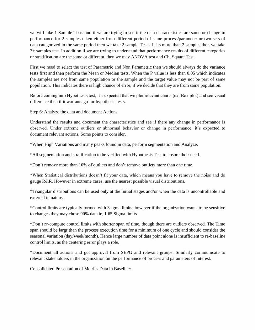
we will take 1 Sample Tests and if we are trying to see if the data characteristics are same or change in
performance for 2 samples taken either from different period of same process/parameter or two sets of
data categorized in the same period then we take 2 sample Tests. If its more than 2 samples then we take
3+ samples test. In addition if we are trying to understand that performance results of different categories
or stratification are the same or different, then we may ANOVA test and Chi Square Test.
First we need to select the test of Parametric and Non Parametric then we should always do the variance
tests first and then perform the Mean or Median tests. When the P value is less than 0.05 which indicates
the samples are not from same population or the sample and the target value may not be part of same
population. This indicates there is high chance of error, if we decide that they are from same population.
Before coming into Hypothesis test, it’s expected that we plot relevant charts (ex: Box plot) and see visual
difference then if it warrants go for hypothesis tests.
Step 6: Analyze the data and document Actions
Understand the results and document the characteristics and see if there any change in performance is
observed. Under extreme outliers or abnormal behavior or change in performance, it’s expected to
document relevant actions. Some points to consider,
*When High Variations and many peaks found in data, perform segmentation and Analyze.
*All segmentation and stratification to be verified with Hypothesis Test to ensure their need.
*Don’t remove more than 10% of outliers and don’t remove outliers more than one time.
*When Statistical distributions doesn’t fit your data, which means you have to remove the noise and do
gauge R&R. However in extreme cases, use the nearest possible visual distributions.
*Triangular distributions can be used only at the initial stages and/or when the data is uncontrollable and
external in nature.
*Control limits are typically formed with 3sigma limits, however if the organization wants to be sensitive
to changes they may chose 90% data ie, 1.65 Sigma limits.
*Don’t re-compute control limits with shorter span of time, though there are outliers observed. The Time
span should be largr than the process execution time for a minimum of one cycle and should consider the
seasonal variation (day/week/month). Hence large number of data point alone is insufficient to re-baseline
control limits, as the centering error plays a role.
*Document all actions and get approval from SEPG and relevant groups. Similarly communicate to
relevant stakeholders in the organization on the performance of process and parameters of Interest.
Consolidated Presentation of Metrics Data in Baseline:

PPB Sample Analysis:
Considering we have Defect Density and SLA Compliance as QPPOs (Y factor) and Few X factors like
Review Rate, etc the following could be the sample charts to be part of PPB.
Defect Density (QPPO – Y):
Histogram Depicts the Spread and Central Tendency of Defect Density, along with confidence Intervals.
P value refers to Normal Distribution.
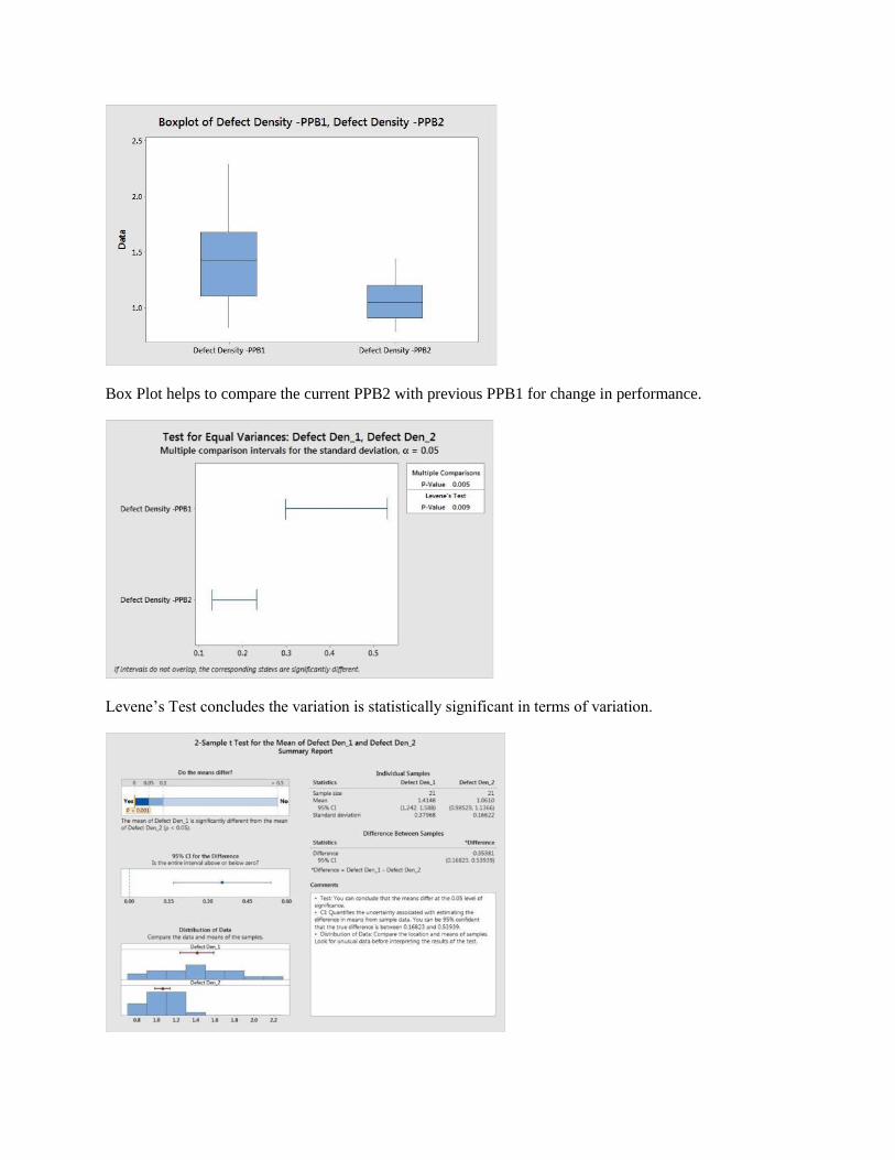
Box Plot helps to compare the current PPB2 with previous PPB1 for change in performance.
Levene’s Test concludes the variation is statistically significant in terms of variation.

2 Sample T Test confirms even the mean has difference which is statistically significant.
SLA Compliance (QPPO - Y):
Histogram shows the spread and central tendency, also the data is left skewed. P value indicates its not
normal distribution.
Distribution Identification shows the P value is high for Weibull distribution and AD value is acceptable.

Visible Performance Difference in Box Plot for current Period and Previous Period.
No difference in variance as per Levene’s Test (used for non-parametric conditions also, considering it
can tolerate certain level of distribution variation)
Mann-Whitney 2 sample Non Parametric test concludes the sample have different central tendency based
on median test.
Review Rate (Review Sub Process Measure – X factor) :

Histogram shows the distribution, Spread and Central Tendency. Greater than 0.05 P value indicates its
normal distribution. (Not all software unlike minitab may show this value, and you may need to conduct
separate normality test)
Control Chart shows many points as outlier against stability check rules and there is an upward trend
visible.

Visible Performance difference in Quarter 2 of 2015 in review rate, using Box Plot.
No Significant difference in Variance.

Mean of Review Rate in Q2 is different than of Q1 with statistical significance is proved using 2 sample
T Test.
Staged Control chart with new Control limits for Q2 period data is plotted in control chart.
Dot Plot Usage Sample:
Sample Dot Plot for Skill based Performance in Functional Design Complexity explains there high
increase in complexity based on Skill.
Remember not to use Control charts for plotting Y’s.
What We Covered:
Organizational Process Performance
SP1.4 Analyze Process Performance and Establish Process Performance Baselines

Define and Achieve Project Objectives and QPPOs
Defining Project Objectives and QPPO:
Project Objectives:
The Purpose of any project or Operation is to create/perform a work product/activity which delivers
values to the customer. In addition, how well the project/operation is performed in terms of cost, quality,
time and utilization, etc are critical to achieve Business Purpose of the Organization. On the other side
when an Organization has identified its Business Objectives to be achieved, it can only be achieved by
Projects/Operations meeting the value at Individual Level. Hence Project objectives has to be aligned
with Business Objectives, unless the client given objectives take priority or Current performance is much
better /lower than Organizations business objective or some of the Objectives has impact on other
identified objectives, etc. So every Project has to define their Project objectives in alignment with
Business Objectives. When the Project objective is not as per Business Objective, then it has to be
informed to senior management and approval has to be sought. This helps if many projects are getting
such situation, we may not achieve business objective, hence it has to be a conscious decision by
management.
The Project Objectives can be defined as SMART Objectives as defined in the Business Objective.
However usage of Confidence Level for a Project Objective depends on how frequently and how many
times the measure will be collected. When a measure like Profit Margin is computed in yearly basis we
may not be able to give confidence level, however the same when monthly profit margin or Operational
Effectiveness ratio is calculated its possible to have confidence level in definition of the measure.
Project QPPO:
In order to achieve the Project Objectives the Project level quality and process performance objectives has
to be identified. This can be taken from existing Organizational BO, QPPO relationship and can be
introduced at project level or when the project objective is client given then the logical QPPO should be
identified. The QPPO’s to be SMART in nature. New QPPO’s at project level is to establish statistical
relationship with Project Objectives, and for existing QPPO’s the Organizational level relationship can be
inherited if the conditions are valid. Based on the Project Objective and using existing relationships the
target for QPPO has to be set. For example if we want customer satisfaction more than 4.25 as index
(whereas organization BO had from 3.75 onwards) in a project level to maintain their reputation with
International client, the QPPO also has to have relevant value of Defect Density less than 1.0 Defects/Unit
(where Organizational QPPO may have less than 1.5 Defects/Unit). So Plan target of QPPO to achieve
the target given in Project Objectives. QPPO’s can have Confidence Level and also it should be like that
of getting values multiple times to use statistics. QPPO and Project Objective can’t be in same frequency
and at same time, then we don’t need QPPO to track, because Project Objective is directly available.
Hence QPPO frequency is higher than that of Project Objectives.
Both Project Objectives and QPPO’s to have Prioritization and this is useful when anyone of the
Objective is impacted while achieving the Other Objective. As given in the Project Objectives their
respective QPPO’s can have prioritization.

Sample Case
In our case of example here we are going to take one client given objectives and two existing Business
objectives for defining project objective and QPPO’s. The assumption is the project is having application
development and application maintenance activities both. The application maintenance activities provides
data periodically, however application development is more release and phase based. The major
enhancement falls under application development. Also we assume that customer satisfaction feedback is
largely dependent on quality of product delivered in this case. Considering the project is running for few
months by the time CMMI HM practices have been introduced for some of measures we know the current
performance, if so the following table will help in documenting the objectives.
Project Process Composition:
It’s nothing but selection of process/sub-process to be part of lifecycle to deliver a product/service by
knowing the processes ability to meet the Quality and Process Performance Objectives. Which means
either we have alternate processes for any given steps or we have factors which can influence process
depth of application, by knowing they would deliver different performance. To see this better, as a first
step let’s make the processes to be used in a deliver lifecycle to be available as process flow.

There are places where it’s possible for us to split the processes in to sub process, which has specific tasks
and clarity in outputs and roles involved. As a first step here we have identified the possible sub processes
and Processes. As a second step we need to understand which are the process/Sub Process where

alternates are available and where their performance are known. Select those sub process for composition.
In addition a simple Process Composition model, which is either based on existing PPM created at
Organizational level or prepared at project level using past data, can be used to perform what if analysis.
Which means, we select the sub-process/process based on their performance and potential contribution in
achieving the QPPO and/or we fix target for the sub process and processes within which they have to
perform, so that the QPPO can be achieved.
A case like defect density is the QPPO, whereas we have Review process with us can be considered with
technical review or inspection or walkthrough method. All three would offer different performances and
in past if we have used these methods their performance has to be part of Process Performance Baselines
and if not, it’s expected to baseline. Similarly there are other processes with alternate and their baselines
are taken. These baseline values are fed in to the Organizational PPM on defect density and what if
analysis is performed. To manually perform what if , you may need to select different methods
combination in each calculation using PPM, and reduce by 5%, 10%, 20% the values (basically that much
improvement) or just use different method and see if target from calculation is achieved.
Whereas using automated what if tools like Crystal ball optimizer can select the best possible
combination for us.
The model can provide the best possible combination of Processes for which it delivers the expected
defect density. When none of the existing processes are able to achieve the target, we may chose an
improved target for upto 20% at first level and run the model to see if the targets are meeting, still if we
don’t achieve the targets then we fix interim target of QPPO to ensure that practicality still wins.
Similarly when no alternate process is possible then level of application like number of reviews,
reviewers, processing time, usage of tools, repository usage, skill level of people, etc can be used to check
the process performance meeting targets, there by what if and process composition is achieved.
In our example its limited to defect density QPPO, the Crystal ball tool has suggested to use the
combination of inspection for review, custom architecture in design and combined feature and Risk

driven test methodology. On using this combination of processes, we will achieve defect density less than
1.38 Defects/size with 95% certainty.
Typically when we have multiple QPPO’s we have to have common PPM or Composite PPM, which is
useful in performing the trade-off between processes or even at QPPO level with process performance in
composing the processes for project.
Having selected the processes to be used in projects, the same has to reflect in the lifecycle.
Sub Process & attributes Selection for Monitoring and Controlling:
Along with Process Composition it’s important to see which of the sub process will be monitored using
statistical and quantitative techniques and be controlled. The Sub process which has shown high
sensitivity in PPM or in calculations, where past data is available and data collection is possible for
future, Logical correlation exist and its adequately frequent to perform in progress control. The sub
processes which meets most of the criteria is selected for monitoring and control.
For example Sensitivity chart for defect density reveals that Requirements Review, Design Complexity
and Functional Test Case preparation has higher influence on variance of Defect Density Results.
Where the count of Functional Test Case increase would negatively impact the defect density by reducing
it. On the other hands the Req-Review Rate and Design Complexity increase also increases the defect
density.
Based on this, further criteria for the sub process selection should be used to select sub process and their
attributes for statistical and quantitative monitoring,
Defect Density QPPO – Sub Process/process Selection with attributes

SLA Compliance QPPO – Sub Process/Process Selection with their Attributes,
Measures and their Analysis is given in table,
Which contains the analysis techniques to be used and further guidance to be elaboration in organizational
or project level guideline document on how to use the charts and interpret. The specification limits comes
from what if analysis which has to be used for Sub process/ Process monitoring and controlling, in order
to achieve the expected QPPO results.

Prediction using PPM and Planning Actions:
The Purpose of having a PPM is to understand proactively the ability to achieve the target and where
needed proactive actions are taken to ensure achievement of the target. At the beginning of a new Project
there may not be any PPM available with them, hence they can use the organizational PPM published for
their predictions. However its important to understand the PPM applicability in a given project
conditions. In some cases where dynamism is high the PPM can be prepared using the project data itself,
typically the Application Maintenance or any services based activities will fall mostly in to this category.
Hence collection of data at project level and then building a PPM might be required. Usage of
Organizational PPM to start with or Building own PPM both are dependent on context and they both are
acceptable. Once the PPM is selected the frequency at which we run is important for any proactive
monitoring and controlling. Based on type of work they can be run on milestone basis or on periodical
basis, however in both conditions its run at the beginning to understand what will be the achievement of
target. In addition the PPM has to use in the mid-course of the phase/period to accommodate if there is
any change in X factors or performance of Sub Process, etc.
Typically the PPM’s are either to predict the range of values which would occur or the certainty with
which the target will be achieved. Its not an forecasting model to predict the exact next value which
would occur. Based on the predicted value, its expected the actions are planned by the project team to
improve the target achievement or certainty. Typically it’s boiled down to controlling the X factors
(controllable) and Monitoring some of X factors (uncontrollable) and managing the characteristics of the
Project.
It’s important to track the predicted value with actual value, to ensure the values are not too different. The
usage of Mean Absolute Percentile Error (MAPE) is often helpful. For simplicity in conditions the
absolute deviation between the predicted and actual should not be more than a certain value (ex: 25%) , in
case if it exceeds, its important to study the PPM factors and if needed it has to recalibrated.
Recalibration of PPM can happen when a) Planned change in performance of Sub Process/Process b)
High Variation found in actual vs predicted, which on causal analysis found change in influence of X
factors c) Change in QPPO and/or business conditions d) X factors (when uncontrollable) are found to be
operating in values, beyond the current range of PPM boundaries.

At the Beginning of the PPM usage, we may not have X factors baselined at project level so we may the
Organizational Process performance baseline and run the PPM. However as we proceed with
phases/period and when we get the actuals we will keep replacing the values with actuals and where we
are yet to get the values (ex: the phase of functional test creation is yet to happen) we will use the
organizational values. So with these values we will be running the PPM and will see the target
achievement prediction.
We would change the X factors range only when it has a new performance baseline and its statistically
validated, however the influencing and uncontrollable X factors (like inflow of ticket) for which when
we get sufficient information we may alter the values in PPM and run.
Monitor performance of Selected Sub Process
The process/Sub Processes selected for monitoring has to be tracked for their performance. The
specification limits are typically derived from what if analysis. The trial control limits for any selected
sub process to be established with existing organization’s baseline of the sub process measure. We are
terming it as trial limit here not because it has less data points, but the process performance is taken from
organizational baseline. Once we get project level data we keep appending in the relevant charts to see if
the performance is same or its differing. When the performance is quite different than the Organizational
baseline (which you can understand by consistent outliers, stability test failures in control charts) its
important to baseline the projects’ process performance (with sufficient data , min >8 data point or >20
data point) and use that value. Hypothesis tests can help in finding the baseline value. When we have
more than 20 data points then the control limits derived from there is called natural limit.
The Processes selected for Monitoring will be collecting data as per the defined frequency, which is
typically event basis/periodical basis and keep plotting the data in the selected charts. Typically control
charts are used for statistical process control. Please see the Process Performance Baseline section to
understand more on control charts. The data are plotted with existing control limits and checked for
stability using stability tests (western electric rules). When data points fails in the stability tests then those
specific data points are studied to understand the cause and where its one time failure then actions are

initiated to prevent re-occurring. However if the points are more and following a pattern or unable to
assign any cause then its time to initiate a causal analysis process to do systematic changes to improve the
conditions.
Similarly when the control limits are within the Specification limits then we can classify them as Capable
Process. When they are overlapping on each other for some portion, then its better to do Cpk calculation
and check the process capability, along with declaring its not capable process. The process capability will
tell us how much we need to improve. A Cpk value more than 1.33 is considered as capable process.
When the process is not a capable process then also the causal analysis can be triggered.
When a control chart has very few outliers and they have assignable causes then they can be removed
from calculation of baseline, however we may choose to present them in control chart.
For example in our selected QPPO’s of Defect Density and SLA compliance the sub process measures
which we monitor are Requirements Review Rate and Analyze Time, and both of them are monitored
using control charts.

However as we do improvements to ensure process capability increases or due to unexpected changes in
business conditions, the data points may go out of control , In such conditions it’s expected to take a note
of such outliers and classify them as outliers due to planned change or not.

The purpose of control charts is to detect the changes quickly, however you may not decide to re-baseline
the control limits as soon as you find a shift, instead we may need to see sufficient data to understand the
variation/shift is significant and also for a minimum time period (so that the process shift is not because
of seasonal impact). However it’s important to track the process change as soon as we find the shifts.

Once we have sufficient data, we have to perform relevant hypothesis testing to see if the data suggests if
there is change in performance. When the hypothesis testing proves there is a change then the new
baseline control limits can be established.
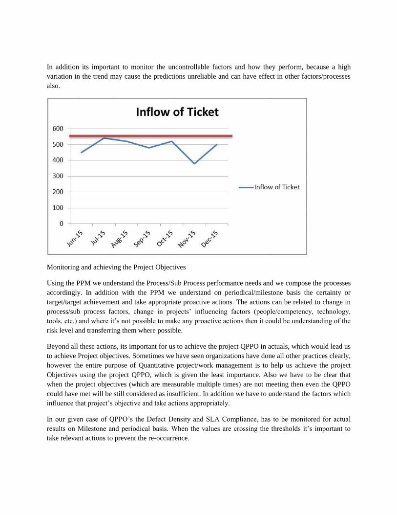
In addition its important to monitor the uncontrollable factors and how they perform, because a high
variation in the trend may cause the predictions unreliable and can have effect in other factors/processes
also.
Monitoring and achieving the Project Objectives
Using the PPM we understand the Process/Sub Process performance needs and we compose the processes
accordingly. In addition with the PPM we understand on periodical/milestone basis the certainty or
target/target achievement and take appropriate proactive actions. The actions can be related to change in
process/sub process factors, change in projects’ influencing factors (people/competency, technology,
tools, etc.) and where it’s not possible to make any proactive actions then it could be understanding of the
risk level and transferring them where possible.
Beyond all these actions, its important for us to achieve the project QPPO in actuals, which would lead us
to achieve Project objectives. Sometimes we have seen organizations have done all other practices clearly,
however the entire purpose of Quantitative project/work management is to help us achieve the project
Objectives using the project QPPO, which is given the least importance. Also we have to be clear that
when the project objectives (which are measurable multiple times) are not meeting then even the QPPO
could have met will be still considered as insufficient. In addition we have to understand the factors which
influence that project’s objective and take actions appropriately.
In our given case of QPPO’s the Defect Density and SLA Compliance, has to be monitored for actual
results on Milestone and periodical basis. When the values are crossing the thresholds it’s important to
take relevant actions to prevent the re-occurrence.

Perform Root Cause Analysis:
The Root cause analysis is performed as a tool to ensure that Sub-Process/Process maintains the stability
and be a capable process. In addition when the actual values of QPPO are not met, Root cause analysis
helps in identifying the cause to address it. The actions proposed by the root cause analysis may quickly
bring back the desired conditions or it can take long time also. It’s important to see when the actions are
not quick enough it impacts the QPPO achievement, which means the business results are impacted.
Hence the Project may seek additional actions, support and senior management drive to ensure they are
able to perform to meet the objectives. The actions taken which is considered part of Quantitative
management need not be elaborate and perform cost benefit and statistical tests, and it could be simpler

addressing of cause with actions. This is an extension of Project monitoring and control process’s
corrective action. We shouldn’t confuse it with Causal Analysis and Resolution.
What We Covered:
Quantitative Project/Work Management:
SG 1 Prepare for Quantitative Management
SP 1.1 Establish the Work Objectives
SP 1.2 Compose the Defined Process
SP 1.3 Select Subprocesses and Attributes
SP 1.4 Select Measures and Analytic Techniques
SG 2 Quantitatively Manage the Work
SP 2.1 Monitor the Performance of Selected Subprocesses
SP 2.2 Manage Work Performance
SP 2.3 Perform Root Cause Analysis
The simpler version of pictorial representation could be,


Causal Analysis in Project to achieve Results
Causal Analysis is a project level process which helps us to improve the performance of sub process
and/or QPPOs. The intention and the stage in which it’s applied determines whether is proactive causal
analysis and Reactive causal analysis. It’s important as an organization we have common guidance on
how and when causal analysis techniques can be triggered. Not every root cause analysis is a causal
analysis procedure. A root cause analysis could be qualitative or quantitative and it’s a technique to
identify the cause which is the root of problem, on the other hand a causal analysis is set of activities
formed to achieve desired results by identifying and addressing the causes on systematic manner in
addition using quantitative and statistical analysis support.
Causal Analysis can be done in the following conditions,
*Predicted QPPO has shortage in meeting Target QPPO (in terms of certainty or value)
*Critical Sub Process are not performing with stability
*Critical Sub Process are not having Capability
*Actual QPPO values are not meeting the Target QPPO
First bullet talks on “Proactive Causal Analysis” which is performed to ensure that project achieves the
results. The rest of the bullets talk on “Reactive Causal Analysis” to ensure the performance is improved
from current status. In addition some cases the causal analysis can be triggered to understand the actions
which are behind improvement which are noticed, but not planned earlier.
Team Formation:
Considering it’s a technique predominately expected (applying in other functions or group level can be on
need basis) to be used in project level, it’s expected to have causal analysis team with identified people.
The people can represent various roles in the project team and they understand the project conditions
well. It’s also expected that they have undergone training on causal analysis techniques as this will help in
achieving better results. The team has to meet on periodical basis to understand conditions, find triggers
and monitor the current causal analysis actions. In addition on need basis/milestone basis they can meet to
work on causal analysis. The causal analysis team can have process experts also, so that the process point
of view causes can be addressed appropriately.
Selection of Outcomes:
As discussed in the trigger the QPPO, Process performance values, X factors are typical outcomes which
will be considered in causal analysis. In some cases, where improvement of Sub Process/Process
performance will be the outcome to be improved, however it will have positive impact on the QPPO and
it might be linked with the Process performance models. So the outcome selected (if its process factor)
will have improvement target which is relevant to final QPPO improvement. As an approach a project
may start using this formal analysis on selected QPPO and sub process and later expand it to all
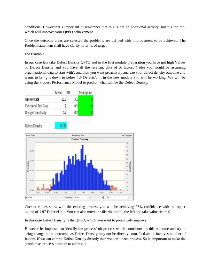
conditions. However it’s important to remember that this is not an additional activity, but it’s the tool
which will improve your QPPO achievement.
Once the outcome areas are selected the problems are defined with improvement to be achieved. The
Problem statement shall have clarity in terms of target.
For Example
In our case lets take Defect Density QPPO and in the first module preparation you have got high Values
of Defect Density and you have all the relevant data of X factors ( else you would be assuming
organizational data to start with), and then you want proactively analyze your defect density outcome and
wants to bring it down to below 1.5 Defects/unit in the new module you will be working. We will be
using the Process Performance Model to predict, what will be the Defect Density.
Current values show with the existing process you will be achieving 95% confidence with the upper
bound of 1.97 Defect/Unit. You can also move the distribution to the left and take values from 0.
In this case Defect Density is the QPPO, which you want to proactively improve.
However its important to identify the process/sub process which contributes to this outcome and try to
bring change in the outcome, as Defect Density may not be directly controlled and it involves number of
factors. If we can control Defect Density directly then we don’t need process. So its important to make the
problem as process problem to address it.

In this case, we assume that Sensitivity Analysis revealed that High Requirements Review Rate as part of
Review Process is a contributing factor in our Process Performance Model. In such case the Requirements
Review Process and the Review Rate is the controllable factor which we need to monitor and control.
As given in the PPM, the mean is 10.9 and Standard deviation is 3.1, we assume the data is normal (you
have to do normality test).
With what value of Review Rate we will be getting 95% certainty of Defect Density at 1.5 Defects/unit,
we need find using what if Analysis.
In our case, for example Review Rate Mean is 6 and maintaining standard deviation, we will be getting
the Defect Density of 1.5 with 95% certainty (keeping functional test cases, functional design complexity
as same). This is an approximate Reduction of 40% on the Review Rate (pages/hour).
Categorize and Perform Root Cause Analysis:
Many a times, it may be more useful to split the outcome in to different category and then perform
analysis. This is useful first level analysis and it reduces the effort which we need to put on root cause
analysis and reduces complexity. How to come out with new categorization when we don’t have such
categorization and data in the format is the typical question. When you don’t have the data most of the
time either sampling or reengineering data with categorization for recent period data might be required.
The following table can be used to think on categorizing data,

Once we do first level categorization and arrange our existing data in them, it would be easier to study on
variation which is happening.
Then we can select specific category of reason/group to understand the root causes behind them in detail
with the Causal Analysis team and with selected individuals who are experts in the area. The root causes
can be again quantified to see how important it is.
The example given in our case Defect Density and high review rate, we will directly perform the Root
cause analysis to find different root causes,

The RCA reveals few causes are key reasons for high review rate, so further we collect the occurrences
Here just consider the Number of Occurrences for the period of Jun 15 for all the 4 categories and its clear
that estimation and checklist are the 2 key reasons (you can use pareto chart).
Identify and Implement Actions:
Knowing the root causes and their level of influences on the Performance, we can work on which are the
root causes we want to remove /reduce the occurrence. The action items can be identified against them.
In addition the actions can be many and not all the actions can be fruitful in delivering the results. Hence

its recommended to use cost benefit Analysis or any equivalent technique to see if the actions are useful.
There will be no meaning in spending huge cost in improving the performance, where the Returns are
lesser than it. Hence its expected to such analysis and then select the actions for implementation.
Usage of PPM is recommended in this case also.
In our case where we already selected the causes the action selection could be listing actions and perform
cost benefit analysis.
Here we selected actions where the estimation sheets to have standard estimation value for Reviews and
adequate effort to be allocated for reviews.
We have also tracked it with relevant monitoring and closed them in sep 15.
Evaluating the Results:
The actions should have resulted in reducing the causes, so in our case if you have seen earlier chart on
occurrences for the 4 causes, in sep 15 the values of low estimation has become zero. Hence the actions
had impact on arresting the root cause. The next step is to see, whether this condition has helped in
overall process performance which we targeted, Hence we have to do before and after comparison of the
process performance after actions are completed.
Once we understand there is change in performance, then it has to be statically proven that its significant
in achieving the target. Once its proved the control limits/new baseline limits can be achieved. The same
can be further used in Process performance models. The cases where the Outcome selected is not limited

to stability of Sub process/ Process, its important to see how the results are impacting the QPPO. Hence
using the revised control limits/distribution co-ordinates the certainty or target prediction can be done. If
the results are not adequate, the relevant actions can be taken.
You can see there is clear drop in estimation causes.
Box Plot shows the mean is significantly reduced, also there is slight change in variance, but doesn’t look
signification. Hence we will do Hypothesis test for mean.

P value is less than 0.05 so we can interpret the performance is significantly changed. So we will revise
the control limits with new data after action completion.
With the new values of Review Rate achieved (which approximately equal to the targeted value) , we will
what is the actual value of Defect Density in the same period.

The actual Defect Density is lesser than 1.5.
However its important to see what will happen in the future with current variations, so we use the process
performance model with the revised Review rate and other factors as it is and we will run it.
We have got 95% certainty at Defect Density 1.5 Defects/Unit in this case, so we have achieved the
results as expected. So we can claim the causal analysis is effective and successful. However in some
cases, you may not achieve the exact values as expected, however its still fine.
Example on SLA Compliance:
Assuming we have SLA compliance to improved and the current capability of the X factor Analyze Effort
is less as its performing at Mean 103 and SD 26 and we had to make improvement 30% in mean and 60%
in SD to achieve an improvement 5% in SLA compliance is the outcome selected. The following is the
example charts to see how we might go on addressing them,

We study the application wise analyze effort to understand if there is variation (refer the table on
categorizing) and we found application A is taking more time.
Further Root cause analysis reveals inadequate information for tickets and dependencies create more
effort as application has similar functionalities in few areas. We assume the occurrences are 15 times in
this category.
Actions are evaluated and the incident tool is added with more details and categorization of incidents for
the tickets.

The actions are completed on time.
Also we assume the occurrence have reduced to zero and further it has impact in entire set of Application
A tickets, so we have to study the performance of Analyze effort for application A. (from below chart its
clear there is significant improvement as there is no overlapping region between groups)
Then we will study change in performance in overall analyze effort,

Visually its shows there is difference in mean and in variance,

We can see Hypothesis for variance and Mean shows there is significant change. Hence we will revise the
control limits,
If we want to study the impact on SLA compliance, we can still use the PPM and run to see the certainty
using the new values of Analyze Time.
Causal Analysis Repository and Trigger for Improvements:
The Causal Analysis data has to be submitted to the Software Engineering Process Group to show how
the process changes and root cause addressing has resulted in improvement or non improvement. Success
and failure both are important to study and understand how the process components have behaved with
variation on applications and yielded results. These have to be reviewed and organized as respository by

SEPG. They may chose to categorize them in any particular format , which will be easier for projects to
select for their case (ex: QPPO wise or Sub process wise or project type wise or technology wise, etc).
Simply uploading a presentation may not be really useful in a repository and hence its recommended to
improve the Organization of repository. In addition good causal analysis are a source for identifying
improvements which can be deployed across the organization. For example in this case, effort
standardization in the template for review to be deployed across the organization. The smaller changes
shall be part of SEPG regular Organizational deployment activities and need not be part of Organizational
Innovation ideas.
Causal Analysis and Organizational Innovation differs by the reason they are performed as the first one in
is mostly to a specific case and localized improvements, and the second one is larger area and covers most
of the organizational part. Causal Analysis is a key source for improvement Ideas in the Organizations ,
however it may not be on the reverse.
What We Covered,
Causal Analysis and Resolution
SG 1 Determine Causes of Selected Outcomes
SP 1.1 Select Outcomes for Analysis
SP 1.2 Analyze Causes
SG 2 Address Causes of Selected Outcomes
SP 2.1 Implement Action Proposals
SP 2.2 Evaluate the Effect of Implemented Actions
SP 2.3 Record Causal Analysis Data


Driving the Innovation/Improvements to achieve Business Results
Driving Improvements to achieve Business Objectives:
As an Organization we have identified the Business Objectives to be achieved in the near future and have
organized our projects to align themselves towards these objectives. The projects are direct contributors to
achieve the business objectives as they produce results to be achieved and support functions are aligned to
ensure that projects could achieve these targets. In such scenario, we will be monitoring the performance
of projects results from the point of view of achieving business objectives on periodical basis. This could
be quarterly basis for an annual business objectives or half yearly for Business objectives targeted
biyearly basis and so on. The regular understanding on business performance with the help of actual
business results and how the Quality and process performance objectives have been performing, helps the
SEPG and Senior management to identify improvements needed in the Organization’s Process
performance. Typically set of process initiatives which are new innovation or improvements could be
identified regularly, which would overcome the challenges and boost the business results achievement
would be part of their charter. Thus such initiatives helps to improve QPPO achievements and there by
Business Objectives achievement. These initiatives are tracked to deployment, so that the entire
organization (as applicable) gets the benefit in terms of improvement from current state. Hence its like
Organizational Stock taking on performance versus target and bridging the gap or moving above limits
using process improvement initiatives on ongoing basis.
Revising and Updating Business Objectives:
The SMART Business Objectives set in the Organization on a given time, might have been achieved in a
period of time or the Organization would have understood that the targets are too wide or high or low so
they may want to revise them. In addition the Business Objectives could have been no longer valid when
the business scenario changes. Hence its important to periodically monitor the Business Objectives
suitability and the targets suitability, if needed they have to be revised. As we revise the Business
Objective the QPPO which are aligned with that will also to be revised. In addition the relationship
established between the QPPO and Business Objectives could differ in a given time period in certain
contexts, hence its important to see the relationships are still valid in the similar level. Also within
Business objectives and QPPO also the priority may have shifted, so the prioritization to be checked on
regular basis. The Senior management team along with SEPG can do meetings on periodical basis to
verify the performance and take necessary actions.
Analyzing the Performance Results and Identify Potential areas of Improvement
On periodical interval the Business and Process results to be analyzed using relevant quantitative and
statistical techniques. The Shortage in Business performance results to be studied and the actions to be
identified, in addition any potential area where improvement initiatives can be run to be also identified.
Typically along with Process Performance Baseline preparation the Business Objectives results
achievement for the period to baselined and using the values of BO and QPPO actuals, we can compare
and understand the improvements in results. As the Business Objectives could be for a given time period
the organization may have interim targets identified for periods, so on the given period what should have

been the results which will help your organization to achieve the Business objective on annual/biyearly or
for a give time could be understood. So its expected that the results are compared with Interim targets in
the interim periods to make the comparison meaningful. Where there are shortages they have to be noted
and the areas relevant to that BO/QPPO can be the potential areas for improvement Initiatives. These
areas can be discussed with senior management by SEPG and actions can be planned. In the Initial
periods , we may not be clear on what type of initiatives on how much they would benefit in the given
area, however as the initiatives go to the next level, we will be having adequate information on how much
these initiatives will contribute.
Many a times organizations ask, how many improvement initiatives are needed for CMMI High maturity.
The answer is CMMI don’t decide it, but your Business Goals decide, your performance decides it.
CMMI Is a performance based process Improvement model , when it comes to high maturity. Here the
entire idea of having Improvements/innovation is to find your shortages in performance or your
performance improvement needs and have that many initiatives. From an appraisal point of view it could
be even one is sufficient, but is that what your organization need is, that you have to decide.
A table given below could be the way these analysis and performance related process improvement areas
could be identified,
Techno Process Innovation Group and its functions:
The Organizations Operating at maturity level 5 of CMMI to have a group like Techno Process
Innovation group, which can understand the technical and process needs and able to innovate or improve
the processes. The aim should be to continuously improve the performance using the modern technologies
and process designs. The group can comprise of technological experts and process experts and can be
extended arm of SEPG or Separate function as per the need of the Organization. The group shall meet on
regular intervals to find new suggestions and opportunities to innovate or bring best practices from
relevant industries or to experiment a projects success factor at organizational level, etc.

Typically in software industry the problems are very close to Time, Cost and Quality factors and our
innovations/improvements are also focused to them. Innovation is achieving beneficial results in an
unexpected way and its significantly different from current way of performing to get the results. From
product point of view Innovation can be significant addition/modification of functionalities in product
which achieves beneficial results. Whereas improvements are incremental in nature to the current way of
performance and it could be addition/modification to the current functionalities in product. The following
chart helps in identifying improvements to the current performance factors.
Collect improvement Suggestions and select appropriate Suggestions:
Improvement suggestions should be collected in an organization on periodical basis. The organization
shall have mechanism to collect and analyze them on regular basis, which means a group like Techno
Process group looks at each suggestion and make decision to go ahead or not. The suggestions can come
from,
*Employee Suggestion/Feedback Box/online form
*Appraisal/Audit Reports
*Process/Technological Workshops
*Customer Feedback/Survey
*Improvements survey
*Management Review sessions
*Brainstorming meetings of Techno Process Group
*Others

These suggestions to be captured in a particular format to ensure the relevant information are there. The
details on person who raises these suggestions, the impact on BO/QPPO and its relevance, expected
benefits and further additional details to be captured in the Process Improvement suggestion log/tool.
Similarly each suggestion to be evaluated for probable cost, time it will take and contextual relevance and
BO/QPPO Impact. When there is benefit assumed then it has to be selected for next level analysis or for
further deployment. Not all the suggestions may be relevant to BO/QPPO but it can be relevant to people
and working environment ,etc in such case also the improvement has to be considered for deployment,
however the rigor of application of statistics will not be there, but can have minimal quantitative analysis.
The selected improvements has to validated for further deployment, this could be achieved by having
conference room simulation, prototype, expert reviews and piloting, etc. Many organizations chooses
piloting as default technique for all improvements, which is not necessary. For example the improvements
comes from causal analysis of a recent project which has benefitted in achieving its project level
objectives, then do we still need piloting or if the improvement is on developing a tool for addressing
some of the process needs then is it possible to have piloting, the answer is no. The model never describes
piloting as the only methodology for validation, however its very common to see the organizations and
certified individuals push for piloting as safe mechanism to validate improvement suggestion.
In our case of SLA Compliance (QPPO), the analyze effort is on higher side and it can be reduced using
the improvement of KEDB (Known Error DataBase) implementation in the Organization and relevant
tool is also recommended in the suggestion. A initial study and data collected from different past
engagements reveal that there is a negative correlation exists.

However the Organization is not clear whether it will work well on other complex technologies and to
understand the benefits clearly they decided to pilot.
A pilot plan can be something like this (contents are detailed ones)
Pilot Plan:
Objective:
To Improve Analyze Time by 40% by using KEDB application, thereby Improving SLA Compliance by
10%
Pilot Applicable:
Project A and B to be the Pilot Projects
Pilot Schedule:
*Task 1 – starts on 10 Mar 15 and Ends on 18 Mar 15- XBS Responsible
*Task 2- starts on 21 Mar 15 and Ends on 28 Mar 15- ASS Responsible
*Task 3 - starts on 01 apr 15 and Ends on 28 Apr 15- DSB Responsible
*Others……
*Evaluation of Pilot – Starts on 01 May 15 and Ends on 10 May 15 – XBS Responsible
Stakeholders:
Project Teams, Senior Management, and Improvement team
Provide complete Involvement matrix
Environment Needs:

….
Pilot Success Criteria:
*All Projects Implement KEDB
*Minimum of 30% Reduction in Analyze Effort atleast in Repetitive incidents
*Minimum of 5% Potential Improvement in SLA Compliance using PPM (actual for the given month is
better)
Pilot Exit Criteria:
*Completion of All tasks
*Projects not able to progress to complete the tasks
Measurements:
Time and Cost Spent on Piloting and Impacted Results as per Success Criteria will be measured.
Others:
…………..
After piloting the KEDB for the given period the Organization realizes certain improvements,
Analyze Time has reduced significantly

Similarly the KEDB application is stable in projects,
There is an improvement in the SLA Compliance with Piloting of KEDB

Further the pilot results are published,
*Improvement seen in Analyze Effort – mean Shifted from 100 to 60 (approximate 40% improvement)
and SD remains same
*Potential Improvement in SLA seen by 5% Improvement, which crosses the Penalty value of 80%
Compliance.
*Its Practical to implement and High Support Received from Project Team
Improvement in Moral is visible in Project
*Cost & Benefit:
Pilot Effort for KEDB Implementation = Person Days * Cost Per Day => 5* 120 =600$
Benefit: Penalty on atleast 5% of tickets on SLA Compliance is reduced = % improvement*
No.of ticket crossing SLA* Penalty Value=> 0.05*50*500=1250$
Reduction in Analyze Effort, there by Team works on Enhancements = Person Days * Cost Per
Day* People in Project=> 0.09* 120*50= 540
Total Benefit in Month= (1250+540)-600=1190$
*Recommended for Deployment based on Time to Implement, Benefits Realized and practicality in
application.
The Report is submitted for approval with senior management for further steps in to deploying them
across the organization (as applicable). Once the approval is attained then the improvement suggestion is
taken for deployment.
Where pilot results are not encouraging the Improvement suggestion can be dropped with a clarity that
it’s a failed pilot program and it will not be taken for deployment.
Deploying Process improvements and evaluating them:

Deployment needs preparation and strategy before get on to the field for application of improvement
solutions. The improvement solution should be clearly drafted, where applicable the tools to be made
available or created, relevant manuals to be ready, Process changes submitted to SEPG for release in
QMS, Training the relevant Stakeholders, etc to be prepared before deployment. The deployment strategy
could be of identification of phases in deployment, change management needs, criticality and
prioritization of deployment, entry and exit criteria for deployment, stakeholder involvement, managing
budget for deployment, etc
Typically a deployment plan is prepared once the initial preparations are done with the improvement
solution,
Deployment Plan:
Deployment Team:
SEPG
Improvement Team
Scope of Deployment:
All Application Maintenance Engagements which have SLA as QPPO
Deployment Approach:
Inventory of AM Engagements suited to apply the improvement
Communicate usage of KEDB to the selected AM Engagements
QMS Update
QMS is to be updated with generic KEDB template if applicable
Tracking Mechanism:
Bi-weekly checks
Monthly Monitoring of values
Deployment Schedule:
*Current Baseline and Individual Planning for Projects – starts on 10 Jun 15 and Ends on 18 Jun
15- XBS Responsible
*Training Teams- starts on 21 Jun 15 and Ends on 28 Jun 15- ASS Responsible
*Handholding usage of KEDB - starts on 01 Jul 15 and Ends on 28 Sep 15- DSB Responsible
*Others……
*Evaluation of Deployment – Starts on 01 Nov 15 and Ends on 20 Nov 15 – XBS Responsible
Deployment Exit & Success Criteria:

*Completion of All tasks
*Completion of Deployment Schedule
*Projects not able to progress to complete the tasks
*Success Criteria – Atleast in 80% of projects Analyze Effort reduced by 30% and SLA Compliance
improved by 5% or more
Stakeholders Involvement:
…..
Measurements:
Time and Cost Spent on Deployment and Impacted Results as per Initiative will be measured.
Risks and Strategy to Encounter:
……..
Others:
……
The deployment to be performed as per the plan, in addition a deployment of process improvement shall
be a time boxed process/technical handholding activity with concentrated effort. Once the tasks are
completed the organization should close the deployment and leave it to regular support. Which means the
Quality management system and regular organizational structure & system is now capable in handling the
solutions. In other words, they are institutionalized and no need of separate effort through deployment to
handhold. Once the deployment is performed the deployment results to be statistically validated,

KEDB implementation in control (the outlier are not removed in this case)
The deployment results on Analyze Time is similar to those of piloted projects and its supported by the
relevant statistical tests (box plot, Hypothesis test – not included here)
Similarly we could see improvement in performance on SLA Compliance in the pilot and deployed
projects.
Revising Process Performance Model:
Once there is change observed in X factors performance baseline then immediately its important to
understand that no longer the process performance model with past performance may valid. So the model
can be reconstructed with new values in some cases (static models) or just re-caliberation of model in
some cases (dynamic models).
So in a similar case on Defect Density (QPPO) where the functional test case numbers are pretty low and
new test framework standards are introduced by the organization to improve the quality and quantity of

functional test cases as improvement suggestions the following are the typical charts which may be
established with relevant statistical tools application.
(Functional Test case count increase – outlier not removed with relevant reasons)

Improvement observed in Defect Density by reduction.
Here the factor of influencing is the usage of test framework on all the modules, which will be discrete in
nature (Yes/No) the results of their impact with functional test case count can be studied with ANOVA.
Once the deployments are evaluated they are closed with lessons learnt and completion report. The
reports to be submitted to SEPG for future reference and also can be published with organizational
repository.
Again don’t forget to link that this an organizational Performance management tool, so all the results are
evaluated to see it makes the life easier for your organization to achieve the business objectives. Hence
the real success of an improvement remains in achieving the business results.
What we have covered:
SG 1 Manage Business Performance
SP 1.1 Maintain Business Objectives
SP 1.2 Analyze Process Performance Data
SP 1.3 Identify Potential Areas for Improvement
SG 2 Select Improvements
SP 2.1 Elicit Suggested Improvements
SP 2.2 Analyze Suggested Improvements
SP 2.3 Validate Improvements
SP 2.4 Select and Implement Improvements for Deployment
SG 3 Deploy Improvements
SP 3.1 Plan the Deployment
SP 3.2 Manage the Deployment
SP 3.3 Evaluate Improvement Effects

Succeeding in High Maturity Appraisals
Implementation Readiness for Appraisal:
As we progress in implementing CMMI High maturity practices its important to check the
implementation at periodical intervals. The preparation towards Scampi A appraisal requires a clear
roadmap with periodic appraisal/spot checks to understand the implementation of CMMI practices and
where required correct the understanding. The coverage of these checks (or facilitated by consultants or
review by HMLA) may start from up to L3 to L4 and then to L5 process areas. In addition all the projects
shall have their own mapping of CMMI HM implementation to check how far they are in following the
practices, alternatively detailed audit or periodical reviews in these projects may be a tool for
implementation checks. The evolution may take anywhere from 20 months to 36 months or longer from a
maturity level 3 organization to maturity level 5. For organizations going for reappraisal which is
consistently following the CMMI practices can increase the internal appraisal and checks in the last one
year.
Selection of HMLA:
The High Maturity Lead Appraiser selection is an important area for successful Appraisal. You will have
advantage when, the Appraiser have prior experience in appraisal in the business to be appraised, the
appraiser has performed prior ML5 Appraisal successfully, the appraiser has right number of clients with
him to make availability for your appraisal. Considering there is definite chance of interpretation variance
between appraisers and between consultants and within them, it always better to have HMLA identified
earlier and engage him/her in early reviews to get their views. It has to be done at least 8 to 10 months
before.
Planning SCAMPI A:
It’s important to define the Organizational unit with scope of CMMI Implementation. The business areas
and locations from which delivery/services happen which are part of the Organization to be listed. The
number of people working on delivery and support functions and their roles to be listed. Similarly
applicable CMMI process areas and optional Process Areas inclusion and exclusion to be clearly stated.
The Organization may identify the sampling factors along with the HMLA guidance early to understand
how their appraisal would be and also to provide relevant information while making the appraisal plan
document.
Typical sampling factors include, Location wise, Customer wise, Size, organizational Structure, Type of
work difference in terms of delivery and QMS implementation. The HMLA may be able to find the sub
groups with these factors or may be more relevant factors can be used in discussion with your
Organization. Knowledge in SCAMPI Method Definition Document will help you to understand on how
sampling in final appraisal will work.
Typically 5 to 6 month before itself these information can be generated.
ATM Selection:

The Appraisal Team Members in High maturity appraisals should have adequate experience in lifecycle
which is appraised and understanding on process (Please refer SCAMPI MDD for requirements). In
addition there shall not be any conflict of interest of their ATM role with the role performed in the
Organizational unit. Similarly many reporting relationships within the ATM group is also to be avoided.
Under unavoidable conditions, it has to be reported in appraisal plan and appropriate actions to be taken
as per HMLA Guidelines. The ATMs should be trained in CMMI Introduction official training for 3 days
and they have to be trained as Appraisal method (ATM training ) by the HMLA for 2 days (unless they
are already trained). In addition people who will be appraising the high maturity process areas shall have
adequate understanding on statistical and quantitative concepts.
Pre-Appraisal:
A Pre-Appraisal or SCAMPI B appraisal can be conducted atleast 4 to 5 months before to ensure the way
high maturity practices have been implemented is appropriate , if not we have time to correct our
understanding and adjust. The Pre-appraisal should have atleast 50 to 60% of projects to be taken in to
final SCAMPI A appraisal.
Managed Discovery Appraisals:
Its common to see many a times managed discovery methods are used in SCAMPI Appraisals, which
reduces the PIID development time, instead we have to only give a catalog and repository of artifacts as
input to appraisal. Any additional documents will be sought based on interviews and document review.
SCAMPI A Appraisals:
To start with the Sponsor to be minimum available on Starting and final day of appraisal, in addition on
finalizing the documents, etc. The Site coordinator role plays vital role in ensuring the timeline of
interviews , facilities needed, etc are arranged. The interviews will be conducted as planned with different
roles from projects and with functions. The documents are corroborated with oral affirmation to see the
implementation. The draft findings are generated by the appraisal team and presented to the participants
in appraisal, based on the feedback and further understanding the final findings are generated and
reported. The Sponsor may choose to make the results public or not, so the announcement of your
appraisal will be performed based on the consent of Sponsor.
The announced reports will be submitted to the CMMI Institute and based on their final check, they
would publish the reports in PARS ( if opted by the Appraised Organization).
Combined Appraisals:
CMMI Dev and SVC ML5 or ML4 can be combined appraisals if the organization, wish to select that
way based on their implementation. The benefit we would be getting is reduced training effort for
appraisal team members and reduced interview timings for project members. The other factors like
document study and rating of practices/goals/PA will remain same and may not lead to any less effort.
However it helps when the projects have Services and development components together.
Extension Appraisals:

In SCAMPI A the recent addition is extension appraisals and these are very helpful to ensure the failed
goals of a process areas and impacted process areas alone can be re-appraised if the HMLA feels its
adequate. This eliminates the cost of the overall SCAMPI A conduction, when the first SCAMPI A has
shown there is limited goals are impacted because of weakness and could be corrected in a given period
of time, which is not more than few months ( Refer SCAMPI A v1.3 b MDD). However these appraisals
can’t be like iterative appraisals forever and can only be done once.

Reference, Links and Contributors
This book can be studied along with the following other books for getting high expertise on Software
Quality assurance and in CMMI Model.
*CMMI Implementation Guide
*Jumpstart to Software Quality Assurance
Thanks to the following people for their contribution in this Journey:
Thirumal Shunmugaraj
Harshad Bile
Koel Bhattacharya
Leena Sagar
Mitta Rout
Rahul Singh
Snehal Pardhe
Sonali Khopkar
Sunil Shirurkar
Viloo Shastri


