
Using Nonnegative Matrix and TensorFactorizations for Email Surveillance
Semi-Plenary Session IX, EURO XXII, Prague, CR
Michael W. Berry, Murray Browne, and Brett W. Bader
University of Tennessee and Sandia National Laboratories
July 10, 2007
1 / 51
Collaborators
◮ Pau’l Pauca, Bob Plemmons (Wake Forest)
◮ Amy Langville (College of Charleston)
◮ David Skillicorn, Parambir Keila (Queens U.)
◮ Stratis Gallopoulos, Ioannis Antonellis (U. Patras)
2 / 51
Non-Negative Matrix Factorization (NMF)
Enron Background
Electronic Mail Surveillance
Discussion Tracking via PARAFAC/Tensor Factorization
Conclusions and References
3 / 51
NMF Origins
◮ NMF (Non-negative Matrix Factorization) can be used toapproximate high-dimensional data having non-negativecomponents.
◮ Lee and Seung (1999) demonstrated its use as a sum-by-parts
representation of image data in order to both identify andclassify image features.
◮ [Xu et al., 2003] demonstrated how NMF-based indexingcould outperform SVD-based Latent Semantic Indexing (LSI)for some information retrieval tasks.
4 / 51

NMF for Image Processing
SVD
W H
A i
i
U ViΣ
Sparse NMF verses Dense SVD Bases; Lee and Seung (1999)
5 / 51
NMF for Text Mining (Medlars)
0 1 2 3 4
10
9
8
7
6
5
4
3
2
1 ventricularaorticseptalleftdefectregurgitationventriclevalvecardiacpressure
Highest Weighted Terms in Basis Vector W*1
weight
term
0 0.5 1 1.5 2 2.5
10
9
8
7
6
5
4
3
2
1 oxygenflowpressurebloodcerebralhypothermiafluidvenousarterialperfusion
Highest Weighted Terms in Basis Vector W*2
weight
term
0 1 2 3 4
10
9
8
7
6
5
4
3
2
1 childrenchildautisticspeechgroupearlyvisualanxietyemotionalautism
Highest Weighted Terms in Basis Vector W*5
weight
term
0 0.5 1 1.5 2 2.5
10
9
8
7
6
5
4
3
2
1 kidneymarrowdnacellsnephrectomyunilaterallymphocytesbonethymidinerats
Highest Weighted Terms in Basis Vector W*6
weight
term
Interpretable NMF feature vectors; Langville et al. (2006)
6 / 51
Derivation
◮ Given an m × n term-by-message (sparse) matrix X .
◮ Compute two reduced-dim. matrices W ,H so that X ≃WH;W is m × r and H is r × n, with r ≪ n.
◮ Optimization problem:
minW ,H‖X −WH‖2F ,
subject to Wij ≥ 0 and Hij ≥ 0, ∀i , j .◮ General approach: construct initial estimates for W and H
and then improve them via alternating iterations.
7 / 51
Minimization Challenges
Local Minima
Non-convexity of functional f (W ,H) = 12‖X −WH‖2F in both W
and H
Non-unique Solutions
WDD−1H is non-negative for any non-negative (and invertible) D
8 / 51

Alternative Formulations [Berry et al., 2007]
NMF Formulations
Lee and Seung (2001)Information theoretic formulation based on Kullback-Leiblerdivergence of X from WH
Guillamet, Bressan, and Vitria (2001)Diagonal weight matrix Q used (XQ ≈WHQ) to compensate forfeature redundancy (columns of W )
Wang, Jiar, Hu, and Turk (2004)Constraint-based formulation using Fisher linear discriminantanalysis to improve extraction of spatially localized features
Other Cost Function FormulationsHamza and Brady (2006), Dhillon and Sra (2005), Cichocki,Zdunek, and Amari (2006)
9 / 51
Multiplicative Method (MM)
◮ Multiplicative update rules for W and H (Lee and Seung,1999):
1. Initialize W and H with non-negative values, and scale thecolumns of W to unit norm.
2. Iterate for each c , j , and i until convergence or after kiterations:
2.1 Hcj ← Hcj(W T
X )cj
(W TWH)cj + ǫ
2.2 Wic ←Wic(XH
T )ic
(WHHT )ic + ǫ
2.3 Scale the columns of W to unit norm.
◮ Setting ǫ = 10−9 will suffice [Shahnaz et al., 2006].
10 / 51
Normalization, Complexity, and Convergence
◮ Important to normalize X initially and the basis matrix W ateach iteration.
◮ When optimizing on a unit hypersphere, the column (orfeature) vectors of W , denoted by Wk , are effectively mappedto the surface of the hypersphere by repeated normalization.
◮ MM implementation of NMF requires O(rmn) operations periteration; Lee and Seung (1999) proved that ‖X −WH‖2F ismonotonically non-increasing with MM.
◮ From a nonlinear optimization perspective, MM/NMF can beconsidered a diagonally-scaled gradient descent method.
11 / 51
Lee and Seung MM Convergence
Definitive Convergence?
When the MM algorithm converges to a limit point in the interiorof the feasible region, the point is a stationary point. Thestationary point may or may not be a local minimum. If thelimit point lies on the boundary of the feasible region, one cannotdetermine its stationarity [Berry et al., 2007].
Recent Modifications to Lee and Seung MM
Gonzalez and Zhang (2005) accelerated convergence somewhatbut stationarity issue remains.
Lin (2005) modified the algorithm to guarantee convergence to astationary point.
Dhillon and Sra (2005) derived update rules that incorporateweights for the importance of certain features of the approximation.
12 / 51
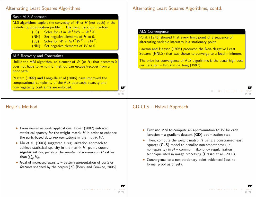
Alternating Least Squares Algorithms
Basic ALS Approach
ALS algorithms exploit the convexity of W or H (not both) in theunderlying optimization problem. The basic iteration involves
(LS) Solve for H in W TWH = W TX .(NN) Set negative elements of H to 0.(LS) Solve for W in HHTW T = HXT .(NN) Set negative elements of W to 0.
ALS Recovery and Constraints
Unlike the MM algorithm, an element of W (or H) that becomes 0does not have to remain 0; method can escape/recover from apoor path.
Paatero (1999) and Langville et al.(2006) have improved thecomputational complexity of the ALS approach; sparsity andnon-negativity contraints are enforced.
13 / 51
Alternating Least Squares Algorithms, contd.
ALS Convergence
Polak (1971) showed that every limit point of a sequence ofalternating variable interates is a stationary point.
Lawson and Hanson (1995) produced the Non-Negative LeastSquares (NNLS) that was shown to converge to a local minimum.
The price for convergence of ALS algorithms is the usual high costper iteration – Bro and de Jong (1997).
14 / 51
Hoyer’s Method
◮ From neural network applications, Hoyer (2002) enforcedstatistical sparsity for the weight matrix H in order to enhancethe parts-based data representations in the matrix W .
◮ Mu et al. (2003) suggested a regularization approach toachieve statistical sparsity in the matrix H: point countregularization; penalize the number of nonzeros in H ratherthan
∑
ij Hij .
◮ Goal of increased sparsity – better representation of parts orfeatures spanned by the corpus (X ) [Berry and Browne, 2005].
15 / 51
GD-CLS – Hybrid Approach
◮ First use MM to compute an approximation to W for eachiteration – a gradient descent (GD) optimization step.
◮ Then, compute the weight matrix H using a constrained leastsquares (CLS) model to penalize non-smoothness (i.e.,non-sparsity) in H – common Tikohonov regularizationtechnique used in image processing (Prasad et al., 2003).
◮ Convergence to a non-stationary point evidenced (but noformal proof as of yet).
16 / 51

GD-CLS Algorithm
1. Initialize W and H with non-negative values, and scale thecolumns of W to unit norm.
2. Iterate until convergence or after k iterations:
2.1 Wic ←Wic(XHT )ic
(WHHT )ic + ǫ, for c and i
2.2 Rescale the columns of W to unit norm.2.3 Solve the constrained least squares problem:
minHj
{‖Xj −WHj‖22 + λ‖Hj‖22},
where the subscript j denotes the j th column, for j = 1, . . . ,m.
◮ Any negative values in Hj are set to zero. The parameter λ isa regularization value that is used to balance the reduction ofthe metric ‖Xj −WHj‖22 with enforcement of smoothness andsparsity in H.
17 / 51
Email Collection
◮ By-product of the FERC investigation of Enron (originallycontained 15 million email messages).
◮ This study used the improved corpus known as the EnronEmail set, which was edited by Dr. William Cohen at CMU.
◮ This set had over 500,000 email messages. The majority weresent in the 1999 to 2001 timeframe.
18 / 51
Enron Historical 1999-2001
◮ Ongoing, problematic, development of the Dabhol PowerCompany (DPC) in the Indian state of Maharashtra.
◮ Deregulation of the Calif. energy industry, which led to rollingelectricity blackouts in the summer of 2000 (and subsequentinvestigations).
◮ Revelation of Enron’s deceptive business and accountingpractices that led to an abrupt collapse of the energy colossusin October, 2001; Enron filed for bankruptcy in December,2001.
19 / 51
private Collection
◮ Parsed all mail directories (of all 150 accounts) with theexception of all documents, calendar, contacts,
deleted items, discussion threads, inbox, notes inbox,
sent, sent items, and sent mail; 495-term stoplist usedand extracted terms must appear in more than 1 email andmore than once globally [Berry and Browne, 2005].
◮ Distribution of messages sent in the year 2001:
Month Msgs Terms Month Msgs Terms
Jan 3,621 17,888 Jul 3,077 17,617
Feb 2,804 16,958 Aug 2,828 16,417
Mar 3,525 20,305 Sep 2,330 15,405
Apr 4,273 24,010 Oct 2,821 20,995
May 4,261 24,335 Nov 2,204 18,693
Jun 4,324 18,599 Dec 1,489 8,097
20 / 51

Term Weighting Schemes
Assessment of Term Importance
For m × n term-by-message matrix X = [xij ], define
xij = lijgidj ,
where lij is the local weight for term i occurring in message j , gi isthe global weight for term i in the subcollection, and dj is adocument normalization factor (set dj = 1).
Common Term Weighting Choices
Name Local Globaltxx Term Frequency None
lij = fij gi = 1
lex Logarithmic Entropy (Define: pij = fij/∑
j fij)
lij = log(1 + fij) gi = 1 + (∑
j pij log(pij))/ log n)
21 / 51
Historical Benchmark on private
◮ Rank-50 NMF (X ≃WH) for private collection computedon a 450MHz (Dual) UltraSPARC-II processor using 100iterations:
Mail Dictionary TimeMessages Terms λ sec. hrs.
65, 031 92, 133 0.1 51, 489 14.30.01 51, 393 14.20.001 51, 562 14.3
22 / 51
Visualization of private Collection Term-Msg Matrix
◮ NMF-generated reordering of 92, 133× 65, 031 term-by-message matrix(log-entropy weighting) using vismatrix [Gleich, 2006]; cluster docs inX according to arg max
iHij , then cluster terms according to arg max
jWij .
23 / 51
private with Log-Entropy Weighting
◮ Identify rows of H from X ≃WH or Hk with λ = 0.1; r = 50feature vectors (Wk) generated by GD-CLS:
Feature Cluster Topic DominantIndex (k) Size Description Terms
10 497 California ca, cpuc, gov,socalgas, sempra,org, sce, gmssr,aelaw, ci
23 43 Louise Kitchen evp, fortune,named top britain, woman,woman by ceo, avon, fiorina,Fortune cfo, hewlett, packard
26 231 Fantasy game, wr, qb, play,football rb, season, injury,
updated, fantasy, image
(Cluster size ≡ no. of Hk elements > rowmax/10)
24 / 51

private with Log-Entropy Weighting
◮ Additional topic clusters of significant size:
Feature Cluster Topic DominantIndex (k) Size Description Terms
33 233 Texas UT, orange,longhorn longhorn[s], texas,football true, truorange,newsletter recruiting, oklahoma,
defensive
34 65 Enron partnership[s],collapse fastow, shares,
sec, stock, shareholder,investors, equity, lay
39 235 Emails dabhol, dpc, india,about India mseb, maharashtra,
indian, lenders, delhi,foreign, minister
25 / 51
2001 Topics Tracked by GD-CLS
r = 50 features, lex term weighting, λ = 0.1
(New York Times, May 22, 2005)
26 / 51
Two Penalty Term Formulation
◮ Introduce smoothing on Wk (feature vectors) in addition toHk :
minW ,H{‖X −WH‖2F + α‖W ‖2F + β‖H‖2F},
where ‖ · ‖F is the Frobenius norm.
◮ Constrained NMF (CNMF) iteration:
Hcj ← Hcj(W TX )cj − βHcj
(W TWH)cj + ǫ
Wic ←Wic(XHT )ic − αWic
(WHHT )ic + ǫ
27 / 51
Term Distribution in Feature Vectors
����� �� ��� � �� ��������� ���� ����� ��� ���� �����
�������� �� � � � ���
����� ���� � �������
�� ���� � ��������
��������� ���� � � �
�!��� ���� � �!��
"���# ���� � � � �������
$� ���� � �
�"% ���� � � &������
����������� ���� � ���
����� ��� �
'��������� ���� � � � �������
(����� ���� � �
)��������� ��*� � � �!��
)�+ ��� � �!��
����� ���� �
,-. ���� � � �������
��� ���� � �
''� ���� � � ���
/�+��� ���� �
,-.� �� � � �������
28 / 51

British National Corpus (BNC) – Important NounConservation
◮ In collaboration with P. Keila and D. Skillicorn (Queens Univ.)
◮ 289,695 email subset (all mail folders - not just private)
◮ Smoothing solely applied to NMF W matrix(α = 0.001, 0.01, 0.1, 0.25, 0.50, 0.75, 1.00 with β = 0)
◮ Log-entropy term weighting applied to the term-by-messagematrix X
◮ Monitor top ten nouns for each feature vector (ranked bydescending component values) and extract those appearing intwo or more features; topics assigned manually.
29 / 51
BNC Noun Distribution in Feature VectorsNoun GF Entropy Alpha
0.001 0.01 0.1 0.25 0.50 0.75 1.00 Topic
Waxman 680 0.424 2 2 2 2 2 Downfall
Lieberman 915 0.426 2 2 2 2 2 Downfall
Scandal 679 0.428 2 2 2 Downfall
Nominee(s) 544 0.436 4 3 2 2 2
Barone 470 0.437 2 2 2 2 Downfall
MEADE 456 0.437 2 Downfall
Fichera 558 0.438 2 2 California blackout
Prabhu 824 0.445 2 2 2 2 2 2 India-strong
Tata 778 0.448 2 India-weak
Rupee(s) 323 0.452 3 4 4 4 3 4 2 India-strong
Soybean(s) 499 0.455 2 2 2 2 2 2 2
Rushing 891 0.486 2 2 2 Football - college
Dlrs 596 0.487 2
Janus 580 0.488 2 3 2 3 India-weak
BSES 451 0.498 2 2 2 India-weak
Caracas 698 0.498 2
Escondido 326 0.504 2 2 California/Blackout
Promoters 180 0.509 2 Energy/Scottish
Aramco 188 0.550 2 India-weak
DOORMAN 231 0.598 2 Bawdy/Real Estate
30 / 51
Hoyer Sparsity Constraint
◮ sparseness(x) =√
n−‖x‖1/‖x‖2√n−1
, [Hoyer, 2004]
◮ Imposed as a penalty term of the form
J2(W) = (ω‖vec(W)‖2 − ‖vec(W)‖1)2,
where ω =√
mk − (√
mk − 1)γ and vec(·) transforms amatrix into a vector by column stacking.
◮ Desired sparseness in W is specified by setting γ ∈ [0, 1];sparseness is zero iff all vector components are equal (up tosigns) and is one iff the vector has a single nonzero.
31 / 51
Sample Benchmarks for Smoothing and SparsityConstraints
◮ Elapsed CPU times for CNMF on a 3.2GHz Intel Xeon 3.2GHz(1024KB cache, 4.1GB RAM)
◮ k = 50 feature vectors generated, log-entropy noun-weightingused on 7, 424× 289, 695 noun-by-message matrix, randomW0,H0
W-Constraint Iterations Parameters CPU time
L2 norm 100 α = 0.1, β = 0 19.6mL2 norm 100 α = 0.01, β = 0 20.1mL2 norm 100 α = 0.001, β = 0 19.6mHoyer 30 α = 0.01, β = 0, γ = 0.8 2.8mHoyer 30 α = 0.001, β = 0, γ = 0.8 2.9m
32 / 51

BNC Noun Distribution in Sparsified Feature VectorsNoun GF Entropy Alpha
0.001 0.01 0.01 0.25 0.50 0.75 1.00 Topic
Fleischer 903 0.409 3 Downfall
Coale 836 0.414 2 Downfall
Waxman 680 0.424 2 2 2 2 2 Downfall
Businessweek 485 0.424 2
Lieberman 915 0.426 2 2 2 2 Downfall
Scandal 679 0.428 2 2 2 2 Downfall
Nominee(s) 544 0.436 4 2 2 2 2
Barone 470 0.437 2 2 2 2 Downfall
MEADE 456 0.437 2 Downfall
Fichera 558 0.438 2 2 2 California blackout
Prabhu 824 0.445 2 2 3 2 2 2 India-strong
Tata 778 0.448 2 India-weak
Rupee(s) 323 0.452 3 4 3 4 3 4 2 India-strong
Soybean(s) 499 0.455 2 2 3 2 2 2 2
Rushing 891 0.486 2 2 Football - college
Dlrs 596 0.487 2 2
Janus 580 0.488 2 3 2 2 3 India-weak
BSES 451 0.498 2 2 2 2 India-weak
Caracas 698 0.498 2
Escondido 326 0.504 2 2 California/Blackout
Promoters 180 0.509 2 Energy/Scottish
Aramco 188 0.550 2 India-weak
DOORMAN 231 0.598 2 Bawdy/Real Estate
33 / 51
Annotation Project
◮ Subset of 2001 private collection:
Month Total Classified Usable
Jan,Sep 5591 1100 699Feb 2804 900 460Mar 3525 1200 533Apr 4273 1500 705May 4261 1800 894June 4324 1025 538
Total 24778 7525 3829
◮ Approx. 40 topics identified after NMF initial clustering withk = 50 features.
34 / 51
Annotation Project, contd.
◮ Human classfiers: M. Browne (extensive background readingon Enron collapse) and B. Singer (junior Economics major).
◮ Classify email content versus type (see UC Berkeley EnronEmail Analysis Grouphttp://bailando.sims.berkeley,edu/enron email.html
◮ As of June 2007, distributed by the by U. Penn LDC(Linguistic Data Consortium); see www.ldc.upenn.edu
Citation:
Dr. Michael W. Berry, Murray Browne
and Ben Signer, 2007
2001 Topic Annotated Enron Email Data Set
Linguistic Data Consortium, Philadelphia
35 / 51
Multidimensional Data Analysis via PARAFAC
+ + ...Third dimension offers more explanatory power: uncovers new
latent information and reveals subtle relationships
Build a 3-way array such that there is a term-author matrix for each month.
PARAFAC
Multilinearalgebra
term-authormatrix
term-author-montharray
Email graph
+ + ...
NonnegativePARAFAC
36 / 51

Temporal Assessment via PARAFAC
David
Ellen
Bob
Frank
Alice Carl
IngridHenk
Gary
term-author-montharray
+ + ...=
37 / 51
Mathematical Notation
◮ Kronecker product
A⊗ B =
A11B · · · A1nB...
. . ....
Am1B · · · AmnB
◮ Khatri-Rao product (columnwise Kronecker)
A⊙ B =(
A1 ⊗ B1 · · · An ⊗ Bn
)
◮ Outer product
A1 ◦ B1 =
A11B11 · · · A11Bm1...
. . ....
Am1B11 · · · Am1Bm1
38 / 51
PARAFAC Representations
◮ PARAllel FACtors (Harshman, 1970)
◮ Also known as CANDECOMP (Carroll & Chang, 1970)
◮ Typically solved by Alternating Least Squares (ALS)
Alternative PARAFAC formulations
Xijk ≈r
∑
i=1
AirBjrCkr
X ≈r
∑
i=1
Ai ◦ Bi ◦ Ci , where X is a 3-way array (tensor).
Xk ≈ A diag(Ck:) BT , where Xk is a tensor slice.
X I×JK ≈ A(C ⊙ B)T , where X is matricized.
39 / 51
PARAFAC (Visual) Representations
+ + ...
Scalar form Outer product form
Tensor slice form Matrix form
=
40 / 51

Non-negative PARAFAC Algorithm
◮ Adapted from (Mørup, 2005) and based on NMF by (Lee andSeung, 2001)
||X I×JK − A(C ⊙ B)T ||F = ||X J×IK − B(C ⊙ A)T ||F= ||XK×IJ − C (B ⊙ A)T ||F
◮ Minimize over A, B, C using multiplicative update rule:
Aiρ ← Aiρ(X I×JKZ )iρ
(AZTZ )iρ + ǫ, Z = (C ⊙ B)
Bjρ ← Bjρ(X J×IKZ )jρ
(BZTZ )jρ + ǫ, Z = (C ⊙ A)
Ckρ ← Ckρ(XK×IJZ )kρ
(CZTZ )kρ + ǫ, Z = (B ⊙ A)
41 / 51
Discussion Tracking Using Year 2001 Subset
◮ 197 authors (From:user [email protected]) monitored over 12months;
◮ Parsing 34, 427 email subset with a base dictionary of 121, 393terms (derived from 517, 431 emails) produced 69, 157 uniqueterms; (term-author-month) array X has ∼ 1 million nonzeros.
◮ Term frequency weighting with constraints (global frequency≥ 10 and email frequency ≥ 2); expert-generated stoplist of47, 154 words (M. Browne)
◮ Rank-25 tensor: A (69, 157× 25), B (197× 25), C (12× 25)
= + + ...
term
s
time
authorsMonth Emails Month Emails
Jan 7,050 Jul 2,166Feb 6,387 Aug 2,074Mar 6,871 Sep 2,192Apr 7,382 Oct 5,719May 5,989 Nov 4,011Jun 2,510 Dec 1,382
42 / 51
Tensor-Generated Group Discussions
◮ NNTF Group Discussions in 2001◮ 197 authors; 8 distinguishable discussions
J F M A M J J A S O N D0
0.1
0.2
0.3
0.4
0.5
0.6
0.7
0.8
0.9
1
Month
Nor
mal
ized
sca
le
Group 3
Group 4
Group 10
Group 12
Group 17
Group 20
Group 21
Group 25
CA/Energy
India
FastowCompanies
Downfall
CollegeFootball
Kaminski/Education
Downfall newsfeeds
43 / 51
Gantt Charts from PARAFAC ModelsNNTF/PARAFAC PARAFAC
Group Jan Feb Mar Apr May June July Aug Sept Oct Nov Dec
Key
Interval
# Bars
[.01,0.1) [0.1, 0.3) [0.3, 0.5) [0.5, 0.7) [0.7,1.0)
(Gray = unclassified topic)
24
25
Downfall Newsfeeds
California Energy
College Football
Fastow Companies
18
15
16
17
23
12
13
14
19
20
21
22
India
Education (Kaminski)
11
5
6
7
8
9
10
Downfall
India
1
2
3
4
Group Jan Feb Mar Apr May June July Aug Sept Oct Nov Dec
College Football
India
College Football
Key
# Bars
[.01,0.1) [0.1, 0.3)Interval [-1.0,.01) [0.3, 0.5) [0.5, 0.7) [0.7,1.0)
(Gray = unclassified topic)
24
25
Downfall
18
15
16
17
23
12
13
22
Education (Kaminski)
11
14
19
20
21
9
10
5
6
7
8
California
1
2
3
4
44 / 51

Day-level Analysis for PARAFAC (Three Groups)
◮ Rank-25 tensor for 357 out of 365 days of 2001:A (69, 157× 25), B (197× 25), C (357× 25)
◮ Groups 3,4,5:
45 / 51
Day-level Analysis for NN-PARAFAC (Three Groups)
◮ Rank-25 tensor (best minimizer) for 357 out of 365 daysof 2001: A (69, 157× 25), B (197× 25), C (357× 25)
◮ Groups 1,7,8:
46 / 51
NNTF Optimal Rank?
◮ No known algorithm for computing the rank of a 3-way array[Kruskal, 1989].
◮ The maximum rank is not a closed set for a given randomtensor.
◮ The maximum rank of a m × n × k tensor is unknown; oneweak inequality is given by
max{m, n, k} ≤ rank ≤ min{m × n, m × k, n × k}
◮ For our rank-25 NNTF, the size of the relative residual normsuggests we are still far from the maximum rank of the 3-wayarray.
47 / 51
Conclusions
◮ GD-CLS/NNMF Algorithm can effectively produce aparts-based approximation X ≃WH of a sparseterm-by-message matrix X .
◮ Smoothing on the features matrix (W ) as opposed to theweight matrix H forces more reuse of higher weighted(log-entropy) terms.
◮ Surveillance systems based on NNMF/NNTF algorithms showpromise for monitoring discussions without the need to isolateor perhaps incriminate individuals.
◮ Potential applications include the monitoring/tracking ofcompany morale, employee feedback, extracurricular activities,and blog discussions.
48 / 51

Future Work
◮ Further work needed in determining effects of alternative termweighting schemes (for X ) and choices of control parameters(e.g., α, β) for CNMF and NNTF/PARAFAC.
◮ How does document (or message) clustering change withdifferent ranks (r) in GD-CLS and NNTF/PARAFAC?
◮ How many dimensions (factors) for NNTF/PARAFAC arereally needed for mining electronic mail and similar corpora?And, at what scale should each dimension be measured(e.g., time)?
◮ Efficient updating procedures are needed for both CNMF andNNTF/PARAFAC models.
49 / 51
For Further Reading
◮ M. Berry, M. Browne, A. Langville, V. Pauca, and R. Plemmons.Alg. and Applic. for Approx. Nonnegative Matrix Factorization.Comput. Stat. & Data Anal., 2007, to appear.
◮ F. Shahnaz, M.W. Berry, V.P. Pauca, and R.J. Plemmons.Document Clustering Using Non-negative Matrix Factorization.Info. Proc. & Management 42(2), 2006, pp. 373-386.
◮ M.W. Berry and M. Browne.Email Surveillance Using Non-negative Matrix Factorization.Comp. & Math. Org. Theory 11, 2005, pp. 249-264.
50 / 51
For Further Reading (contd.)
◮ P. Hoyer.Non-negative Matrix Factorization with Sparseness Constraints.J. Machine Learning Research 5, 2004, pp. 1457-1469.
◮ W. Xu, X. Liu, and Y. Gong.Document-Clustering based on Non-neg. Matrix Factorization.Proceedings of SIGIR’03, Toronto, CA, 2003, pp. 267-273.
◮ J.B. Kruskal.Rank, Decomposition, and Uniqueness for 3-way and n-wayArrays.In Multiway Data Analysis, Eds. R. Coppi and S. Bolaso,Elsevier 1989, pp. 7-18.
51 / 51


