
Comb, Needle, and Haystacks:Balancing Push and Pull for Information Discovery
Xin LiuDepartment of Computer Science
University of California, Davis
Joint work with Q. Huang & Y. Zhang, PARC

Berkeley, 04/20/05
Comb-Needle Query Structure
Objective Simple, reliable, and efficient on-demand
information discovery mechanisms Constraints
Limited communication capacity and battery power

Berkeley, 04/20/05
Where are the tanks?

Berkeley, 04/20/05
Pull-based Strategy

Berkeley, 04/20/05
Pull-based Cont’d

Berkeley, 04/20/05
Push-based Strategy

Berkeley, 04/20/05
Comb-Needle Structure

Berkeley, 04/20/05
Application Scenarios
On-demand information query Any node can be the query entry point Queries may be generated at anytime Events can happen anywhere and anytime Examples:
Firefighters query information in the field Surveillance
Assume sensor nodes know their locations

Berkeley, 04/20/05
When an Event Happens
Event

Berkeley, 04/20/05
When a Query is Generated
Event
Query
Event

Berkeley, 04/20/05
Tuning Comb-Needle
Berkeley, 04/20/05
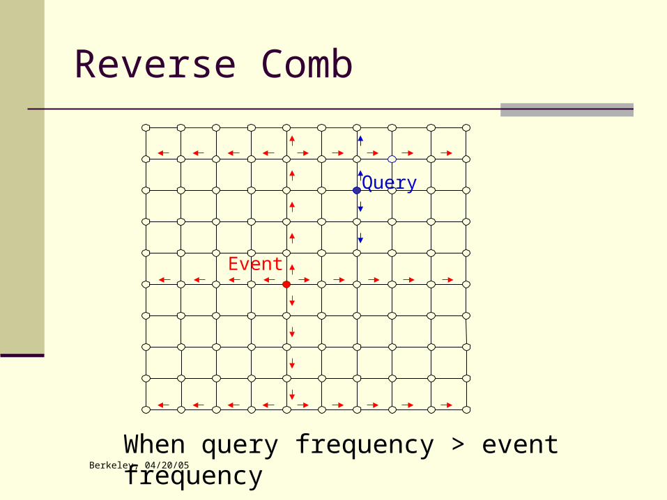
Reverse Comb
Query
Event
When query frequency > event frequency

Berkeley, 04/20/05
The Spectrum of Push and Pull
Pull Push
Global pull +Local push
Global push +Local pull
Push & Pull
Inter-spike spacing increases
Reverse comb
Relative query frequency increases

Berkeley, 04/20/05
Comparison

Berkeley, 04/20/05
Simulations
Radio model Path loss and random error
Topology model Regular grid with random shifts
Routing Constrained Geographical Flooding (CFG) for
random topology Based on simulator Prowler

Berkeley, 04/20/05
An instance of connectivity

Berkeley, 04/20/05
Simulation Cont’d
f_e=1f_q=0.1

Berkeley, 04/20/05
Simulation Cont’d
f_e=1f_q=1

Berkeley, 04/20/05
Random Topology

Berkeley, 04/20/05
Constrained geographical flooding
Needles and combs have certain widths

Berkeley, 04/20/05
Success Rate

Berkeley, 04/20/05
Power consumption

Berkeley, 04/20/05
A few issues
Adaptive scheme Reliability Single fixed query entry point Yes-or-No query

Berkeley, 04/20/05
Adaptive Scheme
Comb granularity depends on the query and event frequencies
Nodes estimate the query and event frequencies Important to match needle length and inter-spike
spacing Comb rotates
Load balancing Broadcast information of current inter-spike spacing

Berkeley, 04/20/05
An illustration
Regular grid Communication cost: hop counts No node failure Adaptive scheme

Berkeley, 04/20/05
Event & Query Frequencies

Berkeley, 04/20/05
Tracking the Ideal Inter-Spike Spacing

Berkeley, 04/20/05
Simulation Results
Gain depends on the query and event frequencies Even if needle length < inter-spike spacing, there is a
chance of success. Tradeoff between success ratio and cost
99.33% success ratio and 99.64% power consumption compared to the ideal case

Berkeley, 04/20/05
Strategies for Improving Reliability
Local enhancement Interleaved mesh Routing update
Spatial diversity Correlated failures Enhance and balance query success rate at
different geo-locations

Berkeley, 04/20/05
Spatial Diversity
Query
xEvent

Berkeley, 04/20/05
Fixed-Node Query
Only one fixed query entry point Depends on relative frequency Depends on the length of the query
E.g., 5 seconds vs. 30 minutes

Berkeley, 04/20/05
Numerical illustration

Berkeley, 04/20/05
Binary query
Is there a tank in the field? Ans: Yes or No. If not delay sensitive
Sequential query process Optimal comb width is shorter
Intuition: can stop earlier

Berkeley, 04/20/05
Numerical illustration

Berkeley, 04/20/05
Summary
Balance query cost vs. event report cost Adapt to system changes
Pull Push
Global pull +Local push
Global push +Local pull
Push & Pull
Relative query frequency increases

Berkeley, 04/20/05
Future work
Data compression A more realistic model for communication
cost Build a fixed comb structure for random
networks for better success rate What if no/limited location knowledge? Consider delay tradeoff Accommodate sleep-awake pattern

Berkeley, 04/20/05
Joint work with P. Mohapatra, C. Chuah, P. Cheng
On the Deployment of Wireless Sensor Networks

Berkeley, 04/20/05
Many-to-One Communication

Berkeley, 04/20/05
Network Deployment
Many-to-one communication Data from all nodes directed to a sink
node/fusion center Unbalanced traffic load Uneven power consumption
Limitations on network lifetime if uniformly distributed “Important” nodes in the route die quickly
Capacity bottleneck and Power bottleneck Desire for long-lived sensor networks
Linear and planar networks

Berkeley, 04/20/05
Precise placement With access Expensive nodes Higher layer of a hierarchical structure
Random placement No access Cheap nodes Lower layer of the hierarchy Coverage and connectivity properties
Precise vs. Random Placement

Berkeley, 04/20/05
Maximize coverage area Given the desired lifetime and # of node
available Maximize the lifetime of the network
Given the number of nodes and coverage area Minimize the number of nodes required
Given the coverage area and the desired lifetime
Consider large networks with long lifetime requirements
Objectives

Berkeley, 04/20/05
Why linear networks? Applications: Traffic monitoring, border line control,
train rail monitoring, etc. Abstract model for narrow-and-long applications
Duck island Tractability, insights for general cases
Highly asymmetric traffic load & location-dependent power consumption
Focus on communications What options do we have?
Linear Networks

Berkeley, 04/20/05
Possible Solutions
More energy for nodes with heavier load
More nodes in the area closer to the sink
Nodes closer to each other
Load balancingPlacement involves
topology control, routing, power allocation

Berkeley, 04/20/05
System Model

Berkeley, 04/20/05
Total energy constraint: (n-1)E Energy can be arbitrarily allocated among
nodes The network dies when no energy left
Thus,
i
Total Energy Constraint

Berkeley, 04/20/05
Problem Formulation
Numerical results as benchmark

Berkeley, 04/20/05
Homogenous initial energy allocation Observation: longer hops consume
more energy “jump” may not be a good idea
Observation: we do not want residual energy when the network dies. Power consumption per unit time should
be the same for all nodes Consider large T (desired lifetime)
A Greedy Algorithm

Berkeley, 04/20/05
A Greedy Algorithm

Berkeley, 04/20/05
Numerical Result

Berkeley, 04/20/05
Performance Analysis
Lifetime, power, and coverage
=4, 19% more node to double lifetime
=4, 138% more node to double coverage
Berkeley, 04/20/05
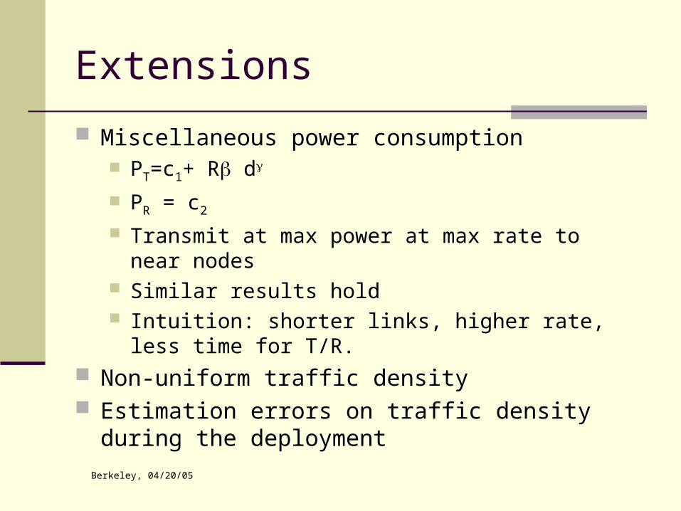
Extensions
Miscellaneous power consumption PT=c1+ R d
PR = c2
Transmit at max power at max rate to near nodes Similar results hold Intuition: shorter links, higher rate, less time for T/R.
Non-uniform traffic density Estimation errors on traffic density during the
deployment

Berkeley, 04/20/05
The effect of arbitrary energy allocation is negligible
Greedy algorithm Compensate for nodes with heavy load by
reducing communication distance Performs very well and adapts to various
conditions 2-D case Data aggregation
Summary

Berkeley, 04/20/05


