
Comparison of different solution strategies for structure deformation using hybrid
OpenMP-MPI methodsMiguel Vargas, Salvador Botello
1/29
Description of the problem
Description of the problem
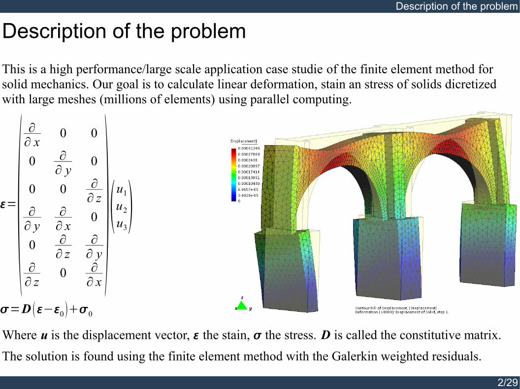
This is a high performance/large scale application case studie of the finite element method for solid mechanics. Our goal is to calculate linear deformation, stain an stress of solids dicretized with large meshes (millions of elements) using parallel computing.
=∂∂ x
0 0
0 ∂∂ y
0
0 0 ∂∂ z
∂∂ y
∂∂ x
0
0 ∂∂ z
∂∂ y
∂∂ z
0 ∂∂ x
u1
u2
u3
=D −0 0
Where u is the displacement vector, the stain, the stress. D is called the constitutive matrix.The solution is found using the finite element method with the Galerkin weighted residuals.
2/29
Description of the problem
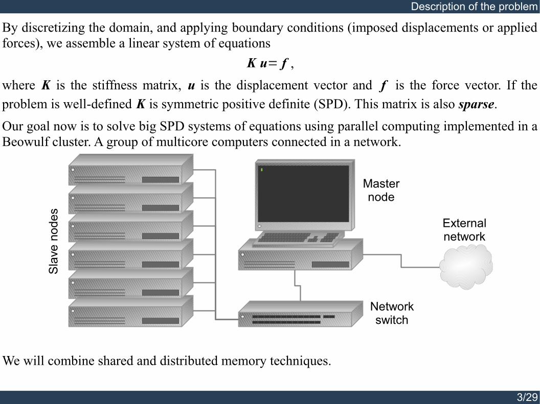
By discretizing the domain, and applying boundary conditions (imposed displacements or applied forces), we assemble a linear system of equations
K u= f ,where K is the stiffness matrix, u is the displacement vector and f is the force vector. If the problem is well-defined K is symmetric positive definite (SPD). This matrix is also sparse.Our goal now is to solve big SPD systems of equations using parallel computing implemented in a Beowulf cluster. A group of multicore computers connected in a network.
Sla
ve n
odes
Masternode
Networkswitch
Externalnetwork
We will combine shared and distributed memory techniques.
3/29
“Divide et impera” with MPI
“Divide et impera” with MPI
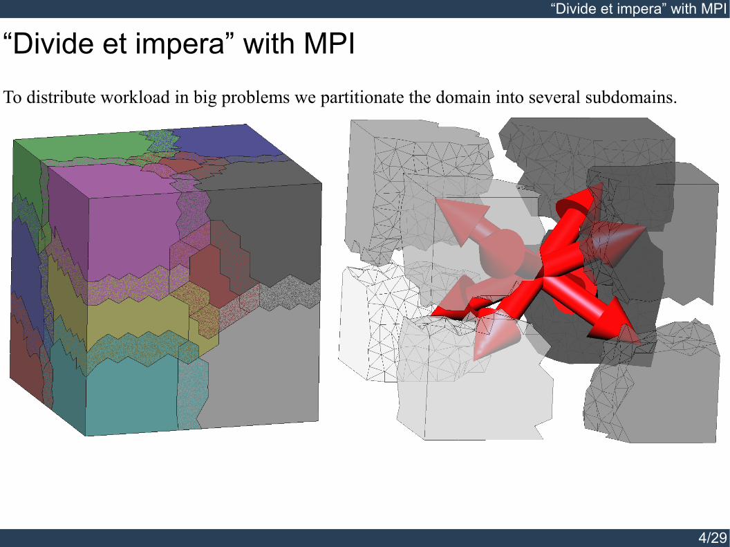
To distribute workload in big problems we partitionate the domain into several subdomains.
4/29

Domain decomposition (Schwarz alternating method)
Domain decomposition (Schwarz alternating method)
This is an iterative method to split a big problem in small problems.
21
∂2
∂
∂1
2 1
∂1 ∖1
∂2∖2
We have a domain with boundary ∂.L is a differential operator L x= y in .Dirichlet conditions x=b on ∂.The domain is divided in two partitions 1
and 2 with boundaries ∂1 and ∂2.
Partitions 1 y 2 are overlapped, =1∪2.1 and 2 are artificial boundaries, they belong to ∂1 and ∂2 and exist inside .
5/29

Domain decomposition (Schwarz alternating method)
2 1
∂1 ∖1
∂2∖2
x10, x2
0 initial approximationswhile ∥x1
i −x1i−1∥ or ∥x 2
i −x2i−1∥
Solve L x1i = y in 1 Solve L x2
i = y in 2
with x1i=b in ∂1∖ 1 with x2
i =b in ∂2∖ 2
Update x1i x2
i−1∣1in 1 Update x2
i x1i−1∣2
in 2
i i1Adding overlapping improves convergence:
1
2
2
1
1
2
1
2
6/29

Domain decomposition (Schwarz alternating method)
Implementation using MPIMPI (Message Passing Interface is a set of routines and programs to make easy to implement and administrate applications that ejecute several processes at the same time. It has routines to transmit data with great efficiency. It could be used in Beowulf clusters.
Network switch
Node
NIC
Processor Processor
Node
NIC
Processor Processor
NodeProcessor
NIC
Processor
Memory
NodeProcessor
NIC
Processor
Memory
NodeProcessor
NIC
Processor
Memory
Memory Memory
• The idea is to assing a MPI process to handle and solve each partition.• OpenMP is used in each MPI process to solve the system of equations of the partition.• Values on artificial boundaries are interchanged using MPI message routines.• Schwarz iterations continue until global convergence is achived.• For partitioning we used METIS library.
7/29

Domain decomposition (Schwarz alternating method)
0 3 6 9 12 15 18 21 24 27 30 33 36 39 42 45 48 51 54 57 60 63 66 69 72 75 78
1E-7
1E-6
1E-5
1E-4
1E-3
1E-2
1E-1
1E+0
1E+1
P1 P2 P3 P4
Iteration
norm
(x' -
x)/n
orm
(x)
d i=∥ut−1
i −uti∥
∥uti∥
8/29

Solving SPD sparse systems ofequations using shared memory
Solving SPD sparse systems ofequations using shared memory
A simple but powerful way to program a multicore computer with shared memory is OpenMP.
MotherboardProcessorCore
32KB L1
Core
32KB L1
ProcessorCore
32KB L1
Core
32KB L1
Bus
RAM
4MB
cach
e L2
4MB
cach
e L2
In modern computers the processor is a lot faster than the memory, between them a high speed memory is used to improve data access. The cache.The most importat issue to achieve high performance is to use the cache efficiently.
Access to CyclesRegister ≤ 1
L1 ~ 3L2 ~ 14
Main memory ~ 240
• Work with use continuous memory blocks.• Access memory in sequence.• Each core should work in an independent memory
area.Algorithms to solve our system of equations should take care of this.
9/29

Solving SPD sparse systems ofequations using shared memory
Parallel preconditioned conjugate gradient for sparse matrices
Preconditioning M A x−b=0 is used to improve CG convergence.Preconditioners must be sparse.
We tested three different preconditioners:
• Jacobi M−1=diag A −1.
• Incomplete Cholesky factorization M−1=G lG l
T, G l≈L.
• Factorized sparse approximate inverese M=H l
TH l, H l≈L−1.
Matrix-vector and dot products are parallelized using OpenMP.Compress row storage method is used to store matrices.Only non-zero entries and their indexes are stored.Entries in each row are contiguos and sorted to improve cache access.Each processor core works with a group of rows to parallelize the operations.
10/29
r0 b−A x0, initial residualp0 M r0, initial descent directionk 0while ∥rk∥
k −r k
TM r k
pkT A pk
xk1 xkk pk
r k1 rk−k A pk
k r k1
T M r k1
r kT M r k
pk1 M r k1k pk
k k1

Solving SPD sparse systems ofequations using shared memory
It looks like:
Vector<T> g(n); // GradientVector<T> p(n); // Descent direcctionVector<T> w(n); // w = A*p
double gg = 0.0;#pragma omp parallel for default(shared) reduction(+:gg) schedule(guided)for (int i = 1; i <= n; ++i){
int* __restrict A_index_i = A.index[i];double* __restrict A_entry_i = A.entry[i];
double sum = 0.0;int k_max = A.count[i];for (register int k = 1; k <= k_max; ++k){
sum += A_entry_i[k]*x.entry[A_index_i[k]];}g.entry[i] = sum - b.entry[i]; // g = AX - b;p.entry[i] = -g.entry[i]; // p = -ggg += g.entry[i]*g.entry[i]; // gg = g'*g
}
int step = 0;while (step < max_steps){
if (Norm(gg) <= tolerance) // Test termination condition{
break;}
double pw = 0.0;#pragma omp parallel for default(shared) reduction(+:pw) schedule(guided)for (int i = 1; i <= n; ++i){
int* __restrict A_index_i = A.index[i];
double* __restrict A_entry_i = A.entry[i];
double sum = 0.0;int k_max = A.count[i];for (register int k = 1; k <= k_max; ++k){
sum += A_entry_i[k]*p.entry[A_index_i[k]];}w.entry[i] = sum; // w = APpw += p.entry[i]*w.entry[i]; // pw = p'*w
}
double alpha = gg/pw; // alpha = (g'*g)/(p'*w)
double gngn = 0.0;#pragma omp parallel for default(shared) reduction(+:gngn)for (int i = 1; i <= n; ++i){
x.entry[i] += alpha*p.entry[i]; // Xn = x + alpha*pg.entry[i] += alpha*w.entry[i]; // Gn = g + alpha*wgngn += g.entry[i]*g.entry[i]; // gngn = Gn'*Gn
}
double beta = gngn/gg; // beta = (Gn'*Gn)/(g'*g)
#pragma omp parallel for default(shared)for (int i = 1; i <= n; ++i){
p.entry[i] = beta*p.entry[i] - g.entry[i]; // Pn = -g + beta*p}
gg = gngn;++step;
}
11/29

Solving SPD sparse systems ofequations using shared memory
Parallel Cholesky factorización for sparse matrices
K=L LT, it is expensive to store and calculate L entries
Li j=1
L j jK i j−∑
k=1
j−1
Li k L j k, for i j
L j j=K j j−∑k=1
j−1
L j k2 .
Stiffnes matrix Cholesky factorization
nnz K =1810 nnz L =8729
nnz K ' =1810 nnz L ' =3215
12/29

Solving SPD sparse systems ofequations using shared memory
We used several strategies to make Cholesky factorization efficient:• Matrix ordering to reduce factorization fill-in. Minimum degree algorithm or nested disection
algorithm (METIS library).• Symbolic Cholesky factorization to determine non-zero entries before calculation.• Factorization matrix is stored using compress row storage to improve forward-substitution.• LT is stored to improve speed of back-substitution.• The fill of each column of L is calculated in parallel using OpenMP.
Core 1
Core 2
Core N
This algorithm is also used to generate the incomplete Cholesky preconditioner.13/29

Solving SPD sparse systems ofequations using shared memory
It looks like:
for (int j = 1; j <= L.columns; ++j){
double* __restrict L_entry_j = L.entry[j];double* __restrict Lt_entry_j = Lt.entry[j];
double L_jj = A(j, j);int L_count_j = L.count[j];for (register int q = 1; q < L_count_j; ++q){
L_jj -= L_entry_j[q]*L_entry_j[q];}L_jj = sqrt(L_jj);L_entry_j[L_count_j] = L_jj; // L(j)(j) = sqrt(A(j)(j)-sum(k=1, j-1, L(j)(k)*L(j)(k)))Lt_entry_j[1] = L_jj;
int Lt_count_j = Lt.count[j];#pragma omp parallel for default(shared) schedule(guided)for (int q = 2; q <= Lt_count_j; ++q){
int i = Lt.index[j][q];
double* __restrict L_entry_i = L.entry[i];
double L_ij = A(i, j);
const register int* __restrict L_index_j = L.index[j];const register int* __restrict L_index_i = L.index[i];
register int qi = 1;register int qj = 1;register int ki = L_index_i[qi];register int kj = L_index_j[qj];
for (bool next = true; next; ){
while (ki < kj){
++qi;ki = L_index_i[qi];
}while (ki > kj){
++qj;kj = L_index_j[qj];
}while (ki == kj){
if (ki == j){
next = false;break;
}L_ij -= L_entry_i[qi]*L_entry_j[qj];++qi;++qj;ki = L_index_i[qi];kj = L_index_j[qj];
}}L_ij /= L_jj;L_entry_i[qi] = L_ij; // L(i)(j) = (A(i)(j)-sum(k = 1, j-1, L(i)(k)*L(j)(k)))/L(j)(j)Lt_entry_j[q] = L_ij;
}}
14/29
Solving SPD sparse systems ofequations using shared memory
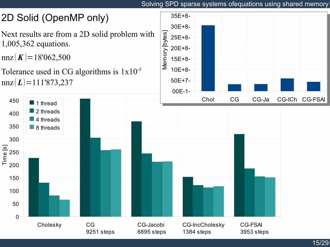
2D Solid (OpenMP only)Next results are from a 2D solid problem with 1,005,362 equations.
nnz K =18'062,500
Tolerance used in CG algorithms is 1x10⁻⁵
nnz L =111'873,237
15/29
Cholesky CG9251 steps
CG-Jacobi6895 steps
CG-IncCholesky1384 steps
CG-FSAI3953 steps
0
50
100
150
200
250
300
350
400
450 1 thread2 threads4 threads8 threads
Tim
e [s
]
Chol CG CG-Ja CG-ICh CG-FSAI00E-1-
50E+7-
10E+8-
15E+8-
20E+8-
25E+8-
30E+8-
35E+8-
Mem
ory
[byt
es]

Solving SPD sparse systems ofequations using shared memory
3D solid (OpenMP only)Elements: 264,250Nodes: 326,228Variables: 978,684nnz(A): 69,255,522nnz(L): 787,567,656
Cholesky CG CG-Jacobi CG-FSAI0
50
100
150
200
250
300
350
400
1 core 2 cores 4 cores 6 cores 8 cores
Tim
e [m
]
Solver 1 core [m] 2 cores [m] 4 cores [m] 6 cores [m] 8 cores [m] MemoryCholesky 142 73 43 34 31 19,864’132,056CG 387 244 152 146 141 922’437,575CG-Jacobi 159 93 57 53 54 923’360,936CG-FSAI 73 45 27 24 23 1,440’239,572
16/29

Now with MPI+OpenMP
Now with MPI+OpenMP
Simulation of a builiding that deformates by self-weight. Basement has fixed displacement. The domain was discretized in 264,250 elements, 326,228 nodes, 978,684 equations,nnz(K) = 69’255,522.
We will solve it using a combination of distributed and shared memory schemas (MPI+OpenMP).17/29

Now with MPI+OpenMP
Results, domain decomposition (14 partitions, 4 threads per solver)Running in 14 computers each one with 4 cores.
Solver Totaltime [s]
Totalmemory
Memoryper slave
Cholesky 347 12,853,865,804 917,054,441CG-FSAI 848 1,779,394,516 126,020,778
CG-Jacobi 2,444 1,149,968,796 81,061,798
Cholesky CG-FSAI CG-Jacobi0
500
1,000
1,500
2,000
2,500
3,000
347
848
2,444
Tim
e [s
]
Cholesky CG-FSAI CG-Jacobi0
2,000,000,000
4,000,000,000
6,000,000,000
8,000,000,000
10,000,000,000
12,000,000,000
14,000,000,000
Mem
ory
[byte
s]
18/29

Now with MPI+OpenMP
Results, domain decomposition (28 partitions, 2 threads per solver)Running in 14 computers each one with 4 cores.
Solver Totaltime [s]
Totalmemory
Memoryper slave
Cholesky 178 12,520,198,517 893,173,100CG-FSAI 686 1,985,459,829 140,691,765
CG-Jacobi 1,940 1,290,499,837 91,051,766
Cholesky CG-FSAI CG-Jacobi0
500
1,000
1,500
2,000
2,500
3,000
178
686
1,941
Tim
e [s
]
Cholesky CG-FSAI CG-Jacobi0
2,000,000,000
4,000,000,000
6,000,000,000
8,000,000,000
10,000,000,000
12,000,000,000
14,000,000,000
Mem
ory
[byt
es]
19/29
Now with MPI+OpenMP
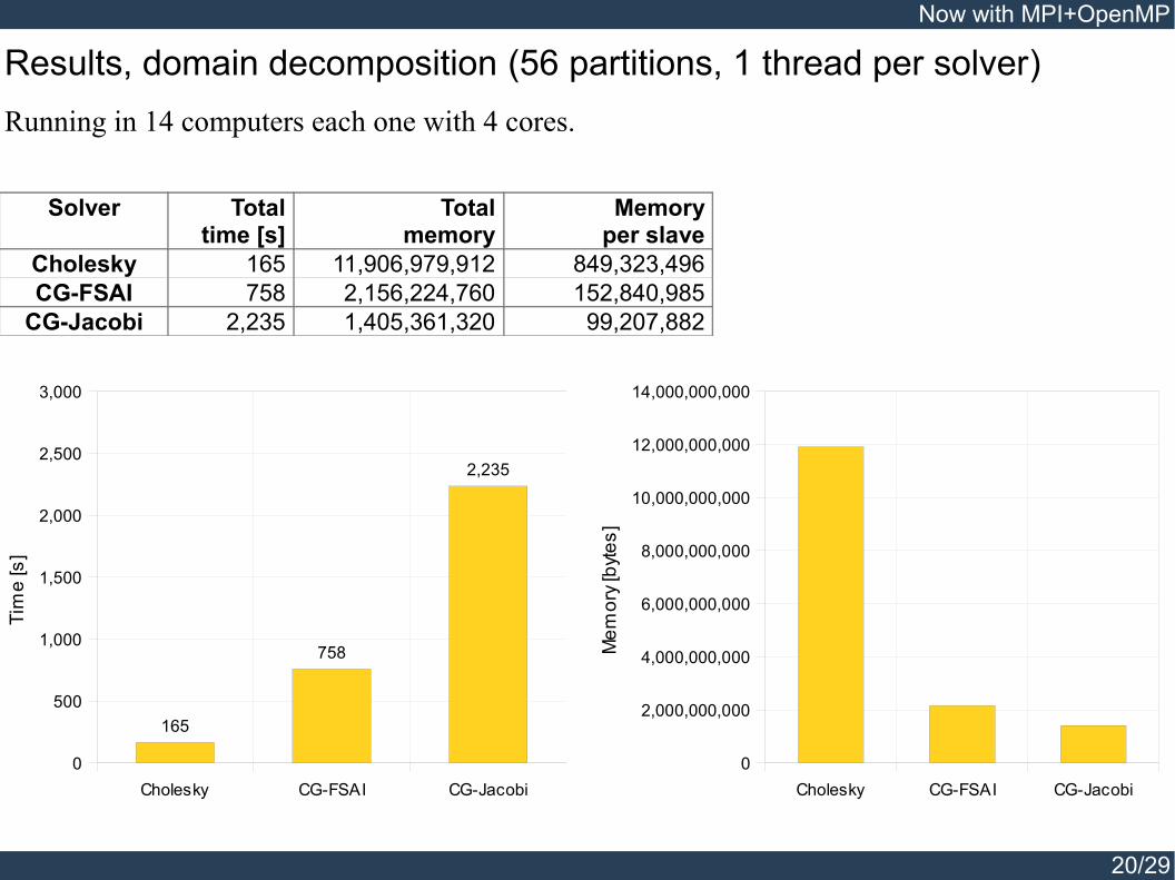
Results, domain decomposition (56 partitions, 1 thread per solver)Running in 14 computers each one with 4 cores.
Solver Totaltime [s]
Totalmemory
Memoryper slave
Cholesky 165 11,906,979,912 849,323,496CG-FSAI 758 2,156,224,760 152,840,985
CG-Jacobi 2,235 1,405,361,320 99,207,882
Cholesky CG-FSAI CG-Jacobi0
500
1,000
1,500
2,000
2,500
3,000
165
758
2,235
Tim
e [s
]
Cholesky CG-FSAI CG-Jacobi0
2,000,000,000
4,000,000,000
6,000,000,000
8,000,000,000
10,000,000,000
12,000,000,000
14,000,000,000
Mem
ory
[byt
es]
20/29

Now with MPI+OpenMP
Comparison264,250 elements,326,228 nodes,978,684 equations,nnz(K) = 69’255,522.
21/29Cholesky CG-Jacobi CG-FSAI
0
500
1000
1500
2000
2500
3000
347
2,444
848
178
1,941
686
165
2,235
758
14 partitions28 partitions56 partitions
Tim
e [s
]
Cholesky CG-Jacobi CG-FSAI0
2,000,000,000
4,000,000,000
6,000,000,000
8,000,000,000
10,000,000,000
12,000,000,000
14,000,000,000
14 partitions28 partitions56 partitions
Mem
ory
[byt
es]

Now with MPI+OpenMP
A bigger exampleElements:Nodes:Equations:nnz(K):Partitions:CPU cores:Nodes:
3’652,9924’011,469
12’034,407794’270,862
124128
31
Solver Time [m] Memory [GB]Cholesky 130 260CG 133,926 34CG-Jacobi 42,510 34CG-FSAI 11,239 42
22/29

Now with MPI+OpenMP
Big systems of equations (2D solid)Equations Time [h] Memory [GB] Cores Overlap Nodes3,970,662 0.12 17 52 12 13
14,400,246 0.93 47 52 10 1332,399,048 1.60 110 60 17 1541,256,528 2.38 142 60 15 1563,487,290 4.93 215 84 17 2978,370,466 5.59 271 100 20 2982,033,206 5.13 285 100 20 29
3,970,662 14,400,246 32,399,048 41,256,528 63,487,290 78,370,466 82,033,2060
1
2
3
4
5
6
0.1
0.9
1.6
2.4
4.9
5.6
5.1
Número de ecuaciones
Tiem
po [h
oras
]
23/29

Lessons learned
Lessons learned
We found that incomple Cholesky factorization is unstable for some matrices, it is posible to stabilize the solver making the preconditioner diagonal-domainant, but we have to use a heuristic.The big issue with iterative solvers is load balancing:
It is complex to partition the domain in such way that local problems take the same time to be solved. This issue is less notizable when Cholesky solver is used.To split the problem using domain decomposition with Cholesky works well, the fastest configuration was using one thread per solver. The good news is that memory is getting cheaper.If memory is a concern we can use CG with FSAI.Next step is to work with gross meshes to have improve approximations.
24/29

Heat diffusion problems
Heat diffusion problems
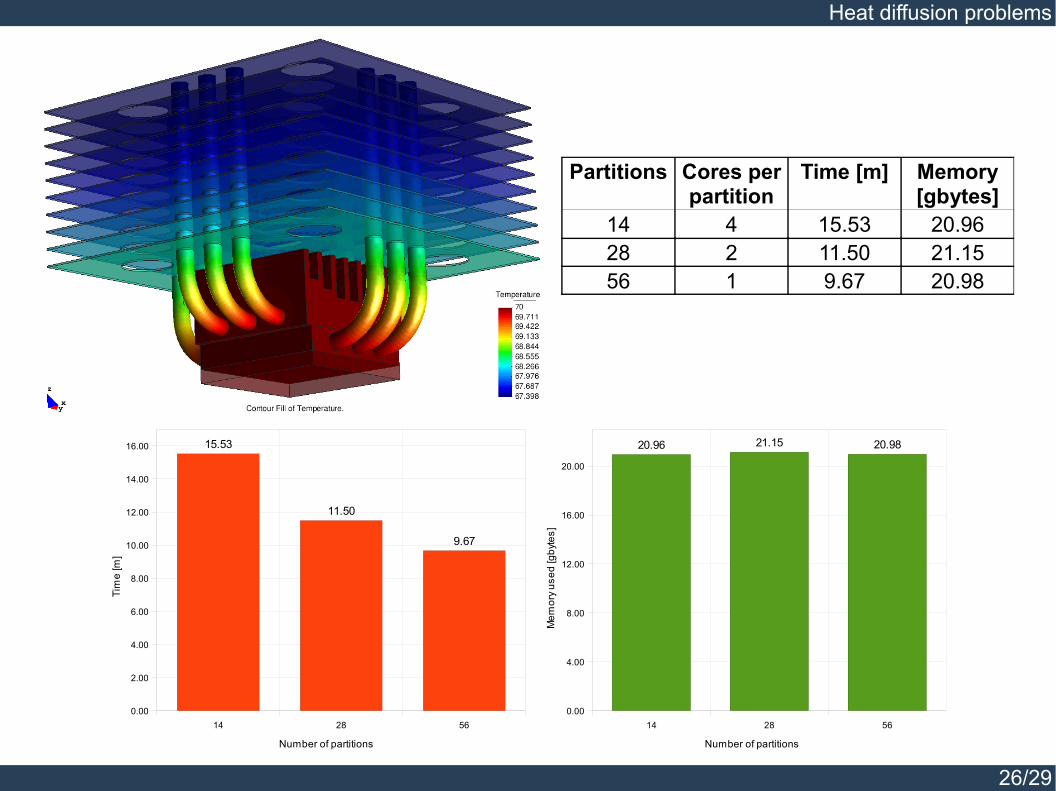
Processor heat sink.
Degrees of freedom 1Dimension 3Element type TetrahedronNodes per element 10Elements 1’409,407Nodes 2’267,539Equations 2’267,539Solver type Cholesky
25/29
Heat diffusion problems
Partitions Cores per partition
Time [m] Memory [gbytes]
14 4 15.53 20.9628 2 11.50 21.1556 1 9.67 20.98
14 28 560.00
2.00
4.00
6.00
8.00
10.00
12.00
14.00
16.00 15.53
11.50
9.67
Number of partitions
Tim
e [m
]
14 28 560.00
4.00
8.00
12.00
16.00
20.00
20.96 21.15 20.98
Number of partitions
Mem
ory u
sed
[gby
tes]
26/29

¿Questions?
¿Questions?
27/29
¿Questions?
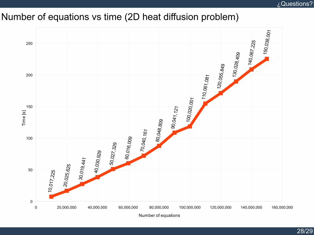
Number of equations vs time (2D heat diffusion problem)
0 20,000,000 40,000,000 60,000,000 80,000,000 100,000,000 120,000,000 140,000,000 160,000,0000
50
100
150
200
25010
,017
,225
20,0
25,6
25
30,0
19,4
41
40,0
30,9
29
50,0
27,3
29
60,0
16,0
09
70,0
40,1
61
80,0
48,8
09
90,0
41,1
21
100,
020,
001 11
0,06
1,08
1
120,
055,
849
130,
028,
409
140,
067,
225
150,
038,
001
Number of equations
Tim
e [s
]
28/29

¿Questions?
Number of equations vs memory (2D heat diffusion problem)
0 20,000,000 40,000,000 60,000,000 80,000,000 100,000,000 120,000,000 140,000,000 160,000,0000
50,000,000,000
100,000,000,000
150,000,000,000
200,000,000,000
250,000,000,000
300,000,000,000
350,000,000,000
10,0
17,2
25
20,0
25,6
25
30,0
19,4
41
40,0
30,9
29
50,0
27,3
29
60,0
16,0
09
70,0
40,1
61
80,0
48,8
09
90,0
41,1
21
100,
020,
001
110,
061,
081
120,
055,
849
130,
028,
409
140,
067,
225
150,
038,
001
Number of equations
Mem
ory
[byt
es]
29/29


