
Computational theory of the responses of V1 & MT neurons and psychophysics of motion perception
~50,000 neurons per cubic mm~6,000 synapses per neuron~10 billion neurons & ~60 trillion synapses in cortex
Neural circuits perform computations
Computational theory: how do neurons compute motion?
Hubel & Wiesel (1968)
V1 orientation tuning

No stimulus in receptive field: no response
Non-preferred stimulus: no response
Preferred stimulus: large response
Orientation selectivity model
linearweighting function
rectification
firing ratestimulus
Complementaryreceptive fields
Rectification and squaring
Rectification and spiking threshold
Stimulus: vertical bar
Responses of each of severalorientation tuned neurons.
Peak (distribution mean) codesfor stimulus orientation.
Distributed representation of orientation
Broad tuning can code for small changes
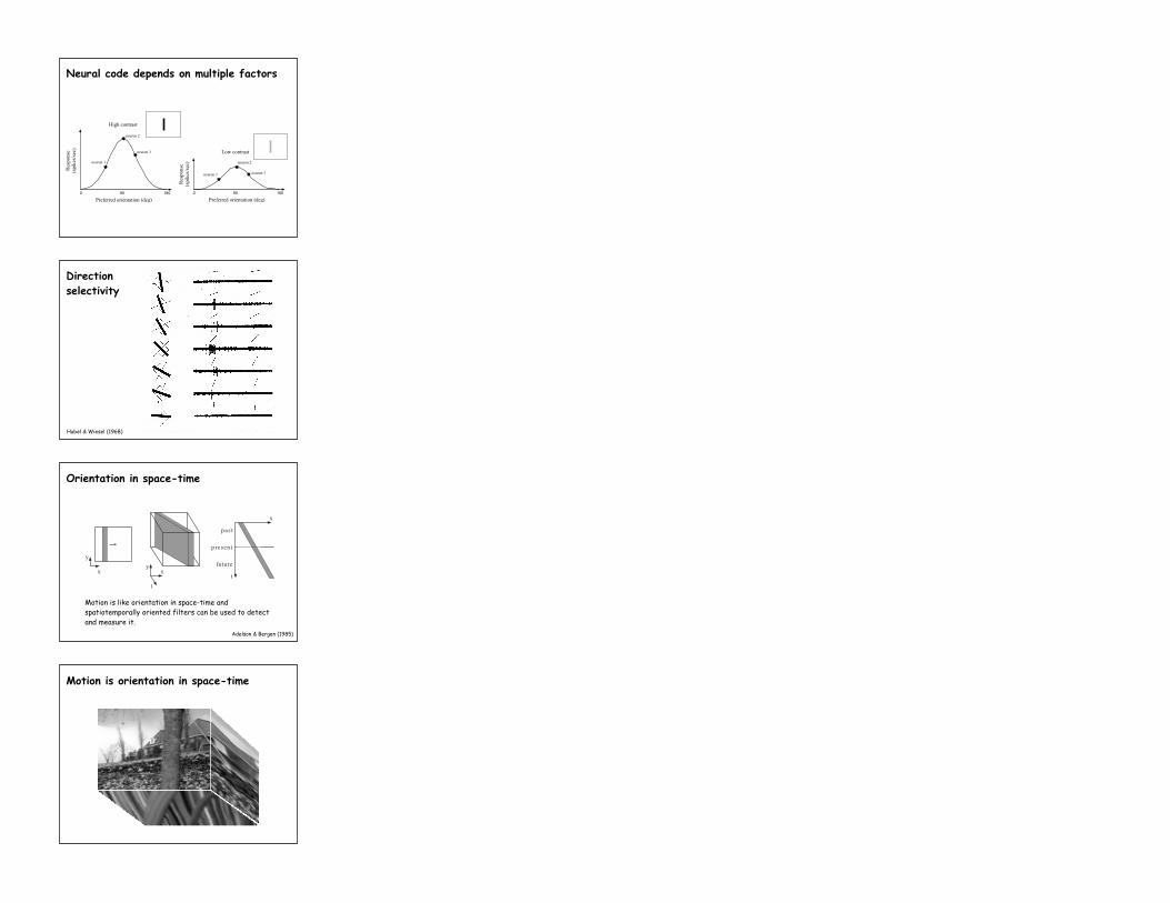
Neural code depends on multiple factors
Direction selectivity
Hubel & Wiesel (1968)
Motion is like orientation in space-time and spatiotemporally oriented filters can be used to detect and measure it.
Orientation in space-time
Adelson & Bergen (1985)
XYTMotion is orientation in space-time

Strong response for motion inpreferred direction.
Weak response for motion innon-preferred direction.
Direction selectivity model
Ohzawa, DeAngelis, & Freeman
Space-time receptive field
t
x
0preferred speed
Population code
Distributed representation of speed
Each spatiotemporal filter computes something like a derivative of image intensity in space and/or time. “Perceived speed” is the orientation corresponding to the gradient in space-time(max response).
Impulse response

Strong response to preferred direction
Note: negative responses not seen in neural firing rates
Weak response to opposite direction
“Aperture Problem”
118 PONTIFICIAE ACADEMIAE SCIENTIARVM SCRIPTA VARTA - 54
Fig. 1. Three different motions that produce the same physical stimulus.
moves to the left. Note that in all three cases the appearance of the
moving grating, as seen through the window, is identical: the bars appear
to move up and to the left, normal to their own orientation, as if produced
by the arrangement shown in Fig. 1A. The fact that a single stimulus can
have many interpretations derives from the structure of the stimulus rather
than from any quirk of the visual system. Any motion parallel to a gra-
ting's bars is invisible, and only motion normal to the bars can be detected.
Thus, there will always be a family of real motions in two dimensions that
can give rise to the same motion of an isolated contour or grating
(Wohlgemuth, 1911, Wallach, 1935; Fennema and Thompson, 1979; Marr
and Ullman, 1981).
[Wallach 1935; Horn & Schunck 1981; Marr & Ullman 1981]
Figure: Movshon, Adelson, Gizzi, Newsome, 1985
The “aperture problem”
These three motions are different but look the same when viewed through a small aperture (i.e., that of a direction-selective receptive field).
Wallach (1935)
Intersection-of-constraints (IOC)
PATTERN RECOGNITION MECHANISMS 123
Fig. 4. A single grating (A) and a 90 deg plaid (B), and the representation of their motions in velocityspace. Both patterns move directly to the right, but have different orientations and 1-D motions. Thedashed lines indicate the families of possible motions for each component.
in spatial extent, and uniformly stimulated the entire retinal region they
covered. This sidesteps the issue which arises in considering stimuli like
the diamond of Fig. 2, of how the identification of spatially separate
moving borders with a common object takes place. Moreover, the plaid
patterns were the literal physical sum of the grating patterns, which makes
superposition models particularly simple to evaluate.
These stimuli were generated by a PDPll computer on the face of
a display oscilloscope, using modifications of methods that are well-
established (Movshon et al., 1978). Gratings were generated by modulat-
[Adelson & Movshon, 1982]
vxvx
vyvy
Intersection of constraints
With two different motion components within the aperture, there is a unique solution:
Adelson & Movshon (1981)

Component vs. pattern motion (perception)
Adelson & Movshon (1981)
+ =weak
pattern-motionpercept
strongpattern-motion
percept+ =
+ =weak
pattern-motionpercept
strongpattern-motion
percept+ =
Adelson & Movshon (1981)
Component vs. pattern motion (perception)
component-motion cell
=
pattern-motion cell
pattern moving up-right strong response
=
grating component moving up-right => strong response
Component vs. pattern motion selectivity
V1 MT
Gratings Plaids
V1
MT
Gratings Plaids
A B C D
E F G H
80
40
80
40
.70
24
12
24
12
.50
Movshon et al., 1983 Model
.25
.35
.50
.25
.70
.35
Simoncelli and Heeger, 1998
Component vs. pattern motion: single neurons

Component gratings
Adapted direction plaids
Mixed direction plaids
Component gratings
Component vs. pattern motion: fMRI adaptation
Huk & Heeger (2002)
74 nature neuroscience • volume 5 no 1 • january 2002
articles
tiples of 90° from trial to trial to minimize adaptation. Theresponse modulations in MT+ were not significantly differentfrom zero (A.C.H., p = 0.35; D.J.H., p = 0.74, two-tailed t-test),demonstrating that the two blocks of plaids elicited similarresponse levels when the effects of both component- and pat-tern-motion adaptation were absent. This result provides furtherevidence that adaptation, due to the repetition of pattern direc-tion, was the key factor in the original experiment.
DISCUSSIONOur findings demonstrate that human MT+ contains a popula-tion of pattern-motion cells and that the activity of those neu-rons is linked to the perception of coherent pattern motion. Thepattern-motion responsivity of human MT+ adds to the case fora homology to macaque MT, which includes a relatively largeproportion of pattern-motion cells1. We also observed lesserdegrees of pattern-motion adaptation in V2, V3, V3A and V4v.Macaque V3 is known to have a minority of pattern-motioncells13, but there are no published investigations of pattern-motion cells in macaque V2, V3A or V4. Although our datademonstrate pattern-motion responses in each of these visualareas, we cannot determine if pattern motion is computed sepa-rately in each visual area or if the responses in V2–V4 are affect-ed by the adaptation that is taking place in MT+. We emphasizethat fMRI adaptation studies14–17 can reveal the selectivities ofsubpopulations of neurons in the human brain, even when thoseneurons are intermingled at a spatial scale that is finer than thespatial sampling resolution (voxel size) of the fMRI measure-ments.
METHODSWe collected fMRI data in 3 subjects, males, 25–39 years old, all withnormal or corrected-to-normal vision. Experiments were undertakenwith the written consent of each subject, and in compliance with the safe-ty guidelines for MR research. Each subject participated in several scan-ning sessions: one to obtain a high-resolution anatomical volume, oneto identify MT+, one to identify the retinotopically organized corticalvisual areas, 2–3 to measure motion adaptation, one to measure base-line responses and 1–3 to perform control measurements. In each subject,we collected 8–20 repeats of the pattern-motion adaptation experimentand 8–16 repeats of the various control experiments.
Stimulus and protocol. Stimuli were presented on a flat-panel display (NEC,multisynch LCD 2000, Itasca, Illinois) placed within a Faraday box with aconducting glass front, positioned near the subjects’ feet. Subjects lay ontheir backs in the MR scanner and viewed the display through binoculars.
Subjects viewed a pair of circular patches 12° in diameter centered 7.5°to the left and right of a central fixation point. Patches were filled witha plaid stimulus comprised of two superimposed sinusoidal gratings.Individual component gratings had 20% contrast, and spatial and tem-poral frequencies were selected to yield a variety of pattern directionswhen superimposed in various combinations (Fig. 1).
Each scan consisted of 6 (32-s) cycles; each cycle consisted of alter-nating adapted-direction and mixed-direction blocks. Adapted-direc-tion blocks consisted of 8 consecutive trials in which the plaid stimulusalways appeared to move in the same direction (horizontally, at 12.9 or1.9°/s; Fig. 1a); mixed-direction blocks consisted of 8 trials in which thedirection of the plaids varied from trial-to-trial (possible plaid direc-tions, computed from the intersection-of-constraints of the componentgratings, were ±31°, ±123° from horizontal at 5.3°/s and 6.3°/s; Fig. 1b).The component gratings with orientations of ±72° had spatial frequen-cies of 0.5 cycles/degree and temporal frequencies of 2 cycles/second (Fig. 1a, components above first plaid); the component gratings withorientations ±45° had spatial frequencies of 0.5 cycles/degree and tem-poral frequencies of 0.67 cycles/second (Fig. 1a, components above sec-ond plaid). In the component-motion experiment, perceptualtransparency was achieved by scaling one component’s spatial frequencyup to 1 cycle/degree and the other down to 0.125 cycle/degree, producinga 3-octave separation. (Temporal frequencies were also scaled accord-ingly to leave component velocities unchanged.)
To control attention, subjects performed a speed discrimination judg-ment on each stimulus presentation16. Each 2-s trial consisted of 1300 ms of plaid motion followed by a 700-ms luminance-matched blankperiod during which subjects pressed a button to indicate which plaid(left or right of fixation) moved faster. The speed differences were deter-mined by an adaptive staircase procedure, adjusting the speeds from trialto trial so that subjects would be approximately 80% correct.
Across different blocks and experiments, we chose to equate percent-correct performance, instead of the exact stimulus speed (although speedsdid remain within a few percent), because in previous work, we and oth-ers have noted large attentional effects on MT+ responses, but no effectsof slight differences in speed18–20. Although the speed discriminationthresholds were larger for non-coherent (transparent gratings) than forcoherent plaids (but not for mixed- versus adapted-direction blocks),the differences were not very large (percent speed-increment thresholdswere !15% versus !10% for non-coherent versus coherent, respective-ly). These small speed differences might affect the responses of someindividual neurons (although speed tuning curves of all direction-selec-tive cells are rather broad), but these speed differences would not beexpected to evoke measurable changes in the pooled activity (as mea-sured with fMRI) of large populations of neurons.
In the adaptation experiments, equal numbers of scans were collectedwith the plaids moving in opposite directions (for example, inward
0 16 32–0.5
0
0.5
fMR
I res
pons
e(p
erce
nt B
OLD
sig
nal)
Pattern motionComponent motion
Adapteddirection
Mixeddirection
Visual area
0
0.1
0.2
V1 V2 V3 V4v V3A MT+
Pat
tern
ada
ptat
ion
inde
x(a
dapt
atio
n re
spon
se/b
asel
ine
resp
onse
)
Pattern motion
Component motion
Time (s)
Fig. 2. Pattern-motion adaptation in human visual cortex. (a) Averagetime series in MT+. Pattern-motion adaptation produced strong modu-lations in MT+ activity. Transparent component motion evoked muchless adaptation. Each trace represents the average MT+ response, aver-aged across subjects and scanning sessions. (b) Adaptation index acrossall visual areas. Pattern-motion adaptation was largest in MT+, but alsoevident in other extrastriate visual areas. Adaptation was weak androughly equal across visual areas in the transparent component-motionexperiment. Height of bars, geometric mean across subjects (arithmeticmean yielded similar results). Error bars, bootstrap estimates of the 68%confidence intervals.
a
b
©20
01 N
atur
e P
ublis
hing
Gro
up h
ttp:
//neu
rosc
i.nat
ure.
com
© 2001 Nature Publishing Group http://neurosci.nature.com
Huk & Heeger (2002)
Visual areaMT+V1 V2 V3 V4v V3A
Mot
ion
adap
tati
on in
dex
(ada
ptat
ion
resp
onse
/ba
selin
e re
spon
se)
Strong pattern motion percept
Weak pattern motion percept
Pattern motion selectivity across visual areas
Pattern motion selectivity model
Simoncelli & Heeger (1998)
Intersection of constraints (two components)
Each component activates a different V1 neuron, selective for a different orientation and speed.

Intersection of constraints (many components)
Each component activates a different V1 neuron, selective for a different orientation and speed.
How do you get selectivity for the moving pattern as a whole, not the individual components?
+ + + +
Answer: For each possible 2D velocity, add up the responses of those V1 neurons whose preferred orientation and speed is consistent with that 2D velocity.
Neural implementation of IOC
t
x
y
Construction of MT pattern cell velocity selectivity via combination
of V1 complex cell afferents, shown in the Fourier domain.
Linear velocity selectivity
Simoncelli, 1993
Add spectral energy on plane
Subtract spectral energy off plane
Spatiotemporal frequency domain
Spatiotemporal frequency response of space-time oriented linear filter.
Frequency responses of filters that are all consistent with one velocity.
!"#$%&&
!'()%*$+"*,$-%./0*"1'2,*,$
!!
!"!#
!
$!
$"
3/45*,%6/2"72"6/8-92,*"6"2,%:8/;:*88%;%,"/;*%,"#"*/,6<
'2,*,$=./0#.*>%:*,"+%*4#$%?@%./0*"1:/4#*,<
A7/72.#"*/,/8"+%6%4%0+#,*6467;/@*:%6#:*6";*52"%:;%7;%6%,?"#"*/,/8@%./0*"1<
AB-CDEFGG
MT
Linear weightingTuning
Simoncelli, 1993
!"#$% &&
!'( )%*$+"*,$ -%./0*"1 '2,*,$
!!
!"!#
!
$!
$"
3/45*,%6 /2"72"6 /8 -9 2,*"6 "2,%: 8/; :*88%;%," /;*%,"#"*/,6<
'2,*,$= ./0#.*>%: *, "+% *4#$%?@%./0*"1 :/4#*,<
A 7/72.#"*/, /8 "+%6% 4%0+#,*646 7;/@*:%6 # :*6";*52"%: ;%7;%6%,?"#"*/, /8 @%./0*"1<
AB-CD EFG G
MT
Linear weighting Tuning
Simoncelli, 1993
Distributed representation of 2D velocity
Brightness at each location represents the firing rate of a single MT neuron with a different preferred velocity. Location of peak corresponds to perceived velocity.
+ + + +
vx
vy

V
Vy
x
V
Vy
x
?
V
Vy
x
Visual motion ambiguity
Visual motion ambiguity
43210-5
0
5
10
15
20
Model
Log Contrast Ratio
43210-5
0
5
10
15
20
5%10% 20%40%
Total Contrast
Subject
Log Contrast Ratio
Per
ceiv
ed D
irec
tion
Bia
s (d
egre
es)
Stone et al. 1990
Total contrast
5%
10%
20%
40%
Stone, Watson, Mulligan 1990
IOC failure
[Stone etal 1990]
Bias in perceived velocity
Stone, Watson, & Mulligan (1990)
Perception is our best guess as to what is in the world, given our current sensory input and our prior experience (Helmholtz, 1866).
Goal: explain “mistakes” in perception as “optimal” solutions given the statistics of the environment.
Bayesian perception
memory
Bayesian models of perception
V
Vy
x
V
Vy
x
?
V
Vy
x
V
Vy
x
V
Vy
x
?
V
Vy
x
Bayesian posteriors
Prior bias for slower speeds
Simoncelli (1993)

Bayesian perception
memory
m
likelihood
v
probability
P(m|v)
Bayesian estimation of velocity
Bayesian perception
posterior
v
pro
bab
ility
P(m|v) P(v) ~ P(v|m)x
prior
Bayesian estimation of velocity
prior
Bayesian perception
v^
v
probability
Bayesian estimation of velocity
Bayesian perception
v^ v^
v
probability
v
prior
Bayesian estimation of velocity
Vx
Vy
stimulus idealization modelVy
Vx
Vx
Vy
Vx
Vy
[Simoncelli & Heeger, ARVO ‘92]
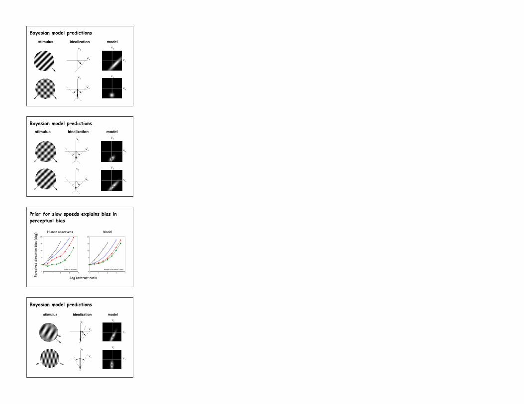
Bayesian model predictions
Vx
Vy
stimulus idealization modelVy
Vx
Vx
Vy
Vx
Vy
Bayesian model predictions
43210
-5
0
5
10
15
20
Model
Log Contrast Ratio
43210-5
0
5
10
15
20
5%10% 20%40%
Total Contrast
Subject
Log Contrast Ratio
Per
ceiv
ed D
irec
tion
Bia
s (d
egre
es)
Stone et al. 1990
[Simoncelli & Heeger, ARVO ‘92]
Log contrast ratio
Human observers Model
Perc
eive
d di
rect
ion
bias
(deg
)
Stone et al (1990) Heeger & Simoncelli (1993)
Prior for slow speeds explains bias in perceptual bias
Vx
Vy
stimulus idealization modelVy
Vx
Vx
Vy
Vx
Vy
Bayesian model predictions

2 1. 5 1 0. 5 0 0.50.5
0.6
0.7
0.8
0.9
1
1.1
Log contrast ratio
Rel
ativ
e sp
eed
max contrast 70%
max contrast 40%
0 1 2 3 4� 5
0
5
10
15
20
25
Log2 contrast ratioB
ias(
degr
ees)
40%
5%
0 20 40 60 80
0
20
40
60
80
100F eature motion
Normal motion
C ontrast
Per
cent
cor
rect
1 2 3 4 5� 80
� 60
� 40
� 20
0
20
40
60
80
C ondition
Dire
ctio
n (d
egre
es)
IOC
0 10 20 30 40 50250
260
270
280
290
300V A
IOC
P laid component separation (degrees)
Judg
ed p
laid
dire
ctio
n
0.4 0.5 0.6 0.7 0.8
0
20
40
60
80
100
R atio of component speeds P
erce
ntag
e in
VA
dire
ctio
n
V A
IOC
Stone & Thompson, ‘90 Stone etal, ‘90 Lorenceau etal, ‘92
Yo & Wilson, ‘92 Burke & Wenderoth, ‘93 Bowns, ‘96
[Weiss, Simoncelli, Adelson, ‘02]
Weiss, Simoncelli, & Adelson (2002)see also Stocker & Simoncelli (2006)
Theory fits lots of behavioral data
The “big picture”
•Functional specialization and computational theory (two balancing principles in the field).
•Canonical computation (linear sum, threshold or sigmoid nonlinearity, adaptation).
•Perception is an inference that has evolved/developed to match the statistics of the environment (Bayesian estimation with priors that embody statistics of environment).
A computational theory of motion appearance
L+M+SL-M L+M-S
A computational theory of color appearance

What distinguishes neural activity that underlies conscious visual appearance?
- Neural activity in certain brain areas.
- Activity of specific subtypes of neurons.
- Particular temporal patterns of neural activity (e.g., oscillations).
- Synchronous activity across groups of neurons in different brain areas.
- Neural activity that is driven by a coherent combination of bottom-up sensory information and top-down recurrent processing (e.g., linked to attention).
- Nothing. Once you know the computations, you’re done!


