HAL Id: hal-00304231https://hal.archives-ouvertes.fr/hal-00304231
Submitted on 5 Jun 2008
HAL is a multi-disciplinary open accessarchive for the deposit and dissemination of sci-entific research documents, whether they are pub-lished or not. The documents may come fromteaching and research institutions in France orabroad, or from public or private research centers.
L’archive ouverte pluridisciplinaire HAL, estdestinée au dépôt et à la diffusion de documentsscientifiques de niveau recherche, publiés ou non,émanant des établissements d’enseignement et derecherche français ou étrangers, des laboratoirespublics ou privés.
Continuous monitoring of the boundary-layer top withlidar
H. Baars, A. Ansmann, R. Engelmann, D. Althausen
To cite this version:H. Baars, A. Ansmann, R. Engelmann, D. Althausen. Continuous monitoring of the boundary-layertop with lidar. Atmospheric Chemistry and Physics Discussions, European Geosciences Union, 2008,8 (3), pp.10749-10790. �hal-00304231�
ACPD
8, 10749–10790, 2008
Boundary-layer top
from lidar
H. Baars et al.
Title Page
Abstract Introduction
Conclusions References
Tables Figures
◭ ◮
◭ ◮
Back Close
Full Screen / Esc
Printer-friendly Version
Interactive Discussion
Atmos. Chem. Phys. Discuss., 8, 10749–10790, 2008
www.atmos-chem-phys-discuss.net/8/10749/2008/
© Author(s) 2008. This work is distributed under
the Creative Commons Attribution 3.0 License.
AtmosphericChemistry
and PhysicsDiscussions
Continuous monitoring of the
boundary-layer top with lidar
H. Baars, A. Ansmann, R. Engelmann, and D. Althausen
Leibniz Institute for Tropospheric Research, Leipzig, Germany
Received: 10 April 2008 – Accepted: 7 May 2008 – Published: 5 June 2008
Correspondence to: H. Baars ([email protected])
Published by Copernicus Publications on behalf of the European Geosciences Union.
10749

ACPD
8, 10749–10790, 2008
Boundary-layer top
from lidar
H. Baars et al.
Title Page
Abstract Introduction
Conclusions References
Tables Figures
◭ ◮
◭ ◮
Back Close
Full Screen / Esc
Printer-friendly Version
Interactive Discussion
Abstract
Continuous lidar observations of the top height of the boundary layer (BL top) have
been performed at Leipzig (51.3◦
N, 12.4◦
E), Germany, since August 2005. The re-
sults of measurements taken with a compact, automated Raman lidar over a one-year
period (February 2006 to January 2007) are presented. Four different methods for the5
determination of the BL top are discussed. The most promising technique, the wavelet
covariance algorithm, is improved by implementing some modifications so that an au-
tomated, robust retrieval of BL depths from lidar data is possible. Three case studies of
simultaneous observations with the Raman lidar, a vertical-wind Doppler lidar, and ac-
companying radiosonde profiling of temperature and humidity are discussed to demon-10
strate the potential and the limits of the four lidar techniques at different aerosol and
meteorological conditions. The lidar-derived BL top heights are compared with respec-
tive values derived from predictions of the regional weather forecast model COSMO of
the German Meteorological Service. The comparison shows a general underestima-
tion of the BL top by about 20% by the model. The statistical analysis of the one-year15
data set reveals that the seasonal mean of the daytime maximum BL top is 1400 m in
spring, 1800 m in summer, 1200 m in autumn, and 800 m in winter at the continental,
central European site. BL top typically increases by 100–300 m per hour in the morning
of convective days.
1 Introduction20
The boundary layer (BL) is directly influenced by the Earth’s surface and responds
to surface forcing by frictional drag, evaporation and transpiration, and sensible heat
transfer with a timescale of an hour or less (Stull, 1988). Vertical fluxes of latent
and sensible heat throughout the BL have thus a strong impact on local and regional
weather. Regarding air quality, the BL height determines the volume available for pollu-25
tant dispersion and the resulting concentrations and is therefore one of the fundamental
10750

ACPD
8, 10749–10790, 2008
Boundary-layer top
from lidar
H. Baars et al.
Title Page
Abstract Introduction
Conclusions References
Tables Figures
◭ ◮
◭ ◮
Back Close
Full Screen / Esc
Printer-friendly Version
Interactive Discussion
parameters in many dispersion models. Continuous observation of the BL top with high
vertical and temporal resolution is thus desirable to support weather and air-quality pre-
diction.
The top of the BL can be determined in several ways (Beyrich, 1997; Cohn and
Angevine, 2000; Seibert et al., 2000; Emeis et al., 2004; Wiegner et al., 2006). Active5
remote sensing of meteorological parameters, trace gases, and aerosols by means of
sodar, radio acoustic sounding system, wind profiler, ceilometer, and lidar appears to
be most appropriate for a continuous BL top detection. All of these instruments, how-
ever, have their restrictions regarding weather conditions, spatial and temporal resolu-
tion, measurement range, and accuracy.10
Lidar permits the detection of the BL top with a vertical resolution of a few meters
and a temporal resolution in the range of seconds to minutes. Lidar has no limitation
regarding measurement range. Even the highest BL tops of 3–4 km in Europe or 4–
6 km over the Sahara can be detected. Aerosol is used as tracer. The only limitation
arises from light attenuating water clouds with optical depth >2. In the presence of a15
cumulus cloud deck, the BL top cannot be detected. But in any case of broken cloud
fields as it is usually the case during convectively active days, lidars will always be able
to detect the BL top.
It has been criticized that unattended, continuous operation of a lidar is not possible
because of security reasons, and that lidar is not able to detect rather low BL tops.20
This is no longer true. By using a small radar the laser beam can be blocked when-
ever an aircraft appears in a well-defined cone above the lidar site. Accurate alignment
of the lidar (laser-beam receiver field-of-view), the potential to measure several sig-
nals simultaneously, and the fact that a lidar can easily be equipped with a near-range
and a far-range telescope, guarantees high-quality BL top detection even at heights25
lower than 100 m if this is a requirement. Furthermore, in recent years several efforts
have been undertaken to develop the software for an automated analysis of lidar data,
e.g., regarding aerosol/cloud discrimination, aerosol layer identification, and for an au-
tomated retrieval of aerosol backscatter and extinction profiles (Campbell et al., 2002;
10751

ACPD
8, 10749–10790, 2008
Boundary-layer top
from lidar
H. Baars et al.
Title Page
Abstract Introduction
Conclusions References
Tables Figures
◭ ◮
◭ ◮
Back Close
Full Screen / Esc
Printer-friendly Version
Interactive Discussion
Turner et al., 2002; Liu et al., 2004; Morille et al., 2007; Althausen et al., 2008).
Several lidar techniques for BL top detection have been suggested (Russel et al.,
1974; Hooper and Eloranta, 1986; Piironen and Eloranta, 1995; Flamant et al., 1997;
Menut et al., 1999; Steyn et al., 1999; Cohn and Angevine, 2000; Brooks, 2003). The
ideas behind the methods are described in Sect. 3. Latest applications, comparisons5
and discussions of these methods can be found in Lammert and Bosenberg (2005),
Martucci et al. (2007), and Morille et al. (2007). We contribute to this discussion by
comparing the available methods for a variety of different aerosol and meteorological
conditions. We improved the wavelet analysis technique (Brooks, 2003) which is to
our opinion the most promising one. We introduce modifications that permit an al-10
most automated (objective) analysis of a longterm data set, in our case of a one-year
data set (February 2006–January 2007). In the case studies presented, Doppler lidar
observation of the height profile of the vertical-wind component and radiosonde mea-
surements of pressure, temperature, and relative humidity were performed in addition.
The Doppler lidar monitors the diurnal cycle of convective activity (upward and down-15
ward motions) with high vertical and temporal resolution and precisely indicates the
beginning of the evolution of the BL in the morning and of the formation of the resid-
ual layer in the late afternoon and thus the collapse of the daytime BL. We compare
the lidar-derived with model-derived BL top heights. The employed weather predic-
tion model COSMO (Consortium for Small-scale Modelling) is a regional scale weather20
forecast model of the German Meteorological Service and provides BL heights on a
hourly basis.
The paper is organized as follows. The compact Raman lidar is described in Sect. 2.
The lidar-based BL top detection methods are briefly explained in Sect. 3. In addition,
the COSMO model approach of BL identification is briefly described. In Sect. 4, the25
modified wavelet covariance technique is outlined. The observations (case studies) are
discussed in Sect. 5. Section 6 presents the main findings of the statistical analysis
of all lidar measurements taken from February 2006 to January 2007. The results
are compared with respective COSMO predictions. A short summary and concluding
10752

ACPD
8, 10749–10790, 2008
Boundary-layer top
from lidar
H. Baars et al.
Title Page
Abstract Introduction
Conclusions References
Tables Figures
◭ ◮
◭ ◮
Back Close
Full Screen / Esc
Printer-friendly Version
Interactive Discussion
remarks are given in Sect. 7.
2 Instrumentation
2.1 Polly
The small and compact Raman lidar Polly (POrtabLe Lidar sYstem, Althausen et al.,
2004) was employed for the study. The setup is shown in Fig. 1a together with a photo5
of the automated lidar (Fig. 1b). A frequency doubled Nd:YAG laser (BigSky model
CFR200) is used as the light source. It emits pulses of 120 mJ at 532 nm wavelength
with a repetition rate of 15 Hz. The light beam is expanded by a factor of 8 which
reduces the divergence of the outgoing beam to less than 0.5 mrad. Two mirrors are
used to transmit the light into the atmosphere and to keep the light beam as close as10
possible to the line-of-sight of the receiver telescope.
The backscattered light is collected with a Newtonian telescope which has a primary
mirror diameter of 20 cm and a focal length of 80 cm. The receiver field of view is
set to 1.25 mrad. After separating and passing the respective interference filters, the
photons elastically backscattered at 532-nm wavelength and the photons inelastically15
(Raman) scattered by nitrogen molecules at 607 nm are detected with photomultipliers
(PMT, Hamamatsu, type R5600P). All signals are amplified and acquired by a photon
counter. The bin width of the data acquisition card (Fast ComTec, model 7882) is
250 ns which results in a spatial resolution of 37.5 m. The maximum (reliable) count
rate of the PMT-preamplifier unit is about 10 MHz.20
The incomplete laser-beam receiver-field-of-view overlap (Wandinger and Ansmann,
2002) restricts the observational range to heights above 200 m in the case of Polly. In
our study we use the elastically backscattered 532 nm lidar return signal. We con-
centrate on the detection of the daytime BL top detection. If a detailed study of the
nighttime BL would be an important issue, we could easily include the retrieval of the25
BL top from the signal ratio of the elastic backscatter signal to the nitrogen Raman
10753
ACPD
8, 10749–10790, 2008
Boundary-layer top
from lidar
H. Baars et al.
Title Page
Abstract Introduction
Conclusions References
Tables Figures
◭ ◮
◭ ◮
Back Close
Full Screen / Esc
Printer-friendly Version
Interactive Discussion
signal. The signal ratio is almost not affected by overlap problems and permits the
detection of all aerosol structures in the lower troposphere down to heights of 50 m.
To avoid large data gaps in the time series caused by potential laser damages we
decided to perform BL observations between minute 8–13 of each hour only. The case
studies in Sect. 5 however are based on continuous lidar observations throughout the5
day (without interruptions) .
It worth noting that Polly can provide much more information of the lower troposphere
than just the BL top height. This small aerosol Raman lidar allows us to measure
height profiles of the volume extinction coefficient profile of the particles at 532 nm,
to estimate the respective particle optical depth, and to determine the extinction-to-10
backscatter ratio (lidar ratio) at nighttime (Ansmann et al., 1992; Ansmann and Muller,
2005). The lidar ratio is useful in the characterization of the aerosol type (Muller et al.,
2007). By using a narrow interference filter (with a spectral width of 0.2 nm instead of
2 nm as used here) in front of the nitrogen Raman channel, aerosol extinction profiling
in the BL is possible even at daytime.15
Polly was moved to China in 2004 to characterize the optical properties of aerosols
over the heavily polluted Pearl River Delta in southern China in the autumn of 2004
(Ansmann et al., 2005; Muller et al., 2006) and over Beijing in January 2005 (Tesche
et al., 2007).
In the last two years we designed a Polly XT (extended version, Althausen et al.,20
2008) which has seven receiver channels for backscatter and extinction profiling at 355
and 532 nm, backscatter profiling at 1064 nm, and to measure the depolarization ratio
at 355 nm. The latter quantity together with the wavelength dependence of the lidar
ratio and the extinction coefficient allows us to unambiguously identify the aerosol type.
The derivation of microphysical properties and of the climate-relevant single scattering25
albedo (scattering-to-extinction ratio) from the Polly-XT data is now possible (Muller
et al., 2005).
10754

ACPD
8, 10749–10790, 2008
Boundary-layer top
from lidar
H. Baars et al.
Title Page
Abstract Introduction
Conclusions References
Tables Figures
◭ ◮
◭ ◮
Back Close
Full Screen / Esc
Printer-friendly Version
Interactive Discussion
2.1.1 WiLi
During days with pronounced BL evolutions discussed below, radiosondes were
launched and the Doppler wind lidar WiLi for vertical-wind observations was operated
in addition. The Doppler lidar emits laser pulses of 1.5 mJ at 2022.5 nm wavelength.
The repetition rate is 750 Hz. Measurements are made with a resolution of 75 m and5
5–30 s. The heterodyne detection scheme allows us to measure line-of-sight wind
speeds in the BL up to 20 m/s with a resolution of about 0.1 m/s. Further details are
given in Zeromskis et al. (2003) and Engelmann et al. (2008). Lowest measurement
height is 400 m.
2.1.2 Radiosonde10
2–3 Vaisala RS-80 radiosondes were launched at the lidar site per day during the ob-
servations presented in Sect. 5 (case studies). The radiosondes provide geopotential
height, temperature T (◦C), and relative humidity RH at the pressure levels. From these
quantities, the water-vapor-to-dry-air mixing ratio and the virtual potential temperature
are calculated.15
3 Methodology
A variety of lidar techniques have been developed to identify the BL top. The best can-
didates are the gradient method (Flamant et al., 1997; Menut et al., 1999), the variance
analysis (Piironen and Eloranta, 1995; Menut et al., 1999), and the wavelet covariance
technique (Cohn and Angevine, 2000; Brooks, 2003). The gradient and the wavelet co-20
variance methods assume that the BL contains much more aerosol particles than the
free troposphere so that a strong decrease of the backscatter signal is observable at
BL top. The variance analysis technique makes use of the strong temporal variation of
the lidar signal at BL top caused by entrainment of clear air from the free troposphere
into the BL.25
10755

ACPD
8, 10749–10790, 2008
Boundary-layer top
from lidar
H. Baars et al.
Title Page
Abstract Introduction
Conclusions References
Tables Figures
◭ ◮
◭ ◮
Back Close
Full Screen / Esc
Printer-friendly Version
Interactive Discussion
The gradient method and the variance analysis approach are illustrated in Fig. 2a
and b, respectively. The substance in Fig. 2a is assumed to be the concentration of
atmospheric aerosol particles, but could also be the water vapor mixing ratio. In the
case of particles, the corresponding lidar signal (after overlap, background and range-
correction) is similar to the profile shown in Fig. 2a.5
In the gradient method, the first (or second) derivation of the corrected lidar signal
with respect to height is used (Flamant et al., 1997; Menut et al., 1999). The minimum
gradient indicates the BL top. Similarly, the variance analysis (Hooper and Eloranta,
1986; Piironen and Eloranta, 1995; Menut et al., 1999) searches for a maximum in the
profile of the sum of the squares of the lidar signal deviations from the mean value of,10
e.g., a five-minute or 1-h measurement period (see Fig. 2c). The maximum is reached
in the center of the transition zone. The transition zone (or entrainment layer) is defined
as the layer in which mixing of polluted boundary-layer and clean free-troposphere air
significantly influence the aerosol concentration at any height within this layer. The
third method is the wavelet covariance transform (WCT) method. This technique is15
described in detail in Sect. 4 and illustrated in Fig. 3.
In the fourth lidar approach (Steyn et al., 1999), the BL top height is determined just
by fitting an idealized backscatter profile to the measured one shown in Fig. 2a. The
idealized profile is characterized by height-independent backscattering in the lower BL,
a smooth decrease of the backscatter signal in the transition zone, and again height-20
independent backscattering in the free troposphere. According to this method the top
of the BL coincides with the center of the transition zone. The idealized function is
defined by four parameters, namely the mean backscatter coefficients in the BL and in
the free troposphere, and the center height (BL top height) and vertical depth of the
transition zone. The fit algorithm searches for the optimum solution (best fit).25
Figure 2d shows how the BL top is obtained from the gradient Richardson number
Ri g. This approach is explained in the next subsection.
10756

ACPD
8, 10749–10790, 2008
Boundary-layer top
from lidar
H. Baars et al.
Title Page
Abstract Introduction
Conclusions References
Tables Figures
◭ ◮
◭ ◮
Back Close
Full Screen / Esc
Printer-friendly Version
Interactive Discussion
3.1 BL top from COSMO model
The non-hydrostatic numerical weather prediction (NWP) model COSMO was devel-
oped at the German Meteorological Service (DWD) as a flexible tool for operational
NWPs on the meso-β (5–50 km) and meso-γ scale (50–500 km) (Fay and Neun-
haeuserer, 2006). The COSMO model used here is operational at the DWD with a5
horizontal resolution of 7 km and 35 vertical layers since the end of 1999. Documenta-
tion is provided at the COSMO web site (http://www.cosmo-model.org).
The operational gradient-Richardson-number scheme is based on the diagnostic ver-
sion of the turbulence parameterisation scheme of COSMO and applied to determined
the height of the BL top. The method searches for the transition from the dynami-10
cally and thermally unstable BL to the stable layer above the BL. A critical Richardson
number (0.38 in the COSMO model) is introduced to identify the top of the BL. The
Richardson number is lower than 0.38 in the turbulent BL and exceeds the critical
value when turbulence production significantly weakens and finally vanishes at the top
of the BL. This is illustrated in Fig. 2d.15
An extended discussion of the critical-Richardson-number approach is given by Zil-
itinkevich and Baklanov (2002). The method is unable to describe a boundary layer in
stable stratification that may extend from heights close to the surface to altitudes above
3 km. Such conditions are often given during nighttime. The method implies that the
boundary layer is in a steady state. Thus, only the equilibrium BL top can be provided20
rather than the actual BL height (Zilitinkevich and Baklanov, 2002).
The critical Richardson number of 0.38 was retrieved from extended comparisons of
COSMO- and radiosonde-derived BL tops in a wide variety of synoptic situations (Fay
et al., 1997). COSMO provides forecasts two times per day for 48 h. BL top heights
are computed for each full hour. The model is initialized at 00:00 and 12:00 UTC.25
To obtain the height at which the gradient Richardson number exactly assumes the
value of 0.38 an interpolation between two model layers is made which leads to an
interpolated height.
10757

ACPD
8, 10749–10790, 2008
Boundary-layer top
from lidar
H. Baars et al.
Title Page
Abstract Introduction
Conclusions References
Tables Figures
◭ ◮
◭ ◮
Back Close
Full Screen / Esc
Printer-friendly Version
Interactive Discussion
Based on validation campaigns it has been found that the BL top height is system-
atically underestimated by approximately 10% to 20%. During convective situations
or periods with frontal passages an underestimation of 30% has been observed (Fay,
1998). Episodes of strong inversions in winter may often not allow the computation of
the BL top height. Nighttime values were found to be usually not reliable. The nighttime5
standard value for Leipzig (rather flat terrain) is set to 389 m.
The minimum BL top height is 200 m in the model. If lower values are computed,
e.g., in cold winter nights, these values are replaced by a BL top height of 200 m. If
no BL top is found below 3000 m or if the atmosphere is non-turbulent at all, a default
value of about 1200 m for Leipzig is computed.10
In this paper, BL tops derived from 00:00- and 12:00-UTC analysis data and the
corresponding 1- to 11-h forecasts are used. We focus on daytime measurements
when the BL top height is usually well defined and located at heights clearly above
500 m.
4 Wavelet covariance transform15
The operation of a fully automated BL lidar includes an automated data analysis. This
in turn implies that a robust method is available that can handle even extreme weather
and aerosol haze situations during all seasons of the year. From extended studies of
the performance of the available lidar methods applied to a large set of lidar observa-
tions we conclude that the wavelet covariance transform (WCT) method is the most20
promising and robust technique for an automated BL top detection. Several thresh-
olds (modifications to the WCT technique) are required to guarantee a successful data
analysis throughout the year. The WCT technique is described in Sect. 4.1. The modi-
fications are presented in Sects. 4.2–4.4.
10758

ACPD
8, 10749–10790, 2008
Boundary-layer top
from lidar
H. Baars et al.
Title Page
Abstract Introduction
Conclusions References
Tables Figures
◭ ◮
◭ ◮
Back Close
Full Screen / Esc
Printer-friendly Version
Interactive Discussion
4.1 Method
The WCT is defined as (Brooks, 2003)
Wf (a, b) =1
a
∫ zt
zb
f (z)h
(
z − b
a
)
dz, (1)
with the Haar function
h
(
z − b
a
)
=
+1, b −a2≤ z ≤ b,
−1, b ≤ z ≤ b +a2,
0, elsewhere.
(2)5
f (z) in Eq. (1) is the range-corrected lidar backscatter signal P (z)z2. z is the measure-
ment height, zb and zt are the lower and upper limits of the lidar return signal profile,
respectively. A Polly lidar signal profile P (z)z2is shown in Fig. 3a. The step function
h(
z−ba
)
is illustrated in Fig. 3b. The dilation a is the extent of the step function. The
translation b determines the location of the step.10
The covariance transform Wf (a, b) is a measure of the similarity of the range-
corrected lidar backscatter signal and the Haar function. In the case of a clear lidar
profile signature as in Fig. 3a with high backscatter values in the BL and significantly
lower backscatter values in the free troposphere, Wf (a, b) takes a clear local maximum
at the height of the BL top provided that an appropriate value of a=n∆z is chosen, as15
is the case for n=12 in Fig. 3c. The height resolution ∆z is 37.5 m in the case of Polly.
The selection of an appropriate value of the dilation a is the main challenge for a
successful retrieval of the BL top height with the WCT method. For rather small values
of a, signal noise dominates the vertical profile of Wf (see Fig. 3c for a=2∆z=75 m).
On the other hand, a too large dilation may not permit us to resolve the BL top when20
further aerosol layers are present in the lower free troposphere. The optimum value for
a is equal to the depth of the transition zone.
10759

ACPD
8, 10749–10790, 2008
Boundary-layer top
from lidar
H. Baars et al.
Title Page
Abstract Introduction
Conclusions References
Tables Figures
◭ ◮
◭ ◮
Back Close
Full Screen / Esc
Printer-friendly Version
Interactive Discussion
Three constraints are introduced in the following to guarantee a robust data analysis.
The first threshold is needed to decide whether the determined BL top height is reliable
or not. Section 4.2 discusses this problem. The problem that signals get increasingly
noisy with height so that aerosol layer identification gets worse and worse with height
is tackled in Sect. 4.3. Finally, data records affected by strongly light-attenuating clouds5
must be identified. Cloud segment identification by means of the WCT is explained in
Sect. 4.4.
4.2 Threshold value of the WCT
A threshold value for the waveform covariance transform WCT is introduced that allows
us to identify a significant gradient and to omit the weak gradients.10
According to Eqs. (1) and (2) and with f (z)=P (z)z2, the discretized form of the WCT
can be written as
Wf (a, b) =1
n∆z
b∑
b− a2
P (z)z2∆z −
b+ a2
∑
b
P (z)z2∆z
=1
n
b∑
b− a2
P (z)z2−
b+ a2
∑
b
P (z)z2
. (3)
The dilation is given by15
a = n∆z, n = 2,4,6,8, ..., (4)
and the position of the translation b has to be chosen in between two discrete data
points to assure an equal number of data points in each integral.
According to Eq. (3), Wf (a, b) can thus be simply expressed by the mean range-
corrected signal values below and above the height of translation b for layers of thick-20
ness a/2. In the next step, we normalize the range-corrected signal by its maximum
10760

ACPD
8, 10749–10790, 2008
Boundary-layer top
from lidar
H. Baars et al.
Title Page
Abstract Introduction
Conclusions References
Tables Figures
◭ ◮
◭ ◮
Back Close
Full Screen / Esc
Printer-friendly Version
Interactive Discussion
value found below 1000 m. This is usually the maximum value of P (z)z2within the BL.
The normalization guarantees the applicability of the threshold method at very different
backscatter conditions in rather clean or very polluted air. An example of a normalized
signal and the corresponding WCT is presented in Fig. 4. Wf (a, b) takes a clear local
maximum with a value of 0.06 for the translation b=bmax=1900 m (height of the BL5
top). A value of 0.06 corresponds to a decrease of the mean signal by about 15–20%
at BL top. A threshold value of 0.05 was found to be sufficient to identify the BL depth.
The first height above ground at which a local maximum of Wf (a, b) occurs, that ex-
ceeds the threshold value of 0.05 is defined as the BL top height zi . If the threshold
condition is not fulfilled, a BL top is not provided by the algorithm.10
As mentioned above, we concentrate on the determination of the height of the day-
time BL top. If nighttime BL observations (e.g., from 17:00–18:00 UTC to 07:00–
08:00 UTC) are of interest, another approach must be developed and another (smaller)
threshold value must be defined to properly identify the BL height close to the ground.
4.3 Height-dependent dilation15
As described above, the choice of a proper dilation a is important. The selection of
a fixed dilation a=12∆z works well except for cases with very shallow BL or very ex-
tended transition zones. Our experience shows that the use of a dilation profile a(z)
described by a quadratic increase of the dilation with height (see Fig. 5) is a good com-
promise to detect very low BL top heights with usually very narrow transition zones, but20
also the extended transition zones (usually observed at heights above 500–1000 m).
4.4 Cloud screening
Clouds are characterized by a steep increase of the range-corrected lidar signal at
the cloud base followed by a strong decrease of the signal with increasing cloud pen-
etration depth. In Fig. 6a such a cloud signal with cloud base at about 1400 m is25
presented. The WCT is shown in Fig. 6b. Due to the definition of the Haar function,
10761

ACPD
8, 10749–10790, 2008
Boundary-layer top
from lidar
H. Baars et al.
Title Page
Abstract Introduction
Conclusions References
Tables Figures
◭ ◮
◭ ◮
Back Close
Full Screen / Esc
Printer-friendly Version
Interactive Discussion
Wf (a, b) has a characteristic shape. It becomes negative at the cloud base and shows
a local minimum before it becomes positive with a local maximum. Thus, the cloud can
be identified by means of a negative threshold. It was found that cloud detection works
very well for a threshold of −0.1 and for a dilation of a=6∆z=225 m. The cloud base
is then one height bin below the altitude at which Wf (a, b) is lower than the chosen5
threshold value. In Fig. 6, cloud base is at 1397 m.
If a cloud is detected in the lidar profile, only values below the cloud base are used
for the determination of the BL top. If no significant gradient can be detected, it is very
probable that this cloud has formed within the BL. In that case, no BL top height is
provided.10
5 Case studies
Three measurement cases obtained at different aerosol and meteorological conditions
are discussed. The evolution of the BL in cloudless conditions is discussed first (11
September 2006). A case with complex aerosol layering (Saharan dust on top of the
BL) observed on 13 September 2008 is presented next. In the third case (4 July 2006),15
cumulus convection complicated the BL top detection. A fourth case is added in which
a systematic deviation between the lidar and COSMO-model-derived BL top height
was observed throughout the entire day although an almost ideal evolution of the BL at
cloudfree conditions occurred.
5.1 11 September 200620
Figure 7 (top) shows the BL evolution in terms of the range-corrected backscatter signal
observed with Polly on 11 September 2006. Sunrise is at about 04:40 UTC, sunset at
17:35 UTC. A steady and almost constant growth of the BL depth is visible with a rate
of 120 m/h from 09:00–14:00 UTC. The maximum depth of the BL of 1175 m is reached
at 15:00 UTC.25
10762

ACPD
8, 10749–10790, 2008
Boundary-layer top
from lidar
H. Baars et al.
Title Page
Abstract Introduction
Conclusions References
Tables Figures
◭ ◮
◭ ◮
Back Close
Full Screen / Esc
Printer-friendly Version
Interactive Discussion
In Fig. 7 (center), WiLi observations of vertical wind speed, and thus of the con-
vective activity, are displayed. The convective period lasts from about 09:00 to almost
16:00 UTC. Vertical motion with upward velocities of up to 2 m/s and downward mo-
tion with up to 1.5 m/s occurs. More details to the 11–13 September period in terms
of aerosol, wind, and aerosol flux measurements are described by Engelmann et al.5
(2008). Simultaneous observations of a backscatter lidar and a wind lidar pointing to
the zenith were first shown by Cohn and Angevine (2000).
Figure 8 presents radiosonde profiles of water-vapor mixing ratio s, temperature T ,
and virtual potential temperature Θv . The first sonde was launched on 11 September
2006, 06:39 UTC and indicates a stable stratification of the atmosphere above 100 m10
height. The second sonde, launched at 13:36 UTC, shows a well-mixed BL with top
height at 1 km.
The results regarding the retrieval of BL top with the available four lidar methods and
from the COSMO model are shown in Fig. 7 (bottom). All lidar methods successfully
determine the height of the BL top between 09:00 and 15:00 UTC. Before 09:00 and15
after 15:00 UTC the presence or the formation of the residual layer causes difficulties,
especially in the case of the 5-min variance method. The signal averaging period of
5 min is too short so that the corresponding signal-to-noise ratio is too large for a proper
determination of the BL top. The development of the nocturnal BL after 18:00 UTC
(see Fig. 7, bottom) as predicted by the COSMO model is not detected with Polly. The20
WCT technique with modifications is unable to resolve layer boundaries close to the
minimum measurement height, i.e., in Fig. 7 below heights of 500 m. Only the gradient
method is able to detect the early-morning BL top before 08:00 UTC by using the first
two signal bins above the minimum measurement height.
The COSMO model underestimates the BL top during the first period of the BL evo-25
lution (09:00–11:00 UTC), provides accurate results around noon and in the early af-
ternoon for the fully developed BL, and also resolves the end of the convective period
shortly before 16:00 UTC as indicated by the WiLi results in Fig. 7b.
As mentioned in Sect. 3.1, the COSMO model is initialized at 00:00 and 12:00 UTC.
10763

ACPD
8, 10749–10790, 2008
Boundary-layer top
from lidar
H. Baars et al.
Title Page
Abstract Introduction
Conclusions References
Tables Figures
◭ ◮
◭ ◮
Back Close
Full Screen / Esc
Printer-friendly Version
Interactive Discussion
BL top forecasts are shown for the periods from 01:00–11:00 UTC and 13:00–
23:00 UTC. Thus the model-derived BL top values presented for the morning hours
(08:00–11:00 UTC) are comparably uncertain, and most accurate for the early-
afternoon period (12:00–14:00 UTC). Routine radiosonde observations by the German
Meteorological Service are performed at three sites around Leipzig. All of them are5
about 150–200 km apart from the lidar site. So even at 12:00 UTC the radiosonde-
based COSMO BL top may not be representative for Leipzig.
The underestimation of the BL top by the COSMO model in the morning (09:00–
11:00 UTC) may also reflect that the critical-gradient-Richardson-number approach
assumes steady state conditions (Zilitinkevich and Baklanov, 2002) as was mentioned10
in Sect. 3.1. This assumption is probably not fully valid during the period of strongest
BL height increase.
5.2 13 September 2006
On 13 September 2006 a Saharan dust layer above the BL complicates the retrieval
of the BL top. The lofted layer is best viewed in the WiLi plot (see Fig. 9, center).15
According to the vertical-wind data the convectively active period lasts from about 10:00
to about 15:30 UTC. Updraft velocities up to 2–3 m/s and downdraft velocities of 1–
2 m/s are measured. The hourly growth rate of the BL depth is roughly 500 m/h from
10:00–11:00 UTC.
Except the fitting method and the 5-min variance analysis (not shown), all lidar re-20
trieval techniques work well at these conditions of complex aerosol layering for the time
period from 08:00–16:00 UTC. Because the signal-to-noise ratio is low, the solutions
of the 5-min variance method show large fluctuations in the BL time series. The fitting
method has problems because a required clear signal step function at BL top is not
given. Note, that the gradient method resolves the BL top at 07:00 and 08:00 UTC, but25
fails after 17:00 UTC. Similarly, the 1-h variance analysis produces uncertain results
in the evening (17:00–19:00 UTC). The WCT technique works best at these complex
conditions of aerosol layering and provides a robust time series from 08:00–19:00 UTC
10764

ACPD
8, 10749–10790, 2008
Boundary-layer top
from lidar
H. Baars et al.
Title Page
Abstract Introduction
Conclusions References
Tables Figures
◭ ◮
◭ ◮
Back Close
Full Screen / Esc
Printer-friendly Version
Interactive Discussion
on this day.
Figure 9 is representative for the majority of analyzed cases of the 2006/2007 data
set. The WCT technique together with the introduced modifications was found to be
the most reliable method for routine BL top detection. In the following, we restrict the
discussion to the comparison of the WCT with COSMO results.5
In Fig. 9, the COSMO model provides the most accurate solution at the initialization
time of 12:00 UTC and in the early morning (07:00–09:00 UTC). The evolution of the
BL top is clearly underestimated by the model at 11:00 UTC (11-h forecast value) and
overestimated at 15:00 UTC, possibly caused by the fact that the radiative impact of
the Saharan dust layer is ignored in the simulations. The growth rate of the BL depth10
is 100 m/h after the COSMO model for the period from 10:00–11:00 UTC instead of
500 m/h as seen by the lidar. The model accurately predicts the end of the BL evolution
close to 16:00 UTC.
5.3 4 July 2006
A high-pressure system over eastern Europe and a low-pressure system over western15
Europe caused the advection of warm and humid air from southern Europe. In contrast
to the cases discussed before, cumulus clouds formed at the top of the BL (see Fig. 10,
top) in the morning of 4 July 2006. The BL reaches heights of about 2 km in the late
afternoon. The BL top height increased by roughly 400 m/h from 08:00–11:00 UTC.
The COSMO model predicts an hourly growth rate of about 250 m/h for this time period.20
The vertical-wind observations in Fig. 10 (center) indicate pronounced updrafts and
downdrafts (up to 3 m/s downward motion) during the daytime from 07:30 to almost
17:00 UTC (18:00 LT). Sunrise and sunset are 03:00 and 19:30 UTC in the beginning
of July.
The BL-height time series obtained with the lidar WCT technique is compared to25
COSMO results in Fig. 10 (bottom). The Polly backscatter color plot indicates that
the lidar detects the BL top even during the phase of cumulus convection. However,
for clarity in the presentation, we omit WCT solutions applied to cloud-screened lidar
10765

ACPD
8, 10749–10790, 2008
Boundary-layer top
from lidar
H. Baars et al.
Title Page
Abstract Introduction
Conclusions References
Tables Figures
◭ ◮
◭ ◮
Back Close
Full Screen / Esc
Printer-friendly Version
Interactive Discussion
signals during the period when clouds developed. Cloud base is indicated by crosses
in Fig. 10 (bottom). The vertical extension from base to top of the clouds varies from
200–400 m. The BL top is thus roughly 100–200 m higher than cloud base (crosses).
Due to technical problems (periodic laser power variations after 12:00 UTC caused
by air conditioning problems) several BL top values could not be determined with suf-5
ficient reliability from the considerably corrupted 5-min signal average profiles around
13:00 UTC and from 14:45–16:00 UTC. The respective BL top values are left out in
Fig. 10.
The COSMO model (6–11-h forecast data) obviously underestimates again the
strength of the BL evolution. After re-initialization at 12:00 UTC, good agreement is10
found between lidar and model solutions. The model also predicts sufficiently well
the time when the convective activity significantly weakens close to 17:00 UTC, as
observed with the Doppler lidar WiLi.
5.4 3 July 2006
The most significant feature in Fig. 11 is the systematic underestimation of the BL top15
height by the COSMO model throughout the day. On average, the difference between
the lidar and the COSMO BL height values is 270 m. In contrast to the 4 July, dry air
was advected to eastern Germany on 3 July 2006 and the influence of a high pressure
system over eastern Europe dominated. The mean growth rate of the BL top height was
150 m/h between 08:00 and 12:00 UTC. The Doppler lidar measured partly vigorous20
upward and downward motions with extreme values close to 3 m/s between 10:30 and
17:00 UTC.
The systematic underestimation of the BL evolution by the COSMO model is most
probably caused by an overestimation of the high pressure influence (large scale sub-
sidence of air) for the Leipzig grid point. The three DWD radiosonde profiles of wind,25
humidity and temperature around Leipzig used to initialize the COSMO model obvi-
ously do not represent the meteorological conditions for the Leipzig area on 3 July,
12:00 UTC. A clear reason for the systematic deviation can however not be given be-
10766

ACPD
8, 10749–10790, 2008
Boundary-layer top
from lidar
H. Baars et al.
Title Page
Abstract Introduction
Conclusions References
Tables Figures
◭ ◮
◭ ◮
Back Close
Full Screen / Esc
Printer-friendly Version
Interactive Discussion
cause of the complex parameterization of turbulence and soil characteristics in the
COSMO model. The forecast model predicts a weakening of the convective activity
as early as 15:00–16:00 UTC, whereas the Doppler lidar (center plot in Fig. 11) ob-
served a strong updraft after 16:00 UTC and the end of the convectively active phase
not before 17:00 UTC.5
The case shown in Fig. 11 demonstrates again that the identification of the night-
time BL top before 07:00 UTC and after 17:00 UTC from lidar data remains a difficult
task. The Doppler lidar indicates that the convective phase lasts from about 07:00–
17:00 UTC on this summer day so that obviously the residual layer top instead of the
BL top is identified by Polly.10
6 Statistical analysis (February 2006–January 2007)
Continuous lidar observation as discussed in Sect. 5 were performed on less than
10% of the days in 2006. The regular measurement program was described in Sect. 2.
Signal profiles were measured with Polly between minute 8–13 of each hour. The
following statistical analysis is based on these five-minute observations. Figure 1215
gives an overview of the data coverage for each month. During 7650 out of the total of
8760 five-minute periods (February 2006 to January 2007) lidar measurements were
possible. Data coverage is thus, on average, 87%. In 3831 cases out of these 7650
five-minute observation periods the BL top height could successfully be determined
with the automated WCT method. Low clouds, the lack of a significant gradient in the20
backscatter profile, or precipitation prohibited the BL depth determination in about 50%
of the measurements.
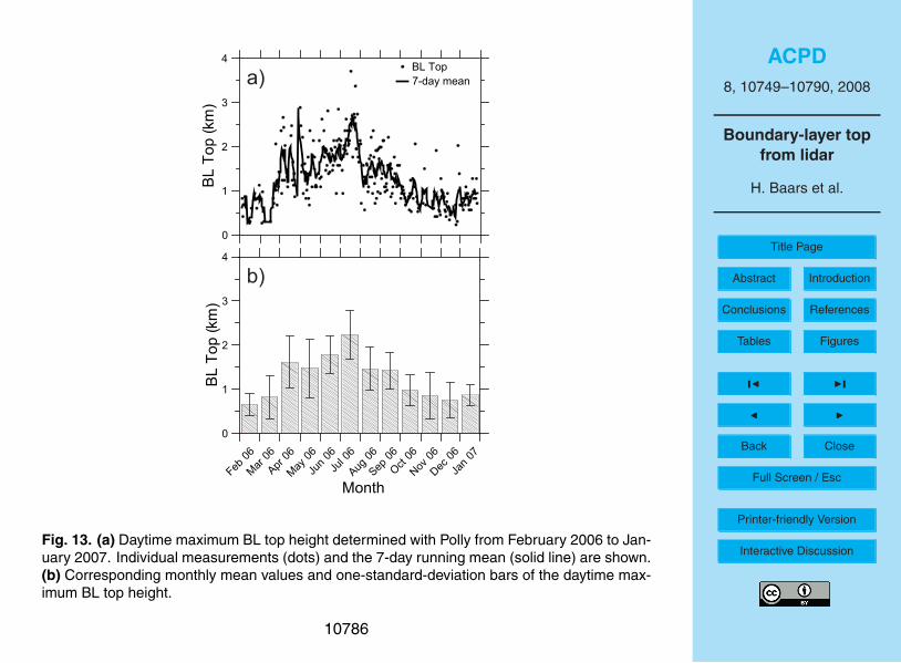
In the following we briefly summarize the main statistical findings. We restrict the
discussion to the daytime data set. In Fig. 13a, the daily maximum BL depths are
plotted together with a running one-week average. A clear seasonal cycle is found.25
Strong convective activity occurs from mid March to the end of September over Leipzig.
Figure 13b shows the corresponding monthly mean values and standard deviations of
10767

ACPD
8, 10749–10790, 2008
Boundary-layer top
from lidar
H. Baars et al.
Title Page
Abstract Introduction
Conclusions References
Tables Figures
◭ ◮
◭ ◮
Back Close
Full Screen / Esc
Printer-friendly Version
Interactive Discussion
the daily maximum values. Whereas, in July 2006 the BL top in the early afternoon
reached values of, on average, 2.2 km (±0.7 km) height, the monthly mean value of
the afternoon BL top height did not exceed 700 m in February 2006. The seasonal
mean of the daytime (08:00–20:00 LT) maximum BL top is 1400 m in spring, 1800 m in
summer, 1200 m in autumn, and 800 m in winter at the continental, central European5
site.
For 65 clear days (without fog, precipitation, and frontal passages combined with
air mass change), the growth of the BL depth in the morning and early afternoon
hours could be studied in detail. On all of these days, the minimum BL height (around
08:00 UTC) could be identified. Figure 14 shows the mean growth rate for the main10
period of the BL evolution. The main period is defined by the time when the BL depth
begins to increase (e.g., 09:00 UTC) and the time when the BL top height reaches
the 0.9 BL daily maximum value (typically 11:00–14:00 UTC). As can be seen, mean
growth rates from about 100–500 m/h were observed. In cases with fast BL growth
of 400–500 m the main phase of the evolution of the BL was two hours or even15
shorter. Large values of 400–500 m/h are observed during the summer season (May
to September).
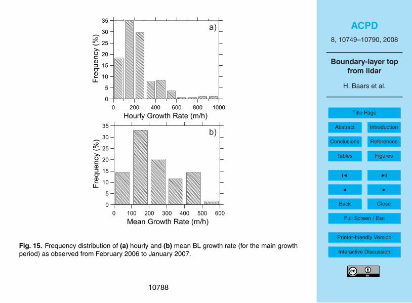
Histograms of observed hourly and mean growth rates are shown in Fig. 15a and b,
respectively. Most hourly growth rates as well as mean growth rates are found between
100 and 300 m/h (about 65%). The largest hourly growth rate of 940 m/h was observed20
on 4 May 2006. The maximum mean growth rate of 510 m/h was observed on 13 July
2006.
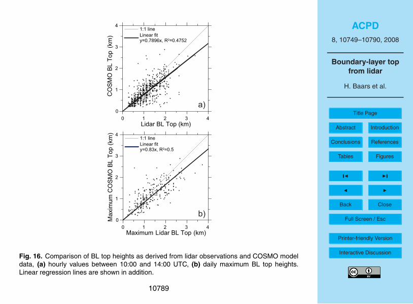
6.1 Comparison with COSMO-derived BL top heights
In Fig. 16 hourly values of the BL top height and of the daily maximum BL top height
determined from lidar data are compared with respective values obtained from the25
COSMO model outputs. Disregarding the large scatter in the data, a systematic un-
derestimation of the daytime BL depth by the COSMO model is visible in both com-
parisons (on average almost 20%). Strong deviations (COSMO BL depth >2000 m,
10768

ACPD
8, 10749–10790, 2008
Boundary-layer top
from lidar
H. Baars et al.
Title Page
Abstract Introduction
Conclusions References
Tables Figures
◭ ◮
◭ ◮
Back Close
Full Screen / Esc
Printer-friendly Version
Interactive Discussion
lidar BL depth <1000 m) occurred in cases with clouds (not predicted by the COSMO
model) or, vice versa, during cloud-free conditions (COSMO BL depth <1000 m, lidar
BL depth >2000 m) when the COSMO model obviously predicted clouds and conse-
quently a suppression of the BL evolution.
The comparison of the daily mean growth rates obtained from Polly and COSMO5
model data for the 65 chosen days is shown in Fig. 17. A reasonable agreement is
observed up to values of about 300 m/h. The corresponding linear regression line for
values below 300 m/h is shown. According to this fit, an underestimation of the mean
BL growth rate by about 25% by the COSMO model is found.
7 Conclusions10
Lidar is a well-established technique for continuous vertical profiling of aerosols
throughout the troposphere. Here, we have shown (and confirmed previous work in
this field) that lidar is also a useful and reliable tool for a continuous and precise mon-
itoring of the daily development of the BL depth. We concluded from comparisons of
the available lidar approaches that the WCT method is of advantage for an automated15
BL top detection. To guarantee a robust data analysis, we introduced some modifica-
tions (thresholds to clearly identify BL top as well as clouds, use of a height-dependent
dilation).
The statistical analysis of the one-year data set revealed that the seasonal mean of
the daytime (08:00–20:00 LT) maximum BL top is 1400 m in spring, 1800 m in summer,20
1200 m in autumn, and 800 m in winter at the continental, central European lidar site.
BL top typically increases by 100–500 m per hour in the morning of convective days.
Mean growth rates were found most frequently between 100 and 300 m/h.
The comparison with COSMO model results showed that the forecast model un-
derestimated the BL top height by, on average, roughly 20% and the evolution of the25
BL (mean growth rate) by about 25%. Strongest deviations occur when clouds are
predicted, but not present and vice versa.
10769

ACPD
8, 10749–10790, 2008
Boundary-layer top
from lidar
H. Baars et al.
Title Page
Abstract Introduction
Conclusions References
Tables Figures
◭ ◮
◭ ◮
Back Close
Full Screen / Esc
Printer-friendly Version
Interactive Discussion
Acknowledgements. We are grateful to the German Meteorological Service for providing the
COSMO model data used in our study. We thank Barbara Fay for providing all the information
about the COSMO model we required and for answering all of our numerous questions.
References
Althausen, D., Engelmann, R., Foster, R., Rhone, P., and Baars, H.: Portable Raman lidar for5
determination of particle backscatter and extinction coefficients, in: Reviewed and revised
papers presented at the 22nd ILRC, ESA SP-561, volume 1, edited by: Pappalardo, G. and
Amodeo, A., 83–86, ESA Publications Division, ESTEC, Noordwijk, The Netherlands, 2004.
10753
Althausen, D., Engelmann, R., Baars, H., Heese, B., and Komppula, M.: Portable Raman lidar10
Polly XT for automatic profile measurements of aerosol backscatter and extinction coefficient,
in: Proceedings, 24th ILRC, edited by: Hardesty, M. and Mayor, S., NCAR, Boulder, CO,
2008. 10752, 10754
Ansmann, A. and Muller, D.: Lidar – Range-Resolved Optical Remote Sensing of the Atmo-
sphere, chap. Lidar and atmospheric aerosol particles, Springer, New York, 2005. 1075415
Ansmann, A., Wandinger, U., Riebesell, M., Weitkamp, C., and Michaelis, W.: Independent
measurement of extinction and backscatter profiles in cirrus clouds by using a combined
Raman elastic-backscatter lidar, Appl. Opt., 31, 7113–7131, 1992. 10754
Ansmann, A., Engelmann, R., Althausen, D., Wandinger, U., Hu, M., Zhang, Y., and He,
Q.: High aerosol load over the Pearl River Delta, South China, observed with Raman lidar20
and Sun photometer, Geophys. Res. Lett., 32, L13815, doi:10.1029/2005GL023094, 2005.
10754
Beyrich, F.: Mixing height estimation from sodar data – a critcal discussion, Atmos. Environ.,
31, 3941–3953, 1997. 10751
Brooks, I.: Finding Boundary Layer Top: Application of a Wavelet Covariance Transform to25
Lidar Backscatter Profiles, J. Atmos. Ocean. Tech., 20, 1092–1105, 2003. 10752, 10755,
10759
Campbell, J. R., Hlavka, D. L., Welton, E. J., Flynn, C. J., Turner, D. D., S. J. D., Scott, V. S.,
and Hwang, I. H.: Full-time, eye-safe cloud and aerosol lidar observations at Atmospheric
10770

ACPD
8, 10749–10790, 2008
Boundary-layer top
from lidar
H. Baars et al.
Title Page
Abstract Introduction
Conclusions References
Tables Figures
◭ ◮
◭ ◮
Back Close
Full Screen / Esc
Printer-friendly Version
Interactive Discussion
Radiation Measurement program sites: instruments and data processing, J. Atmos. Ocean.
Tech., 19, 431–442, 2002. 10751
Cohn, S. A. and Angevine, W. M.: Boundary Layer Height and Entrainment Zone Thickness
Measured by Lidars and Wind-Profiling Radars, J. Appl. Meteorol., 39, 1233–1247, 2000.
10751, 10752, 10755, 107635
Emeis, S., Munkel, C., Vogt, S., Muller, W., and Schafer, K.: Atmospheric boundary-layer struc-
ture from simultaneous SODAR, RASS, and ceilometer measurements, Atmos. Environ., 38,
273–286, 2004. 10751
Engelmann, R., Wandinger, U., Ansmann, A., Muller, D., Zeromskis, E., Althausen, D., and
Wehner, B.: Lidar observations of the vertical aerosol flux in the planetary boundary layer, J.10
Atmos. Ocean. Tech., in press, 2008. 10755, 10763
Fay, B.: Evaluation and intercomparison of mixing heights derived from a Richardson number
scheme and other MH formulae using operational NWP models at the German Weather
Service, in: 5th International Conference on Harmonisation within Atmospheric Dispersion
Modelling, Rhodes, 18–21 May, 1998. 1075815
Fay, B. and Neunhaeuserer, L.: Evaluation of high-resolution forecasts with the non-hydrostatic
numerical weather prediction mdel Lokalmodell for urban air pollution episodes in Helsinki,
Oslo and Valencia, Atmos. Chem. Phys., 6, 2107–2128, 2006,
http://www.atmos-chem-phys.net/6/2107/2006/. 10757
Fay, B., Schrodin, R., Jacobsen, I., and Engelbart, D.: Validation of mixing heights derived20
from the operational NWP models at the German Weather Service, in: The Determination
of the Mixing Height – Current Progress and Problems, EURASAP Workshop Proceedings,
1–3 October 1997, Risø National Laboratory, edited by: Gryning, S., Beyrich, F., and Batch-
varova, E., 55–58, 1997. 10757
Flamant, C., Pelon, J., Flamant, P., and Durand, P.: Lidar determination of the entrainment25
zone thickness at the top of the unstable marine atmospheric boundary layer, Bound.-Lay.
Meteorol., 83, 247–284, 1997. 10752, 10755, 10756
Hooper, W. P. and Eloranta, E. W.: Lidar measurements of wind in the planetary boundary layer:
the method, accuracy, and results from joint measurements with radiosonde and kytoon, J.
Clim. Appl. Meteorol., 25, 990–1001, 1986. 10752, 1075630
Lammert, A. and Bosenberg, J.: Determination of the convective boundary-layer height with
laser remote sensing, Bound.-Lay. Meteorol., 119, 157–170, 2005. 10752
Liu, Z., Vaughan, M. A., Winker, D. M., Hostetler, C. A., Poole, L. R., Hlavka, D.,
10771

ACPD
8, 10749–10790, 2008
Boundary-layer top
from lidar
H. Baars et al.
Title Page
Abstract Introduction
Conclusions References
Tables Figures
◭ ◮
◭ ◮
Back Close
Full Screen / Esc
Printer-friendly Version
Interactive Discussion
Hart, W., and McGill, M.: Use of probability distribution functions for discriminating be-
tween cloud and aerosol in lidar backscatter data, J. Geophys. Res., 109, D15202,
doi:10.1029/2004JD004732, 2004. 10752
Martucci, G., Matthey, R., Mitev, V., and Richner, H.: Comparison between backscatter lidar and
radiosonde measurements of the diurnal and nocturnal stratification in the lower troposphere,5
J. Atmos. Ocean. Tech., 24, 1231–1244, 2007. 10752
Menut, L., Flamant, C., Pelon, J., and Flamant, P. H.: Urban boundary-layer height determina-
tion from lidar measurements over the Paris area, Appl. Opt., 38, 945–954, 1999. 10752,
10755, 10756
Morille, Y., Haeffelin, M., Drobinski, P., and Pelon, J.: STRAT: an automated algorithm to retrieve10
the vertical structure of the atmosphere from single-channel lidar data, J. Atmos. Ocean.
Tech., 24, 761–775, 2007. 10752
Muller, D., Mattis, I., Wandinger, U., Ansmann, A., Althausen, D., and Stohl, A.: Raman Lidar
observations of aged Siberian and Canadian forest-fire smoke in the free troposphere over
Germany in 2003: microphysical particle characterization, J. Geophys. Res., 110, D17201,15
doi:10.1029/2004JD005756, 2005. 10754
Muller, D., Tesche, M., Eichler, H., Engelmann, R., Althausen, D., Ansmann, A., Cheng, Y. F.,
Zhang, Y., and Hu, M.: Strong particle absorption over the Pearl River Delta (south China)
and Beijing (north China) determined from combined Raman lidar and Sun photometer ob-
servations, Geophys. Res. Lett., 33, L20811, doi:10.1029/2006GL027196, 2006. 1075420
Muller, D., Ansmann, A., Mattis, I., Tesche, M., Wandinger, U., Althausen, D., and Pisani,
G.: Aerosol-type-dependent lidar-ratios observed with Raman lidar, J. Geophys. Res., 112,
doi:10.1029/2006JD008292, D16202, 2007. 10754
Piironen, A. K. and Eloranta, E. W.: Concective boundary layer depths and cloud geometrical
properties obtained from volume imaging lidar data, J. Geophys. Res., 100, 569–576, 1995.25
10752, 10755, 10756
Russel, P., Uthe, E., Ludwig, F., and Shaw, N.: A comparison of atmospheric structure as ob-
served with monostatic acoustic sounder and lidar techniques, J. Geophys. Res., 79, 5555–
5566, 1974. 10752
Seibert, P., Beyrich, F., Gryning, S.-E., Joffre, S., Rassmussen, A., and Tercier, P.: Review and30
intercomparison of operational methods for the determination of the mixing height, Atmos.
Environ., 34, 1001–1027, 2000. 10751
Steyn, D., Baldi, M., and Hoff, R. M.: The Detection of mixed layer depth and entrainment zone
10772

ACPD
8, 10749–10790, 2008
Boundary-layer top
from lidar
H. Baars et al.
Title Page
Abstract Introduction
Conclusions References
Tables Figures
◭ ◮
◭ ◮
Back Close
Full Screen / Esc
Printer-friendly Version
Interactive Discussion
thickness from lidar backscatter profiles, J. Atmos. Ocean. Tech., 16, 953–959, 1999. 10752,
10756
Stull, R. B.: An Introduction to Boundary Layer Meteorology, Kluwer Academic Publishers,
Dordrecht/Boston/London, 1988. 10750
Tesche, M., Ansmann, A., Muller, D., Althausen, D., Engelmann, R., Hu, M., and Zhang, Y.:5
Particle backscatter, extinction, and lidar ratio profiling with Raman lidar in south and north
China, Appl. Opt., 46, 6302–6308, 2007. 10754
Turner, D. D., Ferrare, R. A., Heilman Brasseu, L. A., Feltz, W. F., and Tooman, T. P.: Automated
retrievals of water vapor and aerosol profiles from an operational Raman lidar, J. Atmos.
Ocean. Tech., 19, 37–50, 2002. 1075210
Wandinger, U. and Ansmann, A.: Experimental determination of the lidar overlap profile with
Raman lidar, Appl. Opt., 41, 511–514, 2002. 10753
Wiegner, M., Emeis, S., Freudenthaler, V., Hesse, B., Junkermann, W., Munkel, C., Schafer,
K., Seefeldner, M., and Vogt, S.: Mixing layer height over Muinich, Germany: vari-
ability and comparisions of different methodologies, J. Geophys. Res., 111, D13201,15
doi:10.1029/2005JD006593, 2006. 10751
Zeromskis, E., Wandinger, U., Althausen, D., Engelmann, R., Rhone, P., and Foster, R.: Co-
herent Doppler lidar for wind profiling in the lower atmosphere, in: Extended Abstracts, Sixth
International Symposium on Tropospheric Profiling: Needs and Technologies, edited by:
Wandinger, U., 71–73, Leibniz Institute for Tropospheric Research, Leipzig, Germany, 2003.20
10755
Zilitinkevich, S. and Baklanov, A.: Calculation of the height of the stable boundary layer in
practical applications, Bound.-Lay. Meteorol., 105, 389–409, 2002. 10757, 10764
10773

ACPD
8, 10749–10790, 2008
Boundary-layer top
from lidar
H. Baars et al.
Title Page
Abstract Introduction
Conclusions References
Tables Figures
◭ ◮
◭ ◮
Back Close
Full Screen / Esc
Printer-friendly Version
Interactive Discussion
a)
b)
telescopeM
M
M
L
iris
M
BS
MND
NDIF
IF
L
L
beam expander
PMT2
PMT1
laser
power supply and heat exchanger
of laser
cover on the roofstatus: open
rain sensor
air-conditioning
breadboard withoptical setup
slave computerfor housekeeping
main computerwith DAQ and main program
Fig. 1. (a) Schematic optical septup of Polly, M – mirror, L – lens, PMT – photomultiplier, ND –
neutral density filter, BS – beamsplitter, and IF – interference filter, (b) photograph of the Polly
cabinet (1.8 m high).
10774

ACPD
8, 10749–10790, 2008
Boundary-layer top
from lidar
H. Baars et al.
Title Page
Abstract Introduction
Conclusions References
Tables Figures
◭ ◮
◭ ◮
Back Close
Full Screen / Esc
Printer-friendly Version
Interactive Discussion
x0
0.5
1
1.5
2
Altitu
de
(km
)
-x/-z Var(x) Ri_g
-4 -2 0 2 4
FT
BLa) b) c) d)
Fig. 2. (a) Idealized profile of an atmospheric quantity x (e.g., particle concentration) that
shows rather different values in the boundary layer BL and in the free troposphere (FT), (b)
the corresponding profile of the vertical gradient of x, and (c) the profile of the variance Var(x)
computed from successively measured profiles of x(z, t). Var(x) is typically largest at BL top
because of entrainment of FT air into the BL. (d) Profile of the gradient Richardson number
Ri g for a well-mixed, convective BL (as indicated in a) with stable stratification in the FT.
10775

ACPD
8, 10749–10790, 2008
Boundary-layer top
from lidar
H. Baars et al.
Title Page
Abstract Introduction
Conclusions References
Tables Figures
◭ ◮
◭ ◮
Back Close
Full Screen / Esc
Printer-friendly Version
Interactive Discussion
ab . . .
0x100
4x10⁷
8x10⁷
1x10⁸
2x10⁸
Signal (a.u.)
0
1000
2000
3000
4000
Altitu
de
(km
)
0x100
2x10⁷
4x10⁷
WCT (a.u.)
0
1000
2000
3000
4000
Tra
nsla
tio
n b
(km
)
dilation a
2∆z
12∆z
48∆z
-1 0 1
0
1
2
3
4
Altitu
de
(km
)
a) b) c)
Fig. 3. (a) Lidar signal profile (in arbitrary units, a.u.), (b) Haar function for the spatial extent or
dilation a=12∆z and the height b=1.5 km at which the Haar function is centered (the translation
of the Haar function), and (c) resulting covariance transform at values of a=2∆z, 12∆z, and
48∆z, corresponding to 75, 450, and 1800 m for the lidar vertical resolution of ∆z=37.5 m,
respectively.
10776

ACPD
8, 10749–10790, 2008
Boundary-layer top
from lidar
H. Baars et al.
Title Page
Abstract Introduction
Conclusions References
Tables Figures
◭ ◮
◭ ◮
Back Close
Full Screen / Esc
Printer-friendly Version
Interactive Discussion
0.4 0.6 0.8 1 1.2
Normalized signal
0
1
2
3
4
Altitu
de
(k
m)
-0.05 0 0.05 0.1
WCT
0
1
2
3
4
Tra
nsla
tio
n b
(k
m)
a) b)
Fig. 4. (a) Normalized lidar signal and (b) resulting covariance transform as a function of
translation b at dilation a=12∆z (450 m). The WCT threshold value of 0.05 is used to clearly
identify the BL top.
10777

ACPD
8, 10749–10790, 2008
Boundary-layer top
from lidar
H. Baars et al.
Title Page
Abstract Introduction
Conclusions References
Tables Figures
◭ ◮
◭ ◮
Back Close
Full Screen / Esc
Printer-friendly Version
Interactive Discussion
0 0.4 0.8 1.2
Dilation (km)
0
1
2
3
4
Altitu
de
(km
)
Fig. 5. Height-dependent dilation a as used in the one-year data analysis. A quadratic increase
with height is shown.
10778

ACPD
8, 10749–10790, 2008
Boundary-layer top
from lidar
H. Baars et al.
Title Page
Abstract Introduction
Conclusions References
Tables Figures
◭ ◮
◭ ◮
Back Close
Full Screen / Esc
Printer-friendly Version
Interactive Discussion
0 4 8 12 16 20
Normalized Signal
0
1
2
3
4
Altitu
de
(km
)
-8 -6 -4 -2 0 2 4 6 8
WCT
0
1
2
3
4
Tra
nsla
tio
n b
(km
)
a) b)
Fig. 6. (a) Normalized lidar signal and (b) resulting covariance transform as a function of
translation b at dilation a=6∆z (225 m). The specific WCT profile feature can be used to
identify cloud layers.
10779

ACPD
8, 10749–10790, 2008
Boundary-layer top
from lidar
H. Baars et al.
Title Page
Abstract Introduction
Conclusions References
Tables Figures
◭ ◮
◭ ◮
Back Close
Full Screen / Esc
Printer-friendly Version
Interactive Discussion
8:00 11:00 14:00 17:00
0
0.5
1
1.5
2
Altitu
de
(km
)
0
50
100
-3-2-1
01
23
Win
d S
pe
ed
(m
/s)
Sig
na
l (a
.u.)
6:00 8:00 10:00 12:00 14:00 16:00 18:00 20:00
Time (UTC)
0
0.5
1
1.5
2
Altitu
de
(km
)
Variance 5 min
Variance 1 h
Fitting
WCT
COSMO
Gradient
6:00 8:00 10:00 12:00 14:00 16:00 18:00 20:00
0
0.5
1
1.5
2
Altitu
de
(km
)
Fig. 7. Evolution of the BL at cloudfree conditions observed with backscatter lidar Polly (top,
range-corrected 532-nm signal, 30 s, 37.5 m resolution) and Doppler lidar WiLi (center, vertical
wind, 30 s, 75 m resolution) on 11 September 2006, 06:00–20:00 UTC (07:00–21:00 LT). Mini-
mum measurement heights are 200 and 500 m for Polly and WiLi, respectively. BL top heights
(bottom) are determined from the Polly observations by applying the WCT, gradient, variance,
and fitting methods. Five-minute signal averaging is applied in the case of the WCT and gradi-
ent methods, 1-h signal averaging in the case of the fitting method. Solutions of the 5-min and
1-h variance analysis are obtained from the set of 30-s signal profiles measured within 5 min
and 1 h, respectively. BL top heights derived from the COSMO model are shown in addition
(red circles).
10780

ACPD
8, 10749–10790, 2008
Boundary-layer top
from lidar
H. Baars et al.
Title Page
Abstract Introduction
Conclusions References
Tables Figures
◭ ◮
◭ ◮
Back Close
Full Screen / Esc
Printer-friendly Version
Interactive Discussion
285 290 295 300 305
Temperature (K)
0
0.5
1
1.5
2
Altitu
de
(km
)0 0.002 0.004 0.006
Mixing Ratio (kg/kg)
Θ v
s
T
285 290 295 300 305
Temperature (K)
0
0.5
1
1.5
2
Altitu
de
(km
)
0 0.002 0.004 0.006Mixing Ratio (kg/kg)
Θ v
s
T
Fig. 8. Radiosonde profiles of virtual potential temperature (red), temperature (black), and
water-vapor-to-dry-air mixing ratio (blue). Launch times are 06:39 UTC (right, before the evo-
lution of the BL), and 13:36 UTC (left, well-mixed BL). Dashed horizontal line shows the BL top
height.
10781

ACPD
8, 10749–10790, 2008
Boundary-layer top
from lidar
H. Baars et al.
Title Page
Abstract Introduction
Conclusions References
Tables Figures
◭ ◮
◭ ◮
Back Close
Full Screen / Esc
Printer-friendly Version
Interactive Discussion
0
50
100
-3-2-1
01
23
Win
d S
pe
ed
(m
/s)
Sig
na
l (a
.u.)
7:00 9:00 11:00 13:00 15:00 17:00
0
0.5
1
1.5
2
Altitu
de
(km
)
7:00 9:00 11:00 13:00 15:00 17:00 19:00
Time (UTC)
0
0.5
1
1.5
2
Altitu
de
(km
)
WCT
COSMO
Gradient
Variance 1h
Fitting
7:00 9:00 11:00 13:00 15:00 17:00 19:00
0
0.5
1
1.5
2
Altitu
de
(km
)
Fig. 9. Same as Fig. 7, except for 13 September 2006, 07:00–19:00 UTC (08:00–20:00 LT).
Saharan dust is present above the cloudfree BL.
10782

ACPD
8, 10749–10790, 2008
Boundary-layer top
from lidar
H. Baars et al.
Title Page
Abstract Introduction
Conclusions References
Tables Figures
◭ ◮
◭ ◮
Back Close
Full Screen / Esc
Printer-friendly Version
Interactive Discussion
0
50
100
-3-2-1
01
23
Win
d S
pe
ed
(m
/s)
Sig
na
l (a
.u.)
6:00 8:00 10:00 12:00 14:00 16:00 18:00 20:00
0
0.5
1
1.5
2
2.5
Altitu
de
(km
)
6:00 8:00 10:00 12:00 14:00 16:00 18:00
0
0.5
1
1.5
2
2.5
Altitu
de
(km
)
0
0.5
1
1.5
2
2.5
Altitu
de
(km
)
6:00 8:00 10:00 12:00 14:00 16:00 18:00 20:00
Time (UTC)
WCT
COSMO
Cloud Base
Fig. 10. Same as Fig. 7, except for 4 July 2006, 07:00–19:00 UTC (08:00–20:00 LT). Cumulus
clouds develop between 09:00 and 12:00 UTC. Crosses (bottom plot) indicate cloud base.
COSMO and lidar WCT solutions are shown (bottom).
10783

ACPD
8, 10749–10790, 2008
Boundary-layer top
from lidar
H. Baars et al.
Title Page
Abstract Introduction
Conclusions References
Tables Figures
◭ ◮
◭ ◮
Back Close
Full Screen / Esc
Printer-friendly Version
Interactive Discussion
0
50
100
-3-2-1
01
23
Win
d S
pe
ed
(m
/s)
Sig
na
l (a
.u.)
6:00 8:00 10:00 12:00 14:00 16:00 18:00 20:00
Time (UTC)
0
0.5
1
1.5
2
2.5
Altitu
de
(km
)
6:00 8:00 10:00 12:00 14:00 16:00 18:00 20:00
0
0.5
1
1.5
2
2.5
Altitu
de
(km
)
WCT
COSMO
6:00 8:00 10:00 12:00 14:00 16:00 18:00 20:00
0
0.5
1
1.5
2
2.5
Altitu
de
(km
)
Fig. 11. Same as Fig. 10, except for the cloudfree 3 July 2006, 06:00–20:00 UTC (07:00–
21:00 LT).
10784

ACPD
8, 10749–10790, 2008
Boundary-layer top
from lidar
H. Baars et al.
Title Page
Abstract Introduction
Conclusions References
Tables Figures
◭ ◮
◭ ◮
Back Close
Full Screen / Esc
Printer-friendly Version
Interactive Discussion
BL top detected Performed measurement
Feb06
Mar
06
Apr
06
May
06
Jun
06
Jul 0
6
Aug
06
Sep
06
Oct
06
Nov
06
Dec
06
Jan
07
Month
0
20
40
60
80
100
Co
ve
rag
e (
%)
Fig. 12. Number of lidar measurements (in percent, white columns) with respect to the theo-
retically possible number of daytime and nighttime measurements (100%) for each month from
February 2006 to January 2007, and percentage of measurements for which the BL top could
be determined (black columns).
10785
ACPD
8, 10749–10790, 2008
Boundary-layer top
from lidar
H. Baars et al.
Title Page
Abstract Introduction
Conclusions References
Tables Figures
◭ ◮
◭ ◮
Back Close
Full Screen / Esc
Printer-friendly Version
Interactive Discussion
Feb06
Mar
06
Apr
06
May
06
Jun
06
Jul 0
6
Aug
06
Sep
06
Oct
06
Nov
06
Dec
06
Jan
07
0
1
2
3
4
Month
0
1
2
3
4
BL
To
p (
km
)
BL Top
7-day mean
BL
To
p (
km
)
a)
b)
Fig. 13. (a) Daytime maximum BL top height determined with Polly from February 2006 to Jan-
uary 2007. Individual measurements (dots) and the 7-day running mean (solid line) are shown.
(b) Corresponding monthly mean values and one-standard-deviation bars of the daytime max-
imum BL top height.
10786

ACPD
8, 10749–10790, 2008
Boundary-layer top
from lidar
H. Baars et al.
Title Page
Abstract Introduction
Conclusions References
Tables Figures
◭ ◮
◭ ◮
Back Close
Full Screen / Esc
Printer-friendly Version
Interactive Discussion
F e b 0
6
M a r
0 6
A p r
0 6
M a y
0 6
J u n
0 6
J u l 0
6
A u g
0 6
S e p
0 6
O c t 0
6
N o v
0 6
D e c
0 6
J a n
0 7
Month
0
100
200
300
400
500
600
Mean
Gro
wth
Ra
te (m
/h)
Fig. 14. Mean growth rate of the BL depth during the main BL built-up phase from about
08:00–09:00 to 11:00–14:00 UTC.
10787
ACPD
8, 10749–10790, 2008
Boundary-layer top
from lidar
H. Baars et al.
Title Page
Abstract Introduction
Conclusions References
Tables Figures
◭ ◮
◭ ◮
Back Close
Full Screen / Esc
Printer-friendly Version
Interactive Discussion
0 100 200 300 400 500 600
Mean Growth Rate (m/h)
0
5
10
15
20
25
30
35
Fre
qu
en
cy (
%)
0 200 400 600 800 1000
Hourly Growth Rate (m/h)
0
5
10
15
20
25
30
35
Fre
qu
en
cy (
%)
a)
b)
Fig. 15. Frequency distribution of (a) hourly and (b) mean BL growth rate (for the main growth
period) as observed from February 2006 to January 2007.
10788
ACPD
8, 10749–10790, 2008
Boundary-layer top
from lidar
H. Baars et al.
Title Page
Abstract Introduction
Conclusions References
Tables Figures
◭ ◮
◭ ◮
Back Close
Full Screen / Esc
Printer-friendly Version
Interactive Discussion
0 1 2 3 4
Maximum Lidar BL Top (km)
0
1
2
3
4
1:1 line
Linear fity=0.83x, R2=0.5
0 1 2 3 4
Lidar BL Top (km)
0
1
2
3
4
CO
SM
O B
L T
op
(km
)
1:1 line
Linear fity=0.7896x, R2=0.4752
Ma
xim
um
CO
SM
O B
L T
op
(km
)a)
b)
Fig. 16. Comparison of BL top heights as derived from lidar observations and COSMO model
data, (a) hourly values between 10:00 and 14:00 UTC, (b) daily maximum BL top heights.
Linear regression lines are shown in addition.
10789

ACPD
8, 10749–10790, 2008
Boundary-layer top
from lidar
H. Baars et al.
Title Page
Abstract Introduction
Conclusions References
Tables Figures
◭ ◮
◭ ◮
Back Close
Full Screen / Esc
Printer-friendly Version
Interactive Discussion
0 100 200 300 400 500 600
Lidar Mean Growth Rate (m/h)
0
100
200
300
400
500
600
CO
SM
O M
ea
n G
row
th R
ate
(m
/h)
1:1 line
Linear fity=0.76x, R2=0.53
Fig. 17. Comparison of mean BL growth rates as derived from lidar observations and COSMO
model data. The shown linear regression line considers values up to 300 m/h only.
10790


