
The Control Of A Manipulator Using
Cerebellar Model Articulation Controllers
By
Murat Darka
A Dissertation Submitted to the
Graduate School in Partial Fulfillment of the
Requirements for the Degree of
MASTER OF SCIENCE
Department: Mechanical Engineering
Major: Mechanical Engineering
Izmir Institute of Technology
Izmir, Turkey
December 2003
We approve the thesis of Murat DARKA
Date of Signature
………………………. 29.12.2003
Assist. Prof. Dr. Serhan ÖZDEMİR
Supervisor Department of Mechanical Engineering
………………………. 29.12.2003
Assist. Prof. Dr. Gürsoy TURAN
Department of Civil Engineering
………………………. 29.12.2003
Prof. Dr. Rasim ALİZADE
Department of Mechanical Engineering
………………………. 29.12.2003
Assoc. Prof. Dr. Barış ÖZERDEM
Head of Department
Department of Mechanical Engineering

ABSTRACT
The emergence of the theory of artificial neural networks has made it possible to
develop neural learning schemes that can be used to obtain alternative solutions to complex
problems such as inverse kinematic control for robotic systems. The cerebellar model
articulation controller (CMAC) is a neural network topology commonly used in the field of
robotic control which was formulated in the 1970s by Albus. In this thesis, CMAC neural
networks are analyzed in detail. Optimum network parameters and training techniques are
discussed. The relationship between CMAC network parameters and training techniques are
presented. An appropriate CMAC network is designed for the inverse kinematic control of a
two-link robot manipulator.

ÖZ
Yapay sinir ağları teorisinin ortaya çıkmasıyla, robot ters kinematiği kontrolü gibi
karmaşık problemlerin çözümü için alternatif methodların gelişmesi mümkün olmuştur.
Serebelar Model Artikulasyon Kontrolör (CMAC) 1970 lerde Albus tarafından geliştirilen ve
genelde robot kontrolü alanında kullanılan bir yapay sinir ağı çeşididir. Tezde CMAC yapay
sinir ağları detaylı olarak analiz edilmiş, optimum ağ parametreleri sunulmuş ve CMAC
yapay sinir ağlarına has öğretme teknikleri karşılaştırılmıştır. İki serbestlik dereceli bir robot
kolunun ters kinematik kontrolü için CMAC yapay sinir ağı tasarlanmıştır ve bilgisayarda
CMAC yapay ağının performansı simule edilmiştir.

TABLE OF CONTENTS
LIST OF FIGURES........................................................................................................v
LIST OF TABLES.......................................................................................................viii
Chapter 1. INTRODUCTION..................................................................................1
Thesis outline..............................................................................3
Chapter 2. NEURAL NETWORKS.........................................................................4
Neural Networks.........................................................................5
Learning Rules................................................................8
Learning Algorithms.......................................................9
Types of Neural Networks............................................10
Cerebellar Model Articulation Controller.................................11
The Cerebellum.............................................................12
The CMAC Network.....................................................13
Chapter 3. CMAC PROGRAMMING...................................................................19
The CMAC Mapping................................................................19
The CMAC Training.................................................................22
Hash Coding..............................................................................24
Function Approximation with the CMAC................................26
Chapter 4. ROBOTIC CONTROL WITH CMACs...............................................49
Robotic Control.........................................................................49
Inverse Kinematics for Position................................................54
The Inverse Kinematics Control with CMAC..........................56
The Hardware Implementation of a Two DOF
Manipulator...............................................................................64
Step Motors...................................................................64
Step Motor Driver Circuit.............................................67
Experimental Setup Description...................................67

Chapter 5. Conclusions...........................................................................................70
REFERENCES..............................................................................................................72
APPENDIX MATLAB CMAC CODE SAMPLES......................................76

LIST OF FIGURES
Figure 2.1 A neural cell...................................................................................................5
Figure 2.2 A model neuron.............................................................................................6
Figure 2.3 Neural network layers....................................................................................6
Figure 2.4 Exterior view of human brain......................................................................12
Figure 2.5 Neuron cells in cerebral cortex....................................................................12
Figure 2.6 A Theoretical model of the cerebellum.......................................................13
Figure 2.7 A schematic representation of CMAC.........................................................14
Figure 2.8 The learning architecture of CMAC............................................................15
Figure 2.9 Block division of CMAC for a two-variable example................................17
Figure 3.1 An example for quantized layers of the input space....................................19
Figure 3.2 Single point mapping for one-dimensional CMAC.....................................20
Figure 3.3 An example for two-dimensional CMAC.................................................. 21
Figure 3.4 Single point mapping for two-dimensional CMAC....................................21
Figure 3.5 Selection of training points for hashing in one-dimensional
CMAC ...........................................................................................................................25
Figure 3.6 Selection of training points for hashing in two-dimensional
CMAC ...........................................................................................................................25
Figure 3.7.1 Sine approximation...................................................................................28
Figure 3.7.2 Memory Convergence..............................................................................28
Figure 3.8.1 Sine approximation...................................................................................28
Figure 3.8.2 Memory Convergence..............................................................................28
Figure 3.9 Maximum error - total number of layers. (w=30).......................................29
Figure 3.10 Mean error - total layer number (w = 30)..................................................30
Figure 3.11 Mean error - total number of layers (w = 18)............................................30
Figure 3.12.1 Sine approximation.................................................................................31
Figure 3.12.2 Memory Convergence............................................................................31
Figure 3.13 Mean error - total number of layers, generalization width
training points ( -180 : 30 :180 )...................................................................................32
Figure 3.14 Maximum error - total number of layers, generalization width
training points ( -180 : 30 :180 )...................................................................................33

Figure 3.15.1 Sine approximation.................................................................................34
Figure 3.15.2 Memory Convergence............................................................................32
Figure 3.17.1 Sine approximation........................................................................…....35
Figure 3.17.2 Memory Convergence......................................................................…..35
Figure 3.18.1 Sine approximation........................................................................….....36
Figure 3.18.2 Memory Convergence............................................................................36
Figure 3.19 Hash size - maximum error
One dimensional function approximation of CMAC
where training points set (-180 : 15 : 180) and L = 15, w = 15....................................37
Figure 3.20 Hash size - mean error
One dimensional function approximation of CMAC
where training points set (-180 : 15 : 180) and L = 15, w = 15....................................38
Figure 3.21.1 Sine approximation................................................................................39
Figure 3.21.2 Memory Convergence............................................................................39
Figure 3.22 Mean error - total number of layers
w = 55, random training in 43 points ...........................................................................40
Figure 3.23 Maximum error - total number of layers
random training in 43 points.........................................................................................41
Figure 3.24 Mean error - total number of layers
random training in 43 points.........................................................................................41
Figure 3.25.1 Sine approximation.................................................................................42
Figure 3.25.2 Memory Convergence............................................................................42
Figure 3.26 CMAC output for approximation of the function z = sin ( x ) cos ( y)
w = 30, L = 30 ...............................................................................................................43
Figure 3.27 Memory convergence of two-dimensional CMAC...................................44
Figure 3.28 CMAC output for approximation of the function z = sin ( x ) cos ( y)
w = 15, L = 15 ...............................................................................................................44
Figure 3.29 Memory convergence of two-dimensional CMAC...................................45
Figure 3.30.1 Sine approximation.................................................................................46
Figure 3.30.2 Memory Convergence............................................................................46
Figure 3.31.1 Sine approximation.................................................................................46
Figure 3.31.2 Memory Convergence............................................................................46
Figure 3.32.1 Sine approximation.................................................................................47

Figure 3.32.2 Memory Convergence............................................................................47
Figure 3.33.1 Sine approximation.................................................................................48
Figure 3.33.2 Memory Convergence............................................................................48
Figure 4.1 Basic Blocks of Robotic System.................................................................50
Figure 4.2 Functional block diagram of a dynamic robot control system....................51
Figure 4.3 Neuro control in block.................................................................................51
Figure 4.4 Open loop training scheme..........................................................................52
Figure 4.5 Closed loop training methodology..............................................................52
Figure 4.6 The structure of the adaptive plant control system based on neural
networks........................................................................................................................53
Figure 4.7 Plane geometry associated with a 2-link planar manipulator......................54
Figure 4.8 CMAC network for inverse kinematics of two-link manipulator................56
Figure 4.9 Block diagram for online learning of inverse kinematics of
two-DOF manipulator...................................................................................................58
Figure 4.10 Simulation of the actual positions of the end effector of the
two-linked robot............................................................................................................59
Figure 4.11 Joint angle trajectories of the two-linked robot.........................................59
Figure 4.12 Random selected training data in the workspace of the
two-linked robot arm.....................................................................................................60
Figure 4.13 Sequence training data in the workspace of the two-linked
robot arm.......................................................................................................................61
Figure 4.14 Polar symmetric training data in the workspace of the two-linked
robot arm.......................................................................................................................61
Figure 4.15 The output error for the random trained network......................................62
Figure 4.16 The output error for the sequentially trained network...............................63
Figure 4.17 The output error for the symmetric trained network.................................63
Figure 4.18 Variable Reluctance Motor........................................................................65
Figure 4.19 Permanent Magnet Motor..........................................................................65
Figure 4.20 Hybrid motor.............................................................................................66
Figure 4.21 Step motor driver circuit ...........................................................................67
Figure 4.22 Block diagram of the control system.........................................................68
Figure 4.23 Experimental hardware setup....................................................................69
Figure 4.24 Robot arm drawing……………………....................................................69

LIST OF TABLES
Table 3.1 CMAC parameters and sine approximation results......................................28
Table 3.2 CMAC parameters and sine approximation results......................................28
Table 3.3 CMAC parameters and sine approximation results......................................31
Table 3.4 CMAC parameters and sine approximation results......................................34
Table 3.5 CMAC parameters and sine approximation results......................................35
Table 3.6 CMAC parameters and sine approximation results......................................36
Table 3.7 CMAC parameters and sine approximation results......................................39
Table 3.8 CMAC parameters and sine approximation results......................................42
Table 3.9 CMAC parameters and sine approximation results......................................46
Table 3.10 CMAC parameters and sine approximation results....................................46
Table 3.11 CMAC parameters and sine approximation results....................................47
Table 3.12 CMAC parameters and sine approximation results....................................48
Table 4.1 Robot arm parts…………………………………….....................................68

CHAPTER 1
INTRODUCTION
Due to the theoretical development and application successes, the interests in
artificial neural networks have been growing in various fields of engineering. The
scientists proposed many mathematical models of neural networks based on human
brain and the function of biological neurons and their interconnections. The cerebellar
model articulation controller (CMAC) was inspired on the knowledge of the function of
the cerebellum of human brain. A theoretical model was used to explain the information
processing characteristics of the cerebellum. In Great Britain David Marr in 1969 and in
the US by James S. Albus in 1971 developed this model [1]. It was the model of the
structure and functionality of the various cells and fibers in the cerebellum. This model
makes Albus to propose a mathematical formalism for the cerebellum. CMAC is a
neural network architecture. Basically, a CMAC computes the desired output by taking
inputs as an address to refer to a memory where the weights are stored. CMACs
estimate a relationship between the input and output by supervised training techniques.
The problem of control of a robot arm consists of arranging the motor
commands at the joints so the end-effector follows a desired trajectory as precisely as
possible. The efficient solution of the control problem using conventional control
techniques would require a thorough knowledge of the system behavior, translated into
a very accurate nonlinear mathematical model, which is typically very hard to obtain
[8]. Neural network control schemes are suited to the robot control problem. In this case
the approximation ability and learning capabilities make neural networks good
alternatives. Instead of generating a complicated mathematical model of the robotic
system, a relationship between the input and the output of the system is evaluated by the

neural networks. The CMAC neural network has the advantage of much faster
convergence and online learning ability than the other networks [8].
In this thesis, CMAC neural networks are used for the inverse kinematic control
of a two-link robotic arm. The control problem is analyzed in two cases. First, three
desired reachable end-effector positions are specified in cartesian coordinates. A closed
loop, online control is achieved by using CMAC networks. Second, the CMAC network
is trained off-line. The translations of the inverse kinematics of the end-effector
positions to the joint angles are evaluated with this CMAC network. The step motors are
used as joint actuators. The PC interface is used for driving the step motors.
The fast convergence property, online learning and adaptive abilities are the
main advantages of the cerebellar model articulation controller. Most studies in the
literature are focused on the development of the training algorithm of the CMAC or the
applications of the CMAC. The CMAC operation is explained in detail in this thesis.
The network parameters, the training techniques and the memory requirements are
expounded in detail in the following chapters.
Neural networks are used in many applications such as signal processing, image
processing, speech processing, modeling, control etc… Robotic control is one of these
implementations. Robotic control is based on either the task of the robotic system, the
control scheme or the control subject. Neural network controllers are applied for all
situations. CMAC neural networks are used as controllers for the dynamic control of
robotic systems. As a matter of fact, the emergence of CMAC is based on robotic
control problem. The non-linear equations of robot motion are hard to model
mathematically. The actual dynamics of the robot is full of non-linearities. The
conventional methods’ main principle is solving a differential equation of the rotation of
the joint actuators. Usually these equations consist of rotation, rotation rates, and
accelerations and inertial forces. The torque is computed and it is converted to the
voltage values in order to drive the individual joint actuators. This is not an exact
solution because the real world variables are neglected. The CMAC learns the system
dynamics with supervised training techniques and generates an input to output mapping
by using simple summation operation and memory mapping algorithms.
Another robotic control problem is independent of robot dynamics. The position of
the end-effector is calculated by using CMAC network in this study. The rotation rates
are constant and the main reason of using neural network approach is to generate the
inverse kinematics for desired end-effector coordinates.

1.1. Thesis outline
This thesis could be categorized roughly in two sections. First, it consists of
information on neural networks and the CMAC neural networks. The CMAC neural
networks are investigated extensively. The memory and training problems are shown,
and the optimum network architecture is presented. Second the robot control problem is
defined. Robotic control and the meaning of robot control are defined. The CMAC
network is used for two robot learning.
Chapter two gives some background information on neural networks. This is
important for two reasons: first, the basic terms and definitions of neural networks are
defined, and second it is a brief summary of the CMAC networks.
Chapter three looks at the CMAC programming in MATLAB environment. The
effects of the CMAC parameters and training techniques to the desired performance
level are analyzed in detail.
Chapter four explains the robot control problems. It reiterates information on neural
controllers. The inverse kinematics control of the two-link robot is achieved with a
CMAC network. The simulation results are presented. A simple 2 DOF experimental
robotic arm is presented and the position control of the arm is achieved by using CMAC
network for inverse kinematics calculations.
Finally, in chapter five a discussion and suggestions for future work are presented,
and the main conclusions of the thesis are summarized. The MATLAB code samples of
CMAC are presented in the appendix.

CHAPTER 2
NEURAL NETWORKS
This chapter describes the artificial neural networks and CMAC. Artificial
neural networks are modeled on the human brain and have a similarity to the biological
brain and tries to simulate its learning process. Like the human brain, an artificial neural
network also consists of neurons and connections between them. The neurons are
transporting incoming information on their outgoing connections to other neurons. In
artificial neural network terms these connections are called weights. Artificial neural
networks are being constructed to solve problems that can't be solved using
conventional algorithms. Such problems are usually optimization or classification
problems like pattern classification, image processing, speech analysis, optimization
problems, stock market forecasting. Artificial neural networks or shortly neural
networks are in the service of engineering for control applications. Neural networks do
not use the mathematical model of a system to obtain a solution but they use an input-
output relationship instead and the solution is obtained by learning the relationship.
Once a neural network is trained, it can determine the desired output, or solution to a
given input. Neural networks can generalize some trained relationship to other untrained
ones and therefore they can solve problems with limited training data. Robotic
manipulator control has been one of the application areas of neural networks. With high
non-linearity and modeling uncertainity, it is not easy or even possible to design a
controller by conventional approaches based on the mathematical modeling. So artificial
neural networks are good alternatives to conventional methods.
There are many different neural network types with each having special
properties, so each problem has its own network type. Although neural networks are
able to find solutions for difficult problems the results can not be perfect or exactly
correct. They are just approximations of a desired solution and an error always remains.
But they are good alternatives for such difficult problems.

2.1 Neural Networks
A Neural Network is an interconnected assembly of simple elements whose
functionality is based on the animal neuron. The processing ability of the network is
stored in weights, obtained by learning from a set of training patterns. All natural
neurons have four basic components. These are dendrites, soma, axon, and synapses.
Basically, a biological neuron receives inputs from other sources, combines them in an
operation to output a final result. The figure 2.1 shows a simplified biological neuron
and the relationship of its four components. Dendrites accept inputs, soma process the
inputs and axon turns the processed inputs into outputs and synapses provide the
electrochemical contact between neurons.
Figure 2.1 A neural cell
The Artificial Neuron is the basic unit of neural networks. They carry out the
four basic functions of natural neurons. They accept inputs, and process the inputs, then

turn the processed inputs into outputs and then they contact between other neurons.
Figure 2.2 shows the basics of an artificial neuron.
Figure 2.2 A model neuron
The inputs to the network are represented by xn. Each of these inputs are
multiplied by a connection weight, these weights are represented by wn. Simply, these
products are summed, fed through a transfer function to generate an output.
Artificial neural networks are formed by the interconnection of the artificial
neurons. This occurs by creating layers that are then connected to one another.
Basically, all artificial neural networks have a similar structure of topology. Some of the
neurons interface the external environment to receive its inputs and other neurons
provide the external environment with the network’s outputs. All the rest of the neurons
are in the hidden form.
Figure 2.3 Neural network layers
Figure 2.3 shows how the neurons are grouped into layers. The input layer
consists of neurons that receive input from the external environment. The output layer
consists of neurons that communicate the output of the system to external environment.
There are usually a number of hidden layers between these two layers; Figure 2.3 shows
a simple structure with only one hidden layer. When the input layer receives the input,
its neurons produce output where it becomes input to the other layers of the system. The
process continues until a certain condition is satisfied.
Changing of neural networks' weights causes the network to learn the solution to
a problem. The system learns new knowledge by adjusting these weights. The learning
ability of a neural network is determined by its architecture and by the method chosen
for training. The training method usually consists of one of two schemes:
1. Supervised Learning:
A neural network is said to learn supervised, if the desired output is already known.
While learning, one of the input patterns is given to the net's input layer. This pattern is
propagated through the net to the net's output layer. The output layer generates an
output pattern which is then compared to the target pattern. Depending on the difference
between output and target, an error value is computed. This output error indicates the
network's learning effort. The greater the computed error value is, the more the weight
values will be changed.
2. Unsupervised Learning:
Neural networks that learn unsupervised have no such target outputs. It can't be
determined what the result of the learning process will look like. During the learning
process, weight values of such a neural net are "arranged" inside a certain range,
depending on given input values. The goal is to group similar units close together in
certain areas of the value range.
Also, learning methods can be grouped as off-line or on-line. When the system
uses input data to change its weights to learn the domain knowledge, the system could
be in training mode or learning mode. When the system is being used as a decision aid
to make recommendations, it is in the operation mode. In the off-line learning methods,
once the system enters into the operation mode, its weights are fixed and do not change
any more. In on-line or real time learning, when the system is in operating mode, it
continues to learn while being used as a decision tool.
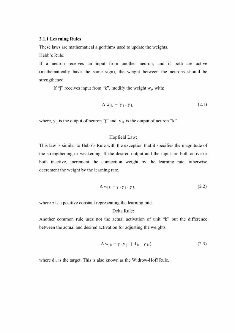
2.1.1 Learning Rules
These laws are mathematical algorithms used to update the weights.
Hebb’s Rule:
If a neuron receives an input from another neuron, and if both are active
(mathematically have the same sign), the weight between the neurons should be
strengthened.
If “j” receives input from “k”, modify the weight wjk with:
∆ wj k = y j . y k (2.1)
where, y j is the output of neuron “j” and y k is the output of neuron “k”.
Hopfield Law:
This law is similar to Hebb’s Rule with the exception that it specifies the magnitude of
the strengthening or weakening. If the desired output and the input are both active or
both inactive, increment the connection weight by the learning rate, otherwise
decrement the weight by the learning rate.
∆ wj k = γ . y j . y k (2.2)
where γ is a positive constant representing the learning rate.
Delta Rule:
Another common rule uses not the actual activation of unit “k” but the difference
between the actual and desired activation for adjusting the weights.
∆ wj k = γ . y j . ( d k – y k ) (2.3)
where d k is the target. This is also known as the Widrow-Hoff Rule.

2.1.2 Learning Algorithms
Forwardpropagation:
Forwardpropagation is a supervised learning algorithm and describes the "flow
of information" through a neural network from its input layer to its output layer.
The algorithm works as follows:
1. Set all weights to random values ranging from -1.0 to +1.0
2. Set an input pattern (binary values) to the neurons of the net's input layer
3. Activate each neuron of the following layer:
4. Multiply the weight values of the connections leading to this neuron with the
output values of the preceding neurons
5. Add up these values
6. Pass the result to an activation function, which computes the output value of
this neuron
7. Repeat this until the output layer is reached
8. Compare the calculated output pattern to the desired target pattern and
compute an error value
9. Change all weights by adding the error value to the (old) weight values
10. Go to step 2
11. The algorithm ends, if all output patterns match their target patterns
Backpropagation:
Backpropagation is a supervised learning algorithm and is mainly used by Multi
Layer-Perceptrons to change the weights connected to the net's hidden neuron layer(s).
The backpropagation algorithm uses a computed output error to change the weight
values in backward direction.
To get this network error, a forwardpropagation phase must have been done before.
While propagating in forward direction, the neurons are being activated using the
sigmoid activation function.
The formulation of sigmoid activation is:
inputexf
−+=
11)(
(2.4)

The alg
e forwardpropagation phase for an input pattern and calculate the
. Change all weight values of each weight matrix using the formula
weight(new) = (n urons *
output(neurons i+1) * ( 1 - output(neurons i+1) )
5. The algorithm ends, if all output patterns match their target patterns
2.1.3 T
ers, while feedback
neurons of the same layer.
1) Perc
licated logical operations (like the XOR
ron.
2) Mult
utput layers. It is mainly used in complex logical operations and pattern
3) Recu
and output neurons. The main
pplication is the storage and recognition of patterns.
orithm works as follows:
1. Perform th
output error
2
weight(old) + learning rate * output error * output e i)
4. Go to step 1
ypes of Neural Networks
There are several types of neural networks exist. They can be distinguished by
their type or their structure and the learning algorithm they use. Feedforward neural
networks allow only neuron connections between two different lay
networks have also connections between
eptron (Single Layer Networks):
It is a very simple neural network type with two neuron layers that accepts only
binary input and output values (0 or 1). The learning process is supervised and the
network is able to solve basic logical operations like “AND” or “OR”. It is also used for
pattern classification purposes. More comp
problem) can not be solved by a Percept
i Layer Feedforward Networks:
It is an extended Perceptron and has one ore more hidden neuron layers between
its input and o
classification.
rsive Networks:
They consist of a set of neurons, where each neuron is connected to every other
neuron. There is no differentiation between input
a
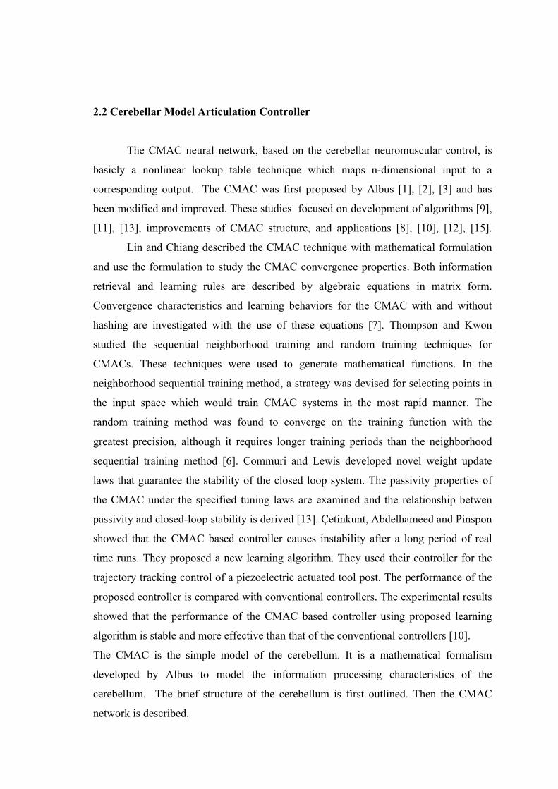
2.2 Cerebellar Model Articulation Controller
ing
structure of the cerebellum is first outlined. Then the CMAC
etwork is described.
The CMAC neural network, based on the cerebellar neuromuscular control, is
basicly a nonlinear lookup table technique which maps n-dimensional input to a
corresponding output. The CMAC was first proposed by Albus [1], [2], [3] and has
been modified and improved. These studies focused on development of algorithms [9],
[11], [13], improvements of CMAC structure, and applications [8], [10], [12], [15].
Lin and Chiang described the CMAC technique with mathematical formulation
and use the formulation to study the CMAC convergence properties. Both information
retrieval and learning rules are described by algebraic equations in matrix form.
Convergence characteristics and learning behaviors for the CMAC with and without
hashing are investigated with the use of these equations [7]. Thompson and Kwon
studied the sequential neighborhood training and random training techniques for
CMACs. These techniques were used to generate mathematical functions. In the
neighborhood sequential training method, a strategy was devised for selecting points in
the input space which would train CMAC systems in the most rapid manner. The
random training method was found to converge on the training function with the
greatest precision, although it requires longer training periods than the neighborhood
sequential training method [6]. Commuri and Lewis developed novel weight update
laws that guarantee the stability of the closed loop system. The passivity properties of
the CMAC under the specified tuning laws are examined and the relationship betwen
passivity and closed-loop stability is derived [13]. Çetinkunt, Abdelhameed and Pinspon
showed that the CMAC based controller causes instability after a long period of real
time runs. They proposed a new learning algorithm. They used their controller for the
trajectory tracking control of a piezoelectric actuated tool post. The performance of the
proposed controller is compared with conventional controllers. The experimental results
showed that the performance of the CMAC based controller using proposed learn
algorithm is stable and more effective than that of the conventional controllers [10].
The CMAC is the simple model of the cerebellum. It is a mathematical formalism
developed by Albus to model the information processing characteristics of the
cerebellum. The brief
n

.2.1 The Cerebellum
tline of the structure and the function of the cerebellar cortex is
shown
otor outputs. Each of mossy fibers makes excitatory
(+) contact with granule cells [1].
2
This section explains how the information process is achieved in the cerebellum
of humans and other mammals. The cerebellum is attached to the midbrain and nestles
under the visual cortex as shown in Figure 2.4. It is involved with control of movements
of the body. Injury to the cerebellum results in movement disability such as overshoot in
reaching for objects and lack of coordination. During 1960s, the functional
interconnections between the principal components of in the cerebellar cortex are
identified. A brief ou
in Figure 2.5.
The principal input to the cerebellar cortex arrives by mossy fibers. Mossy fibers
carry information from different sources such as the vestibular system (balance), the
reticular information (alerting), the cerebral cortex (sensory motor activity), and sensor
organs that measure such quantities as position of joints, tension in tendons, velocity of
contraction of muscles, and pressure on skin. Mossy fibers can be categorized into two
classes based on their point of origin: those carrying information that may include
commands from higher levels in the motor system, and those carrying feedback
information about the results of m
Figure 2.4 Exterior view of human brain [21]
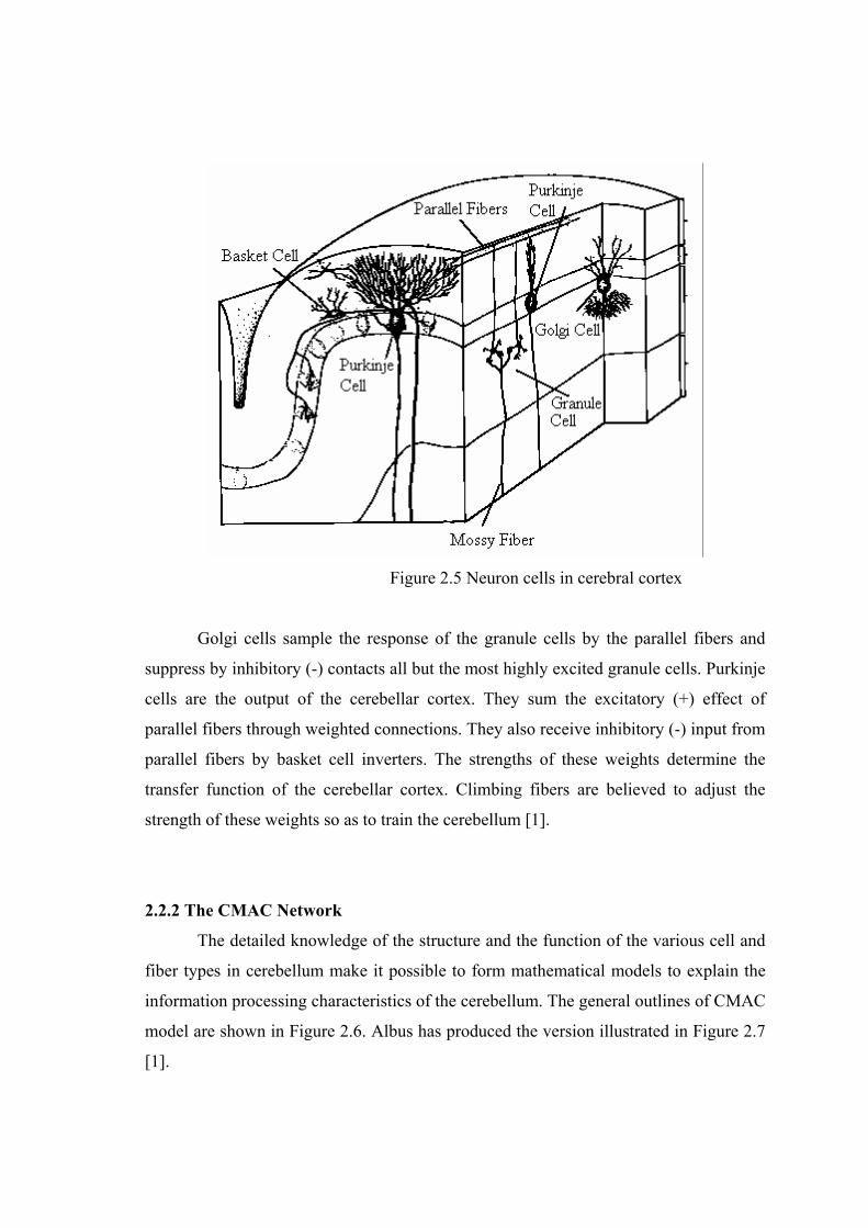
Figure 2.5 Neuron cells in cerebral cortex
Golgi cells sample the response of the granule cells by the parallel fibers and
suppress by inhibitory (-) contacts all but the most highly excited granule cells. Purkinje
cells are the output of the cerebellar cortex. They sum the excitatory (+) effect of
parallel fibers through weighted connections. They also receive inhibitory (-) input from
parallel fibers by basket cell inverters. The strengths of these weights determine the
transfer function of the cerebellar cortex. Climbing fibers are believed to adjust the
strength of these weights so as to train the cerebellum [1].
2.2.2 The CMAC Network
The detailed knowledge of the structure and the function of the various cell and
fiber types in cerebellum make it possible to form mathematical models to explain the
information processing characteristics of the cerebellum. The general outlines of CMAC
model are shown in Figure 2.6. Albus has produced the version illustrated in Figure 2.7
[1].

Figure 2.6 A Theoretical model of the cerebellum [1]
Figure 2.7 A schematic representation of CMAC [1]

The CMAC, as a controller, computes control values by referring to a memory
look-up table where those control values are stored [2]. Memory table basically stores
the relationship between input and output or the control function. In comparison to other
neural networks, CMAC has the advantage of very fast learning and it has the unique
property of quickly training certain areas of memory without affecting the whole
memory structure.
The network architecture of the CMAC is illustrated in Figure 2.8. The input
data of every state variable are quantized into discrete regions and mapped on to
different memory areas. Each indexed block memory called hypercube contains the
input data of one quantized discrete state. The association memory mapping is
implemented through hypercube to the actual memory as the mapping function of table
look-up model. In addition to the association memory mapping function, the CMAC
gives the feedback of the error of output to adjust the actual memory contents [1].
Figure 2.8 The learning architecture of CMAC
The output of this system is the summation of the contents of actual memory
that is mapped by effective hypercubes. The error caused by the difference between the
output summation and the desired output is processed as the feedback value for
adjusting the contents of actual memory. The learning efficiency of CMAC system

depends largely on the division of hypercube. Its technique can be explained with
Figure 2.9. This example has two state variables (s1 and s2) with each quantized into
four discrete regions, called blocks. For instance, s1 can be divided into A, B, C and D
and s2 can be divided into a, b, c and d. Areas formed by quantized regions, named as
Bb, Gg, Kk, Oo are called hypercubes in the input state of (s1, s2) = (7,7). If the
quantization for each variable is shifted by one element, different hypercubes will be
obtained. For example, E, F, G, H for s1 and e, f, g, h for s2 are shifted regions. Ee, Ff,
etc. are new hypercubes from the shifted regions. Each state is covered by N e different
hypercubes, where N e is the number of elements in a complete block. There are 64 ( =
42 x 4 ) hypercubes in this example. Each hypercube is taken as the corresponding
address of actual memory element. And the data of each state will be distributively
stored in memory elements associated with hypercubes that cover this state. Assume a j
represents an association vector of j th input space ( j = 1, 2,3 ... N s ) where N s indicates
the total number of input states. 99 th input state (state (7, 7)) is used to explain the
actual memory how to be mapped by an association memory. Figure 2.9 shows the state
(7,7) is mapped by the hypercubes of Bb,Gg,Kk and Oo. If we give an index value for
each mapped actual memory unit, then the state (7,7) can be mapped to the memory
locations of 6,27,43 and 59. We can use an association vector shown as equation 2.6 to
represent the mapping information.
a 6 a 27 a 43 a 59
a 99 = [ 0 . . . 0 1 0 . . . 0 1 0 . . . 0 1 0 . . . 0 1 0 . . .0 ] 1 x 64 (2.5)
Bb Gg Kk Oo
This is a 1×64 vector because there are 64 hypercubes needed (i.e. 64 actual
memory units are used) in this case. In this vector, four 1’s represent the mapped actual
memory units that are used under this input state, and other 0’s represent the mapped
actual memory units are not used. Therefore, the locations of 6,27,43 and 59 are
recorded as 1 and everything else is recorded as 0. The actual output y 99 of input state
(7,7) can be represented as:
y 99 = a 99 . w (2.6)
where w indicates the weight vector of actual memory contents.

Figure 2.9 Block division of CMAC for a two-variable example
Since there are total of 169(=13x13) input states in this case, the association
memory matrix can be represented as a 64 x 169 matrix shown as A matrix in equation
2.7. If we consider all corresponding outputs of input states, then the actual outputs can
be represented as:
y = A . W = (2.7)
116964
2
1
16464
2
1
64169169
2
1
...
xxxy
yy
W
WW
a
aa
⎥⎥⎥⎥
⎦
⎤
⎢⎢⎢⎢
⎣
⎡
=
⎥⎥⎥⎥
⎦
⎤
⎢⎢⎢⎢
⎣
⎡
⎥⎥⎥⎥
⎦
⎤
⎢⎢⎢⎢
⎣
⎡
where y indicates the vector of actual output, A indicates the association matrix and w
indicates the weight vector of actual memory. CMAC requires 10816 (= 169 x 64)
association memory units to record the information and requires 64 (= 64 x 1) actual
memory units to record the weight information on this case.

Every step of CMAC operation is defined in Chapter 3. Chapter 3 is also a guide
for writing a CMAC code in MATLAB environment.

CHAPTER 3
CMAC PROGRAMMING
This chapter includes programming details of the CMAC in the MATLAB
environment and function approximation examples in order to analyze the effects of the
CMAC parameters to the learning and learning convergence. There are not so much
detailed explanations about CMAC programming in the literature. Authors who studied
CMAC, preferred to explain the network structure based on mathematical neural form.
From another point of view the CMAC is a look-up table as well. And during the
programming phase, this perspective is useful to better understand the inner mechanism
of this network
3.1. The CMAC Mapping
The input space is quantized into a number of intervals according to the
generalization width. The distance among the input dimension of each interval is equal
to the generalization width. Quantized region of the input space is called a layer. New
layers can be added by shifting the intervals as shown in Figure 3.1, which is an
example for one-dimensional CMAC.
.
Figure 3.1 An example for quantized layers of the input space

The input space is defined between –5 and 14, the generalization width is equal
to 5 and there are four layers. Each layer can be modeled as a vector by shifting such as;
Layer 1 L1 = [ -5 0 5 10 ], Layer 3 L3 = [ -5 -3 2 7 12 ],
Layer 2 L2 = [ -5 -4 1 6 11 ], Layer 4 L4 = [ -5 -2 3 8 13 ].
A, B, C ... are the hypercubes that contain the weights. The hypercubes are
numbered as, “A = 1, B = 2, C = 3, ... , T = 19” and the CMAC memory is formed from
19 memory locations. An address function is needed to map the input values into the
memory locations.
The function, MAX ( FIND ( L i ≥ x ) ) where “MAX” and “FIND” are the
MATLAB commands, gives the hypercube number in the ith layer. For example, for the
input x = 3, in the first layer, 3 ≥ -5 and 3 ≥ 0. The command, find ( L1 ≥ 3 ) gives the
vector [ 1 2 ] and max ( [ 1 2 ] ) is equal to “2”. It means that the input x = 3, activates
the 2nd hypercube “B” in the first layer and similarly G, L and R in the other layers as
seen in Figure 3.2.
Figure 3.2 Single point mapping for one-dimensional CMAC.
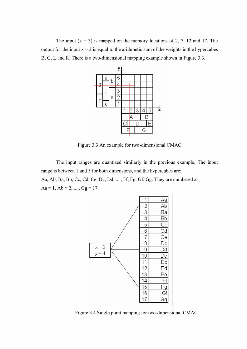
The input (x = 3) is mapped on the memory locations of 2, 7, 12 and 17. The
output for the input x = 3 is equal to the arithmetic sum of the weights in the hypercubes
B, G, L and R. There is a two-dimensional mapping example shown in Figure 3.3.
Figure 3.3 An example for two-dimensional CMAC
The input ranges are quantized similarly in the previous example. The input
range is between 1 and 5 for both dimensions, and the hypercubes are;
Aa, Ab, Ba, Bb, Cc, Cd, Ce, Dc, Dd, ... , Ff, Fg, Gf, Gg. They are numbered as;
Aa = 1, Ab = 2, ... , Gg = 17.
Figure 3.4 Single point mapping for two-dimensional CMAC.
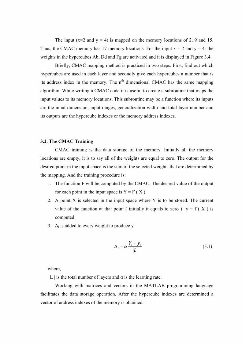
The input (x=2 and y = 4) is mapped on the memory locations of 2, 9 and 15.
Thus, the CMAC memory has 17 memory locations. For the input x = 2 and y = 4: the
weights in the hypercubes Ab, Dd and Fg are activated and it is displayed in Figure 3.4.
Briefly, CMAC mapping method is practiced in two steps. First, find out which
hypercubes are used in each layer and secondly give each hypercubes a number that is
its address index in the memory. The nth dimensional CMAC has the same mapping
algorithm. While writing a CMAC code it is useful to create a subroutine that maps the
input values to its memory locations. This subroutine may be a function where its inputs
are the input dimension, input ranges, generalization width and total layer number and
its outputs are the hypercube indexes or the memory address indexes.
3.2. The CMAC Training
CMAC training is the data storage of the memory. Initially all the memory
locations are empty, it is to say all of the weights are equal to zero. The output for the
desired point in the input space is the sum of the selected weights that are determined by
the mapping. And the training procedure is:
1. The function F will be computed by the CMAC. The desired value of the output
for each point in the input space is Y = F ( X ).
2. A point X is selected in the input space where Y is to be stored. The current
value of the function at that point ( initially it equals to zero ) y = f ( X ) is
computed.
3. ∆i is added to every weight to produce yi
LyY ii
i−
=∆ α (3.1)
where,
| L | is the total number of layers and α is the learning rate.
Working with matrices and vectors in the MATLAB programming language
facilitates the data storage operation. After the hypercube indexes are determined a
vector of address indexes of the memory is obtained.

For the ith training point, the output is Y( i ) = sum ( M ( address ( : ) ) ) where,
“M” is the memory vector and “address” is the vector of the address indexes and
M ( address ( : ) ) = M ( address ( : ) ) + α ( Y ( i ) – y ( i ) ) / A.
After all the points in the input space are trained, this loop is repeated for the same
points until the memory elements converge.
There are three cases:
1. Memory elements change periodically after a cycle.
2. Memory elements remain constant after a cycle.
3. Instability.
Convergence is gained in two ways. The memory elements remain constant after a
certain cycle or the memory elements have the same values periodically. In which cycle,
the elements converge, depends on the CMAC parameters, selected training points and
the chosen size of the memory. If there are no learning interferences between the
training points and if hash coding is not used, the memory elements converge at the first
cycles. Very high learning rates may result in instability while very low learning results
cause long convergence time. By using adaptive learning algorithms, the instability
problem is solved [9].
Here the CMAC operation is described by using the Figure 2.9. Figure 2.9
displays a two dimensional CMAC. For instance, the input pairs are s1 = 7 and s2 = 7
and the target value t = 4. The input pairs s1 and s2 will activate the weigths in the
hypercubes Bb, Gg, Kk and Oo. There are 64 hypercubes in this example and the index
numbers of Bb, Gg, Kk and Oo 6, 27, 43 and 59. After the first training the sum of these
four weights in the hypercubes Bb, Gg, Kk and Oo will be equal to 4. Initially all the
weights are equal to zero. So, each weight in these hypercubes will be equal to 1 in
order to give the output 4.
For example, after the first training, to calculate the output for the input pairs s1 = 7 and
s2 = 8 first the active weights must be found. These are Bc, Gg, Kk and Oo. The
memory index of Bc is 7. The weight value in Bc was not active in the training so it
remained zero. The output for s1 = 7 and s2 = 8 will be equal to the sum of the weights
in Bc, Gg, Kk and Oo. Gg, Kk and Oo are equal to 1 and Bc is equal to so the output is
equal to 3.

3.3. Hash Coding
As the dimension of the CMAC network increases, the required size of the
CMAC memory increases exponentionally. After CMAC mapping, mapping the
indexes into a smaller memory rather than the CMAC memory is a solution for the case
of large memory requirements. Hash coding is used to solve this problem. The main
idea is:
index CMAC MAPPING = MOD (index HASH MAPPING , hash size) (3.2)
Formulation 3.2 causes different data mapped in the same memory address. This
is called hash collisions. But usually, the errors due to the hash collisions are neglected
with respect to the overall CMAC error. And choosing an appropriate hash size is
important to minimize the errors due to the hash coding. One that gives smooth results
is formulated below:
∏=
⎟⎠⎞
⎜⎝⎛ +=
n
i
i
wI
ks1
1 (3.3)
where,
s : hash size
I : input range
w : generalization width
n : input dimension
k = 1,2,3, …
Formulation 3.3 is used in the case of no learning interferences and it is
displayed in Figure 3.5 for one-dimensional and in Figure 3.6 for two-dimensional input
spaces. This basic sense can be applied for the n-dimensional input space. Here, the
distance between two consecutive training points is equal to the generalization width.
The training points are selected in this fashion.
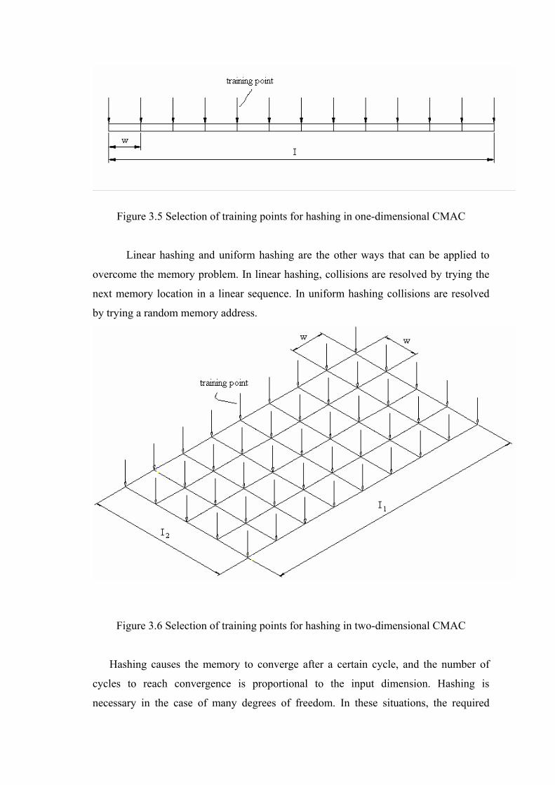
Figure 3.5 Selection of training points for hashing in one-dimensional CMAC
Linear hashing and uniform hashing are the other ways that can be applied to
overcome the memory problem. In linear hashing, collisions are resolved by trying the
next memory location in a linear sequence. In uniform hashing collisions are resolved
by trying a random memory address.
Figure 3.6 Selection of training points for hashing in two-dimensional CMAC
Hashing causes the memory to converge after a certain cycle, and the number of
cycles to reach convergence is proportional to the input dimension. Hashing is
necessary in the case of many degrees of freedom. In these situations, the required

memory with CMAC mapping may not be possible physically so hash coding is a must
to solve this problem. During this study the hardware implementation is performed with
the PC interface and the PC RAM is used for the CMAC memory. For the limited sized
memory devices such as micro controllers, the hash coding algorithms help to use the
memory capacity economically.
3.3. Function Approximation with the CMAC
CMAC is a good function approximator for both single and multi input
functions. Albus, proposed CMAC to determine the control function of a robotic
motion. Especially for the many degrees of freedom, it is hard to solve the analytic
equations and sometimes it is not possible to model the physical properties of
interactions like friction. Although all the terms of the equations of the motion are
exactly found, solving these equations may not be so practical. Rather than kinematic
solutions, referring to a table the output is calculated for the desired input values.
Actually, CMAC determines the same equations of the motion by learning in an
adaptive manner without any knowledge of the physical laws. That’s what the human
and the other mammals do while acting their motions. Some points in the input space is
trained during training but by using the generalization property of the CMAC, the
network gives output for every input point in the input range. This is the basic result of
the idea “the similar inputs give similar outputs”. Mathematically, generalization
property is suitable to approximate to the continuous functions like motion control
functions. If the generalization width is taken one, then the CMAC look- up table
becomes a simple look-up table and the outputs of the points rather than the trained
points remain zero. If the generalization width is too large, some overlaps will be
formed. This overlaps causes the network to converge after many cycles and finally
with an unacceptable error. If the generalization width is chosen approximately equal to
the distance between the training points of the input space, a function with an acceptable
error is obtained. Another parameter of the CMAC is the total number of layers. As the
number of layers increases, output becomes more precise because more weights are
used for output calculation since the number of weights is exactly equal to the number
of layers used. Networks with more layers need more memory locations. Generalization
width, number of layers, training point numbers are the key parameters for the function
approximation. There is no criteria or formulation to optimize these parameters. Some
examples are shown here to see how the approximation changes with the parameters.
These examples give an idea for the network architecture.
The sine function { y = sin ( x ), -180≤ x ≤ 180 } is used as an example for the
CMAC approximation. In the below tables, the output of the CMAC and the target
function are plotted in the first figure. Next figure represents the convergence of the
network.
The CMAC parameters like total layer number, generalization width, learning
rate and training points are stated. The maximum error and the mean error of the CMAC
output are calculated. Some graphs are introduced for optimum parameters.
In Table 3.1 total number of layers is equal to 10 and the generalization width is
equal to 30. {-180, -150, -120, -90, -60, -30, 0, 30, 60, 90, 180} are the training points.
130 memory locations are required and there is no hashing. The memory converges
after the second cycle as seen in Figure 3.7.2 and the memory elements take the same
values at every two cycles periodically. The learning rate is equal to 1 and remains
constant during learning. The maximum error is 0.3084 and the mean error is 0.0917.
Approximation results for this example are under the desired performance level.
The training points’ set, {-180, -150, -120, -90, -60, -30, 0, 30, 60, 90, 180} is
represented in a MATLAB vector form as (-180 : 30 : 180) . In the memory
convergence graph the vertical axis defines the sum of the memory elements. As it is
mentioned before in this chapter, the convergence is obtained in two ways: the memory
elements remain constant after a certain cycle or take the same values periodically after
a certain cycle. In Figure 3.7.2 it is seen that the memory convergence like in the second
way.

Figure 3.7.1 Sine approximation
Figure 3.7.2 Memory Convergence
L W α Training points Maximum Error Mean Error
10 30 1 (-180 : 30 : 180) 0.3084 0.0917
Required Memory Locations Hash Size Convergence
130 No hashing Periodical
Table 3.1 CMAC parameters and sine approximation results
Figure 3.8.1 Sine approximation
Figure 3.8.2 Memory Convergence
L W α Training points Maximum Error Mean Error
30 30 1 (-180 : 30 : 180) 0.0329 0.0146
Required Memory Locations Hash Size Convergence
390 No hashing Periodical
Table 3.2 CMAC parameters and sine approximation results

In Table 3.2 the total number of layers is increased from 10 to 30 so the required
memory locations are increased from 130 to 390. There is no hashing. The same points
in the input space are used for training (-180:30:180). The maximum error is decreased
from 0.3084 to 0.0329 and the mean error decreased from 0.0917 to 0.0146. After
convergence is obtained, the memory elements take the same values for every 10 cycles
periodically.
It is clear that the approximation is better than the previous one in Table 3.1.
While the training points and the generalization width are the same with the example in
Table 3.1, the total number of layers is increased from 10 to 30 and a better
approximation is gained. Also it is seen that more memory locations are needed as the
convergence characteristic of the memory is changed. So, the total number of layers
affects the approximation performance and it has a direct effect on the memory.
The total layer number and the maximum error relations are seen in Figure 3.9
and the total layer number and mean error relations are seen in Figure 3.10. Other
parameters are the same with the examples in Table 3.1 and Table 3.2. Training points
are (-180:30:180), without hashing. The generalization width is 30 and learning rate is
equal to 1.
Figure 3.9 Maximum error – total number of layers. (w=30)
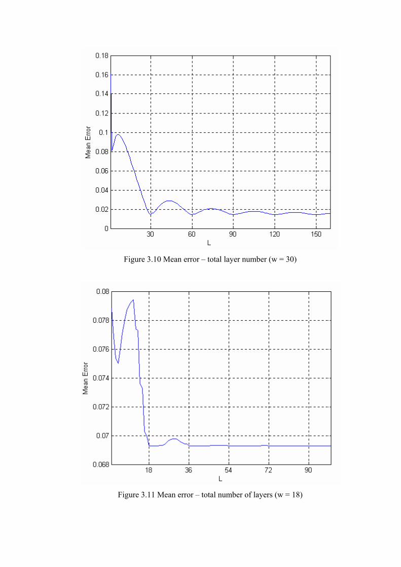
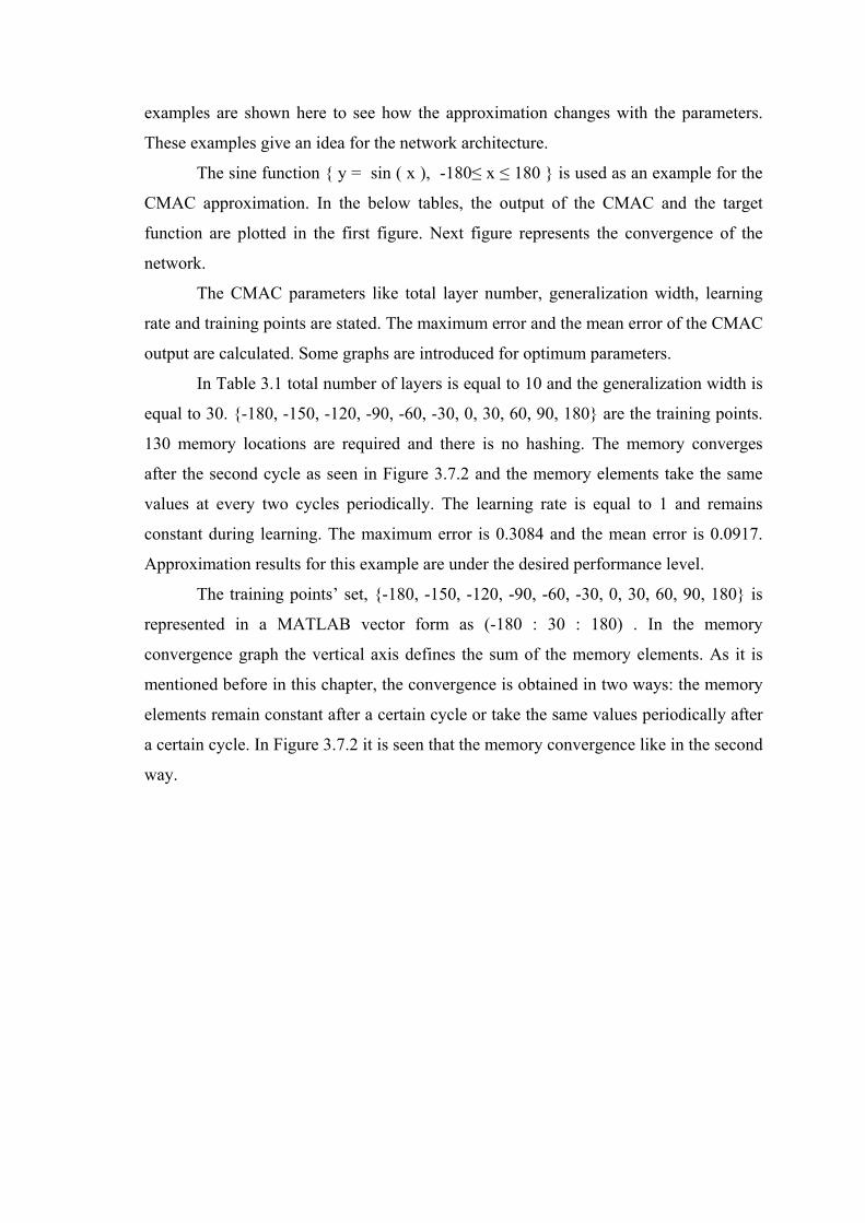
Figure 3.10 Mean error – total layer number (w = 30)
Figure 3.11 Mean error – total number of layers (w = 18)

It is clear that for L < 30, error values are high and the minimum points are
periodically at 30, 60, 90, 120, 150, … that are the multiples of 30.
Approximately,
L ≈ k . w (3.4)
where, k = 1,2,3, ...
The maximum error and minimum error are similarly affected with the total
number of layers. In Figure 3.11 the same experiment was performed with 21 training
points with no learning interference and where generalization width equals to 18. Figure
3.11 displays the relation of the mean error and total number of layers. The minimum
error values are at points where total number of layers is equal to 18 and its multiples.
Choosing low L, is an advantage for less memory and fast computation and fast
convergence. How many training points are used and training point locations affect the
generalization width. And it is seen that the generalization width affects the total
number of layers. And taking total number of layers equal to generalization width seems
to be an optimum selection.
Figure 3.12.1 Sine approximation
Figure 3.12.2 Memory Convergence
L w α Training points Maximum Error Mean Error
36 36 1 (-180 : 30 : 180) 0.1263 0.0660
Required Memory Locations Hash Size Convergence
396 No hashing Constant
Table 3.3 CMAC parameters and sine approximation results
In table 3.3 the generalization width and the total number of layers are equal to
36. 396 memory locations are required and there is no hashing. The convergence is

obtained after 6 cycles and the memory elements remain at constant values as seen in
Figure 3.12.2. The maximum error is 0.1263 and the mean error is 0.0660. The same
training points (-180 : 30 : 180 ) are used for training and it is seen that the error values
are increased by increasing generalization width and total number of layers. In Table 3.3
by increasing the generalization width with constant training points, learning
interferences form. Also by increasing training data with constant generalization width
causes learning interferences. In Figure 3.12.1 it is seen that with increasing
generalization width the error values also increase. Figure 3.13 and 3.14 show the
relations between the error values and the generalization width. In these graphs the
generalization width values are equal to the total number of layers. Each error value is
calculated after convergence. Optimum results are obtained when w = 30. For w < 30
there are no learning interferences, but there are untrained gaps between two training
points so the learning is insufficient. w = 30 is a boundary for learning interference. The
mean error doesn’t change dramatically for w > 30 but it is clear to choose w = 30 if the
maximum error is taken into account.
Figure 3.13 Mean error – total number of layers, generalization width
training points ( –180 : 30 :180 )
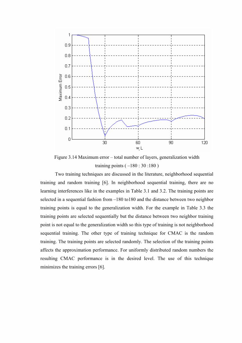
Figure 3.14 Maximum error – total number of layers, generalization width
training points ( –180 : 30 :180 )
Two training techniques are discussed in the literature, neighborhood sequential
training and random training [6]. In neighborhood sequential training, there are no
learning interferences like in the examples in Table 3.1 and 3.2. The training points are
selected in a sequential fashion from –180 to180 and the distance between two neighbor
training points is equal to the generalization width. For the example in Table 3.3 the
training points are selected sequentially but the distance between two neighbor training
point is not equal to the generalization width so this type of training is not neighborhood
sequential training. The other type of training technique for CMAC is the random
training. The training points are selected randomly. The selection of the training points
affects the approximation performance. For uniformly distributed random numbers the
resulting CMAC performance is in the desired level. The use of this technique
minimizes the training errors [6].
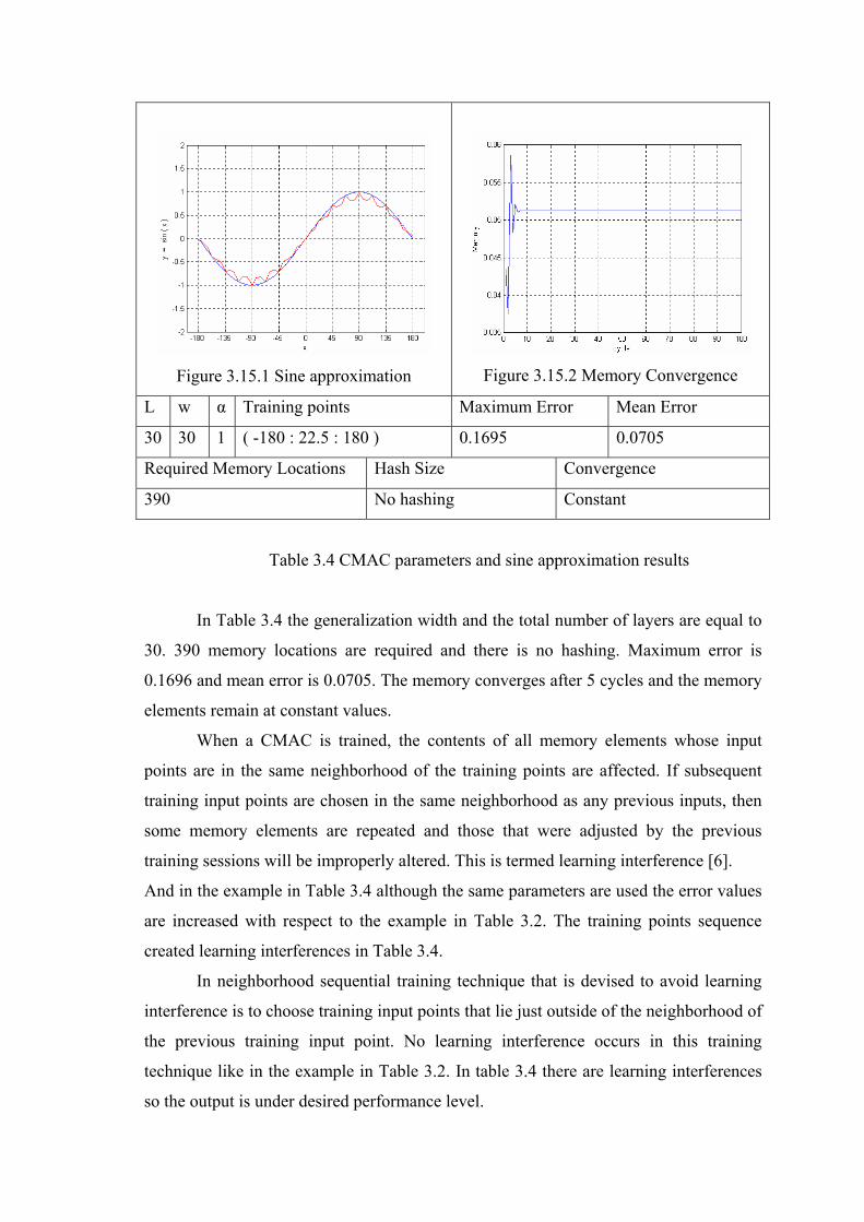
Figure 3.15.1 Sine approximation
Figure 3.15.2 Memory Convergence
L w α Training points Maximum Error Mean Error
30 30 1 ( -180 : 22.5 : 180 ) 0.1695 0.0705
Required Memory Locations Hash Size Convergence
390 No hashing Constant
Table 3.4 CMAC parameters and sine approximation results
In Table 3.4 the generalization width and the total number of layers are equal to
30. 390 memory locations are required and there is no hashing. Maximum error is
0.1696 and mean error is 0.0705. The memory converges after 5 cycles and the memory
elements remain at constant values.
When a CMAC is trained, the contents of all memory elements whose input
points are in the same neighborhood of the training points are affected. If subsequent
training input points are chosen in the same neighborhood as any previous inputs, then
some memory elements are repeated and those that were adjusted by the previous
training sessions will be improperly altered. This is termed learning interference [6].
And in the example in Table 3.4 although the same parameters are used the error values
are increased with respect to the example in Table 3.2. The training points sequence
created learning interferences in Table 3.4.
In neighborhood sequential training technique that is devised to avoid learning
interference is to choose training input points that lie just outside of the neighborhood of
the previous training input point. No learning interference occurs in this training
technique like in the example in Table 3.2. In table 3.4 there are learning interferences
so the output is under desired performance level.

In Table 3.5 the sequential neighborhood training technique is used and the
output performance level is higher than the previous example. The generalization width
and the total number of layers are equal to 15. 375 memory locations are required and
there is no hashing. The memory converges after 2 cycles. The maximum error is
0.0084 and the mean error is 0.0036.
Figure 3.17.1 Sine approximation
Figure 3.17.2 Memory Convergence
L w α Training points Maximum Error Mean Error
15 15 1 ( -180 : 15 : 180 ) 0.0084 0.0036
Required Memory Locations Hash Size Convergence
375 No hashing Periodical
Table 3.5 CMAC parameters and sine approximation results
There are more training points in the example in Table 3.5 ( -180 : 15 : 180 ) and
the approximation performance is higher than the example in Table 3.2 ( -180 : 30 :
180).
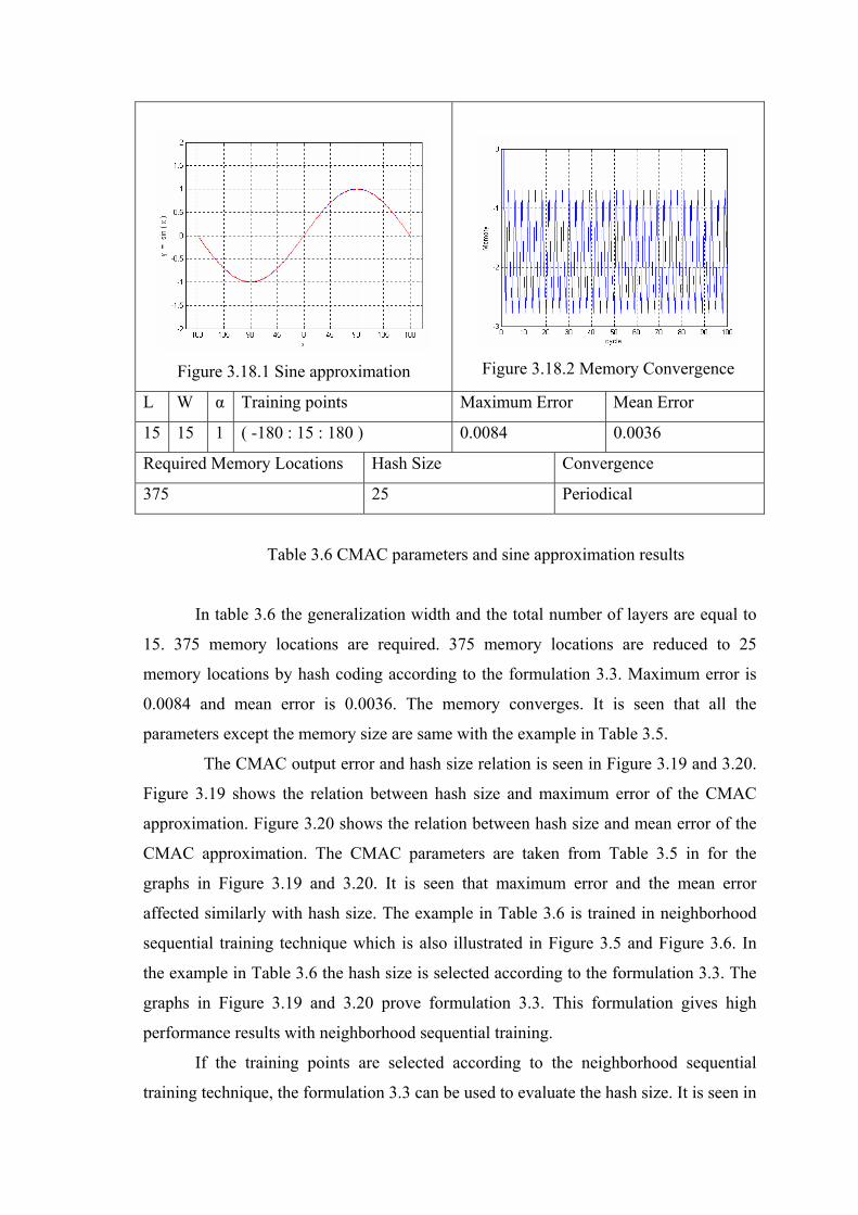
Figure 3.18.1 Sine approximation
Figure 3.18.2 Memory Convergence
L W α Training points Maximum Error Mean Error
15 15 1 ( -180 : 15 : 180 ) 0.0084 0.0036
Required Memory Locations Hash Size Convergence
375 25 Periodical
Table 3.6 CMAC parameters and sine approximation results
In table 3.6 the generalization width and the total number of layers are equal to
15. 375 memory locations are required. 375 memory locations are reduced to 25
memory locations by hash coding according to the formulation 3.3. Maximum error is
0.0084 and mean error is 0.0036. The memory converges. It is seen that all the
parameters except the memory size are same with the example in Table 3.5.
The CMAC output error and hash size relation is seen in Figure 3.19 and 3.20.
Figure 3.19 shows the relation between hash size and maximum error of the CMAC
approximation. Figure 3.20 shows the relation between hash size and mean error of the
CMAC approximation. The CMAC parameters are taken from Table 3.5 in for the
graphs in Figure 3.19 and 3.20. It is seen that maximum error and the mean error
affected similarly with hash size. The example in Table 3.6 is trained in neighborhood
sequential training technique which is also illustrated in Figure 3.5 and Figure 3.6. In
the example in Table 3.6 the hash size is selected according to the formulation 3.3. The
graphs in Figure 3.19 and 3.20 prove formulation 3.3. This formulation gives high
performance results with neighborhood sequential training.
If the training points are selected according to the neighborhood sequential
training technique, the formulation 3.3 can be used to evaluate the hash size. It is seen in

the graphs in Figure 3.19 and 3.20 good results are obtained at 25 and its multiples. In
this example the required memory locations are reduced to 25 from 375 and the
performance of the approximation did not changed in sine approximation example. In
the case of multi-dimensional CMAC networks hashing is very useful to use less
memory space. But in this hashing algorithm the training points and hash size must be
selected very carefully else the error values increases as shown in the graphs in Figure
3.19 and 3.20. For instance if the hash size is 150 the mean error is approximately 0.004
while mean error is over 0.6 if the hash size is 188.
Figure 3.19 Hash size – maximum error
One dimensional function approximation of CMAC
where training points set (-180 : 15 : 180) and L = 15, w = 15

Figure 3.20 Hash size – mean error
One dimensional function approximation of CMAC
where training points set (-180 : 15 : 180) and L = 15, w = 15
In the example in Table 3.7 the training points are selected randomly at 43
points. Total number of layers and generalization width is 55. The learning rate is equal
to 1. 415 memory locations are required and there is no hashing. Memory converges
after 100 cycles and the memory elements remain at constant values. Maximum error is
0.0861 and mean error is 0.0189. It is seen that in graph in Figure 3.211 there are
untrained regions between points –135 and –90 and between 75 and 105. The training
point set for this example is {-143 -126 70 14 107 97 -114 129 -65 31 -175 -66 -127 85
7 -140 32 104 162 -116 -165 -128 -79 87 17 66 -73 -68 24 -12 -55 -39 -33 -10 -44 -3 -
94 111 30 -164 40 28 125}.
In the random training technique the convergence is gained after more cycles
with respect to neighborhood sequential training technique. In the example in Table
3.20 the convergence is gained after 100 cycles while the convergence is gained in the
first cycle in neighborhood sequential training technique. But the training point
distribution is very important in random training technique. If there are no untrained
gaps in the input space by the help of generalization the learning errors are minimized

after cycles while in the neighborhood training technique the learning errors do not
change with cycles.
Figure 3.21.1 Sine approximation
Figure 3.21.2 Memory Convergence
L w α Training points Maximum Error Mean Error
55 55 1 Random 43 points 0.0861 0.0189
Required Memory Locations Hash Size Convergence
415 No hashing Constant
Table 3.7 CMAC parameters and sine approximation results
Figure 3.22 shows the relation between the total number of layers and CMAC
output mean error. The CMAC parameters are equal to the parameters in the example in
Table 3.7. Figure 3.10 shows that the total number of layers is affected with the
generalization width. This relation is valid for neighborhood sequential training
technique. In random training technique there is no such relationship. But in Figure 3.22
it is seen that the error values are low where total number of layers are higher than 20.
In Figure 3.23 and Figure 3.24 the generalization width changes with total
number of layers. It is seen that for very high and low values the maximum error is high
but the mean error does not change after a certain value where generalization width and
the total number of layers are equal to 60. But in Figure 3.23 the maximum error
increases with the increasing generalization width and total number of layers.
According to the total number of layers and the CMAC performance graphs, low
total number of layers results in unacceptable approximations. On the other hand very
high values of total number of layers cause high maximum errors. As a result,

convergence is slowed down. As the number of layers increases there are more loops in
the program code so this makes slower learning and output calculation.
Figure 3.22 Mean error – total number of layers
w = 55, random training in 43 points

Figure 3.23 Maximum error – total number of layers
random training in 43 points
Figure 3.24 Mean error – total number of layers
random training in 43 points

In Table 3.8 the generalization width and the total number of layers is 55. The
learning rate is equal to 1. The training points are randomly chosen and same with the
example in Table 3.7. 415 memory locations are required. It is reduced to 200 memory
locations by using hash coding. The maximum error is 0.0892 and mean error of the
output is 0.0211. Convergence is obtained after 250 cycles. The number of cycles to
reach the convergence is increased with hash coding. So it can be said that the random
training technique and hash coding cause the convergence to be reached after more
cycles than the situations with no hashing.
Generally, in neighborhood sequential training all memory elements are not
addressed during training because some memory elements are not modified and remain
zero. Hash size is reduced to very low values with respect to the required memory size
of CMAC. But there is no such a relationship in random training technique. And the
formulation 3.3 can not be used for estimating the hash size in the case of random
training. Other hashing algorithms rather than the one applied to neighborhood training
can be used for better approximation and low hash size values.
Figure 3.25.1 Sine approximation
Figure 3.25.2 Memory Convergence
L w Α Training points Maximum Error Mean Error
55 55 1 Random 43 points 0.0892 0.0211
Required Memory Locations Hash Size Convergence
415 200 Constant
Table 3.8 CMAC parameters and sine approximation results

Two-dimensional CMAC examples are seen in Figure 3.26 and Figure 3.28. (z =
sin ( x ) . cos (y ) ). In Figure 3.26 the CMAC parameters are;
w = 30, L = 30, α = 1, the sequential neighborhood training technique is used.
Results are:
Maximum Error = 0.0170, and mean error = 0.0056.
2510 memory locations are used.
Figure 3.26 the CMAC parameters are;
w = 15, L = 15, α = 1, the sequential neighborhood training technique is used.
Results are:
Maximum Error = 0.0669, and mean error = 0.0221.
1470 memory locations are hashed into 49 memory locations. The convergence
curves are seen in Figure 3.27 and 3.29. The hashing algorithm makes CMAC to
converge after a certain number of cycles. In case of no hashing like the example in
Figure 3.26 the memory elements convergence at the first cycle. But as it is seen in
Figure 3.29 the convergence is obtained after 250 cycles for the example in Figure 3.28.
But if the memory requirements are taken into account and the convergence speed is
less important than the memory capacity than hashing is very advantageous in that case.
Figure 3.26 CMAC output for approximation of the function z = sin ( x ) cos ( y)

Figure 3.27 Memory convergence of two-dimensional CMAC
Figure 3.28 CMAC output for approximation of the function z = sin ( x ) cos ( y)
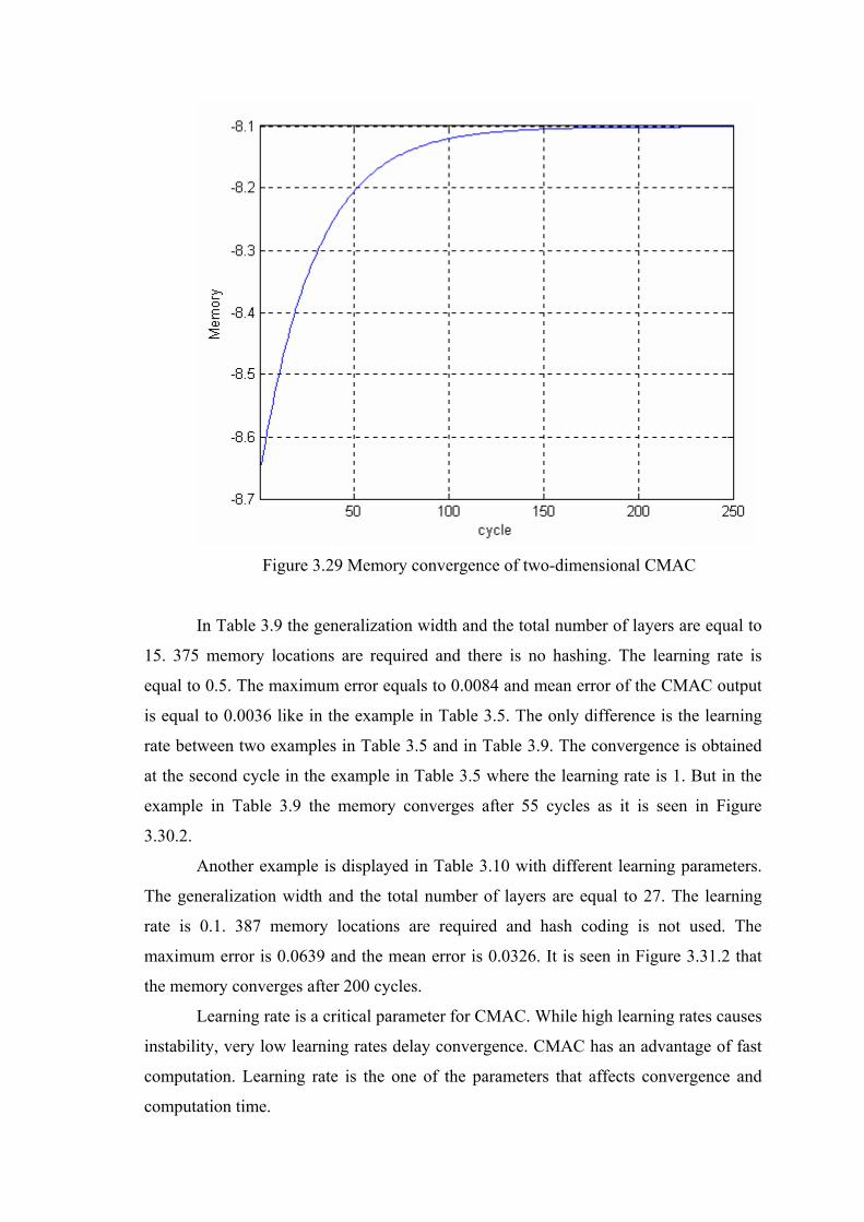
Figure 3.29 Memory convergence of two-dimensional CMAC
In Table 3.9 the generalization width and the total number of layers are equal to
15. 375 memory locations are required and there is no hashing. The learning rate is
equal to 0.5. The maximum error equals to 0.0084 and mean error of the CMAC output
is equal to 0.0036 like in the example in Table 3.5. The only difference is the learning
rate between two examples in Table 3.5 and in Table 3.9. The convergence is obtained
at the second cycle in the example in Table 3.5 where the learning rate is 1. But in the
example in Table 3.9 the memory converges after 55 cycles as it is seen in Figure
3.30.2.
Another example is displayed in Table 3.10 with different learning parameters.
The generalization width and the total number of layers are equal to 27. The learning
rate is 0.1. 387 memory locations are required and hash coding is not used. The
maximum error is 0.0639 and the mean error is 0.0326. It is seen in Figure 3.31.2 that
the memory converges after 200 cycles.
Learning rate is a critical parameter for CMAC. While high learning rates causes
instability, very low learning rates delay convergence. CMAC has an advantage of fast
computation. Learning rate is the one of the parameters that affects convergence and
computation time.

Figure 3.30.1 Sine approximation
Figure 3.30.2 Memory Convergence
L W α Training points Maximum Error Mean Error
15 15 0.5 ( -180 : 15 : 180 ) 0.0084 0.0036
Required Memory Locations Hash Size Convergence
375 No hashing Periodical
Table 3.9 CMAC parameters and sine approximation results
Figure 3.31.1 Sine approximation
Figure 3.31.2 Memory Convergence
L w α Training points Maximum Error Mean Error
27 27 0.1 ( -180 : 15 : 180 ) 0.0639 0.0326
Required Memory Locations Hash Size Convergence
387 No hashing Constant
Table 3.10 CMAC parameters and sine approximation results

In Table 3.11 the generalization width and the total number of layers are equal to
15387 memory locations are required without hashing. The learning rate is equal to 2
and remains constant during the learning. But as it is seen in Figure 3.32.1 the output
performance of the CMAC approximation is very low. The high learning rate causes
this situation. And the Figure 3.32.2 displays that the memory elements do not converge
still after 2500 cycles. The output of the CMAC changes for every training cycle and
never reaches to desired performance level.
In Table 3.12 the same CMAC parameters are used with the example in Table
3.11 but the learning rate is reduces from two to zero for every cycle. Finally after 50
cycles the memory converges and approximation is in the desired performance level.
It is seen that high learning rates cause instability. The memory contents of a
CMAC with or without hash coding will converge, provided that the learning rate
values lies between two and zero. Table 3.12 is an example for this case.
Figure 3.32.1 Sine approximation
Figure 3.32.2 Memory Convergence
L w α Training points Max error Mean Error
15 15 2 ( -180 : 15 : 180 ) Instability Instability
Required Memory Locations Hash Size Convergence
387 No hashing Doesn’t converge
Table 3.11 CMAC parameters and sine approximation results

Figure 3.31.1 Sine approximation
Figure 3.31.2 Memory Convergence
L w Α Training points Maximum Error Mean Error
15 15 2 → 0 ( -180 : 15 : 180 ) 0.0084 0.0036
Required Memory Locations Hash Size Convergence
387 No hashing Periodical
Table 3.12 CMAC parameters and sine approximation results

CHAPTER 4
ROBOTIC CONTROL WITH CMACs
The artificial neural networks theory made it possible to develop adaptive
solutions to complex control problems, such as inverse kinematics control for robotic
systems. In this chapter a CMAC network is used for the inverse kinematics control of a
two degrees of freedom serial manipulator. In the first section general concepts of the
robotic control are outlined. The second section explains the inverse kinematics
problem for the serial manipulators. The CMAC network and the control architectures
are presented with the simulation results in the third section. A hardware
implementation of two degrees of freedom serial manipulator is seen in the fourth
section.
4.1. Robotic Control
The task of the robotic control is separated into two groups as motion control
and force control. The motion control is a point to point control or continuous trajectory
control. The control scheme can be open loop or closed loop. Very few robots use
stepper motors or other actuators which can be controlled in an open fashion. Usually,
manipulators are powered by actuators which output a torque or a force at each joint
[20]. Figure 4.1 shows the basic idea of robotic control. Motion planning includes
trajectory generation and forward/inverse kinematics computation. A robot is composed
of joint motors, breaks, feedback sensors like position or velocity sensors or other
special sensors such as force or torque sensors. Controller type is one of the most
considerable factors of the robot control system. In present robot control systems,
simple independent joint PID controllers are widely used. Actually, the control problem

of robotic manipulators is non-linear but the nonlinearities of the system are cancelled
and the linear controllers are designed for the linear system. This is called the computed
torque method.
Controller Robot
Sensors
EnvironmentMotion Planning
Figure 4.1 Basic Blocks of Robotic System
Each joint is considered independent, and the inertia reaction of each actuator is
constant. For an n-DOF robot, the dynamics are described as:
(4.1) τ=+++ )(),(),()(.....
qGqqFqqqCqqD
where,
q : vector of joint variables,
τ : control torque vector,
)(qD : inertia matrix,
),(.qqC : coriolis and centrifugal force vector,
)(qG : gravitational force vector.
The dynamic control of such a robot system is seen in Figure 4.2. There are
some disadvantages of computed torque method. The dynamic model is not known
exactly. There are unmodelled dynamics such as friction, flexibility in the drive chain,
noise, etc…

.
dq.q
..
dq
dq
Controller
Robot
q
Figure 4.2 Functional block diagram of a dynamic robot control system
Real physical plants like robots often exhibit these non-linearity and variations
due to the plant nature, noise or other factors. It is difficult to control such plants
practically and precisely. Neuro controllers are good alternatives to conventional
controllers. They have adaptation capabilities and also they can learn the real dynamics
of the robot system. There are three basic tasks that the neuro controller can perform:
(1) The neuro controller learns from a complex automatic controller.
(2) Making a system or plant follow a desired set point or follow a reference model.
(3) Optimization.
For a more general effective neural network control the plant’s input-output to be
controlled needs to be known [22].
In supervised learning, a set of training inputs X(t) and targets Y*(t) for t =1 to t,
is given to the network. The task is to learn how to generate Y*(t) for any given value of
X(t). In neurocontrol, X(t) may be a set of sensor readings while the targets are a vector
of desired control actions, u*(t) shown in Figure 4.3.
u*(t)
X(t) u(t) = F(X(t))
F
Figure 4.3 Neuro control in block

Neural networks based control systems may be open loop or closed loop. The
open loop training is seen in Figure 4.4 where Ud is the actual input, and U refers to the
output of the neural network approximation. The aim is to train the neural network so
that U approximates Ud, the desired signal, as closely as possible. A closed loop
training methodology with a controller can be used, shown in Figure 4.5. Here Ur is the
persistent excitation that is added to the control input from the probing signal Ud(t) to
the system. With the controller and the persistent excitation input, the closed loop
training methodology will ensure the collection of sufficiently rich training data. After
training the neural networks can be used as a series type neuro controller shown in
Figure 4.6. To consider the adaptive plant control scheme the neuro controller can be
structured as in Figure 4.7.
+
Ud UDynamically Non-linear System
Neural Network
e
Figure 4.4 Open loop training scheme
qref Ur
+ + U
+ qref-
Controller Dynamically Non-linear System
Neural Networks
Figure 4.5 Closed loop training methodology

qref
Neural Network Controller
Plant
Neural Networks
Figure 4.6 The structure of the adaptive plant control system based on neural networks
The neuro control approach as described in the literature can be classified into
two categories:
(i) Indirect neuro control approach
(ii) Direct neuro control approach
In the indirect neuro control approach, the parameters of the plant are estimated
at any instant and the parameters of the controller (weights) are adjusted assuming that
the estimated parameters of the plant represent true values. However this approach
requires a neural identifier and a neuro controller, thereby increasing the complexity of
the control scheme. On the other hand, in direct neuro controller approach, no neural
identifier for the plant is required. The neuro controller is connected in cascade with the
plant. During the process of learning and adaptation the neural controllers learn about
the behavior of the plant and adapts itself to achieve the desired control system
performance [24].
The other perspective of robotic control is the inverse kinematics control
problem of the robotic systems. It is a complex problem due to the non-linear equations.
The desired position of the end point of the robot is specified in Cartesian Coordinates
while the motions are actually obtained from the multiple actuators connected at the
joints which decide the required joint angles. The transformation from Cartesian
Coordinates to joint angles is a sophisticated problem especially in the case of many
degrees of freedom.

4.2. Inverse kinematics for position
The problem of inverse kinematics is to find the joint angles, for a given end-
effector position and orientation. In general, inverse kinematics is much harder than
forward kinematics. Sometimes no analytical solution is possible, and an iterative
search is required. Even with analytic solutions possible, multiple solutions arise from
which one must pick. In the case of redundant manipulators, there may be many
solutions. Another complication is that the workspace limits may be exceeded, the point
may be outside the reach of the manipulator, or joint limits are exceeded. Geometric
solution is one of the solutions for the inverse kinematics problem. In a geometric
approach the geometry of the arm is decomposed into several plane geometry problems.
Joint angles can be found by using the geometric formulas. The simplest manipulator to
study inverse kinematics is the planar two degrees of freedom manipulator. Since the
arm is planar, the plane geometry is applied to find a solution to the manipulator seen in
Figure 4.7.
Figure 4.7 Plane geometry associated with a 2-link planar manipulator

To solve θ2 law of cosines is applied:
(4.2) )180cos(2 22122
21
22 θ+−+=+ LLLLyx
Since )cos()180cos( 22 θθ −=+ , then
21
22
21
22
2 2)cos(
LLLLyx −−+
=θ
(4.3)
the
mmetric position for θ’2 = - θ2. The expressions for the angles β and ψ are found.
he value of angle β depends on the sign of x and y so two argument arctangent
used:
Equation 4.3 is solved for θ2 between 0 and –180 degrees. The other solution is
sy
T
is
),(2tan xyA=β (4.4)
he law of cosines is again applied to find ψ.
T
221
22
21
22
2)cos(
yxL
LLyx
+
−++=ψ (4.5)
where 0 ≤ψ ≤180. Then:
ψβθ ±=1 (4.6)
here the plus sign is used if θ2 < 0 and minus sign is used if θ2 > 0.
w

4.3. The inverse kinematic control with CMAC
The inverse kinematic control problem is shortly finding each individual joint
angles as mentioned before. The angles are calculated by using the formulations 4.2,
4.3, 4.4, 4.5 and 4.6. Rather than using these formulations, CMAC is used here to
evaluate the angles. The task is motion control (point to point in the defined
workspace). The rate of the motion is constant. For the desired end-effector positions in
the workspace (x, y coordinates of the end effector), the angles θ1 and θ2 are calculated.
CMAC is trained in a supervised manner so, to find the training data set, the geometric
equations can be used. The CMAC network of the two-link manipulator is composed of
two CMACs. The coordinates of the desired end effector positions are the inputs to
both CMACs and each CMAC outputs the individual joint angles. The CMAC network
ith two inputs for the inverse kinematics is displayed in Figure 4.8.
x θ1
y θ2
Figure 4.8 CMAC network for inverse kinematics of two-link manipulator
w
CMAC II
CMAC I
In the CMAC network architecture of the two-linked manipulator two CMACs
are used. The network inputs are x,y coordinates and the outputs are θ1 and θ2 joint
angles. Each output is related with both inputs. For estimating the θ1, x and y must be
taken into account so the network is designed as shown in Figure 4.8. θ1 and θ2 are
nonlinear because of the trigonometric functions and the squared terms. The problem
becomes much more complex as the number of links increases. The standard
methodology for calculating the inverse kinematics is training the neural network off-
line for possible data to obtain solutions. Because of the generalization property, neural
networks can learn the associated patterns and recall the learned patterns. The trained
network is then used to achieve the desired movements. This technique therefore
involves two steps of operation as training phase and performing phase. From another

poi o
networks have the ability of online learning and adaptive capabilities.
he desired x, y positions of the end effector are applied to the CMAC network. The
CMAC are:
= 64
layers = 64
learnin
-linked robotic system with CMAC can
ach any desired end-effector positions in the robot workspace. The desired xd and yd
d as:
d = [3
ons are applied to CMAC network. The x and y
ositions of the end effector are shown in Figure 4.10 and the corresponding joint angle
ajectories are shown in Figure 4.11.
nt f view the advantage of using neural network for control problems is that neural
The inverse kinematics control scheme of the 2 DOF manipulator with CMAC is
seen in Figure 4.9.
T
network parameters of the
generalization width
total number of
g rate = 0.5
Initially, all the weigths are equal to zero. The output of the CMAC are the joint
angles θ1 and θ2 which are inputs to the robot's forward kinematics. The error signals
are calculated as the difference between the desired end-effector positions and the actual
end-effector positions. It is shown that the two
re
coordinates of the end effector are selecte
x 00 100 400], yd = [50 250 100].
The desired end effector positi
p
tr

User
θ1 x
2
Figure 4.9 Block diagram for online learning of inverse kinematics of two-DOF
manipulator
xd
θ y CMAC 2 DOF
yd network manipulator
x
y
End effector position
coordinates & specified
targets
CMAC learning
algorithm
Σ
xe ye
+
+
+

Figure 4.10 Simulation of the actual positions of the end effector of the two-linked robot
Figure 4.11 Joint angle trajectories of the two-linked robot

It is seen that 39 iterations are needed to reach the desired end-effector positions.
The CMAC can be a fast solution for the inverse kinematics problem in robotics. On the
other hand CMAC training is fast. Usually while it takes too much time for other
network topologies CMAC is trained quickly. As a second case the two-link robot arm
is trained offline and its performance figured out with graphics. The training data is
selected in three different ways. First the training data is selected in a random fashion.
The random training points are shown in Figure 4.12. Second the neighborhood
sequential training technique is used. The neighbor training points are seen in Figure
4.13. Finally, the training points are selected in symmetry of the workspace’s circle
center as shown in Figure 4.14. The workspace is a semi-circle where the radius is equal
to 440 mm. 165 points are trained in each technique.
Figure 4.12 Random selected training data in the workspace of the two-linked robot arm

Figure 4.13 Sequence training data in the workspace of the two-linked robot arm
Figure 4.14 Polar symmetric training data in the workspace of the two-linked robot arm

Figure 4.15, Figure 4.16 and Figure 4.17 present the performance of each
mentioned training schemes. In Figure 4.15 the random training performance is seen.
Generalization width and total number of layers are equal to 164. Memory converges
after 10 cycles. In Figure 4.16 neighborhood sequential training method’s performance
is seen where the generalization width and the total number of layers are 44 and finally
in Figure 4.17 the output errors of the network whose training data set is selected as in
Figure 4.14 are seen. Here the generalization width and total number of layer are equal
to 96. The desired end-effector positions are as follows:
xd = [-331 -198 -239 -109 201 243 330 300 200 44 0 100 -300 440 2 120 -1 -200 -50
-300 354 20 375 -5 -440];
yd = [ 111 64 285 242 290 149 67 200 300 44 380 250 2 3 60 200 300 10
5 50 17 98 150 0];
Figure 4.15 The output error for the random trained network

Figure 4.16 The output error for the sequentially trained network
Figure 4.17 The output error for the symmetric trained network

It is seen that sequentially trained network performance is higher than the other
two methods. Also it is a fast training method because the memory converges at first
cycle.
4.4. The hardware implementation of a two- DOF manipulator
The manipulator realized physically in this study is a two degrees of freedom
robotic arm. Step motors are used as the joint actuators. The electronic circuit connected
to the PC parallel port drives each step motors. The control scheme is open loop.
CMAC is used for the inverse kinematics calculations. The training is performed in an
off-line fashion. The task of the robot is moving to the coordinates that are specified by
the user. In this section stepper motors are defined. Also the driver circuit of the
steppers and the physical view of the robotic arm are displayed.
4.4.1. Step Motors
Step motors are the electrical motors that are driven by digital pulses rather than
applying a continuous voltage. Each pulse equals one rotary step which is a portion of
one complete rotation. Counting pulses can be applied to achieve a desired shaft
rotation of the motor. The count automatically represents how much movement has
been achieved, without feedback information like in the servo systems. So open loop
control is appropriate for this concept. Accuracy of the step motor is a result of the
mechanical precision of its parts and assembly and some other noises. But this error can
be negligible. The more steps cause greater precision. And also some step drivers divide
normal steps into half steps or micro steps.
A step motor converts digital pulse inputs to shaft rotation. The rotation speed is
related to the frequency of the pulses. Between steps, the motor holds its position and its
load without any brake system in its mechanism. After the motion the stepper holds its
load when it stops. Mechanical motion, load and the speed are the criteria for selecting a
step motor.
Variable reluctance, permanent magnet and hybrid are the basic types of the step
motors. They generally operate with step angles from 5 degrees to 15 degrees at high
step rates, and have no detent torque. Detent torque is the holding torque when no
current is flowing in the motor. In Figure 4.18, when phase A is energized, rotor teeth
line up with the stator teeth of phase A by magnetic attraction. The next step is taken

when A is turned off and phase B is energized. Continuing the sequence, C is turned on
and next and then A again. Reverse rotation is achieved when the phase order is
reversed. Permanent motors differ from variable reluctance motors by having permanent
magnet rotors with no teeth, and are magnetized perpendicular to the axis. In energizing
the four phases in sequence, the rotor rotates as it is attracted to the magnetic poles. The
motor shown in Figure 4.18 will take 90 degree steps as the windings are energized in
sequence A, B, C and D. Permanent magnet motors generally have steps 45 or 90
degrees and step at relatively low rates, but they exhibit high torque and good damping
characteristics.
Figure 4.18 Variable Reluctance Motor
Figure 4.19 Permanent Magnet Motor
Hybrid types of step motors seen in Figure 4.20 combine the qualities of the
variable reluctance motors and permanent magnet motor. They have high detent torque
and excellent holding and dynamic torque, and they can operate at high speeds.
Normally, they exhibit step angles of 0.9 to 5 degrees. If the phases energized one at a

time, the rotor rotates in full step. This motor can also be driven two phases at a time to
yield more torque, or one then two then one phase, to produce half steps.
The computer or programmable logic controller (PLC) sends commands to the
driver. The drivers determine amount, speed and rotation direction. They accept pulses
and direction signals and translate these signals into phase currents in the motor. A step
motor driver provides precisely speed and positioning. The motor increments a precise
step with each control pulse easily converting digital information to exact incremental
rotation without the need for feedback devices such as tachometers or encoders.
Because the system is open loop, the problems due to the feedback loop and instability
are eliminated.
Figure 4.20 Hybrid motor

4.1.2. Step Motor Driver Circuit
NPN type transistors are used for the driver design seen in the circuit in Figure
4.21.
Figure 4.21 Step motor driver circuit
Two step motors are driven in one driver circuit. P2, P3, … , P9 are the output
pins of the parallel port. S1-1, … , S1-4 are the phase connections of the first stepper
likewise S2-1, … , S2-4 are the phase connections of the second step motor. C1 and C2
are the common phases of the first and the second stepper.
4.1.3. Experimental setup description
The hardware architecture block diagram of the real control system considered
here is shown in Figure 4.22. The picture of the setup including the control system is
shown in Figure 4.23. The experimental setup consists of a two-linked robot arm with
its actuators, and the driver circuits.
The arm is designed as a plane redundant manipulator where each joints can
travel among 360 degrees. Two steppers drive the mechanism. The rotation of the step

motor is reduced with a gear. This gear rotates the shaft that is connected with the link.
The link lengths are 220 mm (distance between two rotating shafts’ axis).
….
Motors
Manipulator
Driver
Microprocessor
486DX 50 MHz
Figure 4.22 Block diagram of the control system
The advantages of the mechanism are that is controlled without feedback. Each
step motors are hybrid type and rotates 7.5 degrees for full step. The step motors are
driven with half steps so each pulse causes 3.75 degrees rotation. The rotation is
reduced to 13 / 42 for the first step motor and 16 / 42 for the second step motor. The
resolution is about 1.1607 degrees per pulse for the first step motor and 1.4285 for the
second step motor. The motors are fed with +12 DC voltage. The control algorithm is
implemented on a 486 DX-50 MHz personal computer using MATLAB programming
language. The drawing of the robot arm is displayed in Figure 4.23 and the parts of the
arm are listed in Table 4.1.
1 First Gear Box’ Lower Plate 8 Bolt M3
2 First Gear Box’ Upper Plate 9 Second shaft
3 Bolt M4 10 Second link (220 mm)
4 First shaft 11 First Gear Box’ driver gear
5 First link (220 mm) 12 First Gear Box’ shaft gear
6 Second Gear Box’ Lower Plate 13 Second Gear Box’ driver gear
7 Second Gear Box’ Upper Plate 14 Second Gear Box’ shaft gear
Table 4.1 Robot arm parts

Figure 4.23 Experimental hardware setup
Figure 4.24 Robot arm drawing

CHAPTER 5
CONCLUSIONS
In this thesis, CMAC neural networks are studied. The CMAC operation is
defined with examples. The network parameters and their effects on the system
performance were analyzed in detail. Aim of the thesis is generating a two degrees of
freedom manipulator's inverse kinematics by using CMACs.
The learning techniques are divided into two groups as sequential neighborhood
training and random training. It is seen that sequential neighborhood training is a fast
and efficient method for the problem of inverse kinematics. The optimum results are
obtained when generalization width is equal to total number of layers. And if the
distance between two training points is equal to the generalization width the CMAC
approximates a smooth curve. Also the other advantage of sequential neighborhood
training is the less memory requirements. By using hash coding the required memory
decreases dramatically. As a result for inverse kinematics calculations, a sequentially
neighborhood trained CMAC network's performance is a good alternative. The main
advantage of CMAC to other neural networks is its fast computation. In this study only
a two degrees of freedom manipulator is discussed but in the case of many degrees of
freedom, the analytic solutions are more complicated and sometimes there are no
formulations for the inverse kinematics. In such situations some iteration methods take
place. But these solutions are very slow computations according to CMAC computation.
The thesis gives an idea for designing a CMAC network. Many engineering
problems are non-linear and in real life problems to propose an accurate mathematical
model is not possible for all situations.
During the analysis of CMAC network and hardware implementation,
MATLAB programming language is used on a PC. The simple nature of CMAC
operation is an advantage for the application areas.

The main disadvantage of CMAC is the large memory requirement. Hash coding
is a solution for the memory problem but it causes hash collisions. Furthermore specific
hashing algorithms for CMAC may overcome memory problems.
Stability is another subject for CMAC. Some adaptive algorithms are developed
for stability problems of CMAC [9]. These adaptive algorithms need to be researched.
CMAC has strong approximation ability and it has a fast computation. It is suitable for
intelligence applications.

REFERENCES
[1] Albus James S., Brains, Behavior, and Robotics, BYTE Publications
Inc., (1981).
[2] Albus James S., A New Approach to Manipulator Control: The
Cerebellar Model Articulation Controller, Journal of Dynamic Systems,
Measurement and Control, (1975), 220-227.
[3] Albus James S., Data Storage in the Cerebellar Model Articulation
Controller, Journal of Dynamic Systems, Measurement and Control,
(1975), 228-233.
[4] Albus James S., A Theory of Cerebellar Function, Mathemetical
Biosciences Volume 10, (1971), 25-61.
[5] Lin Chun-S., Kim H., Selection of Learning Parameters for CMAC-
Based Adaptive Critic Learning, IEEE Transactions On Neural
Networks, VOL. 6, NO. 3, (1995), 642-647.
[6] Thompson David E., Kwon S., Neighboorhood Sequential and Random
Training Techniques for CMAC, IEEE Transactions On Neural
Networks, VOL. 6, NO. 1, (1995), 196-202.
[7] Lin Chun-S., Chiang Ching-T., Learning Convergence of CMAC
Technique, IEEE Transactions On Neural Networks, VOL. 8, NO. 6,
(1997), 1281-1291.
[8] Cembrano G., Wells G., Sarda J., Ruggeri A., Dynamic Control of A
Robot Arm Using CMAC Neural Networks, Control Eng. Practice. Vol.
5, No. 4, (1997), 485-492.
[9] Abdelhameed Magdy M., Pinspon U., Çetinkunt S., Adaptive Learning
Algorithm For Cerebellar Model Articulation Controller, Mechatronics
12, (2002), 859-873.
[10] Larsen G. A., Çetinkunt S., Dönmez A., CMAC Neural Network Control
For High Precision Motion Control In The Presence OF Large Friction,
Journal of Dynamic Systems, Measurement, and Control Vol. 117,
(1995), 415-420.
[11] Hsu Yuan P., Hwang Kao. S. Wang jinn S., An Associative Architecture
of CMAC for Mobile Robot Motion Control, Journal of Information
Science and Engineering 18, (2002), 145-161.
[12] Kim Dong-H., Oh Ju-W., Lee In-W., Cerebellar Model Articulation
Controller for Suppression of Structural Vibration, Journal of Computing
in Civil Engineering, (October 2002), 291-297.
[13] Commuri S., Lewis F.L, CMAC Neural Networks for Control of
Nonlinear Dynamical Systems: Structure, Stability and Passivity,
Automatica Vol. 33 No. 4, (1997), 635-641.
[14] Zhu J.J., Xiao W.P., Intelligent Control of Time-Varying Dynamical
Systems Using CMAC Artificial Neural Network, Mathl. Comput.
Modelling Vol. 21 No. 1/2, (1995), 89-107.
[15] Pan G., Xu H., Kwan C.M., Liang C., Haynes L., Geng Z., Modelling
And Intelligent Chatter Control Strategies For A Lathe Machine, Control
Eng. Practice Vol. 4 No. 12, (1996), 1647-1658.
[16] Jang J. O., Implementation Of Indirect Neuro-Control For A Nonlinear
Two-Robot MIMO System, Control Engineering Practice 9, (2001), 89-
95.

[17] Chan H.L., Rad A.B., Real-Time Flow Control Using Neural Networks,
ISA Transactions 39, (2000), 93-101.
[18] Deshpande N. A., Gupta M.M., Inverse Kinematic Neuro-Control Of
Robotic Systems, Engineering Applications Of Artificial Intelligence 11,
(1998), 55-66.
[19] Page G.F, Gomm J.B, Williams D., Application Of Neural Networks To
Modelling and Control, Liverpool John Moores University, (1995).
[20] Craig J.J., Robotics, Mechanics & Control, Addison-Wesley Publishing
Co., Inc.,(1986).
[21] Smith R.L., Intelligent Motion Control With An Artificial Cerebellum,
Phd Thesis, The Department of Electrical and Electronic Engineering,
University of Auckland, New Zealand, (1998).
[22] Baharin L.B., Hasan Md.M., A Neural Networks Software For the
Control Engineers, Elsevier, (1995), 191-198.
[23] Deshpande N.A., Gupta M.M., Inverse Kinematic Neuro-Control of
Robotic Systems, Engineering Applications of Artificial Intelligience,
(1998), 55-66.
[24] Lee E.S., Algorithms and Data Structures In Computer Engineering,
Jones and Barlette Publishers, Inc., Boston (1992)

APPENDIX
MATLAB CMAC CODE SAMPLES
% ##############################################
% CMAC 1 INPUT ~ 1 OUTPUT FUNCTION APPROXIMATION
% ##############################################
% ----------------------------------------------
% initialization
% ----------------------------------------------
layer_num = 55;
min_ip_val = -180;
max_ip_val = 180;
w = 55; % generalization width
lr = 1; % learning rate
ip_val = max_ip_val - min_ip_val + 1;
% ----------------------------------------------
% total memory location calculation
% ----------------------------------------------
sayi=0;
for i = 1 : layer_num;
sayi = sayi + ceil( (ip_val - mod((i-1),w)) /w )+ sign(i-1)*1;
end
twn = sayi; % total memory location number
% ----------------------------------------------
% input & target values
% ----------------------------------------------
xx = -180:180;
rx = randperm(361);
trp_num = 43;
ix = rx(1:trp_num);

x = xx(ix(:));
for i = 1 : trp_num;
t(i) = sin(x(i)*pi/180); % target matrix
end
% ----------------------------------------------
% CMAC memory parameters
% ----------------------------------------------
hash_size = 200; % hash_size = twn for no hashing
Mem = zeros(1,hash_size);
% ----------------------------------------------
% training
% ----------------------------------------------
for sayac = 1 : 250;
for j = 1 : trp_num;
% map hypercube address
for i = 1 : layer_num
s(i) = ceil( (ip_val - mod((i-1),w)) /w )+ sign(i-1)*1;
ddizin = min_ip_val+(mod((i-1),w)) : w : max_ip_val;
if ddizin(1) == min_ip_val
dizin = ddizin;
else
dizin = [min_ip_val ddizin];
end
% hypercube no in that layer
hypcube(i) = max(find(dizin<=x(j)));
% hypercube index no
if i == 1;
hyp_no(i) = hypcube(i);
if hyp_no(i) > hash_size
hyp_no(i) = mod(hyp_no(i), hash_size);
if hyp_no(i) == 0;
hyp_no(i) = 1;
end

end
else
hyp_no(i) = sum(s(1:(i-1))) + hypcube(i);
if hyp_no(i) > hash_size
hyp_no(i) = mod(hyp_no(i), hash_size);
if hyp_no(i) == 0;
hyp_no(i) = 1;
end
end
end
end
OP(j) = sum(Mem(hyp_no(:)));
Mem(hyp_no(:)) = Mem(hyp_no(:)) + lr * (t(j) - OP(j)) / layer_num;
end
convergence(sayac) = sum(Mem);
end
% ----------------------------------------------
% OUTPUT
% ----------------------------------------------
for s_x = min_ip_val:max_ip_val;
for i = 1 : layer_num
s(i) = ceil( (ip_val - mod((i-1),w)) /w )+ sign(i-1)*1;
ddizin = min_ip_val+(mod((i-1),w)) : w : max_ip_val;
if ddizin(1) == min_ip_val
dizin = ddizin;
else
dizin = [min_ip_val ddizin];
end
% hypercube no in that layer
hypcube(i) = max(find(dizin<=s_x));
% hypercube index no
% hypercube index no
if i == 1;
hyp_no(i) = hypcube(i);

if hyp_no(i) > hash_size
hyp_no(i) = mod(hyp_no(i), hash_size);
if hyp_no(i) == 0;
hyp_no(i) = 1;
end
end
else
hyp_no(i) = sum(s(1:(i-1))) + hypcube(i);
if hyp_no(i) > hash_size
hyp_no(i) = mod(hyp_no(i), hash_size);
if hyp_no(i) == 0;
hyp_no(i) = 1;
end
end
end
end
OUTPUT(s_x+abs(min_ip_val)+1) = sum(Mem(hyp_no(:)));
end
% ----------------------------------------------
% PLOT
% ----------------------------------------------
m = min_ip_val : max_ip_val;
n = sin( m * pi / 180 );
plot(m,n,'b', m,OUTPUT,'r' )
grid on
dif = n-OUTPUT;
%figure (2)
%plot(ind,dif,'g')
max_error = max(abs(dif))
mean_error = sum(abs(dif))/ip_val
% ----------------------------------------------
% ##############################################

% ##############################################
% CMAC 2 INPUT ~ 1 OUTPUT FUNCTION APPROXIMATION
% ##############################################
% ----------------------------------------------
% initialization
% ----------------------------------------------
layer_num = 15;
min_ip_val = 1;
max_ip_val = 181;
w = 15; % generalization width
lr = 1; % learning rate
ip_val = max_ip_val - min_ip_val + 1;
% ----------------------------------------------
% total memory location calculation
% ----------------------------------------------
sayi = 0;
ssayi = 0;
for i = 1 : layer_num;
sayi = ceil( (ip_val - mod((i-1),w)) /w )+ sign(i-1)*1;
ssayi = ssayi + sayi^2;
end
twn = ssayi; % total memory location number
% ----------------------------------------------
% input & target values
% ----------------------------------------------
trp_num_ = 12; % training point number in one axis
xx = min_ip_val : ((max_ip_val - min_ip_val)/(trp_num_)) : max_ip_val;
lexx = length(xx);
x = repmat(xx, 1, lexx); % x-component
for i = 1 : lexx
yy = repmat( xx(i), 1, lexx );
y( ((i-1)*lexx+1) : (i*lexx) ) = yy;
end

trp_num = length(x);
for i = 1 : trp_num;
t(i) = sin(x(i)*pi/180) * cos(y(i)*pi/180);
end
% ----------------------------------------------
% CMAC memory parameters
% ----------------------------------------------
hash_size = twn; % hash_size = twn for no hashing
Mem = zeros(1,hash_size);
% ----------------------------------------------
% training
% ----------------------------------------------
for sayac = 1 : 250;
for j = 1 : trp_num;
% map hypercube address
for i = 1 : layer_num
s(i) = ceil( (ip_val - mod((i-1),w)) /w )+ sign(i-1)*1;
ss(i) = s(i)^2;
ddizin = min_ip_val+(mod((i-1),w)) : w : max_ip_val;
if ddizin(1) == min_ip_val
dizin = ddizin;
else
dizin = [min_ip_val ddizin];
end
% hypercube no in that layer
hypcube_x(i) = max(find(dizin<=x(j))); % x component
hypcube_y(i) = max(find(dizin<=y(j))); % y component
% hypercube index no
if i == 1;
hyp_no(i) = s(i) * ( hypcube_x(i)-1 ) + hypcube_y(i);
if hyp_no(i) > hash_size
hyp_no(i) = mod(hyp_no(i), hash_size);
end
if hyp_no(i) == 0;
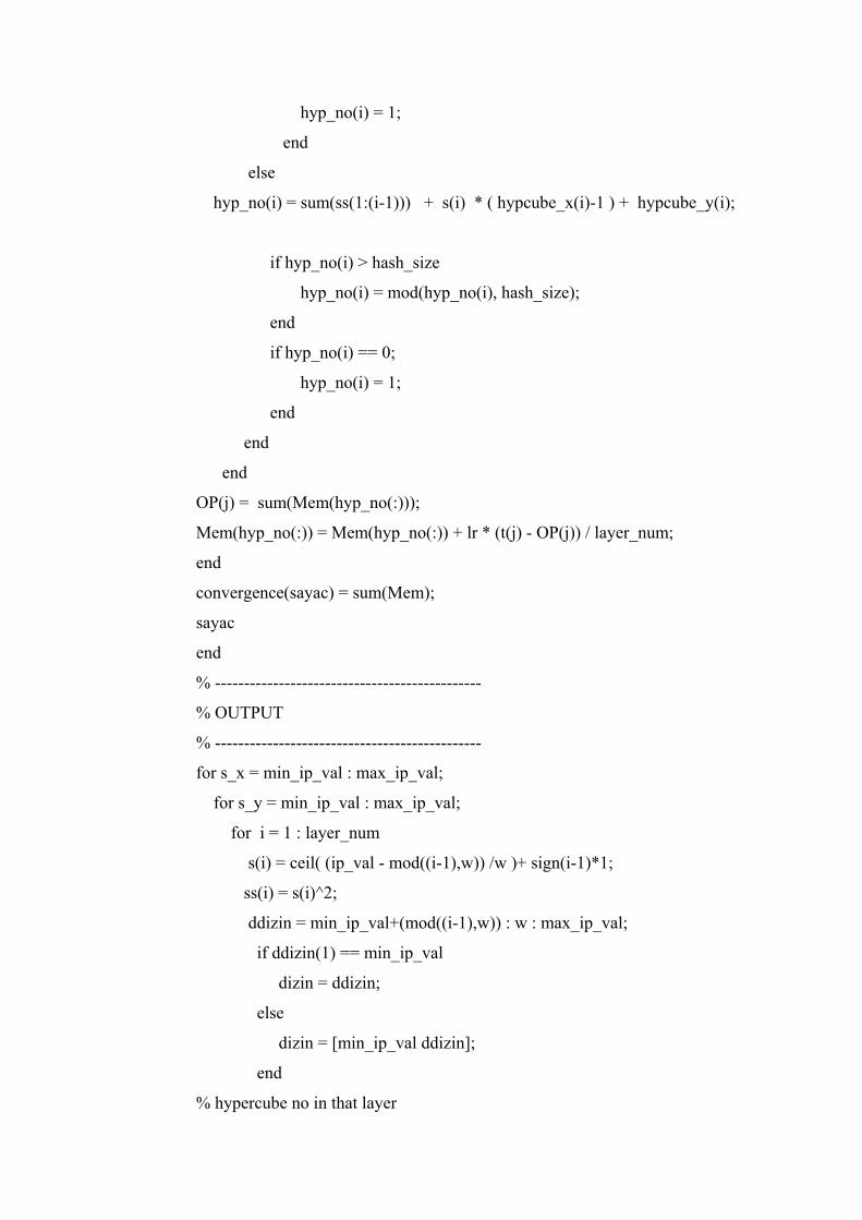
hyp_no(i) = 1;
end
else
hyp_no(i) = sum(ss(1:(i-1))) + s(i) * ( hypcube_x(i)-1 ) + hypcube_y(i);
if hyp_no(i) > hash_size
hyp_no(i) = mod(hyp_no(i), hash_size);
end
if hyp_no(i) == 0;
hyp_no(i) = 1;
end
end
end
OP(j) = sum(Mem(hyp_no(:)));
Mem(hyp_no(:)) = Mem(hyp_no(:)) + lr * (t(j) - OP(j)) / layer_num;
end
convergence(sayac) = sum(Mem);
sayac
end
% ----------------------------------------------
% OUTPUT
% ----------------------------------------------
for s_x = min_ip_val : max_ip_val;
for s_y = min_ip_val : max_ip_val;
for i = 1 : layer_num
s(i) = ceil( (ip_val - mod((i-1),w)) /w )+ sign(i-1)*1;
ss(i) = s(i)^2;
ddizin = min_ip_val+(mod((i-1),w)) : w : max_ip_val;
if ddizin(1) == min_ip_val
dizin = ddizin;
else
dizin = [min_ip_val ddizin];
end
% hypercube no in that layer

hypcube_x(i) = max(find(dizin<=s_x)); % x component
hypcube_y(i) = max(find(dizin<=s_y)); % y component
% hypercube index no
if i == 1;
hyp_no(i) = s(i) * ( hypcube_x(i)-1 ) + hypcube_y(i);
if hyp_no(i) > hash_size
hyp_no(i) = mod(hyp_no(i), hash_size);
end
if hyp_no(i) == 0;
hyp_no(i) = 1;
end
else
hyp_no(i) = sum(ss(1:(i-1))) + s(i) * ( hypcube_x(i)-1 ) + hypcube_y(i);
if hyp_no(i) > hash_size
hyp_no(i) = mod(hyp_no(i), hash_size);
end
if hyp_no(i) == 0;
hyp_no(i) = 1;
end
end
end
%OUTPUT((s_x+abs(min_ip_val)+1), (s_y+abs(min_ip_val)+1)) =
sum(Mem(hyp_no(:)));
OUTPUT(s_x,s_y) = sum(Mem(hyp_no(:)));
end
end
for n = 1 : 181
for m = 1 : 181
z(n,m) = sin(n*pi/180)*cos(m*pi/180);
end
end
D = z - OUTPUT;

% ##############################################
% CONTROL OF 2 DOF MANIPULATOR BY CMAC
% ##############################################
% ----------------------------------------------
% system parameters
% ----------------------------------------------
l1 = 220;
l2 = 220;
r = l1 + l2;
layer = 44;
min_ip = -(l1+l2);
max_ip = (l1+l2);
width = 44; % generalization width
lr = 1; % learning rate
ip = max_ip - min_ip + 1;
tnow = memreq(layer,width,ip);
hash_size = tnow; % hash_size = twn for no hashing
Mem1 = zeros(1,hash_size);
Mem2 = zeros(1,hash_size);
% -------------------------------------------------
% Input & target pairs
% -------------------------------------------------
xt = [-440 -396 -352 -308 -264 -220 -176 -132 -88 -44
0 44 88 132 176 220 264 308 352 396
440 ...
-396 -352 -308 -264 -220 -176 -132 -88 -44 0
44 88 132 176 220 264 308 352 396 ...
-396 -352 -308 -264 -220 -176 -132 -88 -44 0
44 88 132 176 220 264 308 352 396 ...
-396 -352 -308 -264 -220 -176 -132 -88 -44 0
44 88 132 176 220 264 308 352 396 ...
-396 -352 -308 -264 -220 -176 -132 -88 -44 0
44 88 132 176 220 264 308 352 396 ...

-352 -308 -264 -220 -176 -132 -88 -44 0 44
88 132 176 220 264 308 352 ...
-308 -264 -220 -176 -132 -88 -44 0 44 88
132 176 220 264 308 ...
-308 -264 -220 -176 -132 -88 -44 0 44 88
132 176 220 264 308 ...
-220 -176 -132 -88 -44 0 44 88 132 176
220 ...
-176 -132 -88 -44 0 44 88 132 176 ...
440 ];
yt = [ 0 0 0 0 0 0 0 0 0 0 0
0 0 0 0 0 0 0 0 0 0 ...
44 44 44 44 44 44 44 44 44 44
44 44 44 44 44 44 44 44 44 ...
88 88 88 88 88 88 88 88 88 88
88 88 88 88 88 88 88 88 88 ...
132 132 132 132 132 132 132 132 132 132
132 132 132 132 132 132 132 132 132 ...
176 176 176 176 176 176 176 176 176 176
176 176 176 176 176 176 176 176 176 ...
220 220 220 220 220 220 220 220 220 220
220 220 220 220 220 220 220 ...
264 264 264 264 264 264 264 264 264 264
264 264 264 264 264 ...
308 308 308 308 308 308 308 308 308 308
308 308 308 308 308 ...
352 352 352 352 352 352 352 352 352 352
352 ...
396 396 396 396 396 396 396 396 396 ...
0 ];
for i = 1 : length(xt);
if xt(i) == 0 & yt(i) == 0

theta1_d(i) = 0;
theta2_d(i) = 0;
else
theta = ikt(xt(i), yt(i), l1, l2);
theta1_d(i) = theta(1);
theta2_d(i) = theta(2);
end
end
% -------------------------------------------------
% start
% -------------------------------------------------
for k = 1 : 1;
for j = 1 : length(xt)
adres = hypno( layer,width,min_ip,max_ip,hash_size,xt(j),yt(j) );
OP1 = sum(Mem1(adres(:)));
Mem1(adres(:)) = Mem1(adres(:)) + lr * (theta1_d(j) - OP1) / layer;
OP2 = sum(Mem2(adres(:)));
Mem2(adres(:)) = Mem2(adres(:)) + lr * (theta2_d(j) - OP2) / layer;
c(k) = sum(Mem1);
end
end
xd = [-331 -198 -239 -109 201 243 330];

yd = [111 64 285 242 290 149 67];
for i = 1 : length(xd)
adres = hypno( layer,width,min_ip,max_ip,hash_size,xd(i),yd(i));
t1a(i) = sum(Mem1(adres(:)));
t2a(i) = sum(Mem2(adres(:)));
xa(i) = dkx( t1a(i), t2a(i), l1, l2 );
ya(i) = dky( t1a(i), t2a(i), l1, l2 );
err_x(i) = xd(i) - xa(i);
err_y(i) = yd(i) - ya(i);
end
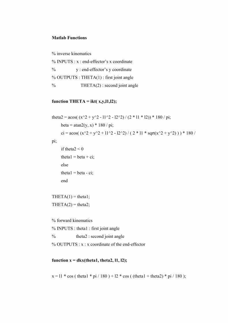
Matlab Functions
% inverse kinematics
% INPUTS : x : end-effector’s x coordinate
% y : end-effector’s y coordinate
% OUTPUTS : THETA(1) : first joint angle
% THETA(2) : second joint angle
function THETA = ikt( x,y,l1,l2);
theta2 = acos( (x^2 + y^2 - l1^2 - l2^2) / (2 * l1 * l2)) * 180 / pi;
beta = atan2(y, x) * 180 / pi;
ci = acos( (x^2 + y^2 + l1^2 - l2^2) / ( 2 * l1 * sqrt(x^2 + y^2) ) ) * 180 /
pi;
if theta2 < 0
theta1 = beta + ci;
else
theta1 = beta - ci;
end
THETA(1) = theta1;
THETA(2) = theta2;
% forward kinematics
% INPUTS : theta1 : first joint angle
% theta2 : second joint angle
% OUTPUTS : x : x coordinate of the end-effector
function x = dkx(theta1, theta2, l1, l2);
x = l1 * cos ( theta1 * pi / 180 ) + l2 * cos ( (theta1 + theta2) * pi / 180 );

% INPUTS : theta1 : first joint angle
% theta2 : second joint angle
% OUTPUTS : y : y coordinate of the end-effector
function y = dky(theta1, theta2, l1, l2);
y = l1 * sin ( theta1 * pi / 180 ) + l2 * sin ( (theta1 + theta2) * pi / 180 );
% hypercube index finder
% INPUTS : layer_num : total number of layers
% w : generalization width
% min_ip_val : minimum input value
% max_ip_val : maximum input value
% hash_size : total number of hashed memory locations
% x_a : x component of the input
% y_a : y component of the input
% OUTPUT : h : hypercubes index no
% OUTPUTS : x : x coordinate of the end-effector
function h = hypno( layer_num, w, min_ip_val, max_ip_val, hash_size, x_a,
y_a)
ip_val = max_ip_val - min_ip_val + 1;
for i = 1 : layer_num
s(i) = ceil( (ip_val - mod((i-1),w)) /w )+ sign(i-1)*1;
ss(i) = s(i)^2;
ddizin = min_ip_val+(mod((i-1),w)) : w : max_ip_val;
if ddizin(1) == min_ip_val
dizin = ddizin;
else
dizin = [min_ip_val ddizin];
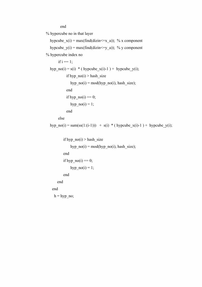
end
% hypercube no in that layer
hypcube_x(i) = max(find(dizin<=x_a)); % x component
hypcube_y(i) = max(find(dizin<=y_a)); % y component
% hypercube index no
if i == 1;
hyp_no(i) = s(i) * ( hypcube_x(i)-1 ) + hypcube_y(i);
if hyp_no(i) > hash_size
hyp_no(i) = mod(hyp_no(i), hash_size);
end
if hyp_no(i) == 0;
hyp_no(i) = 1;
end
else
hyp_no(i) = sum(ss(1:(i-1))) + s(i) * ( hypcube_x(i)-1 ) + hypcube_y(i);
if hyp_no(i) > hash_size
hyp_no(i) = mod(hyp_no(i), hash_size);
end
if hyp_no(i) == 0;
hyp_no(i) = 1;
end
end
end
h = hyp_no;
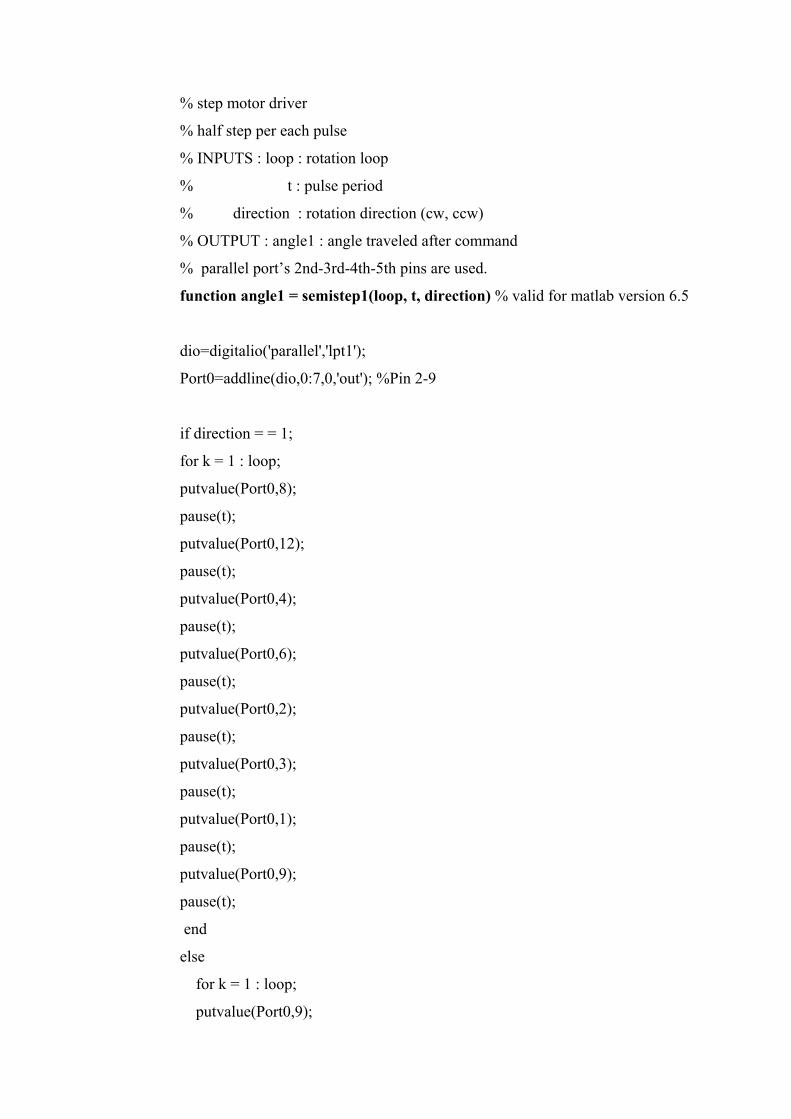
% step motor driver
% half step per each pulse
% INPUTS : loop : rotation loop
% t : pulse period
% direction : rotation direction (cw, ccw)
% OUTPUT : angle1 : angle traveled after command
% parallel port’s 2nd-3rd-4th-5th pins are used.
function angle1 = semistep1(loop, t, direction) % valid for matlab version 6.5
dio=digitalio('parallel','lpt1');
Port0=addline(dio,0:7,0,'out'); %Pin 2-9
if direction = = 1;
for k = 1 : loop;
putvalue(Port0,8);
pause(t);
putvalue(Port0,12);
pause(t);
putvalue(Port0,4);
pause(t);
putvalue(Port0,6);
pause(t);
putvalue(Port0,2);
pause(t);
putvalue(Port0,3);
pause(t);
putvalue(Port0,1);
pause(t);
putvalue(Port0,9);
pause(t);
end
else
for k = 1 : loop;
putvalue(Port0,9);

pause(t);
putvalue(Port0,1);
pause(t);
putvalue(Port0,3);
pause(t);
putvalue(Port0,2);
pause(t);
putvalue(Port0,6);
pause(t);
putvalue(Port0,4);
pause(t);
putvalue(Port0,12);
pause(t);
putvalue(Port0,8);
pause(t);
end
end


