BUREAU OF THE CENSUS STATISTICAL RESEARCH DIVISION REPORT SERIES
SRD Research Report Number: CENSUS/SRD/RR-91/04
CONVERGENCE OF FINITE MULTISTEP PREDICTORS FROM INCORRECT MODELS AND
ITS ROLE IN MODEL SELECTION
bY
David F. Findley Institute of Statistical Science, Academia Sinica
Taipei 11529, Taiwan
and
U.S. Bureau of the Census Statistical Research Division
Washington, DC 20233
This series contains research reports, written by or in cooperation with staff members of the Statistical Research Division, whose content may be of interest to the general statistical research community. The views reflected in these reports are not necessarily those of the Census Bureau nor do they necessarily represent Census Bureau statistical policy or practice. Inquiries may be addressed to the author(s) or the SRD Report Series Coordinator, Statistical Research Division, Bureau of the Census, Washington, D.C. 20233.
Version:12 March 1991
Convergence of Finite Multistep Predictors from
Incorrect Models and Its Role in Model Selection
David F. Findley
Institute of Statistical Science, Academia Sinica
and U.S. Bureau of the Census
Dedicated to Professor Gottfried Klithe in menloriam
Keywords: Time Series Models, Baxter’s Inequality
1. Introduction
In a recent‘ paper [5], we described a generalization to univariate time series mod-
els of the hypothesis testing procedure of Vuong [l2] f or comparing incorrect statistical
models for independent data. The focus of [5] was on model selection criteria related
to one-step-ahead forecasting performance. We suggested there that when p-step-
ahead prediction is the goal, with p > 1, then different test statistics should be used
for each choice of p. To identify appropriate test statistics and determine their asymp-
totic distribution, information is needed about the rate at which predictors based on n
observations converge as n -+ 00. This note provides some of the needed convergence
and distributional results, also for the case of r-dimensional vector time series. Our
approach rests on generalizations of the finite-section inequality and related conver-
1
gence results of Baxter [ 11,121 f or one-step-ahead predictors of scalar time series. To
make our results accessible to a larger circle of readers, we will not formulate them in
the Banach algebra framework utilized by Hirschman [8], but it will be clear to the
mathematical reader that this level of generality is attainable and natural.
2. Baxter’s Inequality (Matrix Form)
For any complex-valued matrix C, let CT denote its transpose and C’ E Cr its
complex conjugate, or Hermitian, transpose. If C* = C, then C is said to be Hermitian
symmetric. Let f(0) d enote a continuous, positive definite Hermitian symmetric, r x r
*matrix function on [-r, z] satisfying f(4) = f(0)‘. It is well known, see [6,p.160] or
[7], that such an f(e) has factorizations of the form
f(e) = A(e (2.1)
and
f(e) = B*(eie)B(eie), (2.2)
where A(z) and B(z) are non-singular-matrix-valued analytic functions on {]z] < l},
A(Z) = 2 aid j=O
B(2) = 2 6jZj
j=O
whose coefficient matrices, aj, bj, have real entrices. We shall impose magnitude restric-
tions on these coefficients with the aid of an increasing sequence of weights v(i) 2 1,
j=O,l,. . ., such that v(j) 5 ~(k)~(]j - Ic]) f or any j,k > 0. This last conditon insures
that the norm defined for matrix functions C(0) = C,“,-, cje’je by means of
2
IlC(@lI = C v(l~l)lcil~
with ]cj] equal to the square root of the largest eigenvalue of cJcj, see [lO,pp.265-6], has
the property that ]]C(e)D(e)]] L ]]C(e)]] ]]D(e)]]. Let C, d enote the set of all continuous
r x r-matrix-valued functions C(0) for which ]/C(e)]] < 00, and let C,+ (respectively
C;) denote the subset whose j-th Fourier coefficient cj is 0 for all j < 0 (respectively,
j > 0). It follows from the preceding norm inequality that f(e) E C, if A(e”) in (2.1)
belongs to C,+ (which implies that A*(e”) E C;). S ince A(z) is nonsingular for all
]z] 5 1, it follows from an argument like that given in [3,p.78] that A-‘(e”) belongs to
Cz if A(e”) does, and then A*(e”)-’ E C;. For us, the important choices of v(j) are
r(j) G 1, v(j) E 2a +ja (cu > 0) and v(j) G p-j (0 < p < 1).
We present now our matrix-function version of the inequality of [2]. Our proof
is an adaptation of Baxter’s, see also [8]. For the reader’s convenience, the complete
proof will be given.
Proposition 2.1. Assume that the factors A(e”) and B(e”) of f(e) in (2.1) and (2.2)
belong to C,+. Then there exist a positive integer no and a constant M, depending only
on these functions, with the following property: if n 2 no, then for any given r x r
matrices gjj 0 5 j < n - 1, the matriz polynominal h(8) = CF!,’ hkeike which satisfies
I
* e -‘j”h(e)f(e)de = gj
--*
for j = 0,‘..,n - 1 will also satisfy the u-norm inequality
where g(0) = Cygigjeije.
(2.3)
Proof: Some additional notation will be helpful. If C E C, is such that C(0) is nonsin-
gular for all 8, we will sometimes use 6 to denote the function C(e)-‘. Also, for any
3
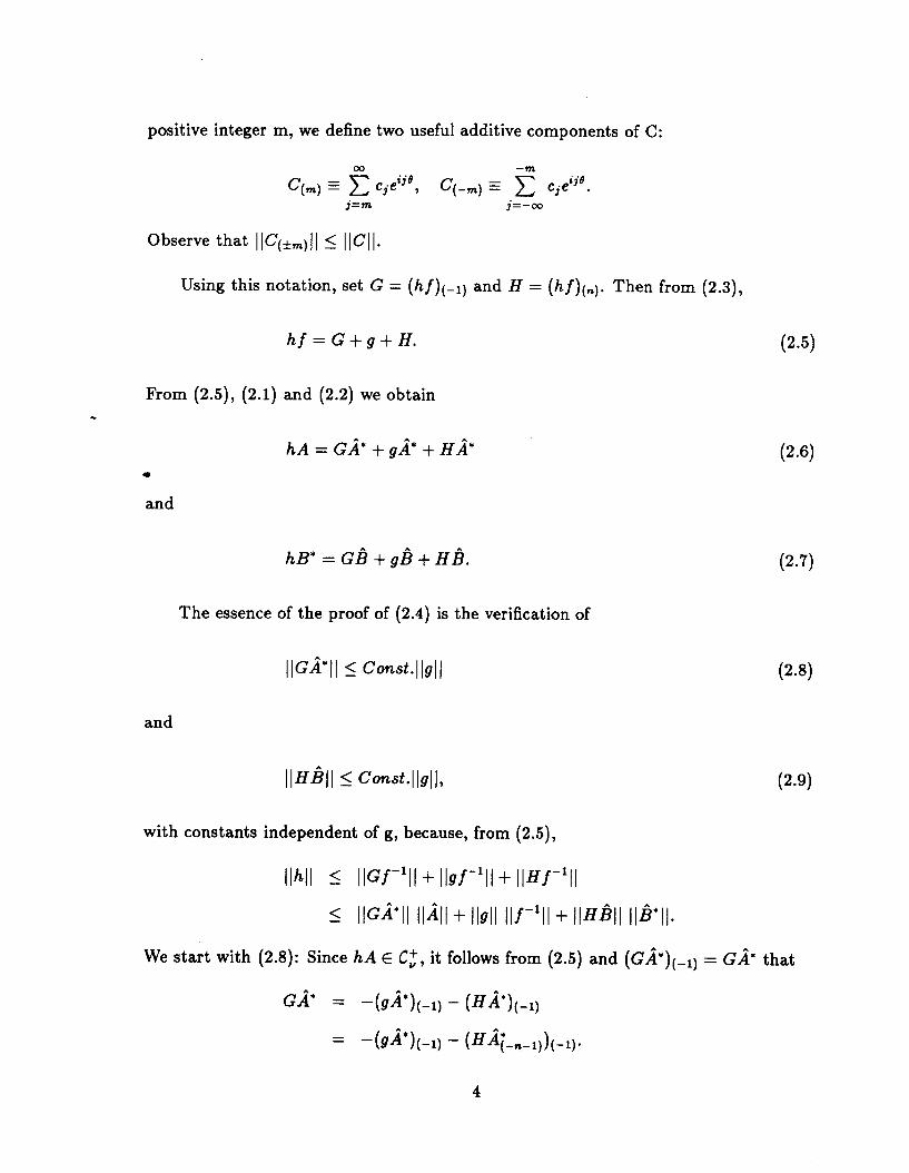
positive integer m, we define two useful additive components of C:
00 --m
C(,) G C Cjeije, C(-,) E C cjeije. j=m j=-00
Observe that IIC~*,)l) 5 IlCll.
Using this notation, set G = (hf)(-1) and H = (hf)(,). Then from (2.3),
hf =G+g+H. (2.5)
From (2.5), (2.1) and (2.2) we obtain
I
and
hA = Gii* + gk + H/i* (2.6)
hB*=G&+gir+H&
The essence of the proof of (2.4) is the verification of
IIG~*ll 5 Const.llsll
and
P-7)
(2.8)
with constants independent of g, because, from (2.5),
llhll 5 llw’ll + lld-‘ll + IIHf-‘ll
5 IIG~‘II INI + ll!Jl IIf-‘II + IIH~II II~“lI.
We start with (2.8): Since hA E C,+, it follows from (2.5) and (GR*)(-,) = GA* that
GA* = -(,a*,,-1, - lHa*)(-I,
= +2*),-q - (Ha;-,-,))(-I).
4
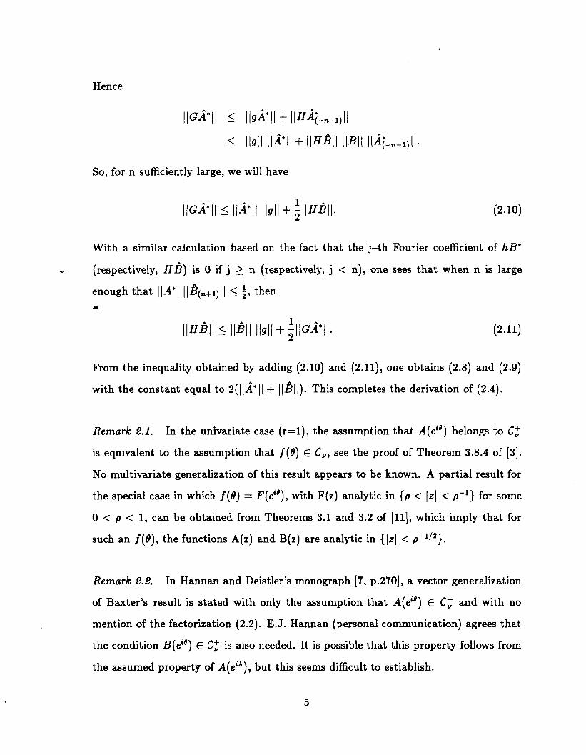
Hence
IIG~*ll 5 llg,*ll + llH&-,111
5 llsll II0 + IIHBII IIBII II+n-I,ll.
So, for n sufficiently large, we will have
IlG~‘ll I lla*ll llsll + ;llHm (2.10)
With a similar calculation based on the fact that the j-th Fourier coefficient of hB* A
w (respectively, HB) is 0 if j > n (respectively, j < n), one sees that when n is large
enough that llA*llll.f3~,,+~~11 I f, then *
IlHfill 5 ll~ll llsll + fllG~*ll. (2.11)
From the inequality obtained by adding (2.10) and (2.11), one obtains (2.8) and (2.9)
with the constant equal to 2(]]a*]] + I]&]]). Th’ is completes the derivation of (2.4).
Remark 2.1. In the univariate case (r=l), the assumption that A(e”) belongs to CL
is equivalent to the assumption that f(e) E C,, see the proof of Theorem 3.8.4 of [3].
No multivariate generalization of this result appears to be known. A partial result for
the special case in which f(0) = F(e”), with F(z) analytic in {p < 1.~1 < p-l} for some
0 < p < 1, can be obtained from Theorems 3.1 and 3.2 of [ll], which imply that for
such an f(e), the functions A(z) and B(z) are analytic in {]z] < p-‘i2}.
Remark 2.2. In Hannan and Deistler’s monograph [7, p.2701, a vector generalization
of Baxter’s result is stated with only the assumption that A(eie) E Cz and with no
mention of the factorization (2.2). E.J. Hannan (personal communication) agrees that
the condition B(e”) E Cz is also needed. It is possible that this property follows from
the assumed property of A(eiX), but this seems difficult to estiablish.
5
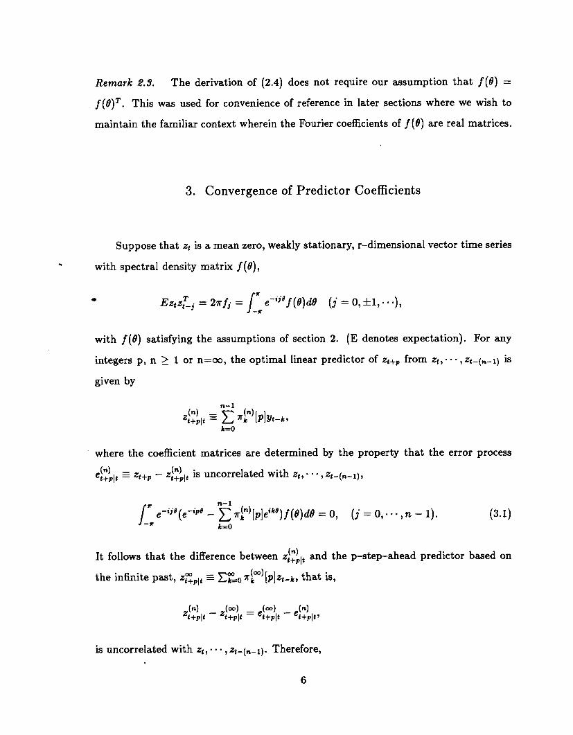
Remark 2.3. The derivation of (2.4) d oes not require our assumption that j(e) =
j(O)‘. This was used for convenience of reference in later sections where we wish to
maintain the familiar context wherein the Fourier coefficients of j(O) are real matrices.
3. Convergence of Predictor Coefficients
Suppose that zt is a mean zero, weakly stationary, r-dimensional vector time series
w with spectral density matrix j(6),
with j(O) satisfying the assumptions of section 2. (E denotes expectation). For any
integers p, n > 1 or n=oo, the optimal linear predictor of zt+P from zt,. . . , zt-(,,-I) is
given by
where the coefficient matrices are determined by the property that the error process
ei:),i, 3 zt+p - ~~~~p .
is uncorrelated with z:, . * a, z+(+i),
/
r n-l
emije(ewipe - C r~)[p]eike) j(6)dlJ = 0, (j = 0,. . . , n - 1). --* k=O
(34
It follows that the difference between .z!$~ and the p-step-ahead predictor based on
the infinite past, ZEplt Z Cgozk ‘“‘lP]zt ok, that is,
(4 z:+plt
(ml _ (=I (4 - Z:+Plt - %+plt - %+plt,
. is uncorrelated with z:, . . . , zt-(,,-11. Therefore,

I_: e+‘<e{ap)[p] - ?rlm)[p]}eiks) j(@&l = fJj P-2) k=O
with
= 2’7r 2 riw'[p] fj-k (3.3)
k=n
for j=O, . . . ,n-1. We are assuming that j(8) and its factors A(e”), B(e”) belong to
C, for some weighting sequence v(j) of the sort considered. Since v(j) 5 v(k)v(k - j)
when 0 < j 5 n - 1 and k 2 n, it is a consequence of (3.3) that
* n-l
c ddI%I 5 (2r 2 y(m)lf-,I) 2 u(k)lriwJ[p]l. j=O m=O k=n
(3.4
The first factor on the right is finite because j E C,. Theorem 7.3 of [13] shows that the
prediction error transfer function e(oo)[p](t3) EZ ebiP8 - CEO riw)[p]eike has the formula
p-1
e(“O)[p](t?) = (C $Jie”j-“‘)$J-l(e), j=O
P-5)
where $(0) = A(e”) f rom which it follows that e(w)[p](t3) E C,. Thus the second
factor on the right in (3.4) is also finite and, applying (2.4), we arrive at the following
generalization of the filter coefficient inequality (11) of [l],
n-l
c W@‘[p] - $‘$I I MO 2 +)l$‘)[p]l < 00. (3.6) k=O k=n
Remark. The inequality given in [l] for the case r=l is for weighted versions of the
coefficients zp’ [l] and TL~’ [l], and is not as convenient for our application as (3.6).
Next, we observe that since 1 < Y(O) 5 v(1) 2 . . ., we have
2 IT!~)[P]I 5 +)-’ 2 v(k)l~~m)[p]l = 0(1/Y(n)). k=n k=n
(3.7)
7
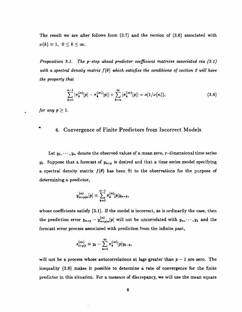
The result we are after follows from (3.7) and the version of (3.6) associated with
v(k) = 1, 0 5 k 5 00.
Proposition 9.1. The p-step ahead predictor coefficient matrices associated via (8.1)
with a spectral density matriz j(9) which satisfies th e conditions of section 2 will have
the property that
n-l
C IdTPl - d~‘bI + 2 ld%l = 0(1/v(n)), k=O k=n
for anypll.
(3.8)
4. Convergence of Finite Predictors from Incorrect Models
Let yr,..., yn denote the observed values of a mean zero, r-dimensional time series
yt. Suppose that a forecast of yn+p is desired and that a time series model specifying
a spectral density matrix j(e) has b een fit to the observations for the purpose of
determining a predictor,
dyn-k,
whose coefficients satisfy (3.1). If the model is incorrect, as is ordinarily the case, then
the prediction error y,+, - y!$Jpln[p] will not be uncorrelated with yn, .. . ,yl and the
forecast error process associated with prediction from the infinite past,
e:;;,, - Y: - 2 “f=)[p]yt-k, k=O
will not be a process whose autocorrelations at lags greater than p - 1 are zero. The
inequality (3.8) makes it possible to determine a rate of convergence for the finite
predictor in this situation. For a measure of discrepancy, we will use the mean square
8
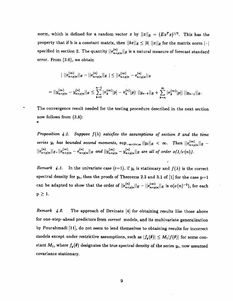
norm, which is defined for a random vector x by ]]x])E = (Exrx)‘j2. This has the
property that if b is a constant matrix, then I ]bx]]z 2 lb] ]]x]]z for the matrix norm I . ]
specified in section 2. The quantity ]Je~~pln]] E is a natural measure of forecast standard
error. From (3.6), we obtain
I Ilef,?$nllE - IIe$!plnIIE I 5 IIe!$,n - e!t?plnlIE
= IIY!$in - YzpInIIE I I$: /rim’ [PI - AP)IPII IIYn-kllE + 2 I~~w’[~]I ([Yn-ilIE* k=n
The convergence result needed for the testing procedure described in the next section
now follows from (3.8): *
Proposition 4.1. Suppose j(X) satisfies the assumptions of section 2 and the time
series yf has bounded second moments, SUP-,<~<~ (]yt(JE < 00. Then IIeL$lnIIE - IIezplnIIEv IIe!$ln - e!$!p[nIIE and IIY!aTL[n - y~~plnll~ are all of order 0(1/v(n)).
Remark 4.1. In the univariate case (r=l), if yt is stationary and j(X) is the correct
spectral density for yt, then the proofs of Theorems 2.3 and 3.1 of [l] for the case p=l
can be adapted to show that the order of ](e!$p,n]]E - ]]I?$$,]]E is o(v(n)-2), for each
P 2 1.
Remark 4.2. The approach of Devinatz [4] f or obtaining results like those above
for one-step-ahead predictors from correct models, and its multivariate generalization
by Pourahmadi [ 111, d o not seem to lend themselves to obtaining results for incorrect
models except under restrictive assumptions, such as ] jy(6)] 5 A&] j(6)] for some con-
stant Ml, where jy(6) designates the true spectral density of the series y:, now assumed
covariance stationary.
9

5. A Prototype Test Statistic for Comparing Models for Prediction
In this section, we assume that yt is a mean zero, stationary vector process whose
m-th order cumulants exist and are absolutely summable, for each m=2,3, ... (As-
sumption 2.6.1 of [3]). Suppose that p-step-ahead forecasts are desired for some p 2 1
and that two competing incorrect models for yt are available, specifying spectral den-
sity matrices j(e) and j(6), both of which satisfy the assumptions of section 2 for the
weighting sequence v(j) z 2’j2 + j1i2. Let e!$,, and $$lt denote the error process of
these models arising from predicting yt+p linearly from yt-j, j > 0. These are stationary
processes satisfying the same cumulant assumptions as yt, and the same is true of the
*difference-of-squared-error process
St+, G e(w)Te(w) -(WIT -(WI t+pp t+plt - ef+,lt et+Plts (5.1)
We define ap = ]]e,($,]]z and Cp E ]]Z~$tJ(z. These quantities measure prediction
performance: if ap < Cp, the model specifying j(X) can be regarded as better for p-
step prediction than the model specifying j(X). W e would like to have a statistical test
for deciding from observed prediction errors whether one of ap or Cp is smaller than the
other.
Let j&(6) denote the spectral density function of the process S,,, - J?S(&+~), ob-
serving that E(Jt+p) = C$ - 5;. Theorem 4.4.1 of [3] shows that N’j2 times the sample
mean from N observations of this process has a limiting normal distribution with mean
0 and variance 2n jb(6). This fact can be expressed as
N
N-‘j2 c S,,,, - N”2(6; - 6;) -+dist. h/(0,2+0)). (5.2) n=l
This result cannot be used directly to obtain a test of the hypothesis op = zip,
because the quantities S,,+, cannot be calculated when only finitely many observa-
10

tions of yt are available. This is where Proposition 4.1 plays a useful role. It en-
ables us to show that N-‘i2 Cf=, S,,+, can be approximated with sufficient accuracy by
Nell2 Cf=, 6n+pln, where
6 n+pln (n)T (4 -(nP 44
SE en+plnen+pln - en+plnen+Pln’
the filters, quantities easily from available
when models ARMA
.
S 5.1. the density f and (6) the
of 2 v(j) 2 ‘I2 and if~up-,<~<~ ll~tll~ < 00, then
&nw N-‘/2E( 5 &+p - $J &+plnl = 0.
n=l n=l (5.3)
Proof : The quantity whose limit is under investigation is bounded above by
N-“2 CL, E1L+p - h+pln I. This latter quantity is bounded above by N-‘/2 times the
sum of
A n F E(etwJT e(O”) (nP’ (4 n+pln n+pln - en+plnen+pln ’ 1 l<n<N -
and the analogous quantities associated with f(6), t o which the argument given below
also applies. Toeplitz’s Lemma [lO,p.250] shows that if
A n = o(nw112) (5.4
holds, then N-‘i2 Cr=, A, + 0. Thus it remains to verify (5.4). By the Cauchy-
Schwarz inequality,
An I I Iei$l,, - eF:pln I IE I le(OQ) n+pln + eZp,n I IE. (5.5)
11
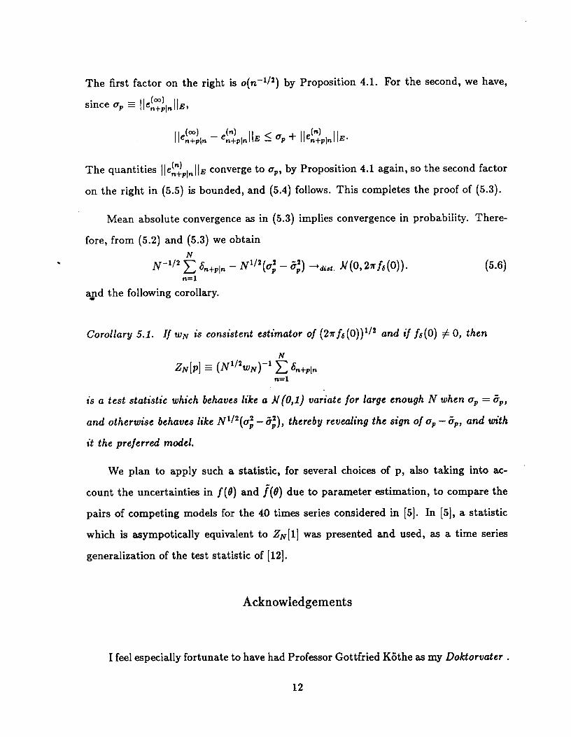
The first factor on the right is o(n -V2 by Proposition 4.1. For the second, we have, )
since up E ]]e~$lnllz,
The quantities
on the right in
IIe~~~ln - e?jplnIIE 5 Op + IIezplnII~*
Ile~plnll E converge to up, by Proposition 4.1 again, so the second factor
(5.5) is bounded, and (5.4) f o 11 ows. This completes the proof of (5.3).
Mean absolute convergence as in (5.3) implies convergence in probability. There-
fore, from (5.2) and (5.3) we obtain
. N-‘12 5 b+pln - N1i2(u; - 5;) -+dist. u(wd6(0)).
n=l
asd the following corollary.
(5.6)
Corollary 5.1. If wN is COnSiSted estimator of (27r j,5(0))1/2 and if j6(0) # 0, then
N
is a test statistic which behaves like a U(O,l) variate for large enough N when ap = cp,
and otherwise behaves like N’f2(ul - Sl), thereby revealing the sign of ap - cp, and with
it the preferred model.
We plan to apply such a statistic, for several choices of p, also taking into ac-
count the uncertainties in j(0) and f”(6) due to parameter estimation, to compare the
pairs of competing models for the 40 times series considered in [5]. In [5], a statistic
which is asympotically equivalent to ZN[l] was presented and used, as a time series
generalization of the test statistic of [12].
Acknowledgements
I feel especially fortunate to have had Professor Gottfried Kiithe as my Doktorvater .
12

While a student, I appreciated his great knowledge, the clarity of his thinking and
writing, and his humor. As a mature researcher, I also admire the ways in which he en-
couraged independent thinking and the high example he set of how to treat colleagues
and students with integrity and warmth.
This article was written while I was the Visiting Research Fellow of the Institute of
Statistical Science of Academia Sinica in Taipei. I am grateful for the excellent research
opportunities provided by this Institute and for the hospitality of the research fellows
and staff there, especially Ching-Zong Wei and Min-Te Chao.
13
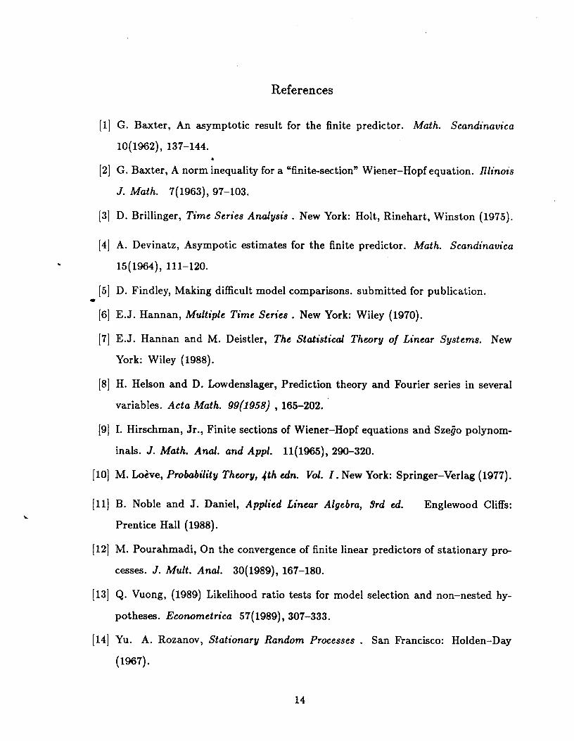
References
[l] G. Baxter, An asymptotic result for the finite predictor. Math. Scandinavica
lO( 1962)) 137-144. .
[2] G. Baxter, A norm inequality for a “finite-section” Wiener-Hopf equation. Illinois
J. Math. 7(1963), 97-103.
(31 D. Brillinger, Time Series Analysis . New York: Holt, Rinehart, Winston (1975).
[4] A. Devinatz, Asympotic estimates for the finite predictor. Math. Scandinavica
15(1964), 111-120.
[5] D. Findley, Making difficult model comparisons. submitted for publication. I
[6] E.J. Hannan, Multiple Time Series . New York: Wiley (1970).
[7] E.J. Hannan and M. Deistler, The Statistical Theory of Linear Systems. New
York: Wiley (1988).
[8] H. Helson and D. Lowdenslager, Prediction theory and Fourier series in several
variables. Acta Math. 99(1958) , 165-202.
[9] I. Hirschman, Jr., Finite sections of Wiener-Hopf equations and Szejio polynom-
inals. J. Math. Anal. and Appl. 11(X%5), 290-320.
[lo] M. Lo&e, Probability Theory, 4th edn. Vol. I. New York: Springer-Verlag (1977).
(11) B. N_ bl o e and J. Daniel, Applied Linear Algebra, 3rd ed.
Prentice Hall (1988).
Englewood Cliffs:
[12] M. Pourahmadi, On th e convergence of finite linear predictors of stationary pro-
cesses. J. Mult. Anal. 30(1989), 167-180.
[13] Q. Vuong, (1989) Likelihood ratio tests for model selection and non-nested hy-
potheses. Econometrica 57( 1989)) 307-333.
[14] Yu. A. Rozanov, Stationary Random Processes . San Francisco: Holden-Day
(1967).
14


