Download - Converging to Convergence - NBER
Converging to Convergence
Michael Kremer
University of Chicago
Jack Willis
Columbia University
Yang You∗
The University of Hong Kong
June 2021
Abstract
Empirical tests in the 1990s found little evidence of poor countries catching up with rich -
unconditional convergence - since the 1960s, and divergence over longer periods. This stylized
fact spurred several developments in growth theory, including AK models, poverty trap mod-
els, and the concept of convergence conditional on determinants of steady-state income. We
revisit these findings, using the subsequent 25 years as an out-of-sample test, and document
a trend towards unconditional convergence since 1990 and convergence since 2000, driven by
both faster catch-up growth and slower growth of the frontier. During the same period, many
of the correlates of growth - human capital, policies, institutions, and culture - also converged
substantially and moved in the direction associated with higher income. Were these changes
related? Using the omitted variable bias formula, we decompose the gap between unconditional
and conditional convergence as the product of two cross-sectional slopes. First, correlate-income
slopes, which remained largely stable since 1990. Second, growth-correlate slopes controlling
for income - the coefficients of growth regressions - which remained stable for fundamentals
of the Solow model (investment rate, population growth, and human capital) but which flat-
tened substantially for other correlates, leading unconditional convergence to converge towards
conditional convergence.
JEL Code: E02, E13, O43, O47
Keywords: Convergence, Institutions, Growth regressions
∗Kremer: Department of Economics, University of Chicago (e-mail: [email protected]) and NBER.Jack Willis: Department of Economics, Columbia University (e-mail: [email protected].) and NBER. YangYou: Department of Finance, The University of Hong Kong (e-mail: [email protected]). William Goffredo FeliceLabasi-Sammartino, Stephen Nyarko, and especially Malavika Mani provided excellent research assistance. We thankthe two discussants, Daron Acemoglu and Rohini Pande, as well as Robert Barro, Brad DeLong, Steven Durlauf,Suresh Naidu, Tommaso Porzio, and seminar audiences at the Portuguese Economics Association, NEUDC, HKUST,the IMF, and Berkeley.
1
1 Introduction
Studies of convergence in the 1990s found no tendency for poor countries to catch up with rich
ones. If anything, there was divergence: rich countries growing faster than poor. National accounts
data showed weak divergence across a large set of countries since the 1960s (Barro 1991), while
historical data, for a smaller set of countries, showed stronger divergence starting as early as the
16th century, with the ratio of per capita incomes between the richest and the poorest countries
increasing by a factor of five from 1870 to 1990 (Pritchett 1997). The lack of convergence was a
major challenge to models where growth is based on accumulation of capital subject to decreasing
returns or where copying technology is easier than developing new technologies. It led to two
responses: first, a rejection of the neoclassical growth models and the development of poverty
trap models and AK endogenous growth models, some of which predict divergence (Romer 1986);
second, an emphasis on underlying determinants of steady-state income, such as human capital,
policies and institutions, leading to growth regressions and tests of convergence conditional on
them (Barro and Sala-i Martin 1992; Durlauf et al. 2005).
To update the stylized facts of convergence, we revisit these empirical exercises with twenty-
five years of additional data. We consider global trends in income and growth, as well as factors
that might determine them – which we term the correlates of growth - such as human capital,
policies, institutions, and culture. We find substantial changes since the late 1980s, in growth, in
its correlates, and in the cross-country relationship between them. While we do not provide a full
analysis of the reasons, or causal determinants, we think this is still useful, as any understanding
of development should match the cross-country patterns.
We begin with absolute convergence – poor countries growing faster than rich, unconditionally
– and document convergence in income per capita in the last two decades. To study the trend in
convergence, we regress ten-year growth in income per capita on income per capita and consider
the evolution of the relationship since 1960. Doing so shows a steady trend towards convergence
since the late 1980s, leading to absolute convergence since 2000, precisely when empirical tests of
convergence fell out of fashion. In terms of magnitude, from 1985-1995 there was divergence in
income per capita at a rate of 0.5% annually, while from 2005-2015 there was convergence at a rate
of 0.7%.1 While lower than the 2% “iron law of [conditional] convergence” (Barro 2012), this still
represents a substantial change. Looking further back to 1960, when the widespread collection of
national income data began, the trend in convergence was initially flat, with neither convergence
nor divergence, followed by a decade of a trend towards divergence in the late 1970s and early
1980s.
Breaking down the trend towards absolute convergence since 1990, by subsets of countries,
provides a fuller picture of the change. There has been both faster catch-up growth and a slow-
down of the frontier. The richest quartile of countries had the fastest growth in the 1980s but
1Our base specification uses income per capita adjusted for Purchasing Power Parity, from the Penn World tablesv10.0, but a similar trend is found using income per capita from the World Development Indicators, measured inconstant 2010 USD, and also when using income per worker.
2
the slowest growth since, being flat in the 1990s and then declining since 2000. In contrast,
the three other quartiles all experienced substantially accelerating growth through the 1990s and
early 2000s, inconsistent with certain poverty trap explanations for the change in convergence, in
which countries catch up once above a certain income threshold. Fewer lower-income countries
have had growth disasters since the mid-1990s – but removing them has little effect on the recent
trend towards convergence; instead, it removes the divergence in the late 1970s and early 1980s.
The trend is also not driven by any one specific region, and convergence becomes stronger upon
removing Sub-Saharan Africa or the bottom quartile of the income distribution from the date set.
Is convergence in the last twenty years just a blip, or does it represent a turning point in world
history? It certainly could be a blip, as other have argued (Johnson and Papageorgiou 2020), for
example due to high commodity prices. Yet, the trend has lasted for 25 years and is robust to
removing resource rich countries, so we entertain the idea that it represents a turning point and
consider its potential causes.
Within the framework of conditional convergence, we classify possible causes into two broad
groups. First, those which lead to faster convergence conditional on growth correlates, which could
include faster spread of technologies due to globalization, as well as greater capital and labor mo-
bility. Second, our main focus, convergence in the growth correlates themselves - human capital,
policies, institutions, culture - which may close the gap between unconditional and conditional
convergence. While recent literature on economic growth and institutions emphasizes the stabil-
ity and persistence of such correlates, using their historical determinants to identify their causal
effects on economic outcomes (Acemoglu et al. 2001; Nunn 2008; Dell 2010; Michalopoulos and
Papaioannou 2013), the finding that certain determinants of growth are highly persistent is not
inconsistent with others changing, potentially rapidly, and being subject to global influences on
policies and culture, for example.
To study whether growth correlates have changed, we classify them into four groups: enhanced
Solow fundamentals – investment rate, population growth rate, and human capital – variables
which are fundamental determinants of steady state income in the enhanced Solow model (Mankiw
et al. 1992); short-run correlates, variables considered by the 1990’s growth literature which may
change in a relatively short time scale, typically policies; long-run correlates, those which change
slowly if at all, and for which we will not have time variation, typically historical determinants
of institutions and geography; and culture. Far from being static, even among highly persistent
correlates we find that many have undergone large changes and themselves converged substantially
across countries, towards those of rich countries.
For the Solow fundamentals and short-run correlates, we examine 35 variables in six categories:
Solow fundamentals, labor force, political institutions, governance quality, fiscal policy, financial
institutions. To tie our hands over which variables we include, we started from a list of variables
commonly used in growth regressions, from the Handbook of Economic Growth chapter on “Growth
econometrics” (Durlauf et al. 2005). We then constrained ourselves to those variables which were
available for at least 50 countries by 1996, and we chose to focus on the period 1985-2015 as a
3
compromise between the number of countries and the number of time periods. Among the 20
variables which are comparable across time, we find significant beta-convergence (a negative slope
of growth regressed on level) in 17. Only credit to the private sector diverged. Moreover, of the
18 variables which were correlated with income in 1985, 15 “improved” on average, meaning they
converged towards those associated with higher income. For a subset of correlates, we are also
able to look further back, and we find similar, albeit slower, trends in 1960-1985.
Using different rounds of the World Value Survey, we also find evidence of convergence in
culture. While culture does show persistence, eight out of the ten cultural variables we consider
have been converging since 1990. For example, views on inequality, political participation, the
importance of family, traditions, and work ethic have all been converging. While limited, the
results of the exercise are consistent with papers in sociology and psychology studying cultural
convergence (Inglehart and Baker 2000 and Santos et al. (2017)). In contrast, convergence was
unlikely or impossible for long-run correlates, and we do not time variation to test for it.
Are these two changes since the late 1980s related: the trend towards convergence in income
and the convergence of many of the correlates of growth? We are naturally unable to do a full
causal analysis and causality can run both ways. On the one hand, an extensive empirical liter-
ature argues that such correlates are important for economic development (Glaeser et al. 2004;
Acemoglu et al. 2005), and the convergence literature itself turned towards convergence conditional
on correlates (determinants of the steady state). On the other hand, modernization theory sug-
gests that causation may run the other way, with converging incomes causing policies, institutions,
and culture to converge. While recent literature uses instrumental variables to provide evidence
on both directions of causation (Acemoglu et al. 2001; Michalopoulos and Papaioannou 2013; Dell
2010; Acemoglu et al. 2019, 2008), these studies build on earlier analysis which focused on stylized
facts from empirical cross-country relationships (Barro 1996; Sala-i Martin 1997; Durlauf et al.
2005; Rodrik 2012), facts which any theory of growth should fit and which we revisit and update.2
To link the trends in growth and its correlates, we develop a simple empirical framework,
revisiting two central cross-country relationships and documenting how they have changed since the
1980s. First, regressing correlates on income; a cross-sectional representation of the modernization
hypothesis. Second, regressing growth on correlates, controlling for income; the basic specification
for both growth regressions and for tests of conditional convergence. By the omitted variable
bias formula, the gap between absolute convergence and conditional convergence is then given by
the product of the slopes of these two relationships (correlate-income slopes and growth-correlate
slopes), allowing us to break down the trend in absolute convergence into trends in these slopes,
together with any trend in conditional convergence. In the main exercise, we do so comparing
1985 to the present, as that is when we have the best data and can run a balanced panel exercise.
In supplementary analysis we also present trends since 1960, which is important as we want to
2Obviously we need to wait another twenty years to perform similar out-of-sample tests of the recent literature.Maseland (2021), in a related paper, studies long-run trends in the relationships between long-run correlates andincome, using the trends to distinguish different models of growth.
4
understand why there was a change in income convergence in the late 1980s.
While the cross-sectional relationships between income and the correlates have changed in
levels, their slopes have mostly remained stable, despite large changes in both income and the
short-run correlates. Among 32 Solow and short-run correlates, regressing the cross-sectional
correlate-GDP slope of 2015 on that of 1985 gives coefficients of 0.90 and 0.89, respectively, and
R-squareds of 0.90 and 0.70. Moreover, while there is substantial prediction error by individual
correlate, on average Solow and short-run correlates themselves have changed as much as would
have been predicted by the changes in income, given the baseline cross-country relationship between
the two.
In contrast, growth regression coefficients have shrunk substantially across the period and
show relatively little autocorrelation. The coefficients of the Solow fundamentals have remained
the most stable, with a slope of 0.86 and an R-squared of 0.95 when regressing coefficients in
2005 on those in 1985. The coefficients of short-run correlates have shrunk the most, such that
there is almost no correlation in coefficients between the periods (slope 0.18, R-squared 0.06). For
example, in 1985, a one standard deviation higher Freedom House Political Rights score predicted
0.6% higher annual GDP growth for the subsequent decade, yet the predictive power is negligible
in the decade 2005-2015. Long-run correlates and culture fall somewhere between the two, with
coefficients which are somewhat stable across the periods, although on average they also shrank.
As a result of the flattening of the growth-correlate relationships, absolute convergence con-
verged towards conditional convergence, by the omitted variable bias formula. This helps to explain
the trend towards absolute convergence, but has conditional convergence itself also become faster?
While conditional convergence regressions typically condition on multiple correlates, our baseline
specification conditions on one variable at a time, because of the difficulty in forming a balanced
panel with multiple correlates and to tie our hand in terms of specification search. In our mul-
tivariate analysis, while not our main focus, we find no obvious trend in conditional convergence
itself, which held throughout the period.
These results suggest an interpretation that is consistent with neoclassical growth models.
Conditional convergence has held throughout the period. Absolute convergence did not hold
initially, but, as human capital, policies, and institutions, have improved in poorer countries, the
difference in institutions across countries has shrunk, and their explanatory power with respect to
growth and convergence has declined. As a result, the world has converged to absolute convergence
because absolute convergence has converged to conditional convergence.
However, this narrative leaves a key question unanswered: why did the growth regression
coefficients shrink? One interpretation, consistent with a Fukiyama end of history view, is that
policies and institutions used to matter, but now that they have converged, they matter less - their
effects are non-linear. For example, perhaps terrible institutions are bad for growth, but so long
as institutions are not disastrous, they matter much less, and there is convergence. However, our
results could also be viewed as demonstrating the limits of our collective understanding: many of
the policies which were significant in growth regressions in the 1990s no longer significantly predict
5
growth today, and basic patterns of divergence which held for centuries have not held for the past
20 years. Consistent with this, perhaps earlier growth-regression specifications suffered from an
overfitting problem and are now failing an out-of-sample test using subsequent data? Relatedly,
it is natural to think that there a very large number of factors determine steady state income,
some observable, many unobservable. The correlation between the observable and unobservable
determinants may have shrunk. While these alternatives would also explain the shrinking of the
gap between absolute and conditional convergence, they cannot explain the trend towards absolute
convergence, although that could result from faster conditional convergence. The multitude of
possible interpretations acts as a reminder of the difficulty of projecting the current trends we
document forward, and the dangers of extrapolating from trends over the past quarter century,
especially considering rising authoritarian populism, climate change, and pandemic threats, a
theme we return to in the conclusion.
This paper describes trends in major macro-economic variables and the relationships between
them, some of which have changed substantially in the last twenty years. The goal is descriptive,
not causal. The first literature we contribute to is that regarding convergence, which flowered
in the 1990s. Despite absolute convergence being a central prediction of foundational growth
models, multiple papers found no evidence for absolute convergence in incomes across countries
(Barro 1991; Pritchett 1997), but evidence of convergence within countries and across countries
conditional on similar institutions (Barro and Sala-i Martin 1992). While we identify off cross-
country variation, Caselli et al. (1996) and Acemoglu and Molina (2021) argue that countries
should have fixed effects in convergence regressions, corresponding to their individual steady-
state incomes. The tradeoffs are discussed at length in Durlauf et al. (2005) and we discuss our
specification choice in Section 2. In short, we think that the country fixed effects absorb exactly
the variation relevant for studying convergence. Consistent with this, if we allow country fixed
effects to vary by decade, then they themselves have converged since the 1990s, so that our results
do still appear in that framework, just absorbed into the “nuisance” parameters. More recently
there have been several important additions to the classic convergence findings. Rodrik (2012)
looks specifically at manufacturing and shows that within manufacturing, there has been absolute
convergence. Grier and Grier (2007), a paper closely related to ours, also considers convergence in
both income and in policies and institutions from 1961-1999. They contrast convergence in policies
and institutions with divergence in incomes, arguing that this difference is hard to reconcile with
neoclassical growth models. We agree with their conclusion for the period 1960-1990, but benefit
from twenty years of additional data, and argue that convergence changed around 1990, and is
since consistent with models of neoclassical growth and inconsistent with a class of endogenous
growth theory models which predict divergence, such as AK models (Romer 1986) or some poverty
trap models.
This is not the only paper to revisit the question of convergence with updated data. Roy
et al. (2016), in particular, make the point that there has been absolute convergence in the last 20
years and, in concurrent work to ours, Patel et al. (2021) emphasize how this is in contrast to the
6
previous stylized facts about convergence. Johnson and Papageorgiou (2020), in contrast, also uses
the latest data and concludes that there is still no absolute convergence. The difference results in
part from Johnson and Papageorgiou (2020) considering convergence from a fixed base date (1960),
while we consider the trend in convergence over a moving time interval, and in part because we are
willing to speculate that the trend in the last twenty-five years represents a fundamental change.
Indeed, while we find a sustained trend towards convergence, we only find actual convergence for a
relatively short period, whilst historically divergence has been the norm for several hundred years
Pritchett (1997).
The paper also adds to the literature on the effects of culture and institutions. Recent papers
use historical variation to identify the effect of institutions and culture on income, using either
instruments (Acemoglu et al. 2001; Algan and Cahuc 2010) or spatial discontinuities (Dell 2010),
and generally find that both play a central role. That empirical strategy requires focusing on long-
run, persistent components of steady-state determinants, which can easily slide into a pessimistic
view: the things that matter for growth can only change very slowly. However, while some, such
as legal systems and trust, have deep historical roots and may change very slowly (Michalopoulos
and Papaioannou 2013), many change rapidly, and there is no contradiction in culture both having
a long-run effect and being subject to recent change. For example, gender roles have deep and
important historical determinants (Alesina et al. 2013), but they have also changed substantially in
the last 50 years, differentially across countries. While historical determinants continue to persist,
we should also remain open to asking how recent changes in policies and institutions have affected
growth, especially when considering policy changes.
Our growth regressions exercise also provides an out-of-sample test of sorts for the predictive
power of policies and institutions: with a limited sample size and many potential covariates, the
growth regressions literature is vulnerable to overfitting; events since the publication of earlier
papers provides a (limited) out-of-sample dataset (Hastie et al. 2009).
Finally, in studying changes to, and convergence in, policies, institutions, and culture, the paper
adds to expansive literatures in political science, sociology, and psychology whereby the diffusion
and convergence of numerous policies, institutions and cultural traits have been documented and
studied (Dobbin et al. 2007).3 Some of the changes in correlates have been gradual, possibly
consistent with modernization theory (Acemoglu et al. 2008; Inglehart and Baker 2000), and
indeed we do find that on average changes in correlates are consistent with predictions from income
growth, based upon the cross-country relationship. However, many recent changes in policies and
institutions are dramatic, such as global trends in the adoption of VATs, or marriage equality, or the
Me Too movement, which may be better thought of as technology adoption through information
diffusion. This technology diffusion may be passive or may, for example, result from the work
of international organizations, who provide norms and information on perceived best practices
(Clemens and Kremer 2016), and sometimes directly incentivize the adoption of different policies
3The social science literature on the diffusion of policies has proposed four theories for policy diffusion: socialconstruction, coercion, competition, or learning. See Dobbin et al. (2007) for a review.
7
through conditionality. For example, the “Washington Consensus” encouraged lowers tariffs, lower
inflation, and (word) of state-owned firms, all of which have been broadly adopted since. The end
of the cold war ushered in a period of growth in democracy. In a closely related paper, Easterly
(2019) argues that such “Washington Consensus” reforms may have been better for growth than
previously believed, as growth has been higher recently in countries which adopted them. Finally,
convergence and diffusion of culture are central topics in sociology and psychology. Two recent
examples studying them using the World Value Surveys (among other data sources) as we do, are
Inglehart and Baker (2000) and Santos et al. (2017).
The paper proceeds as follows. In section 2, we present the results on absolute convergence
in income per capita and document a trend towards convergence since the 1990s. In section 3,
we consider global trends in the correlates of growth - policies, institutions, human capital, and
culture - and document considerable convergence across multiple dimensions. In section 4, we
relate the trend towards convergence in income to the convergence in the correlates of growth, first
considering the cross-country relationships between income and correlates (modernization theory),
which have remained stable, then turning to the cross-country relationships between correlates
and growth (growth regressions), which have flattened, and finally turning to the gap between
unconditional and conditional convergence, which has shrunk. Section 5 concludes.
2 Convergence in income
Neoclassical growth models predict convergence towards steady-state income: poor countries
should catch up with rich countries, at least among countries with similar underlying determinants
of steady-state income. Empirical tests in the 1990s of absolute convergence - convergence across
countries without conditioning on determinants of steady state income - found little evidence for
it: if anything, rich countries were growing faster than poor (Barro 1991). We begin by revisiting
these tests of absolute convergence, with 25 additional years of data. We use the same data sources
and focus mainly on β-convergence, defined below.4
2.1 Empirical setup: measuring convergence
The convergence literature in the 1990s used three different datasets. First, standard cross-
country sources such as the World Development Indicators and the Penn World Tables, which
covered a sizeable span of countries from the 1960s onwards. Second, the Maddison dataset, which
collected many sources of data to derive income per capita going back much further in time, for a
smaller set of countries, which showed that divergence had been the norm for several hundred years
(Pritchett 1997. Third, within-country panel datasets, to look at convergence within countries.
For example, Barro and Sala-i Martin (1992) examined convergence within the US.
4Parallel results for σ-convergence are in Figure 1 Panel (b) and Appendix Figure A.5 Panel (b) with a fixedcountry sample
8
Our goal is to document what has happened to global cross-country convergence since the
heyday of the literature in the 1990s. As such, we use the standard cross-country data sources,
which cover 1960-present. In the main specification, we use the GDP per capita, adjusted for
Purchasing Power Parity (PPP) from the Penn World Tables v10.0.5 It is an unbalanced panel,
as for many countries GDP per capita data only becomes available part way through the period.
Nevertheless, we use the unbalanced panel for our main specification so as not to drop many of
the poorer countries which become available later in the period (we also show robustness to using
balanced panels, which make little difference to our results). We also drop very small countries and
those which are extremely reliant on natural resource rents, as is common in studies of convergence.
Specifically, we drop countries whose maximum population during the period was < 200, 000, and
those for whom natural resources accounted for at least 75% of GDP (as reported in the World
Development Indicators) at some time during the period. 6
We examine both β-convergence and σ-convergence. β-convergence is when poor countries
grow faster on average than rich, while σ-convergence is when the cross-sectional variance of (log)
income per capita is falling over time. The relationship between the two notions of convergence is
well documented (Barro and Sala-i Martin 1992; Young et al. 2008). We focus on β-convergence
for most of the analysis, with equivalent results for σ-convergence reported in the Appendix.
β-convergence β-convergence is when poorer countries grow faster on average than richer coun-
tries. Specifically, at a given time period t, it is when the country-level regression
log(GDPi,t+∆t)− log(GDPi,t) = α+ βlog(GDPi,t) + εi,t
has a negative β coefficient, where log(GDPi,t) is Log GDP of country i at time t. To show how β-
convergence has changed over time, we plot βt vs. t, where βt comes for the following country-year
level regression, clustered at the country level (µt is a year fixed effect on growth):
log(GDPpci,t+∆t)− log(GDPpci,t) = βtlog(GDPpci,t) + µt + εi,t (1)
Much of the existing empirical convergence literature plots how β varies when holding the
starting point t fixed (often at 1960) and varying the end point, t+ ∆t. Since we are interested in
how the process of convergence may itself have changed over time, we instead hold ∆t fixed and
vary t. In the main specification we use 10-year averages, i.e. ∆t = 10.7
5Specifically, for growth rates we use the variable “rdgpna”, real GDP at constant 2017 national prices (2017USD), and for growth levels we use “rdgpo”, output-side real GDP at chained PPPs (2017 USD), as recommendedby the PWT user guide.
6Figure A.1 shows the β-convergence after excluding small population countries and major mineral exporters.7The dependent variable is the annualized growth — the geometric average growth rate in the next decade.
9
2.2 Results: converging to convergence
Figure 1 shows the scatter plot and regression of equation 1 for each decade since 1960. Con-
vergence corresponds to a negative slope, and the shift to convergence since 2000 can clearly be
seen in the raw data. Figure A.2 presents summary boxplots of these basic scatter plots, plotting
the average growth by income quintile for each decade.
Figures 2a and 2b show the β- and σ-convergence coefficients from these regressions over the
whole period 1960-2007. The first striking result is that there has been absolute convergence since
the late 1990s, precisely when the best-known empirical tests of convergence were published. The
point estimate for β-convergence becomes negative in the early 1990s, becoming significant in the
late 1990s and staying significant since. Table 1 shows a point estimate of -0.65 in the 2000s, and -
0.76 in the ten years after 2007, the most recent period we can consider. σ-convergence, represented
by a negative slope in Figure 2, started slightly later, with the standard deviation in GDP per
capita falling since the early 2000s. The difference in timing is consistent with β-convergence being
a function of subsequent 10-year average growth.
The second result is that there has been a trend towards β-convergence - converging to conver-
gence – since 1990. The coefficient started at around 0.5 in 1990 and has trended down towards
-1 today. Looking further back to 1960, initially there is no clear trend, and then there is a
trend towards divergence in the 1980s.8 Table 1, Column (2), reports the results of our basic
absolute convergence regression, Equation 1, with the addition of a linear year variable interacted
with log(GDPi,t). The interaction terms, representing the “convergence towards convergence”, is
negative and significant, with a point estimate of -0.025. The trend towards convergence is also
apparent in the σ-convergence figure, where it is represented by a gradual decrease in slope, i.e.
concavity of the plot.
This trend towards convergence is consistent with models of growth in which capital is subject
to diminishing marginal returns, or where catch-up growth is easier than growth at the frontier.
It is inconsistent with models of growth which predict long-run divergence, such as AK models, or
some poverty trap models.
2.3 Econometric considerations and robustness to alternative specifications
There is an extensive literature on the tradeoffs of different econometric specifications to test
for convergence, summarized in Durlauf et al. (2005). We follow the most standard approach,
testing for β convergence using OLS with fixed effects for year, clustered at the country level. This
approach is not without limitations, which we discuss below, but it is transparent and captures
the cross-country variation which is our main focus.
We begin by replying to the three main critiques of the specification noted in the comment
of Acemoglu and Molina (2021): unobserved country fixed effects, cross-country heterogeneity in
8In subsequent robustness exercises, not using PPP adjustments, the trend looks more like a steady trend towardsconvergence since 1960, except for a major reversal in the 1980s
10
convergence rates, and using 10-year growth rather than annual growth. We then discuss several
additional considerations and robustness questions, such as whether measurement error may drive
towards convergence through mean reversion, whether results are driven by panel imbalance, in
particular the larger number of poor countries entering the panel over time, and whether results
depend on the macroeconomic dataset used.
Specification, country fixed effects, and heterogeneity Our regression specification as-
sumes homogeneous rates of convergence across countries and does not account for potential dif-
ferences in steady state income, as discussed in Acemoglu and Molina (2021). We agree with the
empirical finding of the authors and Caselli et al. (1996): the coefficients on current income change
substantially when incorporating heterogeneity and country fixed effects, with strong convergence
towards countries individual steady state income levels throughout, at a rate of at least 10%.
However, we disagree that their specification is more economically meaningful for the question of
convergence (or, in particular, that the coefficient on income in these specifications can be inter-
preted as causal). It is a different exercise, and one which is not without its own econometric issues
(Durlauf et al. 2005).
We are interested in what has been happening across countries, over time; by definition, country
fixed effects absorb cross-country differences and treat them as nuisance parameters. We agree
that there are likely to be cross-country differences in steady-state income, but we wish to know
how these differences have evolved. A priori, we do not know whether convergence to a fixed
steady state, or evolution of country-level ”steady state” income itself, is likely to be a more
important determinant of growth, so we do not want to assume away the latter. Investigating
the evolution of the country-level steady state is precisely our exercise below, when we turn to
conditional convergence, and to whether the potential determinants of steady-state income have
converged. We view doing so with variation which we can explain – changes in correlates – as
providing additional insights, but we can also do so with a fixed effects approach, which can be
interpreted as another form of conditional convergence. To do so, however, we need to allow for
the possibility that country ”fixed effects” vary over time. Specifically, we modify the framework
of Acemoglu and Molina (2021) to allow country fixed effects to vary by decade:
log(GDPi,t+∆t)− log(GDPi,t) = βdlog(GDPi,t) + µt + γi,d + εi,t (2)
γi, d being a country-decade fixed effect.
Table A.1 reports the βd estimated with average decade growth in Panel A and annual growth
in Panel B, confirming the results of Acemoglu and Molina (2021). The coefficient stays strongly
negative since 1960. The magnitude is quite stable and does not exhibit any declining pattern over
time. We also find that using annual growth gives stronger convergence and we speculate below
that annual GDP measurement errors might bias upwards a short-term reversal pattern.
In this paragraph in an earlier version of this paper, in analysis undertaken to respond to
Acemoglu and Molina’s discussion at the NBER Annual Conference on Macroeconomics, we in-
11
correctly claimed that the fixed effects in this model show little stability over time. Our error
was pointed out in Acemoglu and Molina (2021), their subsequent discussion paper. We thank
the authors for this correction and have updated this paragraph accordingly (and removed the
appendix figure which it referred to). As shown in Acemoglu and Molina (2021) the country fixed
effects in this model are stable over time and have a high F-test statistic. This persistence of the
fixed effects is primarily from the persistence of country income levels; country growth rates show
little autocorrelation from decade to decade.
In this specification, country-decade fixed effects have converged across countries since 1990s,
suggesting that much of the action for studying the global income distribution may be being
absorbed by these fixed effects. Figure A.3 plots standard deviations of fixed effects over time
with a rolling time window of ten years. We see a fall in the standard deviation of the country
fixed effects since 1990, the period in which we see a trend towards unconditional convergence in
our preferred specification. This encourages us to study whether unconditional convergence has
converged towards conditional convergence, the question we turn to below.
Moreover, the country fixed effects approach has its own econometric limitations, discussed
further in Durlauf et al. (2005). The convergence coefficient in the country fixed effects model, βd
in Equation 2, is identified from time-series variation for all years in decade d, while the convergence
coefficient in our main specification, βt in Equation 1, is identified from cross-sectional variation
in year t. Bernard and Durlauf 1996 shows that the two specifications may give very different
answers and argues that the time-series βd is a good estimate of convergence only if the sample
distribution is a good approximation of the true underlying growth process; if historical growth is
not stable, then the time-series model can be substantially biased. Our analysis includes uses a
large set of countries, most of which experienced substantial changes in growth correlates during
the period, potentially perturbing them far away from their steady states.
Averaging period Many of the original convergence studies used a fixed baseline year, consid-
ering how convergence in income per capita changed when varying the endline year. We argue
that to consider trends in convergence itself, rather than use a fixed baseline year, it is better to
consider convergence over a fixed interval of time, and how it changes when varying the baseline
year. This raises a natural question of what the fixed interval of time should be and whether
that interval matters. In the main results, we used a 10-year interval, considering 10 years a good
trade-off between allowing us to see medium-frequency trends, without overloading the trend with
annual noise. Acemoglu and Molina (2021) suggest we should use annual data. We think that
annual data gets at high frequency phenomenon (e.g. weather streaks, business cycles), while ten
year data gets at lower frequency phenomenon, such as long-run growth. Annual data is likely to
introduce substantial noise. If this noise is measurement error in GDP, then growth regressions
will be biased towards convergence and this bias will be larger over shorter periods, via mean re-
version. Figure A.4 shows how the convergence coefficient varies when using 1-, 2-, 5- and 10-year
averages. 10-year averages show the clearest trend towards convergence. Once we get to 1-year
12
averages, the year-to-year variation dominates, and the trend which is apparent in 5- and 10- year
averages is much less apparent.
Balanced panel Since the number of countries in the dataset is growing over time, our results
could reflect the inclusion of the new countries over time, rather than global trends. To investigate
this, we show, by decade, what convergence looks like from that decade until present day, among
the balanced panel of countries whose data is available from the start of that decade. So, for
example, for the 1970s, we plot the 10-year average convergence coefficient, from 1970 to present,
for the set of countries who are in the dataset since 1970.
Figure A.5 displays the results of these investigations which hold the set of countries fixed over
time. It shows that the change in convergence has little to do with the expansion of the set of
countries over the time period - results are remarkably robust to different balanced panels, showing
that the original results do indeed reflect a trend towards convergence since 1990.
While the trend towards convergence began around the time of the dissolution of the Soviet
Union, the repercussions of which may have been an important driver of the change in convergence,
the robustness of the trend to countries which existed before 1990 shows that the change was not
mechanical from the addition of the former Soviet countries.
Measure of income Figure A.6 shows that our finding of a trend towards convergence is not
specific to looking at income per capita (as opposed to per worker), nor to using income per capita
in Purchasing Power Parity (PPP) adjusted terms from the Penn World Tables v10.0. Namely, we
find a broadly similar pattern using income per worker instead of income per capita, using different
measures of income from the PWT, and using the World Development Indicators data with income
measured in constant 2010 US dollars. Indeed, in the later, the trend is more apparent, and seems
to start from 1960, again with a decade of regression in the 1980s.
2.4 Which countries have driven the change?
To provide more details on the trend to absolute convergence, and to take a first step towards
understanding its causes, we consider which countries have driven the change. We do so mainly
by showing how the trend in convergence changes when removing different groups of countries.
Faster catch-up growth and a slow-down of the frontier Two very different and popular
narratives could each lead to the observed trend to convergence: stagnation of the frontier – a
drop in the growth rate of richer countries; or faster catch-up growth – a rise in the growth rate
of poorer countries.
Figure 3 shows average 10-year growth rate by income quartile, where income quartile is re-
calculated each year. The richest quartile of countries had the highest growth rate of all quartiles
in the 1980s and then switched position entirely to have the lowest growth rate since 2000. The
shift was driven both by a slow-down of growth at the frontier - the richest quartile of countries
experienced flat growth in the 1990s and then a growth slowdown since 2000 – and faster catch-up
13
growth - the other three quartiles experienced a substantial acceleration in growth in the 1990s.
Removing one quartile at a time from our standard test for convergence, Figure A.7, it does appear
that in the last decade the trend towards convergence is driven by the richest quartile versus the
other quartiles, and that the poorest quartile has if anything been a drag on the trend towards
convergence within the other quartiles.
Fewer growth disasters and more growth miracles Figure A.8 presents the trend in coef-
ficients from Equation 1 when excluding countries which experienced disasters or growth miracles.
The trend towards convergence remains robust, whether we drop episodes of especially low or
episodes of especially high growth. Interestingly, the reversion in the 1980s disappears when ex-
cluding countries which had a negative 10-year growth rate.
Which regions are driving the change? Figure A.9 presents the trend in coefficients from
Equation 1 when excluding countries from different regions. Again the trend remains robust,
although the trend towards convergence in the last twenty years becomes stronger upon excluding
Sub-Saharan Africa.
2.5 Club convergence
Convergence has been documented among OECD countries (or rich countries) as a group of
relatively homogeneous countries (Barro and Sala-i Martin 1992), as evidence for club convergence
– convergence among groups of countries which have similar institutions and culture. We revisit
this result and show convergence among the rich countries has slowed and shifted towards the
general global convergence pattern.
Figure A.10 plots the convergence coefficients in the country sub-sample with income above
the Xth percentile.9 Three decades from 1965 to 1995 yield a similar pattern - strong convergence
among high-income countries (above the 60 percentile) while overall there was little absolute
convergence. This pattern has changed in the period from 1995 to 2005, and in the most recent
decade, convergence holds across a sample containing all countries, while convergence among the
top 40% of countries by income has stopped.
These results, together with the above finding that growth has increased across the bottom three
quartiles, are inconsistent with certain poverty trap explanations for the trend towards absolute
income convergence. Namely, we see no evidence of there being an income threshold above which
there is convergence, with more countries crossing the threshold over time.
3 Convergence in correlates of income and growth
We next consider global trends in factors that might be determinants of growth - policies,
institutions, human capital, and culture - using the same empirical approach as above. While
9X = 0 corresponds to absolute convergence. X stops by 80, corresponding to the top 20% high-income countries.The sample size would be too small to obtain stable β if X rises above 80.
14
much recent literature emphasizes the persistence of institutions over time (Acemoglu et al. 2001;
Michalopoulos and Papaioannou 2013; Dell 2010), we find substantial change and convergence.
Overall, 17 out of the 32 Solow fundamentals and short-run correlates for which we have temporal
variation exhibit β-convergence from 1985 to 2015, and the correlates have generally converged in
the direction of those of more advanced economies, towards what we term development-favored
institutions. Moreover, culture has also convergence, with 8 out of 10 measures of culture we
consider displaying β-convergence in the World Value Surveys data.
3.1 Policies, institutions, measures of human capital, and cultural traits con-
sidered
We divide such potential correlates of income and growth into four groups: enhanced Solow
fundamentals – investment rate, population growth rate, and human capital – variables which are
fundamental determinants of steady state income in the enhanced Solow model (Mankiw et al.
1992); short-run correlates, other policy and institution variables considered by the 1990’s growth
literature which may vary at relatively high frequency; long-run correlates, institutions and their
historical determinants which do not change or which only change slowly, which have been the
focus of the recent institutions literature, and geographic correlates of growth; and culture.
To tie our hands, we started from a list of variables commonly used in growth regressions,
from the Handbook of Economic Growth chapter on “Growth econometrics” (Durlauf et al. 2005),
constraining ourselves to those variables which covered at least 40 countries from 1996. We then
added to this list numerous cultural variables and historical determinants of institutions which
have played a central role in the empirical growth literature since Durlauf et al. (2005). While we
obviously cannot consider convergence for historical or geographic variables – they are however
included in the empirical exercises in the next section – we are able to study convergence of mul-
tiple cultural variables, albeit with a smaller country sample than for the policy and institutional
variables.
Table 2 summarizes the data sources and sample period of the resulting correlates. There are 5
enhanced Solow fundamentals and 27 short-run correlates divided into four broad categories: po-
litical institutions, governance, fiscal policy, financial institutions. Not all the short-term correlates
are comparable over time, for example the World Governance Indicators and Heritage Freedom
Scores are standardized each year. We obviously cannot study convergence nor average changes
for such variables, but we include them in the table as we do use them for our analysis of the
gap between unconditional and conditional convergence, in Section 4 of the paper. For certain
figures in the paper, we pick one representative variable from each category, displayed in bold in
the table: Polity 2 score, the WGI rule of law, government spending (% GDP), credit provided
by the financial sector (% GDP). Equivalent figures with the other variables can be found in the
Appendix.
To help interpret the direction of change of correlates, Table 3 Column (3) shows which cor-
15
relates were ”development-favored” in 1985 (or the earliest available year), defined by their cor-
relation with log GDP in 1985. Correlates are defined as high (or low) development-favored if
the coefficient from regressing the correlate on log GDP is positive (or negative), with statistical
significance at a 10% level. A high-income country tends to have a higher Polity 2 score, higher
rule of law score, higher government spending (as a % of GDP), more financial credit, and higher
education attainment. Five correlates cannot be signed: taxes on goods and services, tax burden
score, military expenditure, inflation, and central bank independence.
We first supplement Solow fundamentals with two measures about the labor force: gender
inequality in education (male minus female in educational attainment) and labor force participa-
tion rate. High-income countries enjoy more gender equality in education and lower labor force
participation.
Then, we use five variables to measure political institutions: the Polity 2 score from the Center
of Systematic Peace (1960-2018), the Freedom House political rights score (1973-2018), the Free-
dom House civil liberty score (1973-2015), the Press Freedom score (1979-2018),10 and the political
stability score (1996-2018) from Worldwide Governance Indicators (WGI).
Governance variables - distinct from political institutions - measure whether the public system
functions well. We use four variables (1996-2018) from the WGI Project: government effectiveness,
regulatory quality, the rule of law, control of corruption; and five variables (1995-2019) from
the Index of Economic Freedom by the Heritage Foundation: Overall economic freedom index,
government integrity, business freedom, investment freedom, and property rights. The sample size
of countries in the Economic Freedom database rises from 97 in 1995 to 145 in 2005, and then
159 in 2015. Variables under the governance and political institutions categories are all positively
correlated with economic development.
The fiscal policy category mainly captures the following three dimensions: taxation, tariffs, and
government interventions / expenditures. Taxation measurements include taxes on income and
capital gains (percentage of total tax revenue), taxes on goods and services (percentage of total tax
revenue), and a tax burden score. Equal-weighted and value-weighted tariffs are measures of the
policy-induced barriers to trade. A state with strong government interventions and expenditures
tends to have a lower private investment (% total investment), more government spending (%
spending), and higher military expenditure. In general, high-income countries are more likely to
adopt free trade and low government intervention, but there is not clear pattern in our data on
taxation.
The financial institutions category includes six variables: a central bank independence index
constructed by Garriga 2016; inflation, credit to the private sector (% GDP), and credit provided
by the financial sector (% GDP), all from the WDI; and financial freedom and investment freedom
scores from the Index of Economic Freedom. Higher financial development is positively associated
with economic development, while central bank independence (CBI) and inflation are ambiguous
10The press freedom score ranges from 0 to 100. A high score represents less press freedom in the original data.We transform the data as 100 minus the original data so that high score translates into more press freedom
16
according to our approach. The high inflation of 1990 was not constrained to developing countries,
but a global issue. Central bank independence adoption rose over time and inflation was brought
under control (Rogoff 1985; Alesina and Gatti 1995; Fischer 1995; Alesina and Summers 1993;
Grilli et al. 1991; Alesina 1988).
The following sections examine average changes in correlates from 1985 to 2015 as well as their
rate of convergence, βInst, estimated from the following equation:11
∆1985−→2015Insti = βInstInsti,1985 + α+ εi
The country sample is time-varying (mostly increasing) as datasets add new countries into the
sample. In the Appendix, we also plot the standard deviations of the correlate metrics as the
σ-convergence for correlates (Figures A.11 - A.13).
Before presenting results for individual correlates, we test the convergence of all of our short-
run correlates jointly in table A.2, which presents the joint significance of each category using
seemingly unrelated regressions. All variables are available since 1996. Thus we report results for
1996-2006 in Panel A and 2006-2016 in Panel B. For both decades, we confidently the hypothesis
that convergence in correlates does not exist.
3.2 Enhanced Solow fundamentals
Human capital Human capital is a robust predictor of income growth, as emphasized in the
seminal literature Lucas Jr (1988), Barro (1991), Mankiw et al. (1992), Sala-I-Martin (1997), Barro
and Lee (1994).12 Education augments labor productivity (Lucas Jr (1988)), facilitates techno-
logical progress (Romer (1990)), and can help promote structural transformation into industry
(Squicciarini and Voigtlander (2015)).13
We measure time-varying human capital with the Barro-Lee average schooling years of popula-
tion, age 20-60. Figure A.14 Panel C reports the β-convergence. The convergence in human capital
starts from 1975. Since 1975, poor countries start to gain faster growth in educational attainment
and gradually catch up with rich countries. In addition, education levels in some well-educated
populations have stagnated, and the data implies that 13 average years of education appears to be
a soft cap for many countries.14 We also observe a meaningful shrinking in education attainment
inequality across gender. The education gender gap reduced by 8.1% per decade on average.
11If data were not available in 1985, we use the earliest available year for the analysis. For example, the rule of lawscore from WGI start in 1996. Table 3 Column (4) reports the 1996 average and the baseline year for the correlateconvergence βInst in Column (7) is 1996 as well.
12While human capital is not something which can be directly manipulated by policy, many policies can signif-icantly influence educational attainment, such as budgetary decisions, school-building campaigns, curriculum, andminimum school leaving age.
13See Krueger and Lindahl (2001) for extensive reviews on micro and macro empirical evidence on schooling andgrowth.
14In 2010, only nine countries - Switzerland, Denmark, United Kingdom, Iceland, Japan, South Korea, Poland,Singapore, United States - have population with more than 13 years of education. South Korea and Singapore arethe only two nations pushed the number above 14.
17
Investment Investment is development-favored, according to our definition, and we observe
a moderate growth from 22.07% in 1985 to 24.18% in 2015, which translates to 0.23 standard
deviations in 1985. Figure A.14 Panel B indicates that convergence in investment has been stable
(around -6) since 1985. Figure 4 Panel B exhibits strong mean-reversion, with one percent higher
investment in 1985 corresponds to a negative growth of 2.98% per decade. With most countries
slowly decreasing their investment, certain developing countries like Mozambique, Ethiopia, and
Angola, increased investment.
Population growth Developed economies feature lower population growth. Population growth
slow down from 1.99% in 1985 to 1.42% in 2015, translating to -0.43 standard deviations in 1985.
Figure A.14 Panel A reports the beta convergence which fluctuates between -4 and -2 before 2000,
after which we witness a sharp decline towards -6. After 2000, population growth has fallen for
poor countries, while it has stagnated for most of the rich countries. Figure 4 Panel A reports that
most countries in our sample witnessed a decrease in population growth from 1985 to 2010.
3.3 Short-run correlates
Labor Force Education attainment became more gender-balanced from 1985 to 2015. Male
education was 0.97 years more than women in 1985, and the number reduces to only a 0.33-
year advantage. Not surprisingly, countries with larger gender differences experienced more gap
reduction. The labor force participation rates remain stable around 62.5% in the recent three
decades, but β-convergence also holds — one percent higher labor participation rate correlates
with a 0.66 percent reduction in 1985-2015.
Political Institutions Political institutions exhibit pervasive β-convergence and σ-convergence,
with particularly strong convergence in the 1990s. We use the polity 2 score form the Polity IV
project as our primary democracy measure, which ranges from -10 to 10. -10 represents dictatorship
and 10 represents perfect democracy. Figure A.15 shows that the average polity 2 score hits its
low point in 1978, at below -2, then the score gradually climbed back to zero in 1990. Then, the
average democracy score jumped up to 2 after the dissolution of the Soviet Union, and persistently
improved to above 4 in the next 25 years.
Figure A.11 shows the plot of coefficients for β-convergence in political institutions. Polity 2
score, political rights, and civil liberty yield similar results, including in the rate of convergence.
The long-run average of coefficients is around -0.2. The deep institutional reforms in the 1990s
lead the coefficients to drop below -0.3 in that decade and then gradually move back the historical
average of -0.2. The institutional convergence is statistically significant in any single year’s cross-
sectional regression. β-convergence in media freedom and political stability also holds since 1995
and the convergence pattern is very stable in the recent two decades.
Panel B reports the standard derivation of the four political institutions.15 The σ-convergence
15WGI political stability scores are re-scaled year by year. Thus, β and σ convergences are not well-redefined.
18
of democracy started in 1990. The standard deviation of polity 2 score fluctuates around 7.5
before 1990, sharply declines to 6.5 in 2000, and persistently decreases to 6 in 2015. The four
other variables show a similar pattern: the standard deviation after 2000 is lower than that prior
to 1990.
The broad adoption of democracy is a central aspect of the convergence of political institutions.
Figure 4 plots the change in the democracy score from 1990 to 2010 against the democracy score
in the baseline year 1990. The spread of democracy is a global phenomenon, not just constrained
to Soviet Union countries. Many countries with Polity 2 score below 5 radically shift their political
institutions towards democracy.
Meanwhile, movements away from democracy are also relatively common. Table A.3 summa-
rizes the proportion of countries with increases and downgrades in democracy scores. Even after
1980, in each decade roughly 10% of countries experienced falls in their democracy scores. If we
focus, admittedly somewhat arbitrarily, on countries with a Polity 2 score reduction of at least
three in a decade, then most democracy degeneration events happen in countries with positive
democracy scores — 6 out of 8 in the 1980s, 5 out of 5 in the 1990s, 7 out of 7 in the 2000s, 4 out
of 5 in 2010-2015.
Developing countries are much more likely to experience political reforms, both towards democ-
racy and against democracy, while rich countries successfully maintain their democratic politics.
Table A.4 shows logit regressions of increases or decreases in Polity 2 score on income level for the
six decades. Panel A reveals that low-income countries are only more likely to gain democracy in
the 1960s and 1990s, but not much in other periods. However, in Panel B, low-income countries
are also more exposed to democracy setbacks, except in the 1990s.
Fiscal Policy Despite a lack of consensus on optimal fiscal policy, global average government
spending has stayed close to 16% of GDP throughout 1985 to 2015. Moreover, there has been
sizeable and statistically significant beta convergence in government spending. Figure 4 Panel E
shows that one percent higher government spending in 1996 predicts 1.61 percent reduction in the
next two decades, where a high t-stat of 9.6 and the R-squared is as high as 41%.
This pattern is not unique to government spending but is common to all fiscal policy vari-
ables. The convergence β ranges from -3.46 (equal-weighted tariff) to -1.60 (private investment),
significant at the 1% level.
A large empirical literature argues that lower policy-induced barriers to trade are associated
with faster economic growth (Frankel and Romer 1999). We document a significant trade liberal-
ization from 1990 to 2010 - equal-weighted tariffs drop from 9.46% to 4.36%, and value-weighted
tariffs drop from 8.11% to 3.09% - more than a 50% cut on average. The β-convergence coefficient
fluctuates around -6 but gradually moves to -4 in recent decades. The magnitude is notably large
compared with other correlates, in both equal-weighted and value-weighted tariff data. Figure A.12
Panel B3 shows that the variance of tariffs sharply reduces in 1995, and that trade liberalization
expands internationally. The standard deviation of tariffs stays below 5 after 2010.
19
Financial Institutions We see mixed evidence regarding financial credit convergence: there is
modest convergence, while there is also substantial credit growth in a few large highly-leveraged
developed economies.16 Credit is development-favored, according to our definition, and we do
observe substantial credit expansion from 49.4% of GDP in 1990 to 69.15% of GDP in 2010, which
translates into 0.47 standard deviations in 1990. One percent higher credit in 1990 corresponds
to a -0.98% decrease per decade. However, the convergence pattern is less persistent over time —
Figure A.14 Panel F shows the convergence is particularly concentrated in the 1980s and 1990s.
Figure 4 Panel F implies that convergence happens in both directions. Under-leveraged
economies, such as Denmark, Australia, and South Korea, expanded their financial sector. At
the same time, many countries de-leveraged: out of 123 countries in our sample, 40 reduced the
amount of credit. Highly-leveraged economies were more likely to contract credit, potentially to
manage the risk of recessions. In total, twelve countries held credit-to-GDP ratio above 100% in
1990; they reduced credit by 23% on average after two decades.17 At the other extreme, seventeen
countries with credit below 15% of GDP in 1990 expanded their credit by 21% through 2010.
Financial stability also increased significantly. For example, episodes of high inflation became
much less frequent. Figure A.13 Panels A1 and B1 report the convergence pattern for inflation. We
do not find robust convergence until 1980, when episodes of very high inflation were still widespread.
The β-convergence coefficients have stayed significantly negative since 1980. σ-convergence has
happened since 1990: the standard deviation runs from the peak above 30 to the trough below
5 in 2010. Modern monetary policy reduced the occurrence of hyper-inflation and contributed
to the convergence in inflation. Figure A.16 plots the proportion of countries which experience
a) inflation above 200%, b) inflation above 100%, c) inflation above 50%, d) inflation above 15%
in a specific year. All the four lines start to decline since 1995. From 1972 to 1995, about 35%
of countries had annual inflation above 15% and 10% countries experienced inflation over 100%.
After 2000, almost no country had inflation above 50% while less than 10% countries had inflation
above 15%.
3.4 Culture
We adopt two data sources to measure culture. The World Value Surveys allow us to study
the evolution of culture. To best match the time horizon considered for other correlates, we pick
countries surveyed in Waves 3 (1995-2009) and Wave 6 (2010-2014), leaving us with 33 countries
in our sample to test cultural convergence. To expand the country sample, we turn to the Hofstede
16There is almost surely divergence if we weight countries by their credit market size. Credit growth is highlyconcentrated in countries with low interest rates and in reserve currencies, e.g., US dollars, Euro, and Japanese Yen.
17Three developed economies - US, UK, and Japan - are notable exceptions: highly leveraged economies whichcontinue to expand bank credit. Japanese credit was over 200% of GDP in 1990, and the interest rate dropped below1% in 1996. The US and UK were both highly leveraged, over 100% relative to GDP, and continued to increase byapproximately another 100%. Similarly, both countries lowered interest rates to near zero after the 2008 financialcrisis and the 2020 Covid-19 induced recession. The unprecedented low-interest rates further fueled outstandingcredit.
20
dimensions of national culture, which are available for 69 countries. Section 4 studies the culture-
growth relationships using the Hofstede data.
Each cultural variable constructed from the World Value Survey aggregates responses from age
groups 20 to 40, using population weights.18 For each country, we compare perceptions held by
the young generation (age 20-40 in Wave 6) to the senior generation (age 20-40 in Wave 3). We
compute the annualized cultural change between Waves 3 and Wave 6 and adjust for the survey
year difference in a given wave. We then regress the annualized cultural change on the Wave 3
level to obtain the cultural convergence β.
We report our results in Table A.6, which shows that β-convergence holds for eight out of
ten cultural variables. In political views, the willingness to participate in boycotts converges by
6.4% annually, interest in politics by 2.7%, opinions on the importance of politics by 1.8%, and the
recognition of authority by 1.8%. In views on work-life balance, the importance of family and work
converge by 4.4% and 3.3%, respectively. Also, the younger generation reaches more agreements
on social issues than the older generation. Between the waves, perceptions on the importance of
tradition and of reducing inequality also converged by 7.1% and 2.7% per year, finding them less
and more important on average, respectively. Finally, on two deep cultural variables, the level of
trust and the importance of religion, we find no convergence.
4 Linking converging income with convergence of its correlates
Are these two changes since the late 1980s related, the trend towards convergence in income
and the convergence of many of the correlates of income and growth? We are naturally unable to
do a full causal analysis and causality can run both ways. On the one hand, an extensive empirical
literature argues that correlates such correlates are important for economic development (Glaeser
et al. 2004; Acemoglu et al. 2005), and the convergence literature itself turned towards convergence
conditional on correlates (determinants of the steady state). On the other hand, modernization
theory suggests that causation may run the other way, with converging incomes causing policies,
institutions, and culture to converge. Recent literature uses instrumental variables to provide
evidence on both directions of causation, using historical determinants of institutions to establish
their effect on long-run growth (Acemoglu et al. 2001; Michalopoulos and Papaioannou 2013;
Dell 2010; Acemoglu et al. 2019), and using instruments for income to test modernization theory
(Acemoglu et al. 2008). These studies build on earlier analysis which focused on stylized facts
which any theory of growth should fit, either from growth regressions (Barro 1996; Sala-i Martin
1997; Durlauf et al. 2005; Rodrik 2012) or from the observation that rich countries often share a
common set of policies and institutions: on average, they are more democratic, less corrupt; they
have robust financial systems, more effective governance, better social order, etc. It is these earlier
analyses - of empirical cross-country relationships - which we return to in this section, updating
their findings with twenty years more data.
18Appendix A.5 provides the survey question list for each cultural variable.
21
We revisit the cross-sectional relationships between correlates and income levels and growth
rates, detailing how the relationships have changed since 1985 and linking these changes to the
emergence of absolute convergence in the past two decades. First, we consider the relationship be-
tween income levels and correlates, a simple cross-country representation of modernization theory.
Then, we turn to the relationship between income growth and correlates, controlling for income
levels – the classic growth regressions. Finally, we turn to conditional convergence - the prediction
of neoclassical growth models. A simple decomposition, combining the two cross-country rela-
tionships via the omitted variable bias formula, of the gap between unconditional and conditional
convergence provides a partial answer to the question of whether the trend to absolute conver-
gence occurred because absolute convergence has converged to conditional convergence, or because
conditional convergence itself has become faster?
4.1 Simple empirical framework
For our simple empirical investigation of the link between income, correlates, and growth, we
consider two basic cross-country regressions. First, the cross-country relationship between income
and correlates, a simple test of modernization theory:
Ii,t = νt + δtlog(GDPpci,t) + εi,t (3)
where δt is the slope of the relationship and νt is a year-t fixed effect.
Second, the relationship between correlates and growth, controlling for income - the classic
growth regression, and also the standard formulation of conditional convergence:
∆tlog(GDPpci,t) = αt + β∗t log(GDPpci,t) + λtIi,t + εi,t (4)
where Ii,t can be an individual correlate or a set of correlates, λt is the growth regression co-
efficient(s) of the correlate(s), when controlling for baseline income, and β∗t is the conditional
convergence coefficient, controlling for the correlate(s).
In this framework, when conditioning on a single correlate, the omitted variable bias formula
allows us to decompose the difference between absolute convergence (β) and conditional conver-
gence (β∗) as the product of the income-correlate slope, δt, and the growth regression coefficient,
λt:
βt − β∗t = δt × λt (5)
In turn, we can decompose any change in absolute convergence (βt2 −βt1) into changes in four
components: the underlying process of conditional convergence (β∗t2 − β∗t1), the income-institution
relationship (λt1(δt2 − δt1)), the income-growth relationship (δt1(λt2 − λt1)), and the interaction
term.19
19We primarily focus on the first three components: the change in conditional convergence β, marginal contributionof λ change (holding δ fixed in year t1), and marginal contribution of δ change (holding λ fixed in year t1). The
22
Data availability varies substantially across different correlates, making it difficult to construct
a balanced panel with many correlates. This has two implications for our analysis. First, we largely
focus on univariate versions of the growth regression, i.e. equation 4 including one correlate at a
time. This misses the effect of changes in the relationships across correlates, so we also run several
multivariate analyses trading off the number of correlates with the size of the panel. Second, in
the main analysis we focus on the time period 1985-2015, since that is the period over which the
majority of our correlate variables are available for a large number of countries. We also present
trends in results since 1960, for those correlates for which we have the data to do so.
4.2 Correlate-Income relationship and modernization theory
Prosperity is correlated with the rule of law, democracy, fiscal capacity, education, among
others. We have shown above that income has started to convergence and that correlates have
converged substantially. Are these changes related? Did countries simply shift along the lines
in the cross-country relationship between income and correlates, in line with the predictions of
modernization theory, or did the lines themselves change?
Figure A.17 investigates this, plotting whether changes in correlates are as would be expected
from changes in income, given the baseline cross-country relationship between the two. Overall,
we see that actual changes are on average in line with those predicted from income growth: the
fitted line is approximately on the 45-degree line. This can be viewed as modernization theory
passing a (weak) out-of-sample test for the correlates specified in the 1990s, using new data. It
also suggests that overall, levels of correlates conditional on income have remained constant.
However, for individual correlates, the actual changes are generally quite far from those pre-
dicted by baseline relationships, pushing back on the explanatory power of a simple modernization
theory explanation. Education and financial development have improved by much more than
predicted by income growth. Education has increased, and the gender gap in education became
significantly smaller. Many “best practices” of financial institutions have been broadly pursued
as well: well-managed inflation, central bank independence, credit expansion as a crucial part of
the economic stimulus package and lower tariffs to embrace globalization. Political institutions
improved almost as much as predicted. Meanwhile, from 1985 to 2015, measures of governance
stagnated or even declined: property rights protection, investment freedom, business freedom, and
political stability experienced sizable decline.
We have shown correlates have changed as predicted by their cross-country relationship with
income, on average, but what has happened to these cross-country relationships themselves? Fig-
ure 5, which normalizes correlates by their in 1985 shows the slopes of these correlate-income
regressions, the δts in Equation (3) , changed remarkably little. The slopes in 1985 is sufficient
to explain the 69% of variation in slopes three decades later. The explanatory power (R-squared)
interaction term is the residual captures the co-movement between δt and λt, which is not our primary focus in thedecomposition. Quantitatively, the interaction term is not crucial as we will show δ does not move much in Section4.2.
23
rises to 87.5% if three outliers (financial credit, credit to private sector, and tertiary education)
are excluded. The other 30 correlates scatter precisely along the 45-degree line. The results are
also reported in Table 4.
While the 1985 versus 2015 comparison is our main specification, in Figure A.18 we also report
the trends in the correlate-income slopes since 1960, averaged within each group of correlates. To
make the average meaningful, we first renormalize the correlates such that their correlate-income
slope is positive in 1985 (i.e. we multiply the correlate by minus one, throughout, if the slope
is negative in 1985). The signs of the correlate-income relationships are highly stable, so this
normalization does not bias our results for the average slope in 1985 relative to other years. Also,
as many correlates are not available before 1985, and the set of countries for which correlates is
available is growing, we repeat the exercise for several different balanced panels. In particular, for
each decade, we trace one plot holding constant the set of correlates and the set of countries for
which they were available at the start of the decade. The exercise shows the robustness of the
correlate-income slopes over time for each of the four correlate types.
4.3 Growth-Correlate relationship and growth regressions
Recent empirical growth papers use historical variation to identify the effect of institutions
and culture on income, using either instruments (Acemoglu et al. 2001; Algan and Cahuc 2010)
or spatial discontinuities (Dell 2010), and generally find that both play a central role. Such
an approach can only identify the effect of persistent institutions and cultural traits, and while
some, such as legal systems and trust, have deep historical roots and appear to change very
slowly (Michalopoulos and Papaioannou 2013), many change rapidly as we have shown above, and
there is no contradiction in institutions both having a long-run effect and being subject to recent
change. While historical determinants continue to persist, we should also remain open to asking
how recent changes in policies and institutions have affected growth, especially when considering
policy changes.
Here we return to the basic growth regression specification, cognizant of its limitations as a
causal framework. For this question – the effect of correlates on growth - we are more sympathetic
to the view of Acemoglu and Molina (2021) and agree that including country fixed effects may
make sense, although our results in Section 2 point to shortcomings of that framework too. Our
exercise, without country fixed effects, has the advantage of providing an out-of-sample test of sorts
for the predictive power of policies and institutions identified as important in the 1990s literature.
With a limited sample size and many potential covariates, the growth regressions literature is
vulnerable to overfitting; events after the publication of papers provide an out-of-sample dataset.
In twenty years, we could run a similar exercise to test the correlates and identification strategies
proposed more recently.
Growth regression coefficients, the λts in Equation (4), fell somewhat in magnitude over time
for human capital and other Solow fundamentals (the investment rate and the population growth
24
rate), but they were correlated. Education, for example, strongly predicts higher economic growth
at a roughly similar magnitude in decades 1985-1995 and 2005-2015. A one s.d. increase in
educational attainment predicts 0.96% annualized GDP growth in 1985-1995, and the number
falls to 0.70% for 2005-2015. Countries in which females and males have more equal access to
education resources have grown faster: a one s.d. reduction in the gender gap (in schooling years)
predicts 0.55% higher GDP growth in 1985-1995, and 0.26% in 2005-2015.
In contrast, coefficients on short-run correlates beyond the enhanced Solow fundamentals (those
correlates which can change over relatively short horizons) fell more substantially from 1985-2005,
with essentially zero correlation between the two periods. Table 4 Columns (4) and (5) report
λ1985 and λ2005.20 Figure 6 plots λ2005 re-estimated with the same country sample21 two decades
later 2005-2015. The slope of the correlate-growth relationships have shrunk towards zero and the
slope of fitted line in Figure 6 is only 0.206.
Long-run correlates (those which can only change slowly, if at all) and culture fall in between
Solow fundamentals and short-run correlates in the persistence of their correlation with growth.
Figure 6 Panel B shows that the slope of the long-run correlate-growth relationship has shrunk
towards zero with 0.408 as the slope of the fitted line. However, the correlate-growth relationship
is more stable for culture with 0.739 as the slope of the fitted line.
As we did for correlate-income slopes, while the 1985 versus 2005 comparison is our main
specification, in figure A.19 we also report the trends in the growth-correlate slopes since 1960,
averaged within each group of correlates. We apply the same normalization as for correlate-income
slopes, namely we first renormalize the correlates such that their correlate-income slope is positive
in 1985 (i.e. we multiply the correlate by minus one, throughout, if the slope is negative in
1985). Again, as many correlates are not available before 1985, and the set of countries for which
correlates is available is growing, we repeat the exercise for multiple balanced panels, one from the
start of each decade. The figures support the results above, showing that the flattening of growth
regression coefficients from 1985 to 2005 reflects a gradual trend over that period. It also appears
that growth regression coefficients peaked around the 1980s, but we do not place too much weight
on that result, as data availability is sparse prior to then, especially for short-run correlates.
Why did growth regression coefficients shrink as correlates converged? We provide two hy-
potheses, for future work. First, many correlates, both observable and unobservable, are likely
correlated with each other, so that the regression coefficient on any one will not just reflect its
underlying causal impact, but also its correlation with others. The rapid convergence in correlates
may have been associated with a reduction in the correlation between them, and hence a reduction
in this omitted variable bias. Second, correlates may have non-linear effects: perhaps policies and
institutions used to matter when there were large differences across countries, but now that they
have converged, any remaining differences matter less.
20Our time horizon shrinks to 1985-2005 to accommodate the growth regression. Table 4 Columns (2) and (3)report δ1985 and δ2005, instead of δ2015 discussed in Section 4.2.
21The country sample is selected with valid GDP and correlates data in the starting year. The sample size typicallydecreases slightly from 1985 to 2005 since some countries vanish in the two decades.
25
4.4 Shrinking gap between conditional and unconditional convergence
One response to the failure of unconditional convergence was to move to the idea of conditional
convergence - convergence conditional upon possible determinants of steady-state income, such as
policies and institutions (Barro and Sala-i Martin 1992) - which has been widely supported in the
data (Durlauf et al. 2005). This suggests a natural question: does the shift towards unconditional
convergence represent a shrinking of the gap between conditional and unconditional convergence,
for example due to rapid convergence of correlates, or did conditional convergence itself became
faster? Globalization could have resulted in either. For example, international institutions have
promoted convergence across many policies, and higher capital mobility has increased capital
inflows into some lower income countries, potentially reducing the effect of conditioning on such
correlates, while at the same time the spread of technology and of production processes through
increased trade may have made convergence conditional on correlates faster.
Univariate While conditional convergence regressions often condition on multiple correlates, our
baseline specification conditions on one variable at a time, because of the difficulty in forming a
balanced panel with multiple correlates, and to tie our hands in terms of specification search. When
conditioning on a single correlate, according to the omitted variable bias formula, the gap between
unconditional and conditional convergence can be written as the product of the correlate-income
slope δ and the growth-correlate slope λ.
Figure 7 and Table 4 report the changes in this gap from 1985-2005. Correlate-by-correlate,
qualitatively the trend in the effect of conditioning is similar to that of the growth regression
coefficients: Solow fundamentals have the most stable effect, long-run correlates and culture are
intermediate, and short-run institutions have the least stable effect. However, what is harder to
see from this figure, but can be seen clearly in A.20, is that the effect on conditioning has on
average shrunk to around zero for short-run and long-run correlates since 1980, while for Solow
fundamentals and culture it has remained more steady. The same figure also shows that the effect
of conditioning on correlates increased substantially between 1960 and 1980, although for a much
smaller set of countries and correlates.
Multivariate Many of the classic conditional convergence regressions control for a large set of
policies and institutions. In attempting to run such multivariate regressions, there is a harsh
trade-off in constructing the country-year sample, between the number of observations and the
number of available correlates, which is why we consider the univariate results our main results
in this section. However, to attempt to run a multivariate version, we (somewhat arbitrarily)
selected a sample of 72 countries and include the following institutional variables: polity 2 score,
Freedom House political rights, Freedom House civil liberty, private investment ratio, government
spending, inflation, credit provided to the private sector, credit by the financial sector, Barro-Lee
educational attainment, and gender gap in schooling years.
Figure 8 plots both the conditional and unconditional convergence coefficients, from 1985 to
26
2007. We see that, while the unconditional convergence coefficient has trended down, there has
been no clear trend in the conditional convergence coefficient, and the gap between the two has
closed substantially. Thus, in terms of what has driven the change in unconditional convergence,
unconditional convergence has become closer to conditional convergence. We do not find clear
trends in conditional convergence itself, although that is not our focus.
Table 5 reports the coefficients for growth in three decades from 1985 to 2015. From 1985 to
1995, correlates explain substantial variation in economic growth and convert absolute divergence
to conditional convergence. The ten correlates jointly take down the coefficient from 0.42 (t=1.67)
to -0.816 (t=-1.79). In 2005-2015, the unconditional economic growth rate is -0.79% (t=-5.16).
Correlates still effectively cut the convergence rate to -1.14% (t=-4.63), however, no sign indicates
conditional convergence is faster than two decades ago.
These results suggest an interpretation that is consistent with neoclassical growth models.
Conditional convergence has held throughout the period. Absolute convergence did not hold
initially, but, as policies, institutions, and human capital have improved in poorer countries, the
difference in institutions across countries has shrunk, and their explanatory power with respect to
growth and convergence has declined. As a result, the world has converged to absolute convergence
because absolute convergence has converged to conditional convergence.
5 Conclusion
We document a trend toward absolute convergence since the late-1980s, resulting in absolute
convergence since 2000. This trend is consistent with neoclassical growth models and with models
in which catch-up growth is easier than growth at the frontier, and inconsistent with the set of
endogenous growth models which predict divergence. While incomes have diverged across countries
for centuries (Pritchett 1997), the rapid trend to convergence over the last 20 years suggests
something important has changed. Breaking down convergence by income quartiles shows both a
growth slowdown at the frontier and a broad increase in the rate of catch-up growth away from
the frontier, the breadth of which does not support an explanation in which countries catch up
only above a certain income threshold, with more countries recently crossing the threshold, as
might be suggested by certain poverty trap models. What could have driven this change: faster
catch-up conditional on correlates, for example due to the globalization of production, improved
communication, faster technology flows, greater access to (international) finance, and migration;
or the convergence of correlates themselves, which could also have followed from globalization, but
also from the end of the Cold War, trends in democratization, the reduction in conflict, and the
adoption of the Washington Consensus, among other reasons?
Most correlates of growth and income - policies, institutions, and culture - have converged
during the same period, towards those of rich countries. Some of these changes have been gradual,
such as changes in government spending and in fertility, consistent with modernization theory
(Inglehart and Baker 2000), and on average the size of the changes has been as predicted by
27
income growth, under the cross-country correlate-income relationship. However, other changes
have happened remarkably quickly, such as the adoption of VATs, or marriage equality, or the
spread of democracy after the fall of the Soviet Union, and these more rapid changes may be
better explained with theories of contagion or technology adoption (Dobbin et al. 2007). While
some aspects of convergence happened independently of external forces, international institutions
played a role in other aspects of convergence, for example the IMF and the World Bank encouraged
the adoption of the Washington Consensus (Easterly 2019), and the World Health Organization
provides technical guidance and best practice for health policy.
As correlates and growth have changed, so have the relationships between them: the coefficients
of growth regressions. All types of correlates considered – Solow fundamentals, other short-run
correlates, long-run correlate, and culture – have seen their growth coefficients shrink. Most robust
are the Solow fundamentals, for which a regression of the coefficients in 2005 on those of 1985
has a coefficient of 0.74. Long-run correlates and culture were somewhat stable, while short-run
correlates’ coefficients in 2005 bore little relation to their coefficients in 1985.
As a result of this shrinking in growth regression coefficients, the gap between unconditional
and conditional convergence has also shrunk substantially. Absolute convergence has converged
towards conditional convergence, a central prediction of neoclassical growth theory which has
held throughout the period. In the parlance of club convergence, policies and institutions have
(partially) converged, so that now more countries are “in the convergence club”.
What drove these changes since the late 1980s? Why was there not also a trend towards
convergence in the preceding two decades, when correlates were already converging? And why
have growth regression coefficients shrunk since? While faster catch-up conditional on correlates
may be part of the explanation for the trend in convergence (although, while not our focus, we
do not find evidence of it), and the shrinkage in growth regression coefficients may in part be
explained by earlier overfitting, we have focused on the convergence of correlates themselves, the
potential determinants of steady-state income.
Our preferred narrative in terms of parsimony, which is admittedly speculative, is as follows.
Steady state incomes are determined by a very large number of factors, from the quality of trans-
port infrastructure, to the quality of education systems, to the quality of bankruptcy law. Many
of these determinants are correlated with each other, and while some are observable to us, many
are not. As such, the regression coefficient on any observable determinant will not just reflect its
underlying causal impact, but also patterns of correlation with unobservable determinants. Since
the fall of the Soviet Union in 1991 and the adoption of the Washington consensus, there has been
rapid convergence in observable policies and institutions (perhaps endogenously as policy makers
reacted to the 1990s growth literature), explaining the shrinking gap between absolute and con-
ditional convergence. If they have simultaneously become less correlated with the unobservable
determinants, it would also explain the shrinking growth regression coefficients, although then it
would also likely predict slower conditional convergence, counterfactually. However, unobserved
factors might also be converging, pushing towards faster convergence conditional on observables:
28
just as international institutions like the world bank and IMF are promoting convergence in eco-
nomic policy, a host of other international bodies are promoting convergence on policies from civil
aviation, to smoking (the World Health Organization), to standardized testing in schools (the
Program for International Student Assessment); and the globalization of education and media
exposure of elites is likely leading to convergence across many factors. An alternative narrative is
that correlates have non-linear effects: policies and institutions used to matter, but now that they
have converged, any remaining differences matter less. While we found little evidence for such
non-linearities in our exploratory work, we were underpowered, and the hypothesis merits further
investigation.
Do these results give cause for optimism or pessimism regarding whether changes in policies and
institutions can lead to catch-up up growth? Of course, our results are not causal, so care should
be taken here, and further work is needed to assess the causal consequences of the convergence
in correlates documented here. Even without taking a causal stance, the results push back on an
interpretation of the persistence literature, as indicating that steady-state income is determined
only by deep, persistent determinants, which are hard to change. We have shown evidence of
convergence in culture, suggesting that even persistent determinants may change relatively rapidly.
If we do entertain that our growth regressions at least partially reflect a causal relationship, then
our results suggest that malleable policies and institutions did matter for growth in the 1990s,
and that when they subsequently (partially) converged there was a shift to income convergence.
Yet, malleable policies now seem to have less explanatory power, while long-run correlates (and
especially Solow fundamentals) have continued to be correlated with growth.
While we cannot predict whether absolute convergence will continue, we can discuss reasons
to believe that it may or may not. On the one hand there are at least two reasons for pessimism.
First, both Acemoglu and Molina (2021) and Pande and Enevoldsen (2021) understandably point
to recent deteriorations in democracy. This is of concern in its own right, but if democracy is the
key correlate, from which others follows, this may undermine the convergence of other correlates.
Second, as discussed in Pande and Enevoldsen (2021), the economic costs of climate change are
growing and faced disproportionately by developing countries. These costs - both the direct costs
and, perhaps more importantly, the indirect costs of induced conflict and emigration - will be a
force against convergence going forward. While these are reasons for pessimism, there are also
substantial reasons for optimism. Conditional convergence is a robust phenomenon across many
settings, and so if the convergence of correlates continues, absolute convergence is a reasonable
hypothesis. In the 1960s there were the growing pains from post-colonial independence, in the
1980s there was the breakup of the Soviet Union, both periods in which transitional forces may
have eclipsed trends towards convergence. In the more stable, post-colonial world order since the
1980s, we observe rapid convergence of correlates, a shrinking of the gap between unconditional
convergence and conditional convergence, and ultimately, unconditional convergence.
29
References
Acemoglu, D., S. Johnson, and J. A. Robinson (2001). The colonial origins of comparative devel-
opment: An empirical investigation. American economic review 91 (5), 1369–1401.
Acemoglu, D., S. Johnson, and J. A. Robinson (2005). Institutions as a fundamental cause of
long-run growth. Handbook of economic growth 1, 385–472.
Acemoglu, D., S. Johnson, J. A. Robinson, and P. Yared (2008). Income and democracy. American
Economic Review 98 (3), 808–42.
Acemoglu, D. and C. Molina (2021). Comment: Converging to convergence. NBER Macroeco-
nomics Annual .
Acemoglu, D., S. Naidu, P. Restrepo, and J. A. Robinson (2019). Democracy does cause growth.
Journal of Political Economy 127 (1), 47–100.
Alesina, A. (1988). Macroeconomics and politics. NBER macroeconomics annual 3, 13–52.
Alesina, A. and R. Gatti (1995). Independent central banks: low inflation at no cost? The
American Economic Review 85 (2), 196–200.
Alesina, A., P. Giuliano, and N. Nunn (2013). On the Origins of Gender Roles: Women and the
Plough *. The Quarterly Journal of Economics 128 (2), 469–530.
Alesina, A. and L. H. Summers (1993). Central bank independence and macroeconomic perfor-
mance: some comparative evidence. Journal of Money, credit and Banking 25 (2), 151–162.
Algan, Y. and P. Cahuc (2010). Inherited trust and growth. American Economic Review 100 (5),
2060–92.
Barro, R. J. (1991). Economic growth in a cross section of countries. The quarterly journal of
economics 106 (2), 407–443.
Barro, R. J. (1996). Democracy and growth. Journal of economic growth 1 (1), 1–27.
Barro, R. J. (2012). Convergence and modernization revisited. Technical report, National Bureau
of Economic Research.
Barro, R. J. and J.-W. Lee (1994). Sources of economic growth. In Carnegie-Rochester conference
series on public policy, Volume 40, pp. 1–46. Elsevier.
Barro, R. J. and X. Sala-i Martin (1992). Convergence. Journal of political Economy 100 (2),
223–251.
Bernard, A. B. and S. N. Durlauf (1996). Interpreting tests of the convergence hypothesis. Journal
of econometrics 71 (1-2), 161–173.
Caselli, F., G. Esquivel, and F. Lefort (1996). Reopening the convergence debate: a new look at
cross-country growth empirics. Journal of economic growth 1 (3), 363–389.
30
Clemens, M. A. and M. Kremer (2016). The new role for the world bank. Journal of Economic
Perspectives 30 (1), 53–76.
Dell, M. (2010). The persistent effects of peru’s mining mita. Econometrica 78 (6), 1863–1903.
Dobbin, F., B. Simmons, and G. Garrett (2007). The global diffusion of public policies: Social
construction, coercion, competition, or learning? Annual Review of Sociology 33 (1), 449–472.
Durlauf, S. N., P. A. Johnson, and J. R. Temple (2005). Growth econometrics. Handbook of
economic growth 1, 555–677.
Easterly, W. (2019). In search of reforms for growth: New stylized facts on policy and growth
outcomes. Working Paper 26318, National Bureau of Economic Research.
Fischer, S. (1995). Central-bank independence revisited. The American Economic Review 85 (2),
201–206.
Frankel, J. A. and D. H. Romer (1999). Does trade cause growth? American economic re-
view 89 (3), 379–399.
Garriga, A. C. (2016). Central bank independence in the world: A new data set. International
Interactions 42 (5), 849–868.
Glaeser, E. L., R. La Porta, F. Lopez-de Silanes, and A. Shleifer (2004). Do institutions cause
growth? Journal of economic Growth 9 (3), 271–303.
Grier, K. and R. Grier (2007). Only income diverges: A neoclassical anomaly. Journal of Devel-
opment Economics 84 (1), 25–45.
Grilli, V., D. Masciandaro, and G. Tabellini (1991). Political and monetary institutions and public
financial policies in the industrial countries. Economic policy 6 (13), 341–392.
Hastie, T., R. Tibshirani, and J. Friedman (2009). The elements of statistical learning: data
mining, inference, and prediction. Springer Science & Business Media.
Inglehart, R. and W. E. Baker (2000). Modernization, cultural change, and the persistence of
traditional values. American Sociological Review 65 (1), 19–51.
Johnson, P. and C. Papageorgiou (2020). What remains of cross-country convergence? Journal of
Economic Literature 58 (1), 129–75.
Krueger, A. B. and M. Lindahl (2001). Education for growth: Why and for whom? Journal of
economic literature 39 (4), 1101–1136.
Lucas Jr, R. E. (1988). On the mechanics of economic development. Journal of monetary eco-
nomics 22 (1), 3–42.
Mankiw, N. G., D. Romer, and D. N. Weil (1992). A contribution to the empirics of economic
growth. The quarterly journal of economics 107 (2), 407–437.
Maseland, R. (2021). Contingent determinants. Journal of Development Economics 151, 102654.
31
Michalopoulos, S. and E. Papaioannou (2013). Pre-colonial ethnic institutions and contemporary
african development. Econometrica 81 (1), 113–152.
Nunn, N. (2008). The long-term effects of africa’s slave trades. The Quarterly Journal of Eco-
nomics 123 (1), 139–176.
Pande, R. and N. Enevoldsen (2021). Comment: Converging to convergence. NBER Macroeco-
nomics Annual .
Patel, D., J. Sandefur, and A. Subramanian (2021). The new era of unconditional convergence.
CGD Working Paper .
Pritchett, L. (1997). Divergence, big time. Journal of Economic Perspectives 11 (3), 3–17.
Rodrik, D. (2012). Unconditional convergence in manufacturing. The Quarterly Journal of Eco-
nomics 128 (1), 165–204.
Rogoff, K. (1985). The optimal degree of commitment to an intermediate monetary target. The
quarterly journal of economics 100 (4), 1169–1189.
Romer, P. M. (1986). Increasing returns and long-run growth. Journal of Political Economy 94 (5),
1002–1037.
Romer, P. M. (1990). Endogenous technological change. Journal of political Economy 98 (5, Part
2), S71–S102.
Roy, S., M. Kessler, and A. Subramanian (2016). Glimpsing the end of economic history? un-
conditional convergence and the missing middle income trap. Center for Global Development
Working Paper (438).
Sala-i Martin, X. X. (1997). I just ran four million regressions. Technical report, National Bureau
of Economic Research.
Sala-I-Martin, X. X. (1997). I just ran two million regressions. The American Economic Review ,
178–183.
Santos, H. C., M. E. W. Varnum, and I. Grossmann (2017). Global increases in individualism.
Psychological Science 28 (9), 1228–1239.
Squicciarini, M. P. and N. Voigtlander (2015). Human capital and industrialization: evidence from
the age of enlightenment. The Quarterly Journal of Economics 130 (4), 1825–1883.
Young, A. T., M. J. Higgins, and D. Levy (2008). Sigma convergence versus beta convergence:
Evidence from us county-level data. Journal of Money, Credit and Banking 40 (5), 1083–1093.
32
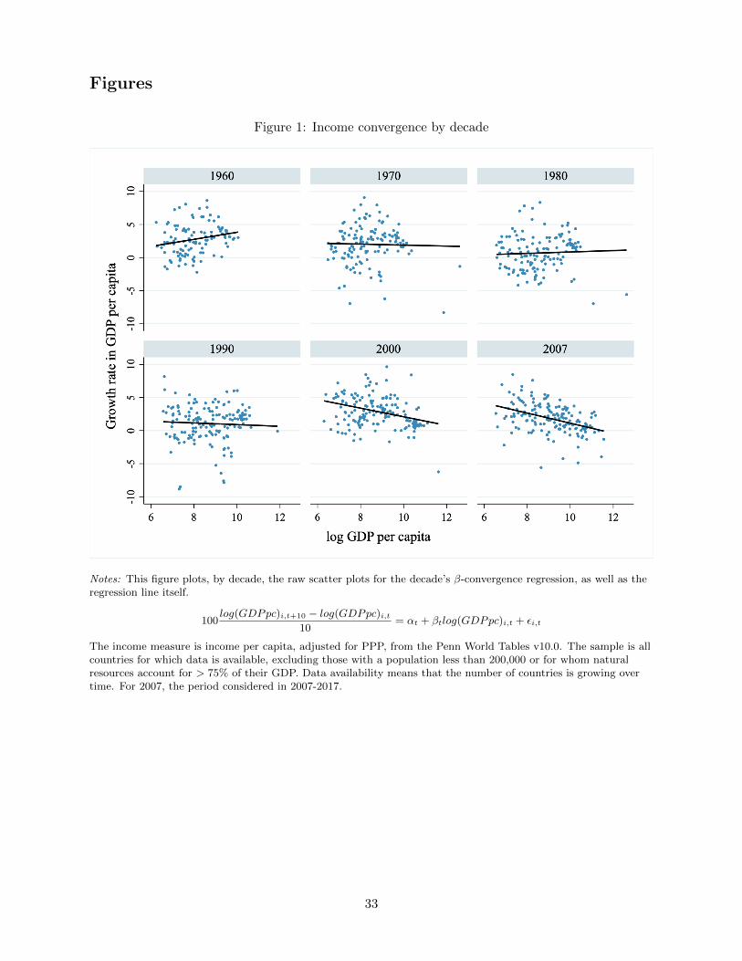
Figures
Figure 1: Income convergence by decade
Notes: This figure plots, by decade, the raw scatter plots for the decade’s β-convergence regression, as well as theregression line itself.
100log(GDPpc)i,t+10 − log(GDPpc)i,t
10= αt + βtlog(GDPpc)i,t + εi,t
The income measure is income per capita, adjusted for PPP, from the Penn World Tables v10.0. The sample is allcountries for which data is available, excluding those with a population less than 200,000 or for whom naturalresources account for > 75% of their GDP. Data availability means that the number of countries is growing overtime. For 2007, the period considered in 2007-2017.
33
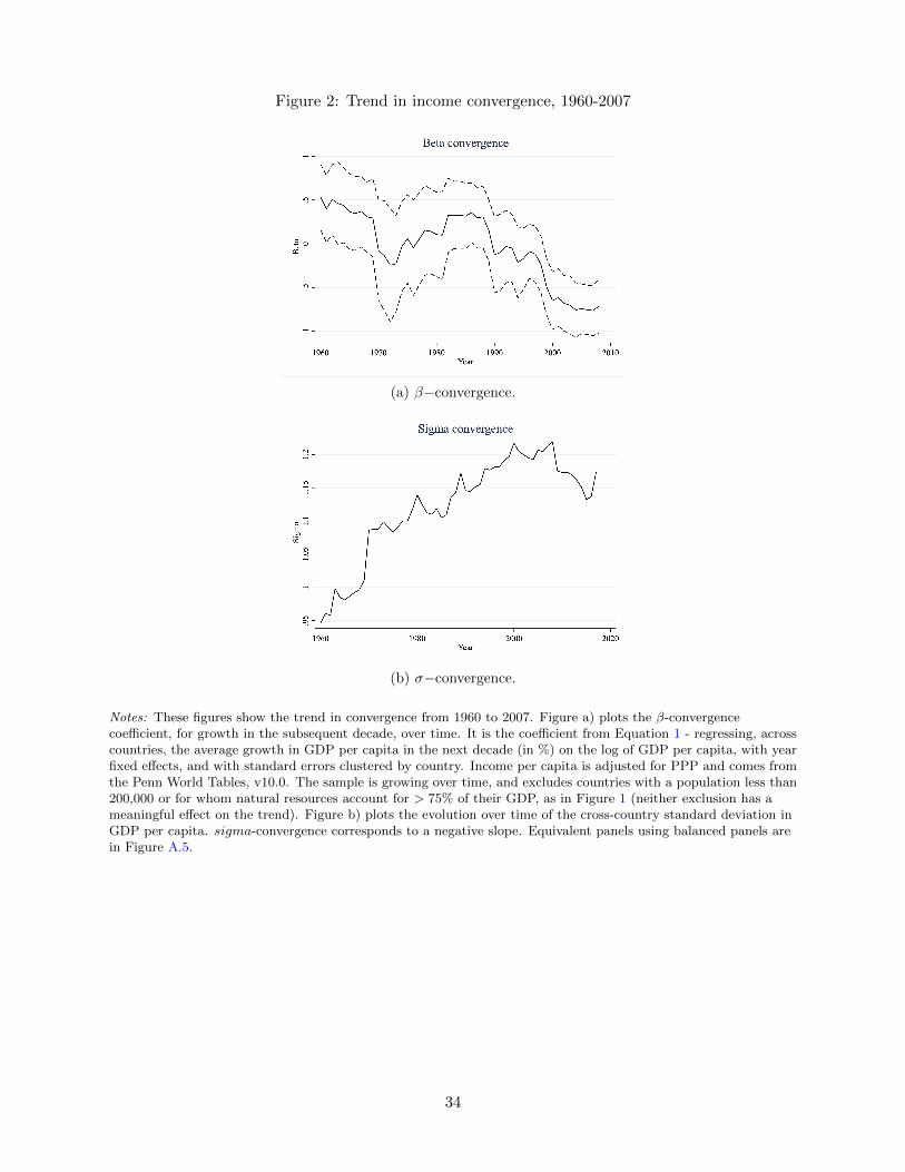
Figure 2: Trend in income convergence, 1960-2007
(a) β−convergence.
(b) σ−convergence.
Notes: These figures show the trend in convergence from 1960 to 2007. Figure a) plots the β-convergencecoefficient, for growth in the subsequent decade, over time. It is the coefficient from Equation 1 - regressing, acrosscountries, the average growth in GDP per capita in the next decade (in %) on the log of GDP per capita, with yearfixed effects, and with standard errors clustered by country. Income per capita is adjusted for PPP and comes fromthe Penn World Tables, v10.0. The sample is growing over time, and excludes countries with a population less than200,000 or for whom natural resources account for > 75% of their GDP, as in Figure 1 (neither exclusion has ameaningful effect on the trend). Figure b) plots the evolution over time of the cross-country standard deviation inGDP per capita. sigma-convergence corresponds to a negative slope. Equivalent panels using balanced panels arein Figure A.5.
34
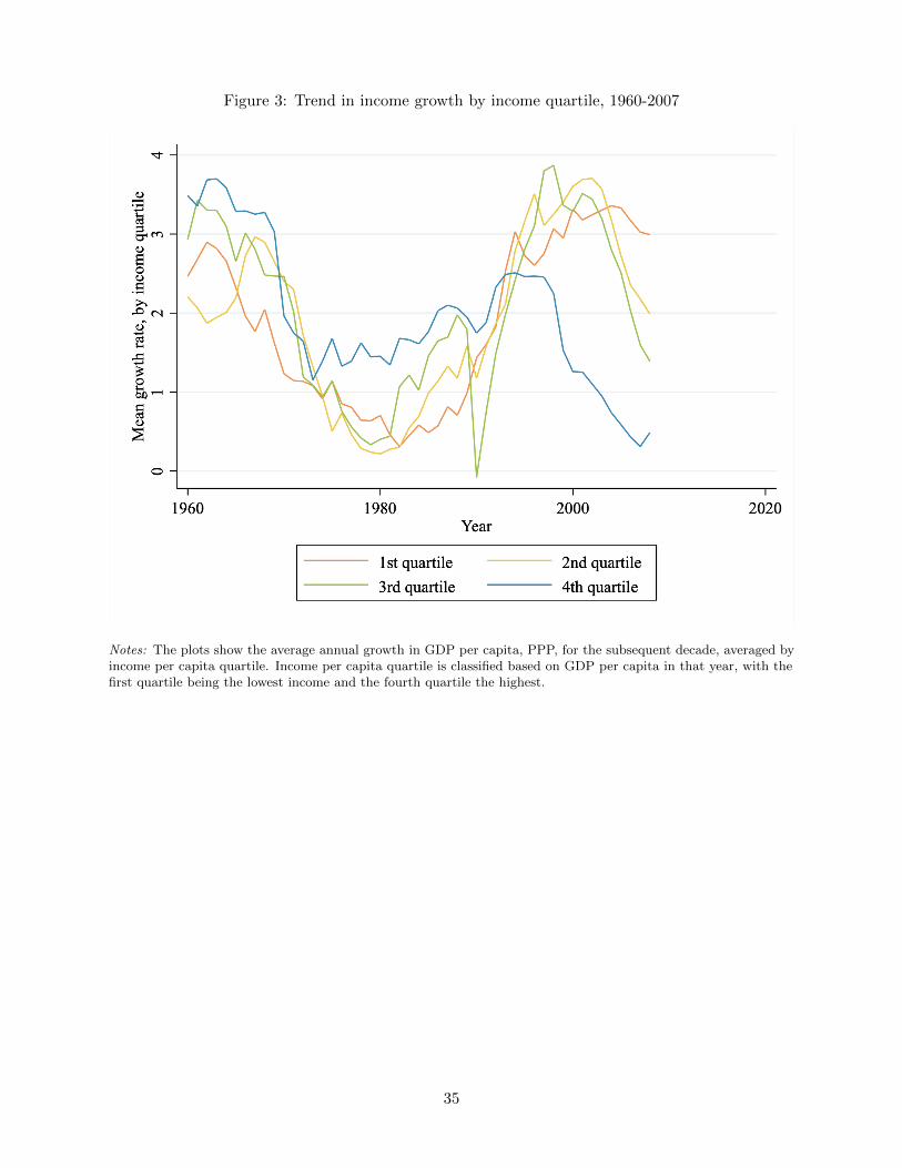
Figure 3: Trend in income growth by income quartile, 1960-2007
Notes: The plots show the average annual growth in GDP per capita, PPP, for the subsequent decade, averaged byincome per capita quartile. Income per capita quartile is classified based on GDP per capita in that year, with thefirst quartile being the lowest income and the fourth quartile the highest.
35
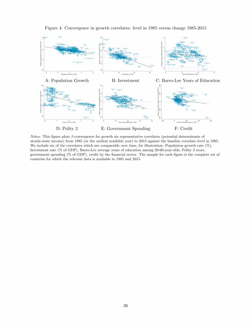
Figure 4: Convergence in growth correlates: level in 1985 versus change 1985-2015
Afghanistan
Angola
Albania
United Arab Emirates
ArgentinaArmenia
AustraliaAustria
AzerbaijanBurundiBelgium Benin
Burkina Faso
Bangladesh
BulgariaBahrain
Bahamas, The
Bosnia and Herzegovina
Belarus BelizeBoliviaBrazil
Barbados
BhutanBotswana
Central African Republic
CanadaSwitzerland
ChileChinaCote d'Ivoire
Cameroon
Congo, Dem. Rep.
Congo, Rep.Colombia
ComorosCabo Verde
Costa Rica
CubaCyprusCzech RepublicGermany
Djibouti
Denmark
Dominican RepublicAlgeriaEcuadorEgypt, Arab Rep.SpainEstonia Ethiopia
FinlandFiji
FranceGabonUnited Kingdom
Georgia
GhanaGuinea
Gambia, The
Guinea-Bissau
Equatorial GuineaGreece
Guatemala
Guyana
Hong Kong SAR, ChinaHonduras
Croatia HaitiHungary
IndonesiaIndia
Ireland
Iran, Islamic Rep.
Iceland IsraelItaly
Jamaica
Jordan
Japan
Kazakhstan
Kenya
Kyrgyz Republic
Cambodia
Korea, Rep.Kuwait
Lao PDR
Lebanon
Libya
Sri LankaLesotho
Lithuania
Luxembourg
Latvia Macao SAR, China
MoroccoMoldovaMadagascar
MaldivesMexicoNorth Macedonia
MaliMalta
MyanmarMontenegro Mongolia
Mozambique
MauritaniaMauritius
MalawiMalaysiaNamibia
New Caledonia
NigerNigeria
Nicaragua
Netherlands
Norway
Nepal
New Zealand
Oman
PakistanPanama
PeruPhilippinesPapua New GuineaPoland
Puerto Rico
PortugalParaguay
French Polynesia
RomaniaRussian Federation
RwandaSudan
Senegal
Singapore
Solomon IslandsSierra Leone
El Salvador
Somalia
South SudanSao Tome and PrincipeSuriname
Slovak RepublicSlovenia
Sweden
Eswatini
Syrian Arab Republic
Chad
TogoThailand
TajikistanTimor-LesteTrinidad and TobagoTunisia
TurkeyTanzaniaUganda
UkraineUruguayUnited States
UzbekistanVenezuela, RBVietnam
Vanuatu
Kosovo
Yemen, Rep.South Africa
Zambia
Zimbabwe
-10
-50
5C
hang
e in
Pop
ulat
ion
Gro
wth
(198
5-20
10)
-2 0 2 4 6Population Growth in 1985
A: Population Growth
Angola
Albania
Argentina AustraliaAustriaBurundiBelgium
Benin
Burkina Faso
Bangladesh
BulgariaBahrain
Bahamas, The
BelizeBoliviaBrazilBarbados
BhutanBotswana
Central African Republic
Canada
Switzerland
Chile ChinaCote d'Ivoire
Cameroon
Congo, Rep.
Colombia
ComorosCosta Rica
CubaCyprus
GermanyDenmark
Dominican RepublicAlgeriaEcuador
Egypt, Arab Rep.
Spain
Ethiopia
Finland
FijiFrance
GabonUnited Kingdom Georgia
Ghana
Guinea-BissauGreece
Guatemala
Guyana
Hong Kong SAR, ChinaHonduras
IndonesiaIndia
Ireland
Iran, Islamic Rep.
IcelandIsrael
ItalyJamaica
Jordan
JapanKenya Korea, Rep.Kuwait
Lao PDR
Sri Lanka
LuxembourgMacao SAR, China
MoroccoMadagascar
MexicoMali
Malta
Mongolia
Mozambique
Mauritania
MauritiusMalawi
Malaysia
NamibiaNiger
Nigeria
Nicaragua
NetherlandsNorway
Nepal
New ZealandOman
Pakistan
Panama
PeruPhilippines
Puerto RicoPortugal
ParaguayRwandaSudan Senegal
Singapore
Sierra LeoneEl Salvador
Sweden
Eswatini
Chad
Togo
ThailandTunisia
Turkey
Uganda
Uruguay
United States
Venezuela, RB
VanuatuSouth Africa
Zimbabwe
-40
-20
020
4060
Cha
nge
in In
vest
men
t (19
85-2
010)
0 20 40 60Investment in 1985
B: Investment
Afghanistan
Albania
United Arab Emirates
Argentina
Armenia
Australia
Austria
Burundi
Belgium
Benin
Bangladesh
Bulgaria
Bahrain
Belize
Bolivia
Brazil
Barbados
Botswana
Central African Republic
CanadaSwitzerland
Chile
China
Cote d'IvoireCameroon
Congo, Dem. Rep.Congo, Rep.
Colombia
Costa Rica
CubaCyprus
Czech Republic
Germany
Denmark
Dominican Republic
Algeria
Ecuador
Egypt, Arab Rep.Spain
EstoniaFinland
Fiji
FranceGabon
United Kingdom
GhanaGambia, The
Greece
GuatemalaGuyana
Hong Kong SAR, China
Honduras
CroatiaHaiti
Hungary
Indonesia
India
Ireland
Iran, Islamic Rep.
Iceland
Israel
Italy
JamaicaJordan
Japan
KazakhstanKenya
Kyrgyz RepublicCambodia
Korea, Rep.
Kuwait
Lao PDR
Libya
Sri Lanka
Lesotho
LithuaniaLuxembourg
LatviaMacao SAR, China
Morocco
Maldives
Mexico
Mali
Malta
Myanmar Mongolia
Mozambique
Mauritania
Mauritius
Malawi
Malaysia
NamibiaNiger
Nicaragua
Netherlands
Norway
Nepal
New Zealand
Pakistan Panama
Peru
PhilippinesPapua New Guinea
PolandPortugal
ParaguayRomania
Russian Federation
RwandaSudan
Senegal
Singapore
Sierra Leone
El Salvador
Slovak RepublicSlovenia
Sweden
Eswatini
Syrian Arab Republic
Togo
Thailand
Tajikistan
Trinidad and Tobago
Tunisia
Turkey
Tanzania
Uganda
Ukraine
Uruguay
United States
Venezuela, RB
VietnamYemen, Rep.
South Africa
Zambia
Zimbabwe
02
46
Cha
nge
in Y
ears
of E
duca
tion
(198
5-20
10)
0 5 10 15Years of Education in 1985
C: Barro-Lee Years of Education
Angola
Albania
United Arab EmiratesArgentina
AustraliaAustria
Burundi
Belgium
BeninBurkina Faso
Bangladesh
Bulgaria
Bahrain
Bolivia
Brazil
Bhutan
Botswana
Central African Republic
CanadaSwitzerland
Chile
China
Cameroon
Congo, Dem. Rep.
Congo, Rep.
Colombia
Comoros
Cabo Verde
Costa RicaCuba Cyprus
Czech Republic
Germany
Djibouti
Denmark
Dominican Republic
Algeria
Ecuador
Egypt, Arab Rep.
Spain
Ethiopia
Finland
Fiji
France
Gabon
United Kingdom
Ghana
Guinea
Gambia, The
Guinea-Bissau
Equatorial GuineaGreece
Guatemala
Guyana
Honduras
Haiti
HungaryIndonesia
IndiaIreland
Iran, Islamic Rep.Israel Italy
Jamaica
Jordan
Japan
Kenya
Korea, Rep.
KuwaitLao PDR
LebanonLibya
Sri Lanka
Lesotho
Luxembourg
Morocco
MadagascarMexico
Mali
Myanmar
Mongolia
Mozambique
Mauritania
Mauritius
Malawi
Malaysia
NigerNigeria
Nicaragua
NetherlandsNorway
Nepal
New Zealand
Oman
Pakistan
Panama
Peru
Philippines
Papua New Guinea
Poland
Portugal
ParaguayRomania
Rwanda
Sudan
Senegal
SingaporeSolomon Islands
Sierra Leone
El Salvador
SomaliaSerbia
Suriname
SwedenEswatini
Syrian Arab Republic
ChadTogo
Thailand
Trinidad and Tobago
Tunisia
Turkey
Tanzania
Uganda
UruguayUnited States
Venezuela, RB
Vietnam
South Africa
Zambia
Zimbabwe
-10
010
20C
hang
e in
Pol
ity 2
Sco
re (1
985-
2015
)
-10 -5 0 5 10Polity 2 Score in 1985
D: Polity 2
AlbaniaAustraliaAustria
Burundi
BelgiumBenin
Burkina Faso
BangladeshBulgaria
Bahrain
Bahamas, The
Belize
Bolivia
Brazil
Barbados Bhutan
Botswana
Central African Republic
Canada
SwitzerlandChileChina
Cote d'Ivoire
CameroonCongo, Rep.
Colombia
Comoros
Costa Rica CubaCyprus
GermanyDenmark
Dominican Republic Algeria
Ecuador
Egypt, Arab Rep.
Spain Finland
Fiji France
Gabon
United Kingdom
Georgia
Ghana
Gambia, TheGuinea-Bissau
GreeceGuatemala
Guyana
Hong Kong SAR, China
IndonesiaIndia
Ireland
Iran, Islamic Rep.
Iceland
Israel
ItalyJamaica
Jordan
Japan
Kenya
Korea, Rep.
Kuwait
Lao PDR
Sri LankaLuxembourg
Macao SAR, China MoroccoMadagascar
Mexico
Mali
Malta
Mongolia
Mozambique
Mauritania
Mauritius
MalawiMalaysia
Namibia
NigerNigeria
Nicaragua
Netherlands
Norway
Nepal New Zealand OmanPakistan
Panama
PeruPhilippines
Puerto Rico
PortugalParaguayRwanda
Sudan
SenegalSingapore
Sierra LeoneEl Salvador SwedenEswatini
Chad
TogoThailand
Tunisia
Turkey
Uganda
UruguayUnited States
Venezuela, RB
Vanuatu
South Africa
Zimbabwe-2
0-1
00
1020
Cha
nge
in G
over
nmen
t Spe
ndin
g (1
985-
2015
)
0 10 20 30 40Government Spending in 1985
E: Government Spending
United Arab Emirates
Argentina
Australia
BurundiBeninBurkina Faso
Bangladesh
Bahrain
Bahamas, TheBelize
Bolivia
Brazil
BhutanBotswana
Central African Republic Switzerland
Chile
China
Cote d'IvoireCameroon
Congo, Dem. Rep.Congo, Rep.ColombiaComoros
Cabo VerdeCosta Rica
Djibouti
Denmark
Dominican Republic
Algeria
Ecuador
Egypt, Arab Rep.
Fiji
Gabon
United Kingdom
GhanaGambia, The
Guinea-BissauEquatorial Guinea
Guatemala
Guyana
Hong Kong SAR, China
HondurasHaitiIndonesia
IndiaIran, Islamic Rep.
Iceland
IsraelJamaica
Jordan
Japan
Kenya
Korea, Rep.
Lao PDR
Lebanon
Libya
Sri Lanka
Lesotho
Macao SAR, China
Morocco
Madagascar
MaldivesMexicoMali
Myanmar
Mozambique
Mauritania
Mauritius
Malawi
MalaysiaNamibia
NigerNigeria
Nicaragua
Norway
Nepal
New Zealand
Oman
Pakistan
Panama
PeruPhilippines
Papua New Guinea
Poland
Paraguay
Romania
RwandaSudan
Senegal
Singapore
Solomon IslandsSierra Leone
El Salvador
Suriname
Sweden
EswatiniChad
Togo
Thailand
Trinidad and Tobago
Tunisia
Turkey
TanzaniaUruguay
United States
Venezuela, RBVanuatu
Yemen, Rep.
South Africa
Zambia
-200
-100
010
020
0C
hang
e in
Cre
dit b
y Fi
nanc
ial S
ecto
r (19
90-2
015)
-100 0 100 200 300Credit by Financial Sector in 1990
F: Credit
Notes: This figure plots β-convergence for growth six representative correlates (potential determinants ofsteady-state income) from 1985 (or the earliest available year) to 2015 against the baseline correlate level in 1985.We include six of the correlates which are comparable over time, for illustration: Population growth rate (%),Investment rate (% of GDP), Barro-Lee average years of education among 20-60-year-olds, Polity 2 score,government spending (% of GDP), credit by the financial sector. The sample for each figure is the complete set ofcountries for which the relevant data is available in 1985 and 2015.
36
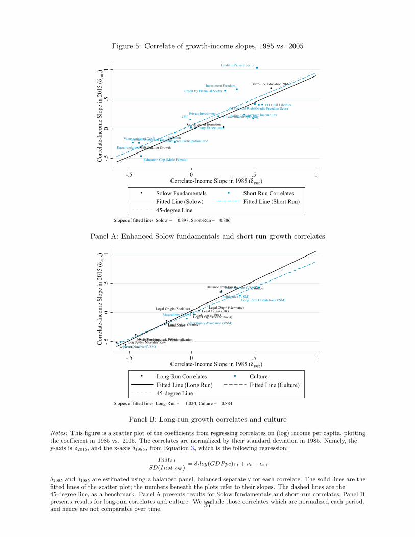
Figure 5: Correlate of growth-income slopes, 1985 vs. 2005
Education Gap (Male-Female)
Labor Force Participation Rate
Polity 2 Score
FH Political RightsFH Civil Liberties
Media Freedom Score
Equal-weighted Tariff
Value-weighted Tariff
Average Income Tax
Taxes on Goods and Services
Government SpendingPrivate Investment
Military Expenditure
Inflation
CBI
Credit to Private Sector
Credit by Financial SectorInvestment Freedom
Gross capital formation
Population Growth
Barro-Lee Education 20-60
-.50
.51
Cor
rela
te-I
ncom
e Sl
ope
in 2
015
(δ20
15)
-.5 0 .5 1Correlate-Income Slope in 1985 (δ1985)
Solow Fundamentals Short Run CorrelatesFitted Line (Solow) Fitted Line (Short Run)45-degree Line
Slopes of fitted lines: Solow = 0.897; Short-Run = 0.886
Panel A: Enhanced Solow fundamentals and short-run growth correlates
Power Distance (VSM)
Individualism (VSM)
Masculinity (VSM)
Uncertainty Avoidance (VSM)
Indulgence (VSM)Long Term Orientation (VSM)
Population in 1900Legal Origin (UK)
Legal Origin (France)
Legal Origin (Germany)
Legal Origin (Scandinavia)
Legal Origin (Socialist)
Log Settler Mortality RateMean Temperature (1986)
Distance from Coast
Ethno-Linguistic Fractionalization
Landlocked
Latitude
Tropical Climate
-.50
.51
Cor
rela
te-I
ncom
e Sl
ope
in 2
015
(δ20
15)
-.5 0 .5 1Correlate-Income Slope in 1985 (δ1985)
Long Run Correlates CultureFitted Line (Long Run) Fitted Line (Culture)45-degree Line
Slopes of fitted lines: Long-Run = 1.024; Culture = 0.884
Panel B: Long-run growth correlates and culture
Notes: This figure is a scatter plot of the coefficients from regressing correlates on (log) income per capita, plottingthe coefficient in 1985 vs. 2015. The correlates are normalized by their standard deviation in 1985. Namely, they-axis is δ2015, and the x-axis δ1985, from Equation 3, which is the following regression:
Insti,tSD(Inst1985)
= δtlog(GDPpc)i,t + νt + εt,i
δ1985 and δ1985 are estimated using a balanced panel, balanced separately for each correlate. The solid lines are thefitted lines of the scatter plot; the numbers beneath the plots refer to their slopes. The dashed lines are the45-degree line, as a benchmark. Panel A presents results for Solow fundamentals and short-run correlates; Panel Bpresents results for long-run correlates and culture. We exclude those correlates which are normalized each period,and hence are not comparable over time.
37
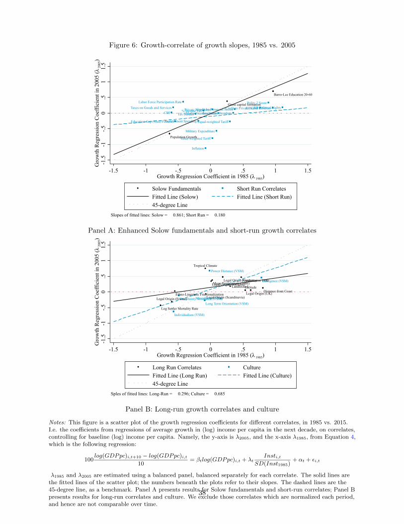
Figure 6: Growth-correlate of growth slopes, 1985 vs. 2005
Polity 2 Score
Education Gap (Male-Female)
Labor Force Participation RateFH Political RightsFH Civil Liberties
Media Freedom Score
Equal-weighted Tariff
Value-weighted Tariff
% Income TaxTaxes on Goods and Services
Government Spending
Tax BurdenPrivate Investment
Military Expenditure
Inflation
CBICredit to Private SectorCredit by Financial Sector
Investment Freedom
Gross capital formation
Population Growth
Barro-Lee Education 20-60
-1.5
-1-.5
0.5
11.
5G
row
th R
egre
ssio
n C
oeff
icie
nt in
200
5 (λ
200
5)
-1.5 -1 -.5 0 .5 1 1.5Growth Regression Coefficient in 1985 (λ 1985)
Solow Fundamentals Short Run CorrelatesFitted Line (Solow) Fitted Line (Short Run)45-degree Line
Slopes of fitted lines: Solow = 0.861; Short Run = 0.180
Panel A: Enhanced Solow fundamentals and short-run growth correlates
Power Distance (VSM)
Individualism (VSM)
Masculinity (VSM)Uncertainty Avoidance (VSM)
Indulgence (VSM)
Long Term Orientation (VSM)
Population in 1900
Legal Origin (UK)Legal Origin (France)
Legal Origin (Germany)
Legal Origin (Scandinavia)
Legal Origin (Socialist)
Log Settler Mortality Rate
Mean Temperature (1986)
Distance from CoastEthno-Linguistic Fractionalization
LandlockedLatitude
Tropical Climate
-1.5
-1-.5
0.5
11.
5G
row
th R
egre
ssio
n C
oeffi
cien
t in
2005
(λ 2
005)
-1.5 -1 -.5 0 .5 1 1.5Growth Regression Coefficient in 1985 (λ 1985)
Long Run Correlates CultureFitted Line (Long Run) Fitted Line (Culture)45-degree Line
Sples of fitted lines: Long-Run = 0.296; Culture = 0.685
Panel B: Long-run growth correlates and culture
Notes: This figure is a scatter plot of the growth regression coefficients for different correlates, in 1985 vs. 2015.I.e. the coefficients from regressions of average growth in (log) income per capita in the next decade, on correlates,controlling for baseline (log) income per capita. Namely, the y-axis is λ2005, and the x-axis λ1985, from Equation 4,which is the following regression:
100log(GDPpc)i,t+10 − log(GDPpc)i,t
10= βtlog(GDPpc)i,t + λt
Insti,tSD(Inst1985)
+ αt + εi,t
λ1985 and λ2005 are estimated using a balanced panel, balanced separately for each correlate. The solid lines arethe fitted lines of the scatter plot; the numbers beneath the plots refer to their slopes. The dashed lines are the45-degree line, as a benchmark. Panel A presents results for Solow fundamentals and short-run correlates; Panel Bpresents results for long-run correlates and culture. We exclude those correlates which are normalized each period,and hence are not comparable over time.
38
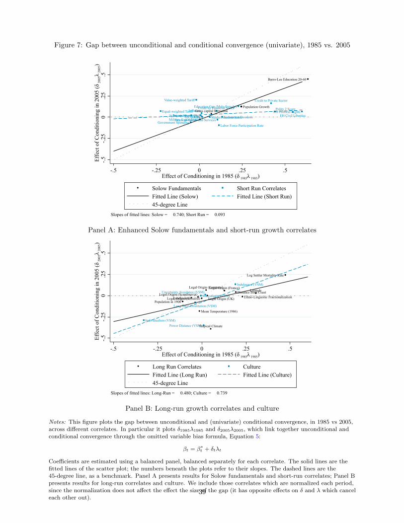
Figure 7: Gap between unconditional and conditional convergence (univariate), 1985 vs. 2005
Polity 2 ScoreEducation Gap (Male-Female)
Labor Force Participation Rate
FH Political RightsFH Civil LibertiesMedia Freedom Score
Equal-weighted Tariff
Value-weighted Tariff
% Income TaxTaxes on Goods and Services
Government SpendingTax BurdenPrivate Investment
Military Expenditure
Inflation
CBI
Credit to Private Sector
Credit by Financial Sector
Investment Freedom
Gross capital formationPopulation Growth
Barro-Lee Education 20-60
-.5-.2
50
.25
.5Ef
fect
of C
ondi
tioni
ng in
200
5 (δ
200
5λ 2
005)
-.5 -.25 0 .25 .5Effect of Conditioning in 1985 (δ 1985λ 1985)
Solow Fundamentals Short Run CorrelatesFitted Line (Solow) Fitted Line (Short Run)45-degree Line
Slopes of fitted lines: Solow = 0.740; Short Run = 0.093
Panel A: Enhanced Solow fundamentals and short-run growth correlates
Power Distance (VSM)Individualism (VSM)
Masculinity (VSM)Uncertainty Avoidance (VSM)
Indulgence (VSM)
Long Term Orientation (VSM)Population in 1900
Legal Origin (UK)
Legal Origin (France)Legal Origin (Germany)
Legal Origin (Scandinavia)Legal Origin (Socialist)
Log Settler Mortality Rate
Mean Temperature (1986)
Distance from CoastEthno-Linguistic FractionalizationLandlocked
Latitude
Tropical Climate
-.5-.2
50
.25
.5Ef
fect
of C
ondi
tioni
ng in
200
5 (δ
200
5λ 2
005)
-.5 -.25 0 .25 .5Effect of Conditioning in 1985 (δ 1985λ 1985)
Long Run Correlates CultureFitted Line (Long Run) Fitted Line (Culture)45-degree Line
Slopes of fitted lines: Long-Run = 0.480; Culture = 0.739
Panel B: Long-run growth correlates and culture
Notes: This figure plots the gap between unconditional and (univariate) conditional convergence, in 1985 vs 2005,across different correlates. In particular it plots δ1985λ1985 and δ2005λ2005, which link together unconditional andconditional convergence through the omitted variable bias formula, Equation 5:
βt = β∗t + δtλt
Coefficients are estimated using a balanced panel, balanced separately for each correlate. The solid lines are thefitted lines of the scatter plot; the numbers beneath the plots refer to their slopes. The dashed lines are the45-degree line, as a benchmark. Panel A presents results for Solow fundamentals and short-run correlates; Panel Bpresents results for long-run correlates and culture. We include those correlates which are normalized each period,since the normalization does not affect the effect the size of the gap (it has opposite effects on δ and λ which canceleach other out).
39
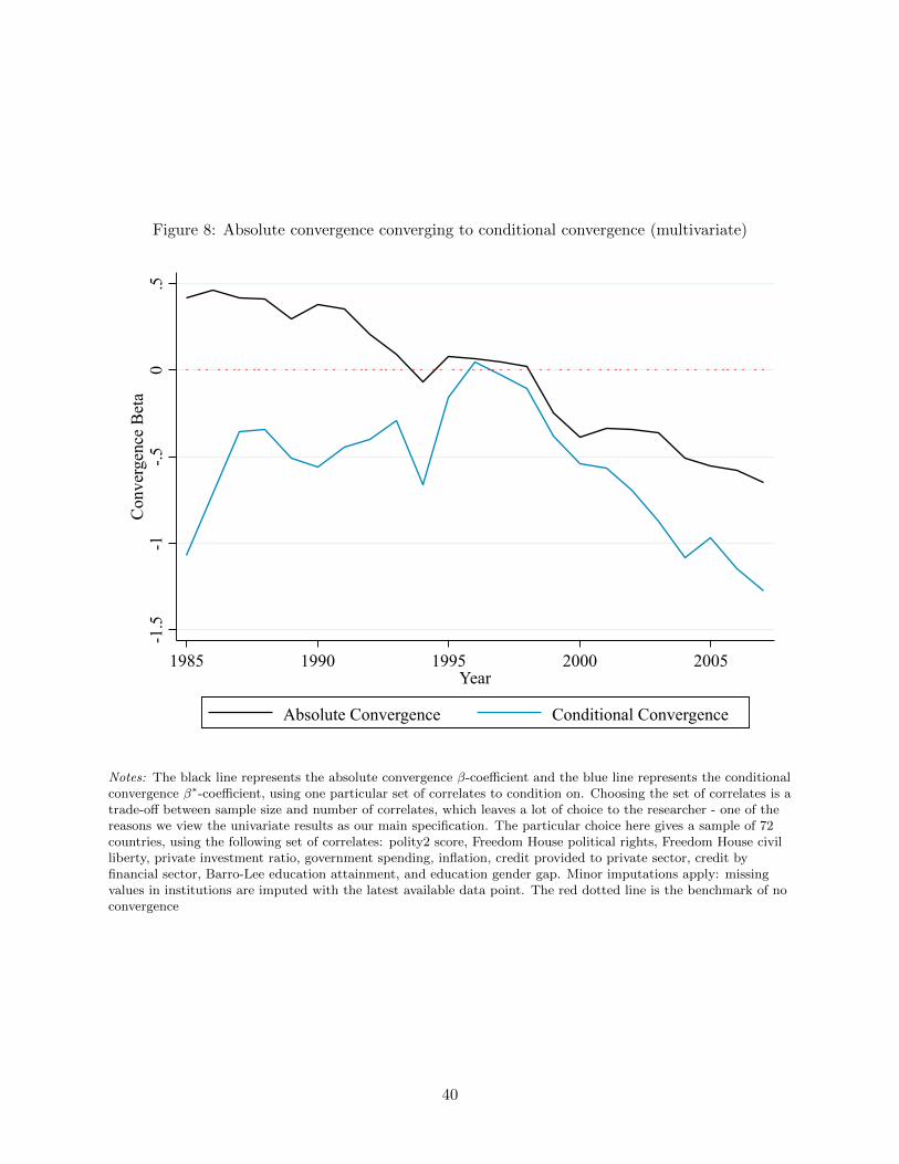
Figure 8: Absolute convergence converging to conditional convergence (multivariate)
-1.5
-1-.5
0.5
Con
verg
ence
Bet
a
1985 1990 1995 2000 2005Year
Absolute Convergence Conditional Convergence
Notes: The black line represents the absolute convergence β-coefficient and the blue line represents the conditionalconvergence β∗-coefficient, using one particular set of correlates to condition on. Choosing the set of correlates is atrade-off between sample size and number of correlates, which leaves a lot of choice to the researcher - one of thereasons we view the univariate results as our main specification. The particular choice here gives a sample of 72countries, using the following set of correlates: polity2 score, Freedom House political rights, Freedom House civilliberty, private investment ratio, government spending, inflation, credit provided to private sector, credit byfinancial sector, Barro-Lee education attainment, and education gender gap. Minor imputations apply: missingvalues in institutions are imputed with the latest available data point. The red dotted line is the benchmark of noconvergence
40
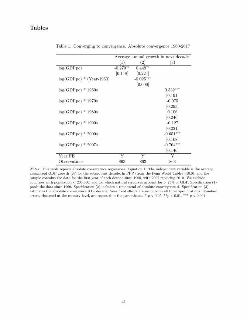
Tables
Table 1: Converging to convergence. Absolute convergence 1960-2017
Average annual growth in next decade(1) (2) (3)
log(GDPpc) -0.270∗∗ 0.449∗∗
[0.118] [0.224]log(GDPpc) * (Year-1960) -0.025∗∗∗
[0.006]log(GDPpc) * 1960s 0.532∗∗∗
[0.191]log(GDPpc) * 1970s -0.075
[0.293]log(GDPpc) * 1980s 0.106
[0.246]log(GDPpc) * 1990s -0.127
[0.221]log(GDPpc) * 2000s -0.651∗∗∗
[0.168]log(GDPpc) * 2007s -0.764∗∗∗
[0.146]
Year FE Y Y YObservations 863 863 863
Notes: This table reports absolute convergence regressions, Equation 1. The independent variable is the averageannualized GDP growth (%) for the subsequent decade, in PPP (from the Penn World Tables v10.0), and thesample contains the data for the first year of each decade since 1960, with 2007 replacing 2010. We excludecountries with population < 200,000, and for which natural resources account for > 75% of GDP. Specification (1)pools the data since 1960. Specification (2) includes a time trend of absolute convergence β. Specification (3)estimates the absolute convergence β by decade. Year fixed effects are included in all three specifications. Standarderrors, clustered at the country-level, are reported in the parentheses. * p < 0.05, **p < 0.01, *** p < 0.001
41
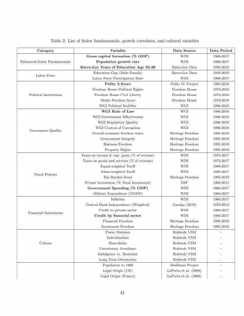
Table 2: List of Solow fundamentals, growth correlates, and cultural variables
Category Variable Data Source Data Period
Enhanced Solow Fundamentals
Gross capital formation (% GDP) WDI 1960-2017
Population growth rate WDI 1960-2017
Barro-Lee Years of Education Age 25-29 Barro-Lee Data 1950-2010
Labor ForceEducation Gap (Male-Female) Barro-Lee Data 1950-2010
Labor Force Participation Rate WDI 1960-2017
Political Institutions
Polity 2 Score Polity IV Project 1960-2018
Freedom House Political Rights Freedom House 1973-2018
Freedom House Civil Liberty Freedom House 1973-2018
Media Freedom Score Freedom House 1979-2018
WGI Political Stability WGI 1996-2018
Governance Quality
WGI Rule of Law WGI 1996-2018
WGI Government Effectiveness WGI 1996-2018
WGI Regulatory Quality WGI 1996-2018
WGI Control of Corruption WGI 1996-2018
Overall economic freedom index Heritage Freedom 1995-2019
Government Integrity Heritage Freedom 1995-2019
Business Freedom Heritage Freedom 1995-2019
Property Rights Heritage Freedom 1995-2019
Fiscal Policies
Taxes on income & cap. gains (% of revenue) WDI 1972-2017
Taxes on goods and services (% of revenue) WDI 1972-2017
Equal-weighted Tariff WDI 1988-2017
Value-weighted Tariff WDI 1988-2017
Tax Burden Score Heritage Freedom 1995-2019
Private Investment (% Total Investment) IMF 1960-2015
Government Spending (% GDP) WDI 1960-2017
Military Expenditure (%GDP) WDI 1960-2017
Financial Institutions
Inflation WDI 1960-2017
Central Bank Independence (Weighted) Garriga (2019) 1970-2012
Credit to private sector WDI 1960-2017
Credit by financial sector WDI 1960-2017
Financial Freedom Heritage Freedom 1995-2019
Investment Freedom Heritage Freedom 1995-2019
Power Distance Hofstede VSM -
Individualism Hofstede VSM -
Culture Masculinity Hofstede VSM -
Uncertainty Avoidance Hofstede VSM -
Indulgence vs. Restraint Hofstede VSM -
Long Term Orientation Hofstede VSM -
Population in 1900 Maddison Project -
Legal Origin (UK) LaPorta et al. (2008) -
Legal Origin (France) LaPorta et al. (2008) -
42
Legal Origin (Germany) LaPorta et al. (2008) -
Legal Origin (Scandinavia) LaPorta et al. (2008) -
Long-Run Variables Legal Origin (Socialist) LaPorta et al. (2008) -
Log Settler Mortality Rate Acemoglu et al. (2001) -
Mean Temperature Acemoglu et al. (2001) -
100km of the Coastline Acemoglu et al. (2001) -
Ethno-Linguistic Fractionalization Acemoglu et al. (2001) -
Landlocked Acemoglu et al. (2001) -
Absolute Latitude Acemoglu et al. (2001) -
Tropical Climate Sachs and Warner
(1997a)
-
This table summarizes all enhanced Solow fundamentals, growth coorelates, and cultural variables considered in the analysis, which
we divide into four broad groups: enhanced Solow fundamentals, short-run correlates (comprising political institutions, governance,
fiscal policy, financial institutions), long-run correlates, and culture. Columns 3 and 4 report the data source and data period for
each variable. The variables in bold are the representative correlates reported in Figure A.14 and Figure 4. Some of the correlates
are not directly comparable across time, for example the WGI indicators are standardized each year. In subsequent analysis we
only consider such variables for conditional versus absolute convergence, where such standardization does not matter.
43
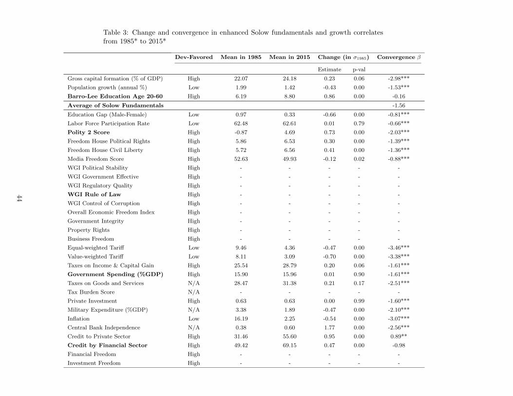
Table 3: Change and convergence in enhanced Solow fundamentals and growth correlatesfrom 1985* to 2015*
Dev-Favored Mean in 1985 Mean in 2015 Change (in σ1985) Convergence β
Estimate p-val
Gross capital formation (% of GDP) High 22.07 24.18 0.23 0.06 -2.98***
Population growth (annual %) Low 1.99 1.42 -0.43 0.00 -1.53***
Barro-Lee Education Age 20-60 High 6.19 8.80 0.86 0.00 -0.16
Average of Solow Fundamentals -1.56
Education Gap (Male-Female) Low 0.97 0.33 -0.66 0.00 -0.81***
Labor Force Participation Rate Low 62.48 62.61 0.01 0.79 -0.66***
Polity 2 Score High -0.87 4.69 0.73 0.00 -2.03***
Freedom House Political Rights High 5.86 6.53 0.30 0.00 -1.39***
Freedom House Civil Liberty High 5.72 6.56 0.41 0.00 -1.36***
Media Freedom Score High 52.63 49.93 -0.12 0.02 -0.88***
WGI Political Stability High - - - - -
WGI Government Effective High - - - - -
WGI Regulatory Quality High - - - - -
WGI Rule of Law High - - - - -
WGI Control of Corruption High - - - - -
Overall Economic Freedom Index High - - - - -
Government Integrity High - - - - -
Property Rights High - - - - -
Business Freedom High - - - - -
Equal-weighted Tariff Low 9.46 4.36 -0.47 0.00 -3.46***
Value-weighted Tariff Low 8.11 3.09 -0.70 0.00 -3.38***
Taxes on Income & Capital Gain High 25.54 28.79 0.20 0.06 -1.61***
Government Spending (%GDP) High 15.90 15.96 0.01 0.90 -1.61***
Taxes on Goods and Services N/A 28.47 31.38 0.21 0.17 -2.51***
Tax Burden Score N/A - - - - -
Private Investment High 0.63 0.63 0.00 0.99 -1.60***
Military Expenditure (%GDP) N/A 3.38 1.89 -0.47 0.00 -2.10***
Inflation Low 16.19 2.25 -0.54 0.00 -3.07***
Central Bank Independence N/A 0.38 0.60 1.77 0.00 -2.56***
Credit to Private Sector High 31.46 55.60 0.95 0.00 0.89**
Credit by Financial Sector High 49.42 69.15 0.47 0.00 -0.98
Financial Freedom High - - - - -
Investment Freedom High - - - - -
44
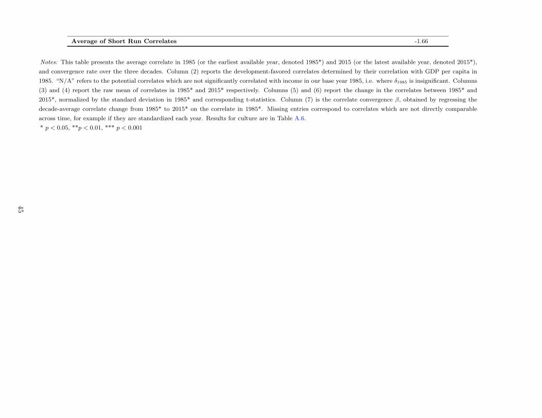
Average of Short Run Correlates -1.66
Notes: This table presents the average correlate in 1985 (or the earliest available year, denoted 1985*) and 2015 (or the latest available year, denoted 2015*),
and convergence rate over the three decades. Column (2) reports the development-favored correlates determined by their correlation with GDP per capita in
1985. “N/A” refers to the potential correlates which are not significantly correlated with income in our base year 1985, i.e. where δ1985 is insignificant. Columns
(3) and (4) report the raw mean of correlates in 1985* and 2015* respectively. Columns (5) and (6) report the change in the correlates between 1985* and
2015*, normalized by the standard deviation in 1985* and corresponding t-statistics. Column (7) is the correlate convergence β, obtained by regressing the
decade-average correlate change from 1985* to 2015* on the correlate in 1985*. Missing entries correspond to correlates which are not directly comparable
across time, for example if they are standardized each year. Results for culture are in Table A.6.
* p < 0.05, **p < 0.01, *** p < 0.001
45
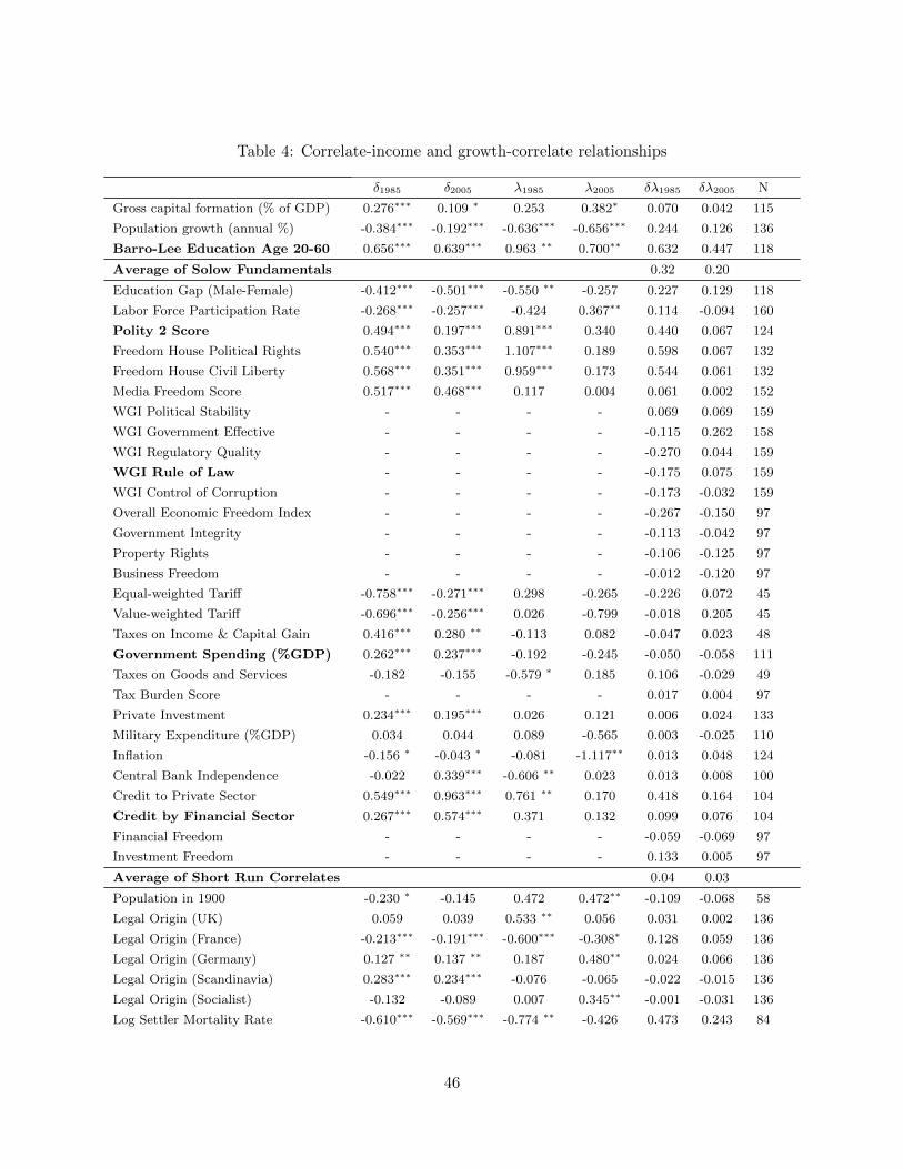
Table 4: Correlate-income and growth-correlate relationships
δ1985 δ2005 λ1985 λ2005 δλ1985 δλ2005 N
Gross capital formation (% of GDP) 0.276∗∗∗ 0.109 ∗ 0.253 0.382∗ 0.070 0.042 115
Population growth (annual %) -0.384∗∗∗ -0.192∗∗∗ -0.636∗∗∗ -0.656∗∗∗ 0.244 0.126 136
Barro-Lee Education Age 20-60 0.656∗∗∗ 0.639∗∗∗ 0.963 ∗∗ 0.700∗∗ 0.632 0.447 118
Average of Solow Fundamentals 0.32 0.20
Education Gap (Male-Female) -0.412∗∗∗ -0.501∗∗∗ -0.550 ∗∗ -0.257 0.227 0.129 118
Labor Force Participation Rate -0.268∗∗∗ -0.257∗∗∗ -0.424 0.367∗∗ 0.114 -0.094 160
Polity 2 Score 0.494∗∗∗ 0.197∗∗∗ 0.891∗∗∗ 0.340 0.440 0.067 124
Freedom House Political Rights 0.540∗∗∗ 0.353∗∗∗ 1.107∗∗∗ 0.189 0.598 0.067 132
Freedom House Civil Liberty 0.568∗∗∗ 0.351∗∗∗ 0.959∗∗∗ 0.173 0.544 0.061 132
Media Freedom Score 0.517∗∗∗ 0.468∗∗∗ 0.117 0.004 0.061 0.002 152
WGI Political Stability - - - - 0.069 0.069 159
WGI Government Effective - - - - -0.115 0.262 158
WGI Regulatory Quality - - - - -0.270 0.044 159
WGI Rule of Law - - - - -0.175 0.075 159
WGI Control of Corruption - - - - -0.173 -0.032 159
Overall Economic Freedom Index - - - - -0.267 -0.150 97
Government Integrity - - - - -0.113 -0.042 97
Property Rights - - - - -0.106 -0.125 97
Business Freedom - - - - -0.012 -0.120 97
Equal-weighted Tariff -0.758∗∗∗ -0.271∗∗∗ 0.298 -0.265 -0.226 0.072 45
Value-weighted Tariff -0.696∗∗∗ -0.256∗∗∗ 0.026 -0.799 -0.018 0.205 45
Taxes on Income & Capital Gain 0.416∗∗∗ 0.280 ∗∗ -0.113 0.082 -0.047 0.023 48
Government Spending (%GDP) 0.262∗∗∗ 0.237∗∗∗ -0.192 -0.245 -0.050 -0.058 111
Taxes on Goods and Services -0.182 -0.155 -0.579 ∗ 0.185 0.106 -0.029 49
Tax Burden Score - - - - 0.017 0.004 97
Private Investment 0.234∗∗∗ 0.195∗∗∗ 0.026 0.121 0.006 0.024 133
Military Expenditure (%GDP) 0.034 0.044 0.089 -0.565 0.003 -0.025 110
Inflation -0.156 ∗ -0.043 ∗ -0.081 -1.117∗∗ 0.013 0.048 124
Central Bank Independence -0.022 0.339∗∗∗ -0.606 ∗∗ 0.023 0.013 0.008 100
Credit to Private Sector 0.549∗∗∗ 0.963∗∗∗ 0.761 ∗∗ 0.170 0.418 0.164 104
Credit by Financial Sector 0.267∗∗∗ 0.574∗∗∗ 0.371 0.132 0.099 0.076 104
Financial Freedom - - - - -0.059 -0.069 97
Investment Freedom - - - - 0.133 0.005 97
Average of Short Run Correlates 0.04 0.03
Population in 1900 -0.230 ∗ -0.145 0.472 0.472∗∗ -0.109 -0.068 58
Legal Origin (UK) 0.059 0.039 0.533 ∗∗ 0.056 0.031 0.002 136
Legal Origin (France) -0.213∗∗∗ -0.191∗∗∗ -0.600∗∗∗ -0.308∗ 0.128 0.059 136
Legal Origin (Germany) 0.127 ∗∗ 0.137 ∗∗ 0.187 0.480∗∗ 0.024 0.066 136
Legal Origin (Scandinavia) 0.283∗∗∗ 0.234∗∗∗ -0.076 -0.065 -0.022 -0.015 136
Legal Origin (Socialist) -0.132 -0.089 0.007 0.345∗∗ -0.001 -0.031 136
Log Settler Mortality Rate -0.610∗∗∗ -0.569∗∗∗ -0.774 ∗∗ -0.426 0.473 0.243 84
46
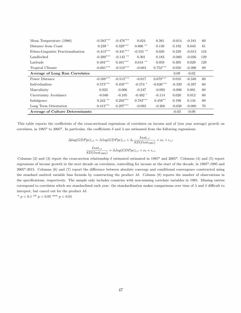
Mean Temperature (1986) -0.583∗∗∗ -0.476∗∗∗ 0.024 0.381 -0.014 -0.181 60
Distance from Coast 0.239 ∗ 0.329∗∗∗ 0.806 ∗∗ 0.130 0.192 0.043 61
Ethno-Linguistic Fractionalization -0.413∗∗∗ -0.441∗∗∗ -0.555 ∗∗ 0.029 0.229 -0.013 124
Landlocked -0.200∗∗∗ -0.142 ∗∗ 0.301 0.183 -0.060 -0.026 129
Latitude 0.494∗∗∗ 0.481∗∗∗ 0.618 ∗∗ 0.059 0.305 0.029 129
Tropical Climate -0.601∗∗∗ -0.518∗∗∗ -0.083 0.752∗∗∗ 0.050 -0.390 89
Average of Long Run Correlates 0.09 -0.02
Power Distance -0.588∗∗∗ -0.513∗∗∗ -0.017 0.679∗∗∗ 0.010 -0.348 60
Individualism 0.573∗∗∗ 0.459∗∗∗ -0.574 ∗ -0.626∗∗∗ -0.329 -0.287 60
Masculinity 0.023 -0.006 -0.247 -0.092 -0.006 0.001 60
Uncertainty Avoidance -0.040 -0.105 -0.492 ∗ -0.114 0.020 0.012 60
Indulgence 0.242 ∗∗ 0.292∗∗∗ 0.783∗∗∗ 0.458∗∗ 0.190 0.134 69
Long Term Orientation 0.412∗∗∗ 0.297∗∗∗ -0.092 -0.268 -0.038 -0.080 70
Average of Culture Determinants -0.03 -0.09
This table reports the coefficients of the cross-sectional regressions of correlates on income and of (ten year average) growth on
correlates, in 1985* to 2005*. In particular, the coefficients δ and λ are estimated from the following regressions:
∆log(GDPpc)i,t = βtlog(GDPpc)i,t + λtInsti,t
SD(Inst1985)+ αt + εi,t
Insti,tSD(Inst1985)
= δtlog(GDPpc)i,t + νt + εi,t
Columns (2) and (3) report the cross-section relationship δ estimated estimated in 1985* and 2005*. Columns (4) and (5) report
regressions of income growth in the next decade on correlates, controlling for income at the start of the decade, in 1985*-1995 and
2005*-2015. Columns (6) and (7) report the difference between absolute converge and conditional convergence constructed using
the standard omitted variable bias formula by constructing the product λδ. Column (8) reports the number of observations in
the specifications, respectively. The sample only includes countries with non-missing correlate variables in 1985. Missing entries
correspond to correlates which are standardized each year: the standardization makes comparisons over time of λ and δ difficult to
interpret, but cancel out for the product λδ.
* p < 0.1 ** p < 0.05 *** p < 0.01
47
Table 5: Absolute and conditional convergence in 1985 and 2005
Annual Growth in GDPpc (1985-1995) Annual Growth in GDPpc (2005-2015)
(1) (2) (3) (4) (5) (6) (7) (8)
Log GDP PC 0.420∗ -0.447 -0.435 -0.816 -0.794∗∗∗ -1.215∗∗∗ -0.791∗∗∗ -1.139∗∗∗
(0.252) (0.661) (0.457) (0.619) (0.154) (0.205) (0.233) (0.246)
Investment 0.298 -0.0469 0.384 0.416(0.377) (0.478) (0.319) (0.300)
Population growth -1.034 -1.024 -0.392∗∗∗ -0.415∗∗∗
(0.626) (0.661) (0.129) (0.148)
Barro-Lee Education 20-60 0.428 0.492 0.463∗ 0.535∗∗
(0.525) (0.619) (0.270) (0.267)
Polity 2 Score -0.558 -0.916 0.693∗ 0.0514(0.704) (0.728) (0.378) (0.400)
FH Political Rights 1.304 1.567∗ -0.193 0.378(0.989) (0.931) (0.464) (0.428)
Private Investment -0.184 -0.267 0.223 0.143(0.332) (0.329) (0.394) (0.344)
Government Spending -0.0168 0.0773 -0.551∗∗ -0.764∗∗∗
(0.386) (0.415) (0.275) (0.256)
Inflation -0.0994 -0.0284 -1.438∗ -1.273∗
(0.235) (0.243) (0.772) (0.722)
FH Civil Liberties 0.0958 -0.481 -0.0784 -0.333(0.647) (0.749) (0.782) (0.724)
Credit to Private Sector 0.915∗ 0.875 0.483 0.494∗
(0.467) (0.531) (0.313) (0.291)
Credit by Financial Sector -0.394 -0.546 -0.733∗ -0.798∗∗
(0.507) (0.573) (0.376) (0.368)
Constant -2.172 5.546 1.213 6.644 9.387∗∗∗ 11.42∗∗∗ 10.90∗∗∗ 12.31∗∗∗
(2.230) (5.458) (3.313) (4.687) (1.471) (1.732) (2.277) (2.306)
Observations 73 73 73 73 113 113 113 113R-Squared 0.0283 0.155 0.152 0.228 0.214 0.333 0.306 0.417
Standard errors in parentheses∗ p < 0.1, ∗∗ p < 0.05, ∗∗∗ p < 0.01
Notes: This table reports absolute and conditional convergence regressions, for 1985*-1995 and 2005*-2015, for the fullest list ofSolow and short-run correlates which allow a reasonable sample size of 72 in 1985. The covariates include Investment, Populationgrowth, Barro-lee education attainment, polity2 score, Freedom House political rights, Freedom House civil liberty, privateinvestment ratio, government spending, inflation, credit provided to private sector, credit by financial sector, and education gendergap. Columns (1-4) report regressions for 1985-1995, and columns (5-8) for 2005-2015. Column (1) is the absolute convergenceregression. Column (2) conditions on the enhanced Solow fundamentals - the fundamental determinants of steady state income inthe Solow model. Column (3) conditions on other policies and institutions and column (4) conditions on both. Robust standarderrors are reported in parentheses. * p < 0.1, ** p < 0.05, *** p < 0.01
48
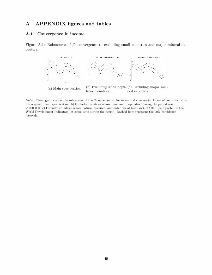
A APPENDIX figures and tables
A.1 Convergence in income
Figure A.1: Robustness of β−convergence to excluding small countries and major mineral ex-porters.
(a) Main specification. (b) Excluding small popu-lation countries.
(c) Excluding major min-eral exporters.
Notes: These graphs show the robustness of the β-convergence plot to natural changes in the set of countries. a) isthe original, main specification. b) Excludes countries whose maximum population during the period was< 200, 000. c) Excludes countries whose natural resources accounted for at least 75% of GDP (as reported in theWorld Development Indicators) at some time during the period. Dashed lines represent the 90% confidenceintervals.
49
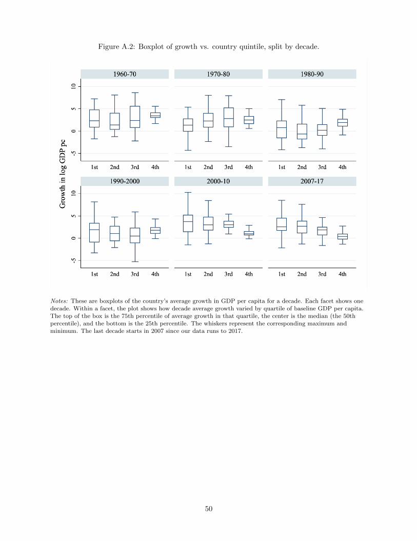
Figure A.2: Boxplot of growth vs. country quintile, split by decade.
Notes: These are boxplots of the country’s average growth in GDP per capita for a decade. Each facet shows onedecade. Within a facet, the plot shows how decade average growth varied by quartile of baseline GDP per capita.The top of the box is the 75th percentile of average growth in that quartile, the center is the median (the 50thpercentile), and the bottom is the 25th percentile. The whiskers represent the corresponding maximum andminimum. The last decade starts in 2007 since our data runs to 2017.
50
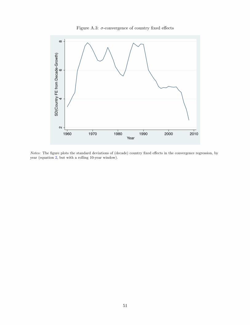
Figure A.3: σ-convergence of country fixed effects
24
68
SD(C
ount
ry F
E fro
m D
ecad
e-G
row
th)
1960 1970 1980 1990 2000 2010Year
Notes: The figure plots the standard deviations of (decade) country fixed effects in the convergence regression, byyear (equation 2, but with a rolling 10-year window).
51
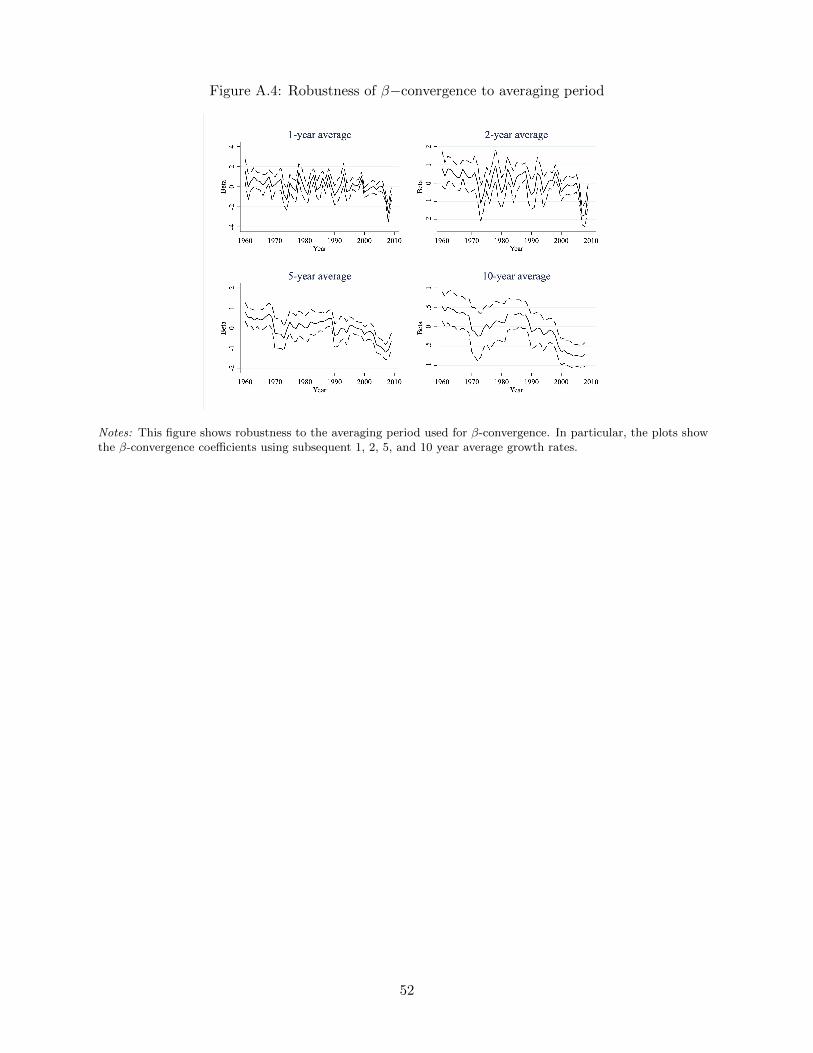
Figure A.4: Robustness of β−convergence to averaging period
Notes: This figure shows robustness to the averaging period used for β-convergence. In particular, the plots showthe β-convergence coefficients using subsequent 1, 2, 5, and 10 year average growth rates.
52
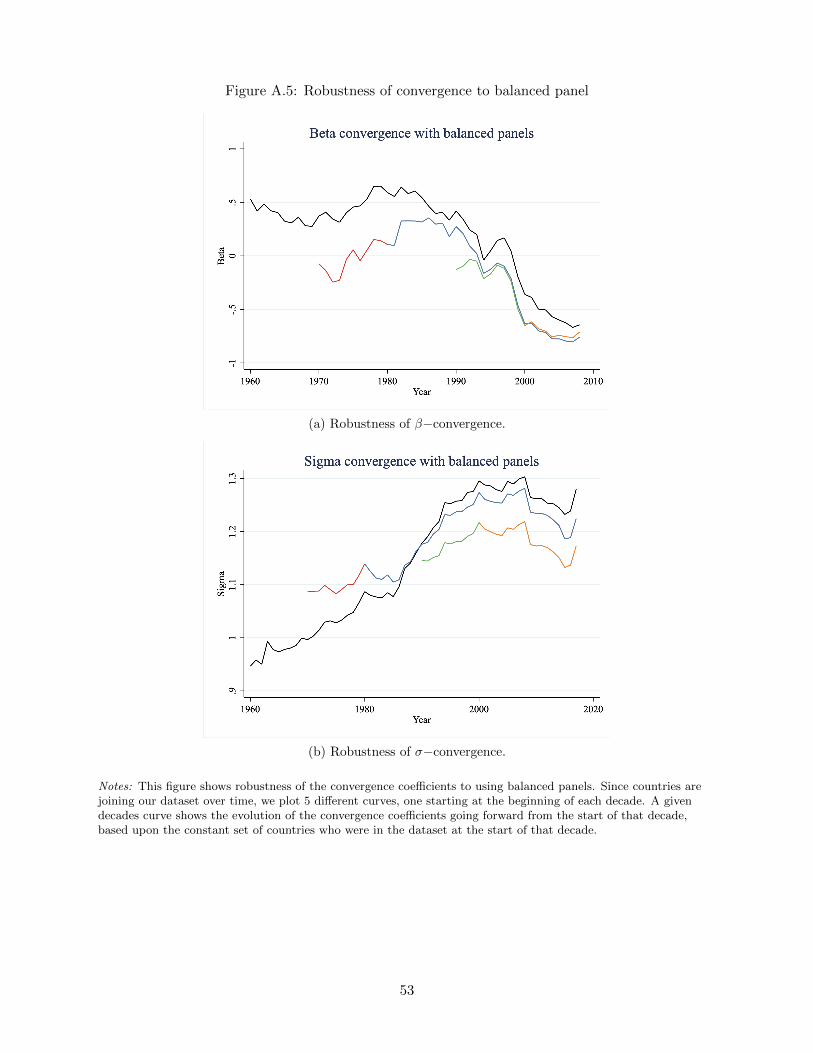
Figure A.5: Robustness of convergence to balanced panel
(a) Robustness of β−convergence.
(b) Robustness of σ−convergence.
Notes: This figure shows robustness of the convergence coefficients to using balanced panels. Since countries arejoining our dataset over time, we plot 5 different curves, one starting at the beginning of each decade. A givendecades curve shows the evolution of the convergence coefficients going forward from the start of that decade,based upon the constant set of countries who were in the dataset at the start of that decade.
53
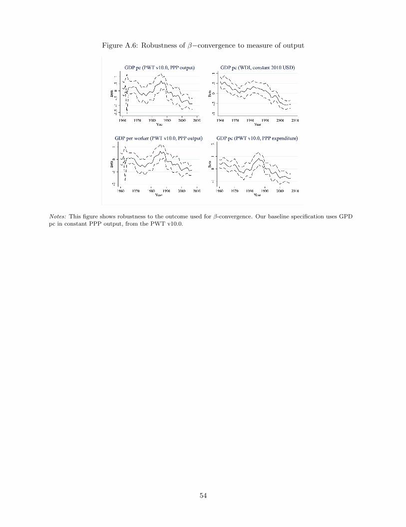
Figure A.6: Robustness of β−convergence to measure of output
Notes: This figure shows robustness to the outcome used for β-convergence. Our baseline specification uses GPDpc in constant PPP output, from the PWT v10.0.
54
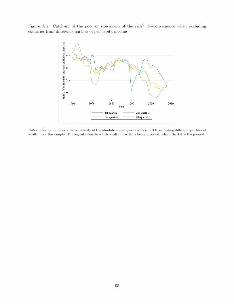
Figure A.7: Catch-up of the poor or slow-down of the rich? β−convergence when excludingcountries from different quartiles of per capita income
Notes: This figure reports the sensitivity of the absolute convergence coefficient β to excluding different quartiles ofwealth from the sample. The legend refers to which wealth quartile is being dropped, where the 1st is the poorest.
55
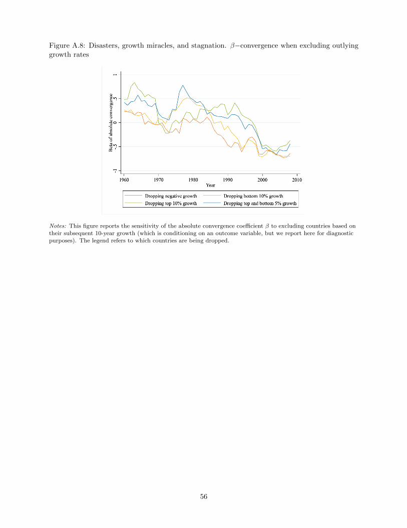
Figure A.8: Disasters, growth miracles, and stagnation. β−convergence when excluding outlyinggrowth rates
Notes: This figure reports the sensitivity of the absolute convergence coefficient β to excluding countries based ontheir subsequent 10-year growth (which is conditioning on an outcome variable, but we report here for diagnosticpurposes). The legend refers to which countries are being dropped.
56
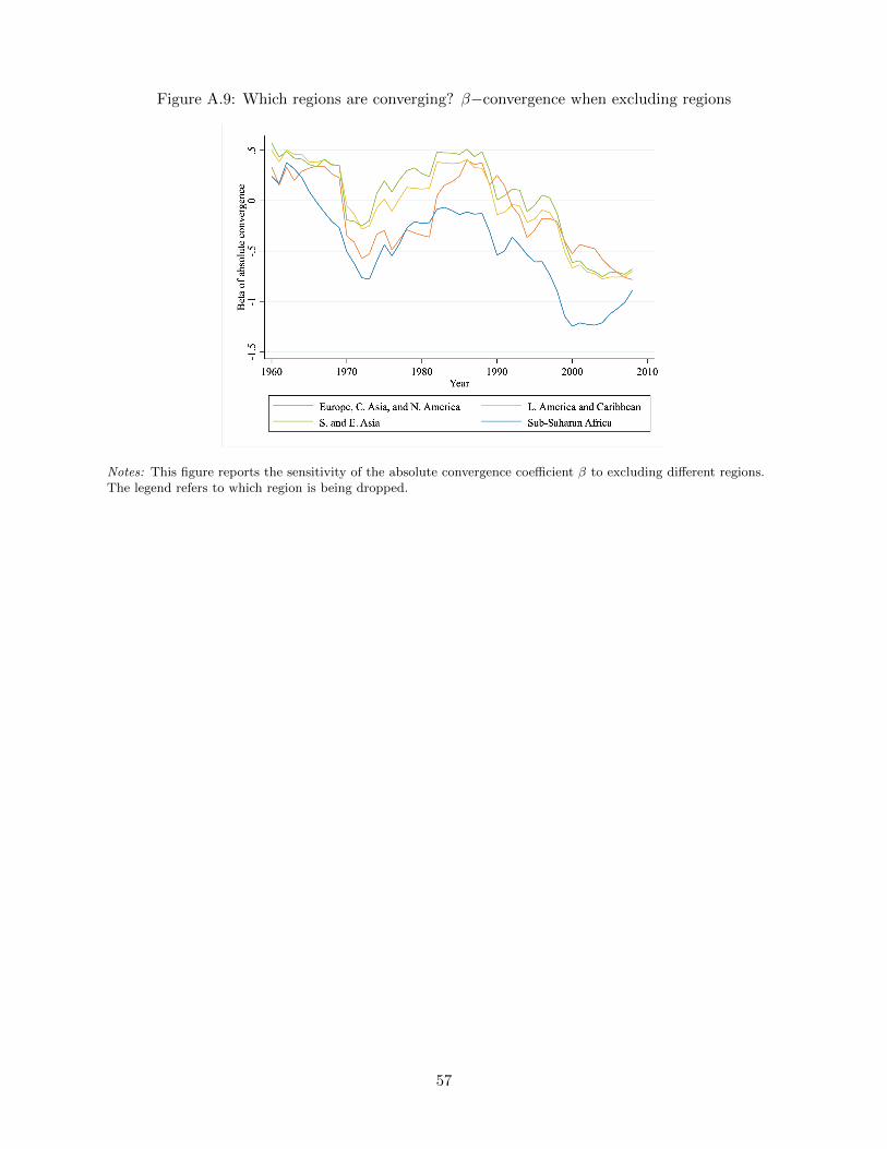
Figure A.9: Which regions are converging? β−convergence when excluding regions
Notes: This figure reports the sensitivity of the absolute convergence coefficient β to excluding different regions.The legend refers to which region is being dropped.
57
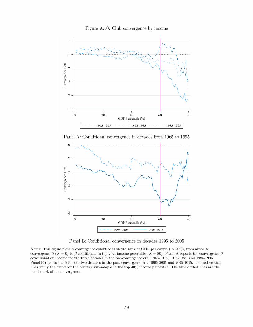
Figure A.10: Club convergence by income
-4-3
-2-1
01
Con
verg
ence
Bet
a
0 20 40 60 80GDP Percentile (%)
1965-1975 1975-1985 1985-1995
Panel A: Conditional convergence in decades from 1965 to 1995
-2.5
-2-1
.5-1
-.50
Con
verg
ence
Bet
a
0 20 40 60 80GDP Percentile (%)
1995-2005 2005-2015
Panel B: Conditional convergence in decades 1995 to 2005
Notes: This figure plots β convergence conditional on the rank of GDP per capita ( > X%), from absoluteconvergence β (X = 0) to β conditional in top 20% income percentile (X = 80). Panel A reports the convergence βconditional on income for the three decades in the pre-convergence era: 1965-1975, 1975-1985, and 1985-1995.Panel B reports the β for the two decades in the post-convergence era: 1995-2005 and 2005-2015. The red verticallines imply the cutoff for the country sub-sample in the top 40% income percentile. The blue dotted lines are thebenchmark of no convergence.
58
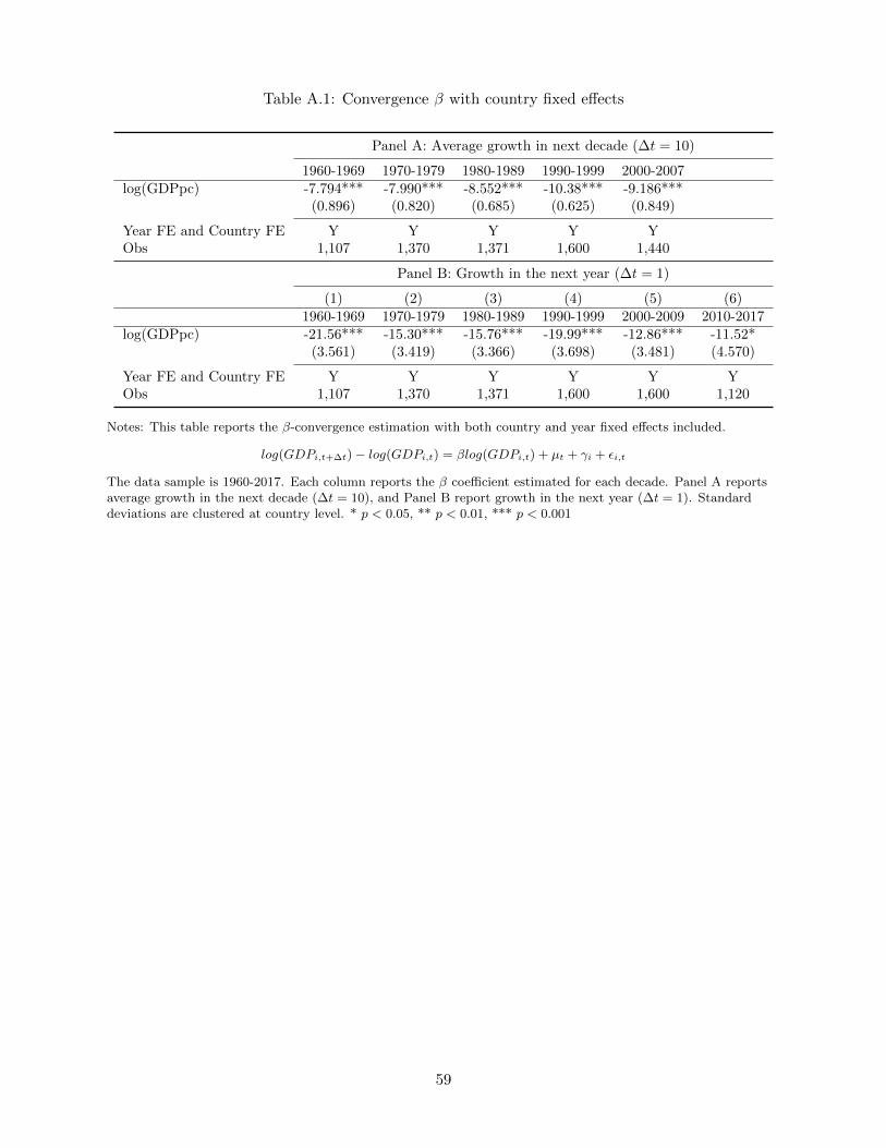
Table A.1: Convergence β with country fixed effects
Panel A: Average growth in next decade (∆t = 10)
1960-1969 1970-1979 1980-1989 1990-1999 2000-2007log(GDPpc) -7.794*** -7.990*** -8.552*** -10.38*** -9.186***
(0.896) (0.820) (0.685) (0.625) (0.849)
Year FE and Country FE Y Y Y Y YObs 1,107 1,370 1,371 1,600 1,440
Panel B: Growth in the next year (∆t = 1)
(1) (2) (3) (4) (5) (6)1960-1969 1970-1979 1980-1989 1990-1999 2000-2009 2010-2017
log(GDPpc) -21.56*** -15.30*** -15.76*** -19.99*** -12.86*** -11.52*(3.561) (3.419) (3.366) (3.698) (3.481) (4.570)
Year FE and Country FE Y Y Y Y Y YObs 1,107 1,370 1,371 1,600 1,600 1,120
Notes: This table reports the β-convergence estimation with both country and year fixed effects included.
log(GDPi,t+∆t) − log(GDPi,t) = βlog(GDPi,t) + µt + γi + εi,t
The data sample is 1960-2017. Each column reports the β coefficient estimated for each decade. Panel A reportsaverage growth in the next decade (∆t = 10), and Panel B report growth in the next year (∆t = 1). Standarddeviations are clustered at country level. * p < 0.05, ** p < 0.01, *** p < 0.001
59
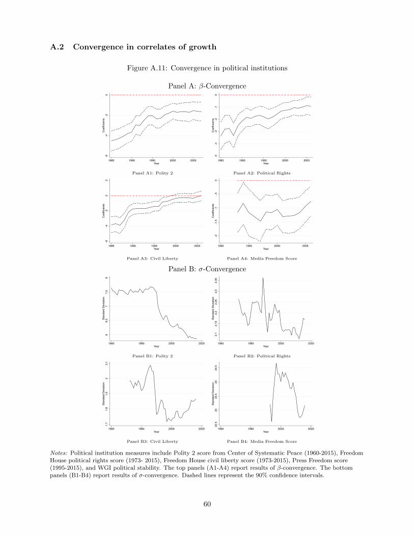
A.2 Convergence in correlates of growth
Figure A.11: Convergence in political institutions
Panel A: β-Convergence
-6-4
-20
Coefficients
1985 1990 1995 2000 2005Year
Panel A1: Polity 2
-5-4
-3-2
-10
Coefficients
1985 1990 1995 2000 2005Year
Panel A2: Political Rights
-6-4
-20
2Coefficients
1985 1990 1995 2000 2005Year
Panel A3: Civil Liberty
-2-1.5
-1-.5
0Coefficients
1990 1995 2000 2005Year
Panel A4: Media Freedom Score
Panel B: σ-Convergence
66.
57
7.5
8St
anda
rd D
evia
tion
1960 1980 2000 2020Year
Panel B1: Polity 2
2.1
2.15
2.2
2.25
2.3
2.35
Stan
dard
Dev
iatio
n
1960 1980 2000 2020Year
Panel B2: Political Rights
1.7
1.8
1.9
22.
1St
anda
rd D
evia
tion
1960 1980 2000 2020Year
Panel B3: Civil Liberty
22.5
2323
.524
24.5
Stan
dard
Dev
iatio
n
1960 1980 2000 2020Year
Panel B4: Media Freedom Score
Notes: Political institution measures include Polity 2 score from Center of Systematic Peace (1960-2015), FreedomHouse political rights score (1973- 2015), Freedom House civil liberty score (1973-2015), Press Freedom score(1995-2015), and WGI political stability. The top panels (A1-A4) report results of β-convergence. The bottompanels (B1-B4) report results of σ-convergence. Dashed lines represent the 90% confidence intervals.
60
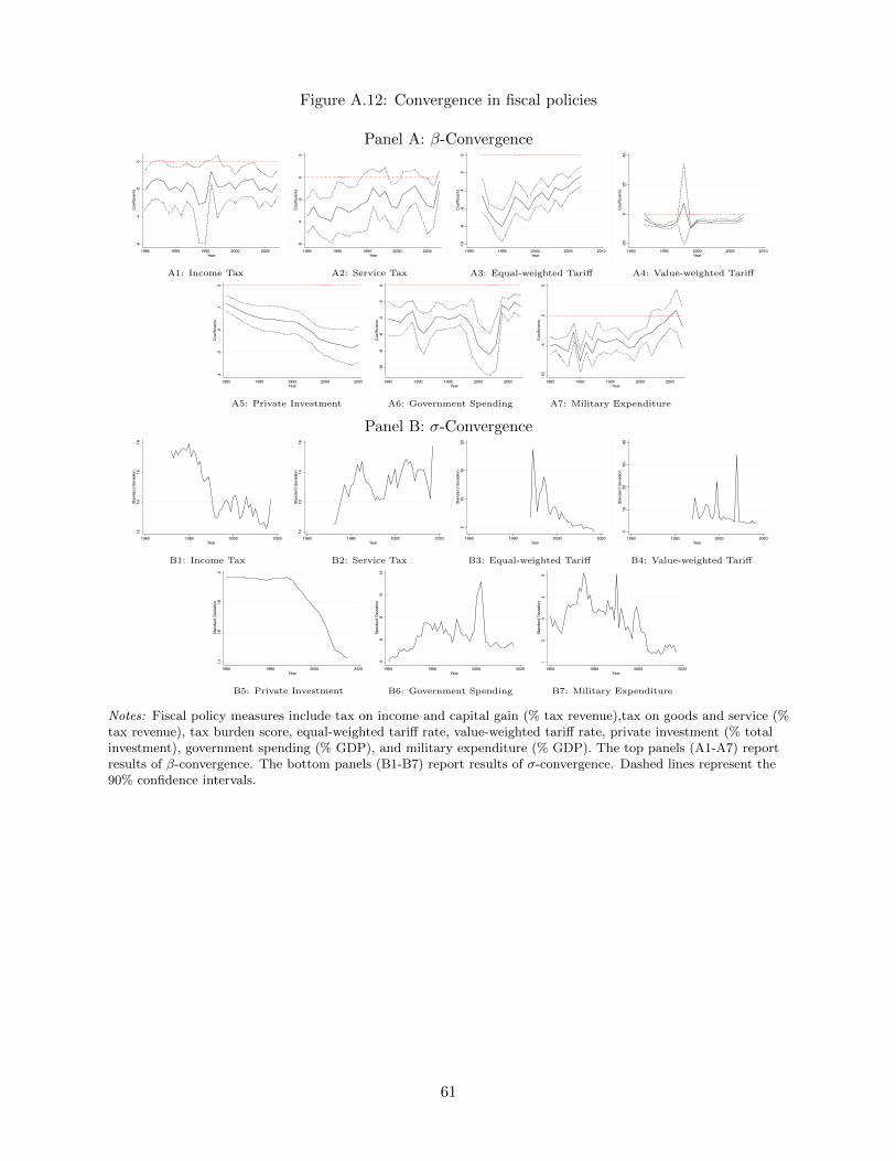
Figure A.12: Convergence in fiscal policies
Panel A: β-Convergence-6
-4-2
0Coefficients
1985 1990 1995 2000 2005Year
A1: Income Tax
-6-4
-20
2Coefficients
1985 1990 1995 2000 2005Year
A2: Service Tax
-10
-8-6
-4-2
0Coefficients
1990 1995 2000 2005 2010Year
A3: Equal-weighted Tariff
-20
020
40Coefficients
1990 1995 2000 2005 2010Year
A4: Value-weighted Tariff
-4-3
-2-1
0Coefficients
1985 1990 1995 2000 2005Year
A5: Private Investment
-10
-8-6
-4-2
0Coefficients
1985 1990 1995 2000 2005Year
A6: Government Spending
-10
-50
5Coefficients
1985 1990 1995 2000 2005Year
A7: Military Expenditure
Panel B: σ-Convergence
1214
1618
Stan
dard
Dev
iatio
n
1960 1980 2000 2020Year
B1: Income Tax
1012
1416
Stan
dard
Dev
iatio
n
1960 1980 2000 2020Year
B2: Service Tax
510
1520
Stan
dard
Dev
iatio
n
1960 1980 2000 2020Year
B3: Equal-weighted Tariff
010
2030
40St
anda
rd D
evia
tion
1960 1980 2000 2020Year
B4: Value-weighted Tariff
.14
.16
.18
.2St
anda
rd D
evia
tion
1960 1980 2000 2020Year
B5: Private Investment
46
810
12St
anda
rd D
evia
tion
1960 1980 2000 2020Year
B6: Government Spending
12
34
5St
anda
rd D
evia
tion
1960 1980 2000 2020Year
B7: Military Expenditure
Notes: Fiscal policy measures include tax on income and capital gain (% tax revenue),tax on goods and service (%tax revenue), tax burden score, equal-weighted tariff rate, value-weighted tariff rate, private investment (% totalinvestment), government spending (% GDP), and military expenditure (% GDP). The top panels (A1-A7) reportresults of β-convergence. The bottom panels (B1-B7) report results of σ-convergence. Dashed lines represent the90% confidence intervals.
61
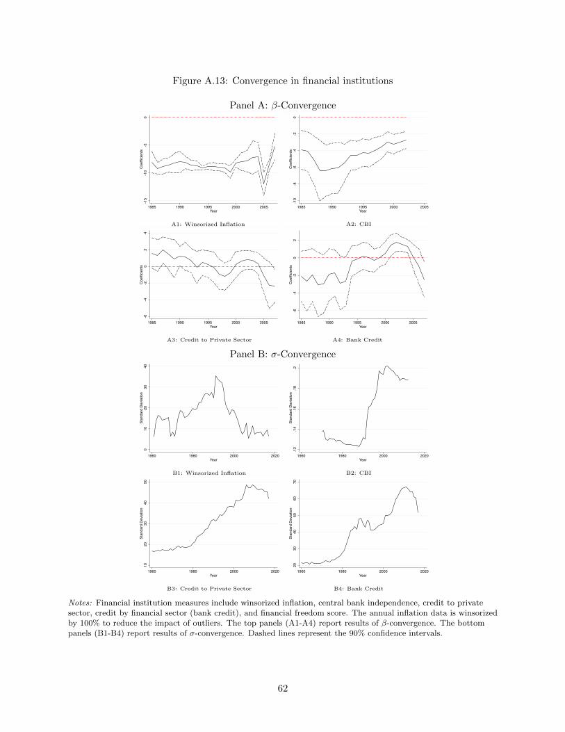
Figure A.13: Convergence in financial institutions
Panel A: β-Convergence
-15
-10
-50
Coefficients
1985 1990 1995 2000 2005Year
A1: Winsorized Inflation
-10
-8-6
-4-2
0Coefficients
1985 1990 1995 2000 2005Year
A2: CBI
-6-4
-20
24
Coefficients
1985 1990 1995 2000 2005Year
A3: Credit to Private Sector
-6-4
-20
2Coefficients
1985 1990 1995 2000 2005Year
A4: Bank Credit
Panel B: σ-Convergence
010
2030
40St
anda
rd D
evia
tion
1960 1980 2000 2020Year
B1: Winsorized Inflation
.12
.14
.16
.18
.2St
anda
rd D
evia
tion
1960 1980 2000 2020Year
B2: CBI
1020
3040
50St
anda
rd D
evia
tion
1960 1980 2000 2020Year
B3: Credit to Private Sector
2030
4050
6070
Stan
dard
Dev
iatio
n
1960 1980 2000 2020Year
B4: Bank Credit
Notes: Financial institution measures include winsorized inflation, central bank independence, credit to privatesector, credit by financial sector (bank credit), and financial freedom score. The annual inflation data is winsorizedby 100% to reduce the impact of outliers. The top panels (A1-A4) report results of β-convergence. The bottompanels (B1-B4) report results of σ-convergence. Dashed lines represent the 90% confidence intervals.
62
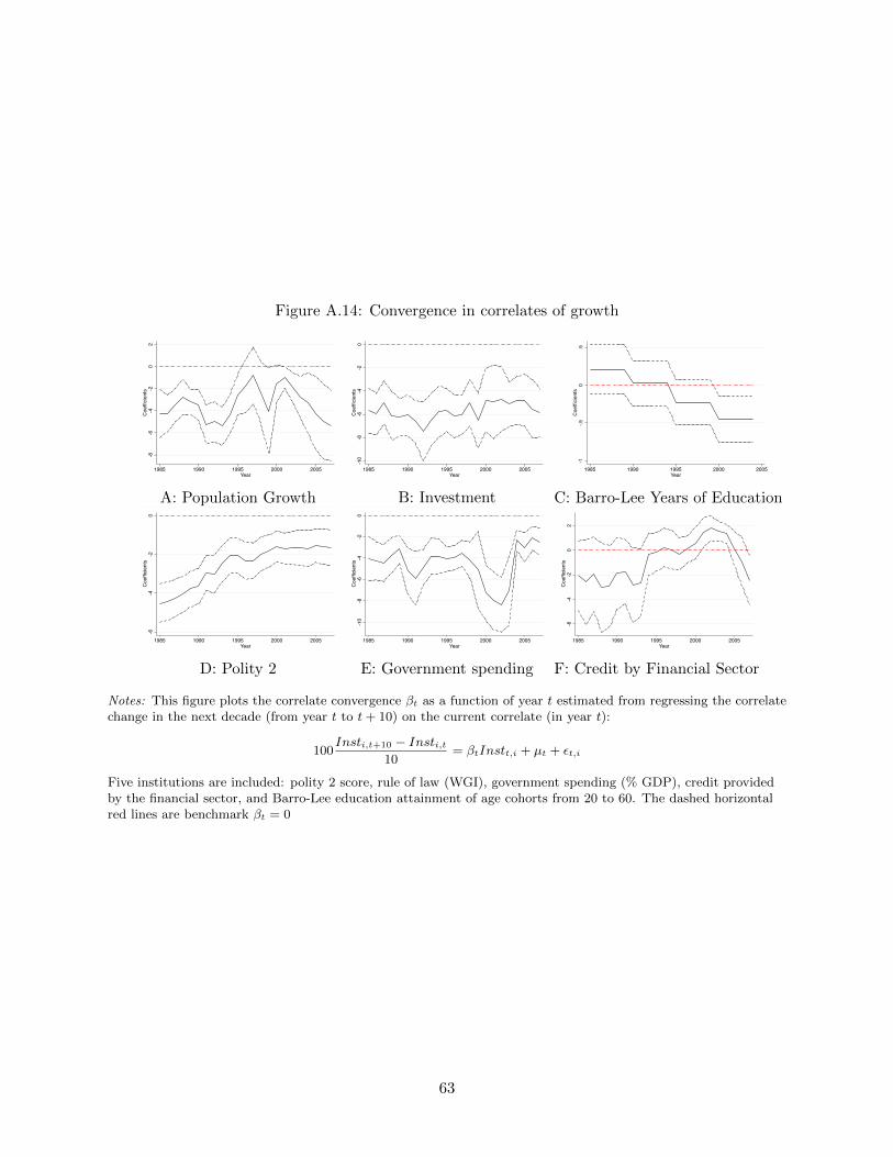
Figure A.14: Convergence in correlates of growth
-8-6
-4-2
02
Coefficients
1985 1990 1995 2000 2005Year
A: Population Growth
-10
-8-6
-4-2
0Coefficients
1985 1990 1995 2000 2005Year
B: Investment
-1-.5
0.5
Coefficients
1985 1990 1995 2000 2005Year
C: Barro-Lee Years of Education
-6-4
-20
Coefficients
1985 1990 1995 2000 2005Year
D: Polity 2
-10
-8-6
-4-2
0Coefficients
1985 1990 1995 2000 2005Year
E: Government spending
-6-4
-20
2Coefficients
1985 1990 1995 2000 2005Year
F: Credit by Financial Sector
Notes: This figure plots the correlate convergence βt as a function of year t estimated from regressing the correlatechange in the next decade (from year t to t+ 10) on the current correlate (in year t):
100Insti,t+10 − Insti,t
10= βtInstt,i + µt + εt,i
Five institutions are included: polity 2 score, rule of law (WGI), government spending (% GDP), credit providedby the financial sector, and Barro-Lee education attainment of age cohorts from 20 to 60. The dashed horizontalred lines are benchmark βt = 0
63
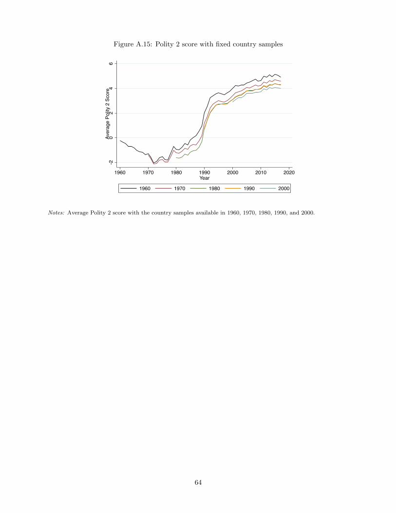
Figure A.15: Polity 2 score with fixed country samples
-20
24
6Av
erag
e Po
lity
2 Sc
ore
1960 1970 1980 1990 2000 2010 2020Year
1960 1970 1980 1990 2000
Notes: Average Polity 2 score with the country samples available in 1960, 1970, 1980, 1990, and 2000.
64
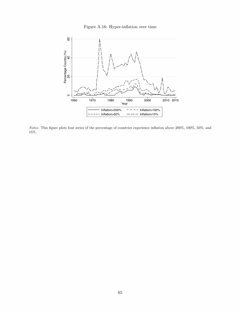
Figure A.16: Hyper-inflation over time
020
4060
Perc
enta
ge C
ount
ry (%
)
1960 1970 1980 1990 2000 2010 2015Year
Inflation>200% Inflation>100%Inflation>50% Inflation>15%
Notes: This figure plots four series of the percentage of countries experience inflation above 200%, 100%, 50%, and15%.
65
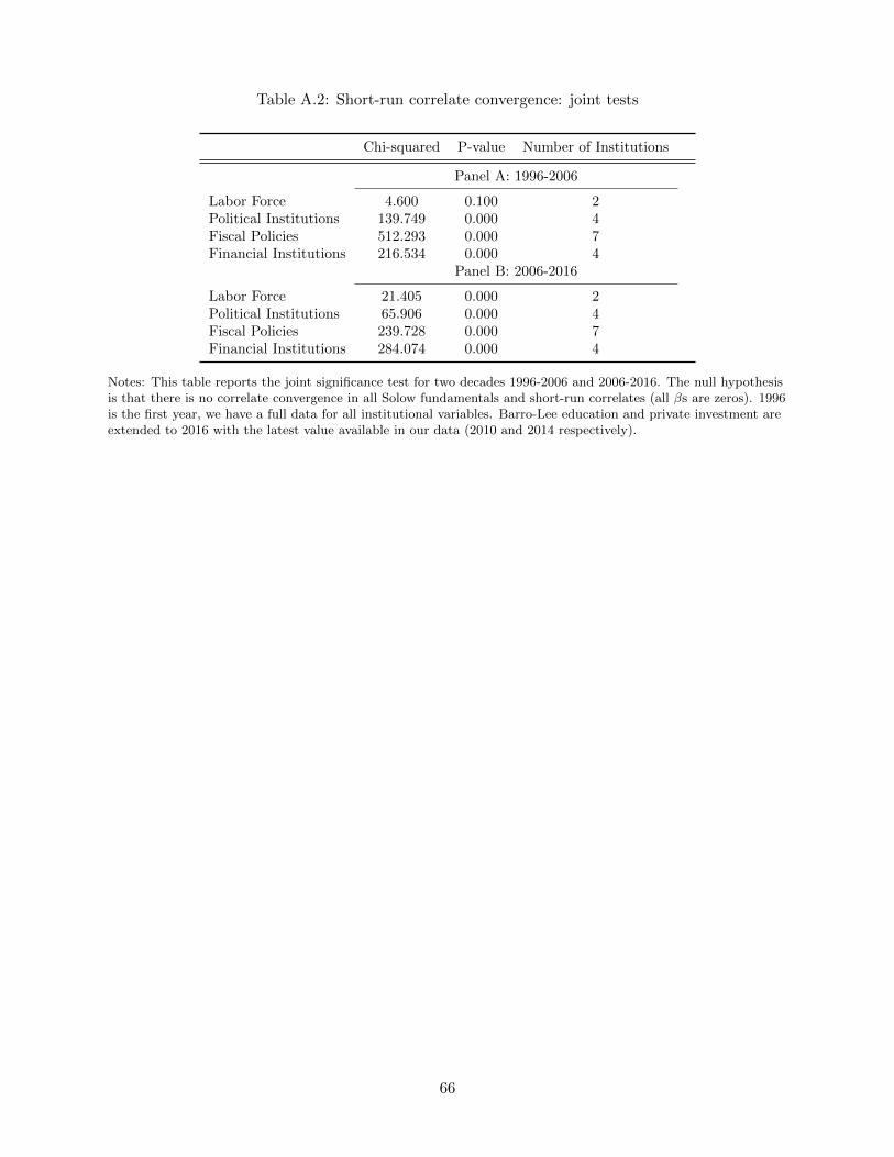
Table A.2: Short-run correlate convergence: joint tests
Chi-squared P-value Number of Institutions
Panel A: 1996-2006
Labor Force 4.600 0.100 2Political Institutions 139.749 0.000 4Fiscal Policies 512.293 0.000 7Financial Institutions 216.534 0.000 4
Panel B: 2006-2016
Labor Force 21.405 0.000 2Political Institutions 65.906 0.000 4Fiscal Policies 239.728 0.000 7Financial Institutions 284.074 0.000 4
Notes: This table reports the joint significance test for two decades 1996-2006 and 2006-2016. The null hypothesisis that there is no correlate convergence in all Solow fundamentals and short-run correlates (all βs are zeros). 1996is the first year, we have a full data for all institutional variables. Barro-Lee education and private investment areextended to 2016 with the latest value available in our data (2010 and 2014 respectively).
66
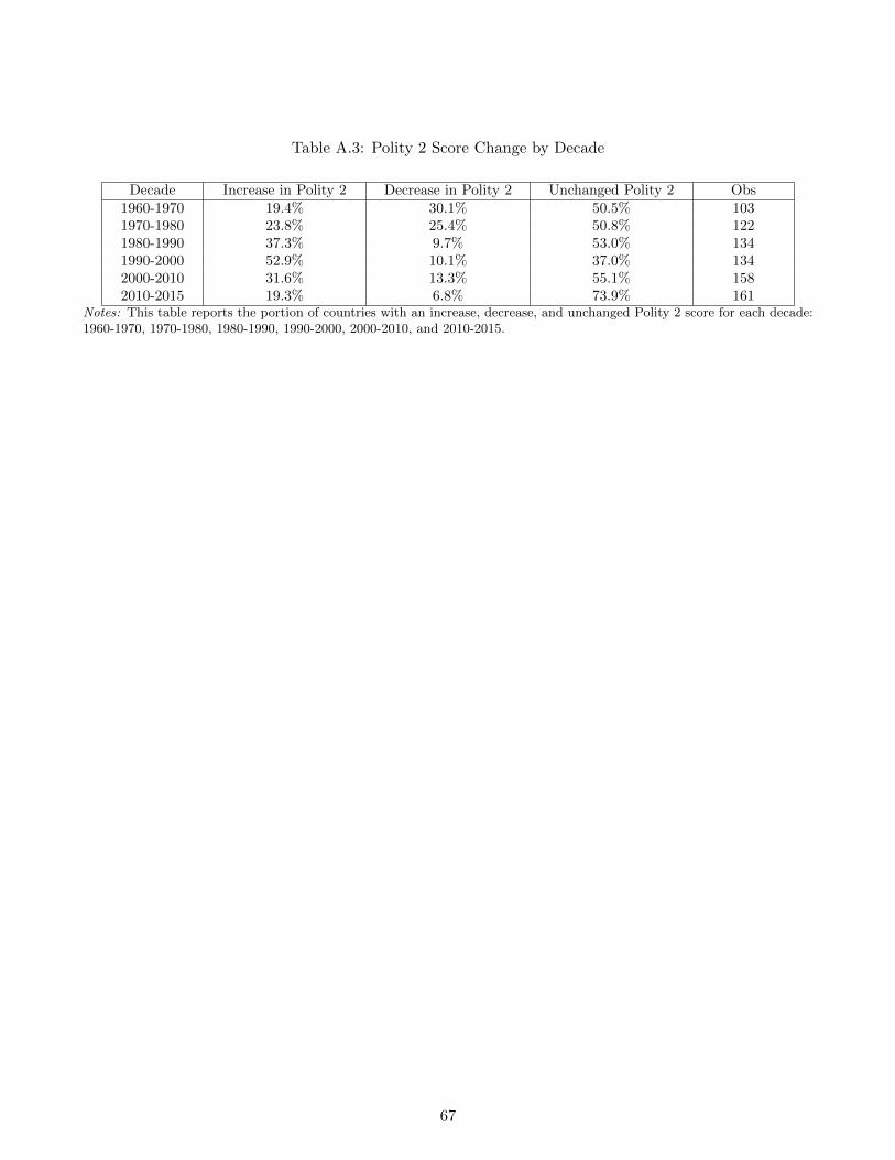
Table A.3: Polity 2 Score Change by Decade
Decade Increase in Polity 2 Decrease in Polity 2 Unchanged Polity 2 Obs1960-1970 19.4% 30.1% 50.5% 1031970-1980 23.8% 25.4% 50.8% 1221980-1990 37.3% 9.7% 53.0% 1341990-2000 52.9% 10.1% 37.0% 1342000-2010 31.6% 13.3% 55.1% 1582010-2015 19.3% 6.8% 73.9% 161
Notes: This table reports the portion of countries with an increase, decrease, and unchanged Polity 2 score for each decade:1960-1970, 1970-1980, 1980-1990, 1990-2000, 2000-2010, and 2010-2015.
67
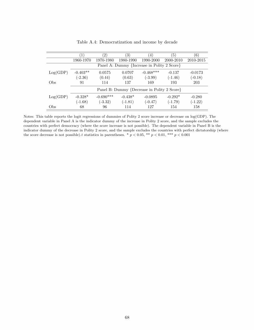
Table A.4: Democratization and income by decade
(1) (2) (3) (4) (5) (6)1960-1970 1970-1980 1980-1990 1990-2000 2000-2010 2010-2015
Panel A: Dummy {Increase in Polity 2 Score}
Log(GDP) -0.403** 0.0575 0.0707 -0.468*** -0.137 -0.0173(-2.36) (0.44) (0.63) (-3.99) (-1.46) (-0.18)
Obs 91 114 137 169 193 203
Panel B: Dummy {Decrease in Polity 2 Score}
Log(GDP) -0.328* -0.690*** -0.438* -0.0895 -0.292* -0.280(-1.68) (-3.32) (-1.81) (-0.47) (-1.79) (-1.22)
Obs 68 96 114 127 154 158
Notes: This table reports the logit regressions of dummies of Polity 2 score increase or decrease on log(GDP). Thedependent variable in Panel A is the indicator dummy of the increase in Polity 2 score, and the sample excludes thecountries with perfect democracy (where the score increase is not possible). The dependent variable in Panel B is theindicator dummy of the decrease in Polity 2 score, and the sample excludes the countries with perfect dictatorship (wherethe score decrease is not possible).t statistics in parentheses. * p < 0.05, ** p < 0.01, *** p < 0.001
68
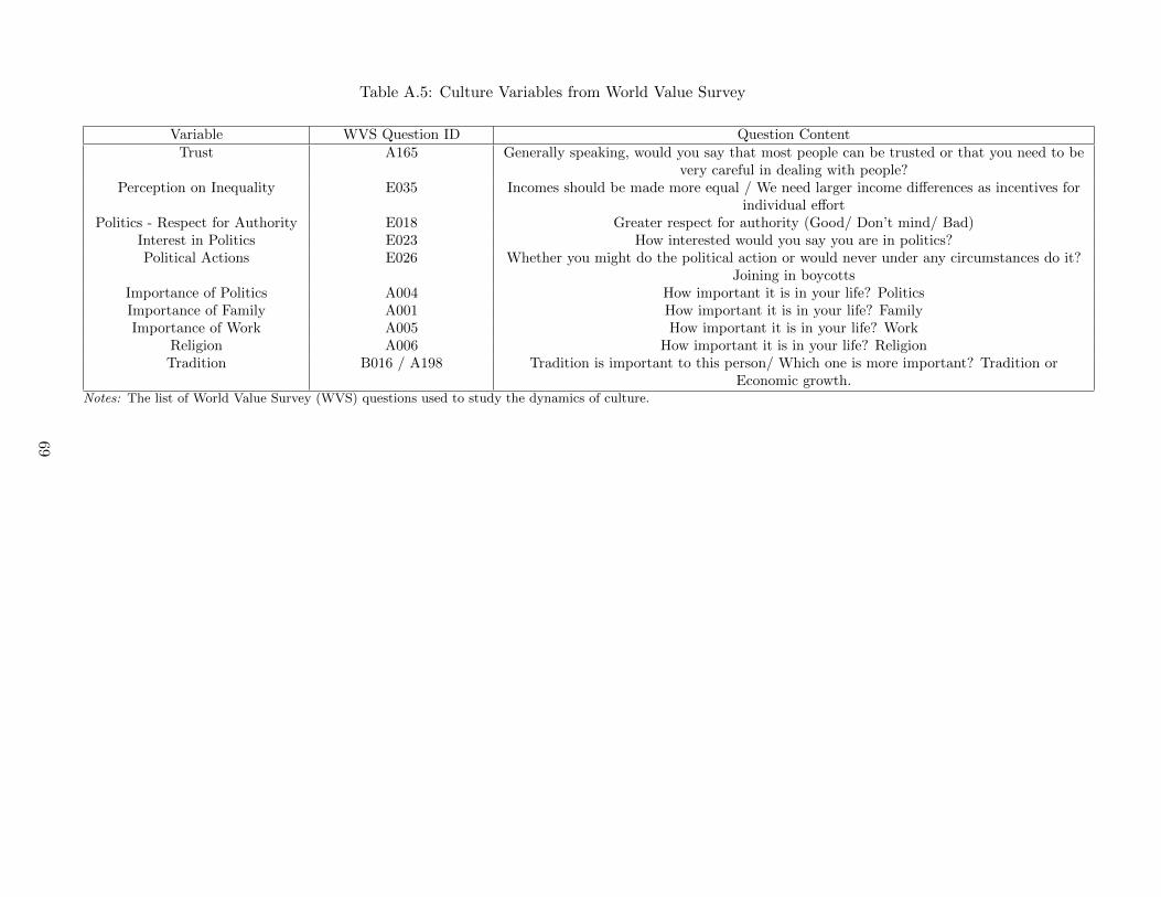
Table A.5: Culture Variables from World Value Survey
Variable WVS Question ID Question ContentTrust A165 Generally speaking, would you say that most people can be trusted or that you need to be
very careful in dealing with people?Perception on Inequality E035 Incomes should be made more equal / We need larger income differences as incentives for
individual effortPolitics - Respect for Authority E018 Greater respect for authority (Good/ Don’t mind/ Bad)
Interest in Politics E023 How interested would you say you are in politics?Political Actions E026 Whether you might do the political action or would never under any circumstances do it?
Joining in boycottsImportance of Politics A004 How important it is in your life? PoliticsImportance of Family A001 How important it is in your life? FamilyImportance of Work A005 How important it is in your life? Work
Religion A006 How important it is in your life? ReligionTradition B016 / A198 Tradition is important to this person/ Which one is more important? Tradition or
Economic growth.Notes: The list of World Value Survey (WVS) questions used to study the dynamics of culture.
69
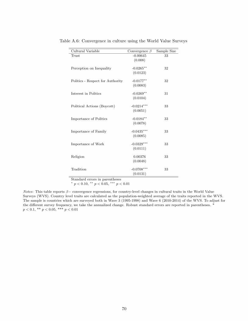
Table A.6: Convergence in culture using the World Value Surveys
Cultural Variable Convergence β Sample Size
Trust -0.00645 33(0.008)
Perception on Inequality -0.0265∗∗ 32(0.0123)
Politics - Respect for Authority -0.0177∗∗ 32(0.0083)
Interest in Politics -0.0269∗∗ 31(0.0104)
Political Actions (Boycott) -0.0214∗∗∗ 33(0.0051)
Importance of Politics -0.0184∗∗ 33(0.0078)
Importance of Family -0.0435∗∗∗ 33(0.0085)
Importance of Work -0.0329∗∗∗ 33(0.0111)
Religion 0.00376 33(0.0048)
Tradition -0.0708∗∗∗ 33(0.0131)
Standard errors in parentheses∗ p < 0.10, ∗∗ p < 0.05, ∗∗∗ p < 0.01
Notes: This table reports β− convergence regressions, for country-level changes in cultural traits in the World ValueSurveys (WVS). Country level traits are calculated as the population-weighted average of the traits reported in the WVS.The sample is countries which are surveyed both in Wave 3 (1995-1998) and Wave 6 (2010-2014) of the WVS. To adjust forthe different survey frequency, we take the annualized change. Robust standard errors are reported in parentheses. *p < 0.1, ** p < 0.05, *** p < 0.01
70
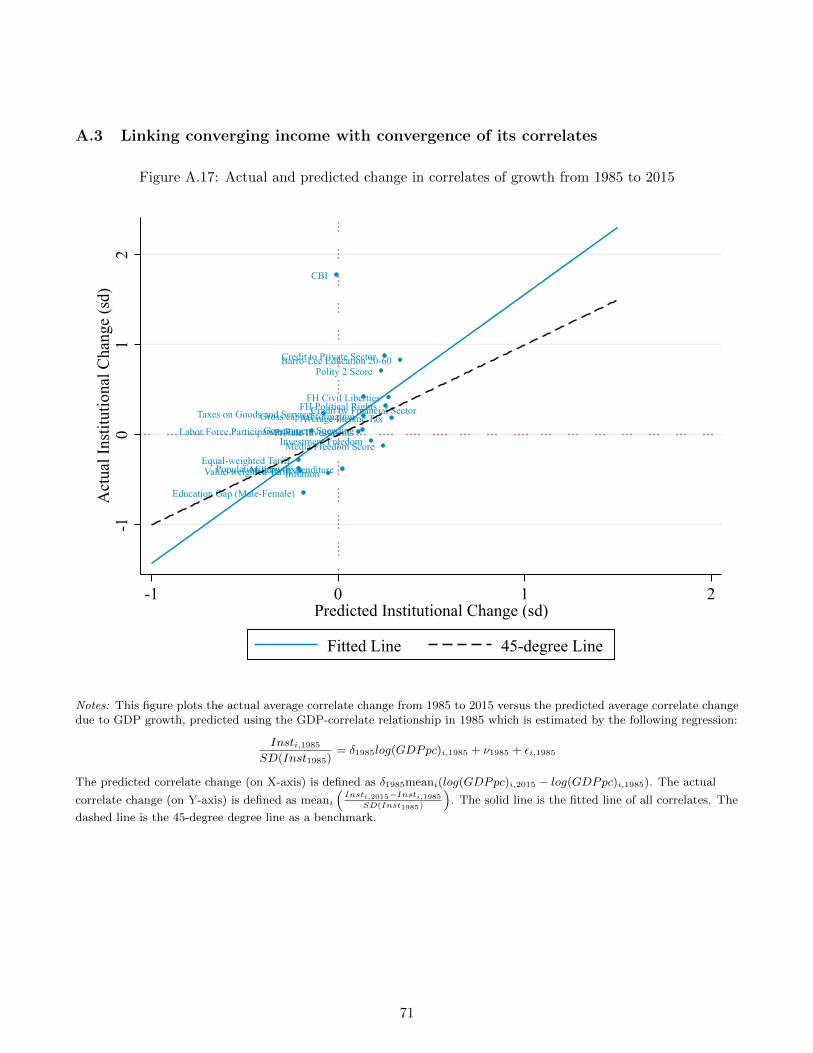
A.3 Linking converging income with convergence of its correlates
Figure A.17: Actual and predicted change in correlates of growth from 1985 to 2015
Gross capital formation
Population growth
Barro-Lee Education 20-60
Education Gap (Male-Female)
Labor Force Participation Rate
Polity 2 Score
FH Political RightsFH Civil Liberties
Media Freedom ScoreEqual-weighted TariffValue-weighted Tariff
Average Income TaxTaxes on Goods and Services
Government SpendingPrivate Investment
Military ExpenditureInflation
CBI
Credit to Private Sector
Credit by Financial Sector
Investment Freedom
-10
12
Act
ual I
nstit
utio
nal C
hang
e (s
d)
-1 0 1 2Predicted Institutional Change (sd)
Fitted Line 45-degree Line
Notes: This figure plots the actual average correlate change from 1985 to 2015 versus the predicted average correlate changedue to GDP growth, predicted using the GDP-correlate relationship in 1985 which is estimated by the following regression:
Insti,1985
SD(Inst1985)= δ1985log(GDPpc)i,1985 + ν1985 + εi,1985
The predicted correlate change (on X-axis) is defined as δ1985meani(log(GDPpc)i,2015 − log(GDPpc)i,1985). The actual
correlate change (on Y-axis) is defined as meani
(Insti,2015−Insti,1985
SD(Inst1985)
). The solid line is the fitted line of all correlates. The
dashed line is the 45-degree degree line as a benchmark.
71
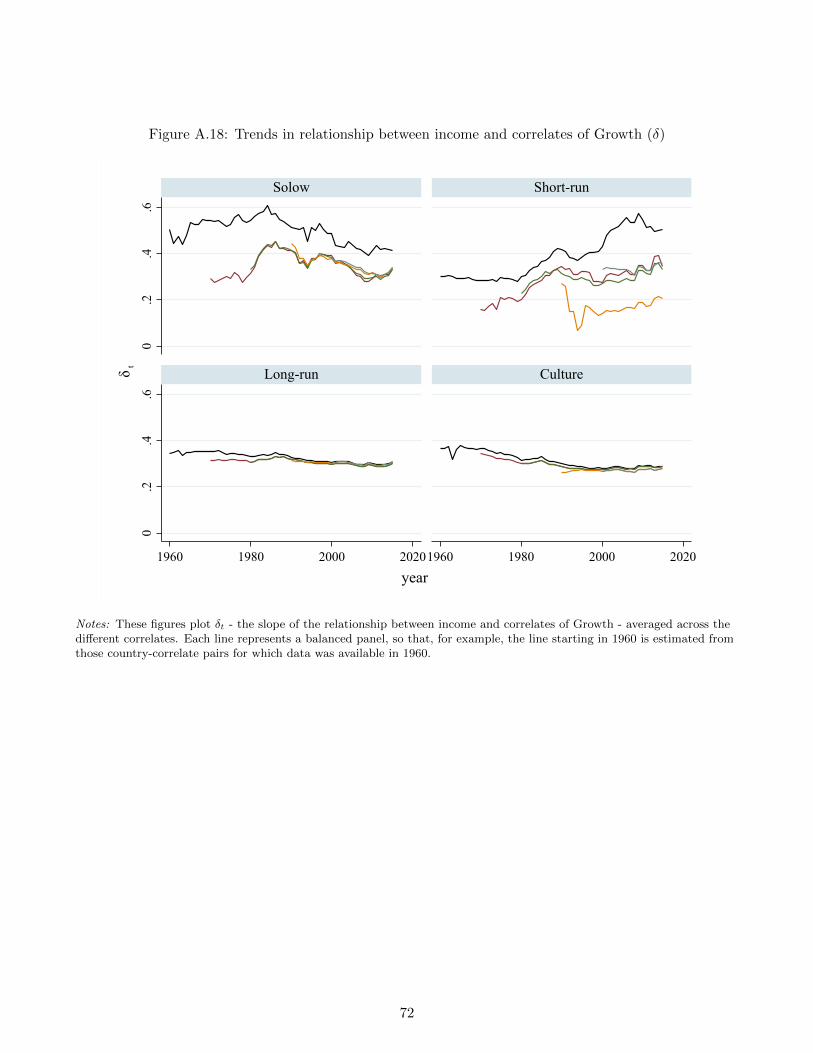
Figure A.18: Trends in relationship between income and correlates of Growth (δ)0
.2.4
.60
.2.4
.6
1960 1980 2000 20201960 1980 2000 2020
Solow Short-run
Long-run Cultureδ t
year
Notes: These figures plot δt - the slope of the relationship between income and correlates of Growth - averaged across thedifferent correlates. Each line represents a balanced panel, so that, for example, the line starting in 1960 is estimated fromthose country-correlate pairs for which data was available in 1960.
72
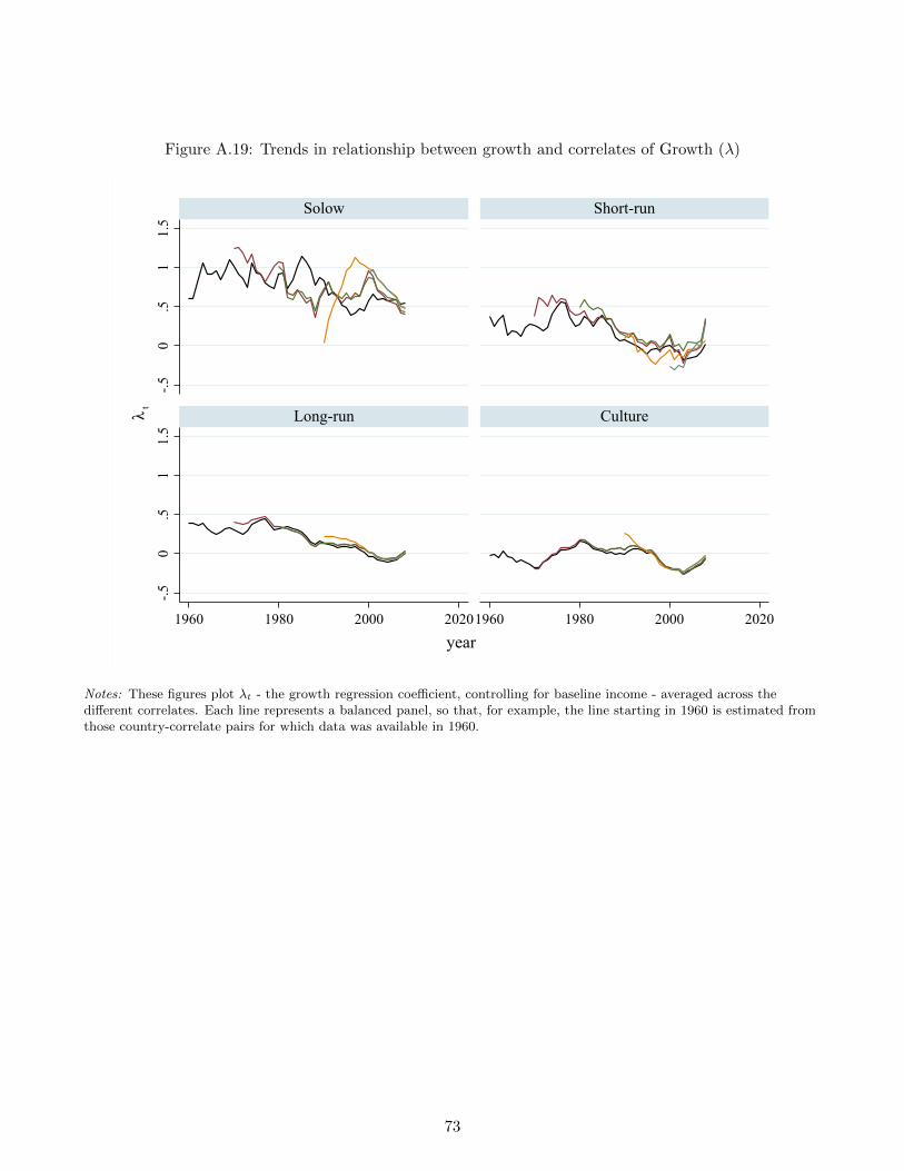
Figure A.19: Trends in relationship between growth and correlates of Growth (λ)-.5
0.5
11.
5-.5
0.5
11.
5
1960 1980 2000 20201960 1980 2000 2020
Solow Short-run
Long-run Cultureλ t
year
Notes: These figures plot λt - the growth regression coefficient, controlling for baseline income - averaged across thedifferent correlates. Each line represents a balanced panel, so that, for example, the line starting in 1960 is estimated fromthose country-correlate pairs for which data was available in 1960.
73
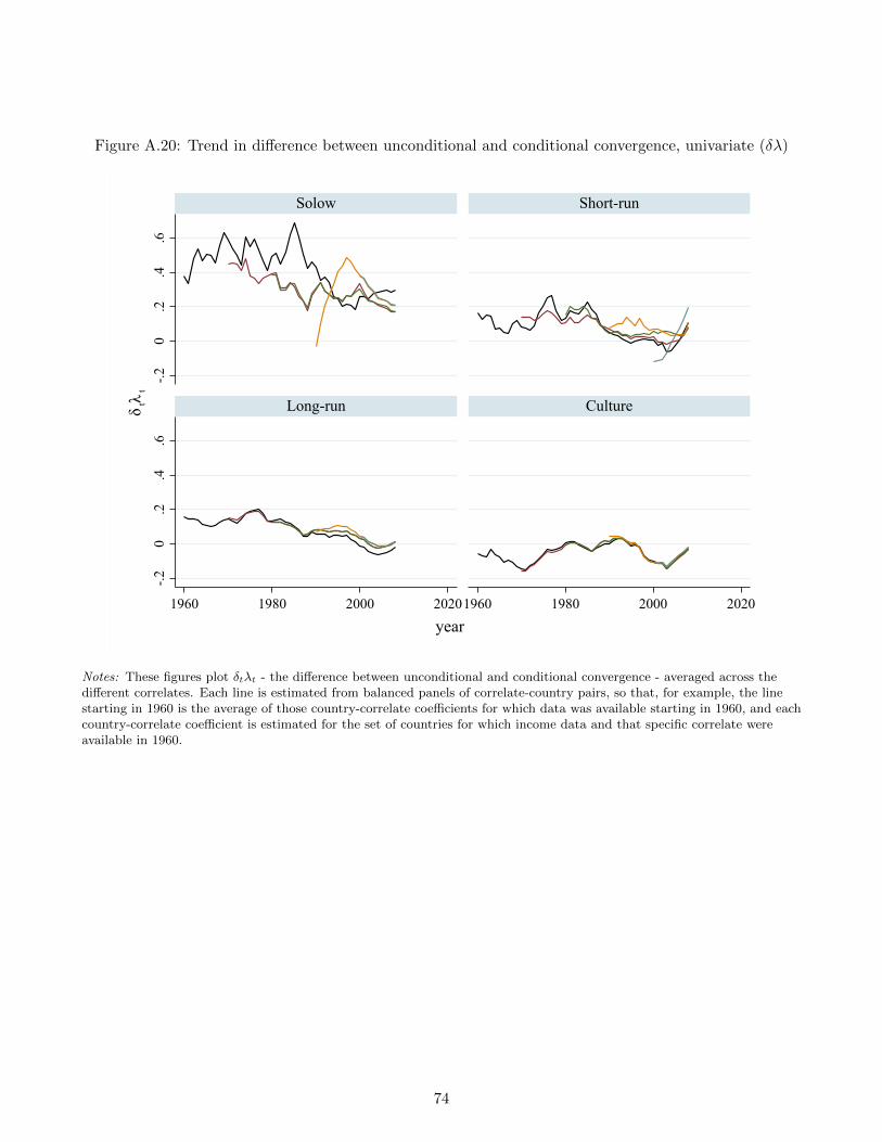
Figure A.20: Trend in difference between unconditional and conditional convergence, univariate (δλ)-.2
0.2
.4.6
-.20
.2.4
.6
1960 1980 2000 20201960 1980 2000 2020
Solow Short-run
Long-run Cultureδ tλ t
year
Notes: These figures plot δtλt - the difference between unconditional and conditional convergence - averaged across thedifferent correlates. Each line is estimated from balanced panels of correlate-country pairs, so that, for example, the linestarting in 1960 is the average of those country-correlate coefficients for which data was available starting in 1960, and eachcountry-correlate coefficient is estimated for the set of countries for which income data and that specific correlate wereavailable in 1960.
74


