
Corpus sta*s*cs: key issues and controversies
Panel Discussion
1

The panellists
• Vaclav Brezina (Lancaster) • Stefan Evert (Erlangen-‐Nürnberg) • Stefan Th. Gries (Santa Barbara) • Andrew Hardie (Lancaster) • Jefrey Lijffijt (Bristol) • Gerold Schneider (Zürich/Konstanz) • Sean Wallis (London) Session chair: MC Paul Rayson (Lancaster)
2

Topics
1. Experimental design: Which factors should we measure?
2. Non-‐randomness, dispersion and the assump*ons of hypothesis tests
3. Teaching and curricula 4. Visualisa*on 5. Which models can we use?
3

1 EXPERIMENTAL DESIGN Sean Wallis, University College London
4

Are we ge_ng sta*s*cs right?
• In a single recent top CL journal volume: – 1 ar*cle employed a method using a per-‐word baseline
• No argument as to why this was op*mal – 1 ar*cle cited a sta*s*cal test without specifying the baseline (expected distribu*on) • Implica*on: constant propor*on of words
– 2 ar*cles quoted naïve frequencies or probabili*es without any inferen*al sta*s*cal evalua*on • Arguably one of these was jus*fied in doing so
5

The centrality of experimental design
• Experimental design is central: – Clarifica*on of testable hypotheses – Abstrac*on / opera*onalisa*on
• Map corpus events to regular dataset • Frequently necessary to reformulate
– The experimental model determines: • instances of phenomena to capture • how to express aspects of phenomena as variables • the appropriate sta*s*cal model
6

The centrality of experimental design
• Experimental design is central: – Clarifica*on of testable hypotheses – Abstrac*on / opera*onalisa*on
• Map corpus events to regular dataset • Frequently necessary to reformulate
– The experimental model determines: • instances of phenomena to capture • how to express aspects of phenomena as variables • the appropriate sta*s*cal model
Annota8on
Abstrac8on
Analysis
Corpus
Text
Dataset
Hypotheses
3A model of Corpus Linguistics (Wallis and Nelson 2001) 7
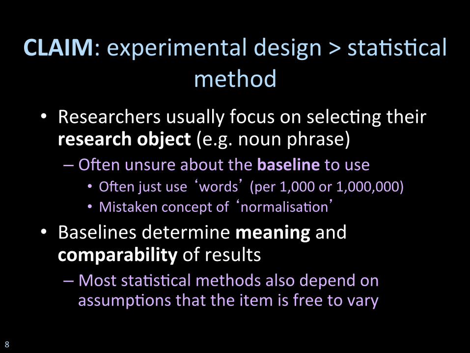
CLAIM: experimental design > sta*s*cal method
• Researchers usually focus on selec*ng their research object (e.g. noun phrase) – Oien unsure about the baseline to use
• Oien just use ‘words’ (per 1,000 or 1,000,000) • Mistaken concept of ‘normalisa*on’
• Baselines determine meaning and comparability of results – Most sta*s*cal methods also depend on assump*ons that the item is free to vary
8

Research ques*ons and baselines • Suppose you are told that – cycling is ge_ng safer
• Do you believe them? – would you start cycling?
• Facts – fatali*es have increased
• What is the most meaningful sta*s*c? – p (accident | popula*on) – p (accident | cyclist) – p (accident | journey) – p (accident | km)
See e.g. hnp://cyclinginfo.co.uk/blog/323/cycling/how-‐dangerous-‐is-‐cycling
9

cyclists
car passengers/drivers
motorcyclists
pedestrians
other vehicles
Research ques*ons and baselines • Suppose you are told that
– cycling is ge_ng safer • Do you believe them?
– would you start cycling? • Facts
– fatali*es increased – are there more
cyclists now? – BUT...
10

cyclists
car passengers/drivers
motorcyclists
pedestrians
Research ques*ons and baselines • Suppose you are told that – cycling is ge_ng safer
• Do you believe them? – would you start cycling?
• Facts – fatali*es increased – there are more cyclists now
– BUT… death rates per km have fallen
11

Baselines alter sta*s*cal models • Logis*c ‘S’ curve assumes freedom to vary – p (X) ∈ [0, 1]
0
1
t
p
12

Baselines alter sta*s*cal models • Logis*c ‘S’ curve assumes freedom to vary
– what happens if that freedom is limited?
– p (X) ∈ [0, ?]
0
1
t
p
opportunity use
13

Baselines alter sta*s*cal models • Logis*c ‘S’ curve assumes freedom to vary
– what happens if that freedom is limited? – or the opportunity to use a construc*on also varies?
– p(X) ∈ [0, ?]
0
1
t
p opportunity
use
14
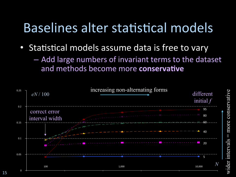
Baselines alter sta*s*cal models • Sta*s*cal models assume data is free to vary
– Add large numbers of invariant terms to the dataset and methods become more conserva8ve
100 1,000 10,000 0
0.05
0.1
0.15
0.2
0.25
5
20 40 60 80 95
eN / 100
N
correct error interval width
different initial f
increasing non-alternating forms
wid
er in
terv
als =
mor
e co
nser
vativ
e
15

Discussion
1. Experimental design: Which factors should we measure?
2. Non-‐randomness, dispersion and the assump*ons of hypothesis tests
3. Teaching and curricula 4. Visualisa*on 5. Which models can we use?
16

2 NON-‐RANDOMNESS Jefrey Lijffijt, University of Bristol
17

The problem
• Sta*s*cal tests/models are always based on assump*ons
• What if the assump*ons are false?
• How would you know?
• What to do?
18

An example problem
• 𝜒2, log-‐likelihood ra*o / G, Fisher Exact test, etc., assume independence of all counts
à Expecta*on of variance over texts (binomial distribu*on)
• Unless samples contain at most one instance, such as extremely short texts (tweets), this expecta*on is always wrong
(Church, COLING 2000, Evert, ZAA 2006, Lijffijt et al., DSH 2014)
19
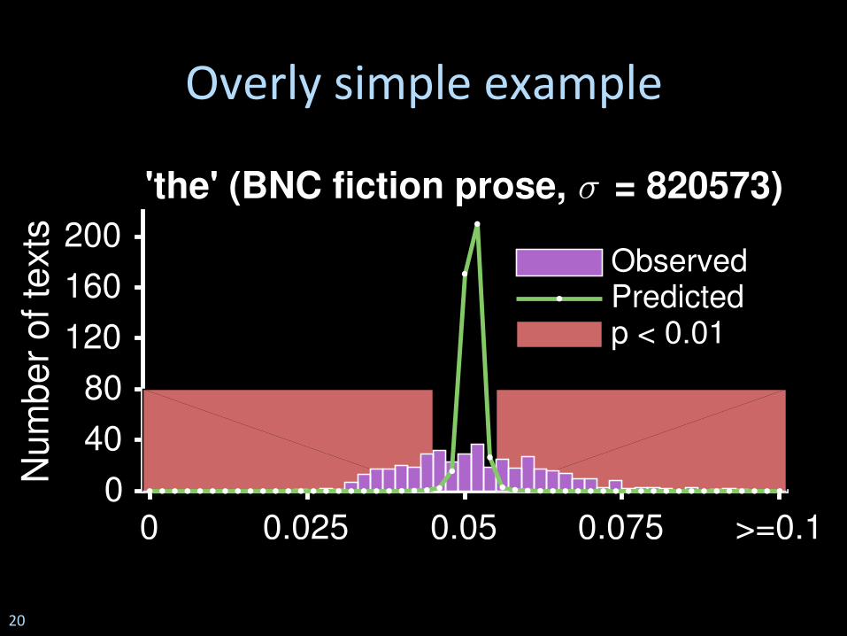
Overly simple example
0 0.025 0.05 0.075 >=0.1
0
40
80
120
160
200
Nu
mb
er
of
texts
'the' (BNC fiction prose, σ = 820573)
Observed
Predicted
0 0.025 0.05 0.075 >=0.10
40
80
120
160
200
Nu
mb
er
of
text
s
'the' (BNC fiction prose, σ = 820573)
ObservedPredictedp < 0.01
20

Sta*s*cs vs. the truth
• ‘Language is never, ever, ever, random’ (Kilgarriff, CLLT 2005)
[These models are very far from the truth à you failed to model the `true’ varia*on]
• Why to model text as random process – Corpus is sample of texts (= true randomness) – Complex structure (= remaining varia*on)
21

Tests and assump*ons
• p = Pr(T ≥ x) – Probability that the test sta*s*c is the same or higher in random data
– This assumes a stochas*c model for the r.v. T
• 𝜒2, log-‐likelihood ra*o / G, Fisher Exact test assume independence of every instance
Y = true Y = false X = true R S X = false T U
22

Why the problem maners
• If the assump*ons are false, p-‐values can be too high or too low, to any degree
• Conjecture: p-‐values derived under invalid assump*ons do not add any value
• The assump*ons underlying a sta*s*cal test have to be correct
23

However
• Some tests require invalid assump*ons –/–> sta*s*cal tes*ng is an ill choice
• Oien, there are alterna*ves 1. Manipulate the representa*on (adjusted counts) 2. Select only appropriate data (use dispersion) 3. Use another test
(t-‐test, anova are almost always fine)
24

The open ques*ons
• Oien, there are alterna*ves 1. Manipulate the representa*on (adjusted counts) 2. Select only appropriate data (use dispersion) 3. Use another test
• What approach to prefer?
• What if it is not clear how to do any of the above?
25

A SECOND OPINION Stefan Evert, Friedrich-‐Alexander-‐Universität Erlangen-‐Nürnberg
26

Three views of corpus studies
• Topic 1: controlled experiment – is there a significant difference btw condi*ons?
• Topic 2: observa*onal study – inference about property of popula*on – problem of non-‐randomness (≠ random text!)
• Topic 5: predic*ve model – which factors affect linguis*c behaviour?
27

Methodological ques*ons
• Do corpus + sta*s*cal analysis accurately reflect the underlying popula*on? – sta*s*cs: yes, if corpus = truly random sample
• What property do we want to measure? – and is it the one we're actually measuring?
☞ popula*on parameter vs. sample sta*s*c
28

Example 1: frequency comparison
• Passive VPs more frequent in BrE than AmE – 13.3% vs. 12.6% ➞ significant? – chi-‐squared: yes!; t-‐test: no!; GLM: yes!!
●
●●
●
●
●
●
●●
●
●
●●
●
●
●
●●
●
●
●
●
●
●
●
●
●
●
●
●
●●●
●
●
●
●
●
●
●
●
●●
●
●
●
●
●
●
●
●
●
●
●●●
●
●
●
●
●
●
●●
●
●
●
●
●
●
●
●
●
●
●
●●
●
●
●
●
●
●
●
●
●●
●
●
●
●
●
●
●
●
●
●
●●
●
●
●
●
●
●
●
●
●
●●●
●
●●
●
●
●
●
●
●
●
●
●●●
●
●
●●
●
●
●
●
●
●
●
●
●
●
●
●
●
●
●
●●
●●
●
●
●
●
●
●●
●
●
●
●
●●
●
●
●
●
●
●
●
●
●
●●
●
●
●
●
●●●
●
●
●
●
●●
●
●
●
●
●
●
●
●●
●
●
●
●
●●
●
●
●
●
●
●
●
●
●
●
●
●
●
●
●
●
●
●
●
●
●
●●
●
●
●
●
●
●
●
●●
●
●●
●●
●●
●
●
●●
●
●
●
●
●
●
●
●●●
●
●
●
●
●
●
●
●
●
●
●
●
●
●
●
●
●
●
●
●
●
●
●
●
●
●●
●
●
●
●●
●
●
●
●
●
●
●
●
●
●
●
●
●
●
●
●
●
●
●●
●
●
●
●
●
●
●
●
●
●
●
●
●
●
●
●
●
●
●
●
●
●
●
●
●
●
●
●
●
●
●
●
●
●
●
●
●
●
●
●
●
●
●
●
●
●
●
●
●
●
●
●
●
●
●
●
●
●
●
●
●
●
●
●
●
●
●
●
●
●
●
●
●●
●
●
●
●
●
●●
●
●
●●
●
●
●
●
●
●
●
●
●●
●●
●
●●
●
●
●
●
●
●
●
●
●
●
●
●●●
●
●●
●●
●
●
●
●●
●
●
●
●
●
●●
●●●●
●●
●●
●●
●
●
●
●
●
●
●●
●
●
●
●
●
●
●
●
●●
●
●
●●
●
●
●
●
●
●
●
●
●
●
●
●
●
●
●
●
●
●
●
●●
●
●
●
●
●
●
●
●
●
●
●
010
2030
4050
6070
Genre variation of passive frequency in Brown/LOB corpus
relat
ive fr
eque
ncy (
%)
pres
s rep
pres
s ed
revie
wsre
ligio
nho
bbies
pop
lore
belle
s let
t
misc
learn
ed
fictio
n
dete
ctive
sci−f
iad
vent
ure
rom
ance
hum
our
●
ukus
29

●
●
●
●
●●
● ●●
●
●●
●●
● ● ● ●● ●
5 10 15 20
01
23
45
geography (N) [clumpiness: 0.6%]
frequency
log 1
0(n d
oc)
● observedbinomial
Example 2: burs*ness
• Content words tend to occur in “bursts”
• P(f = 1) = α(1 – γ) (Katz 1996) P(f = 2) = αγ / (1 – p) P(f = k) = αγ × pk–2 / (1 – p) for k ≥ 3
• Which of α, γ, p is “frequency”? 30

Example 3: dispersion
• Many dispersion measures (e.g. Gries 2008) • Clear: binomial sample = perfect dispersion
31

Example 3: dispersion
• Many dispersion measures (e.g. Gries 2008) • Clear: binomial sample = perfect dispersion
32

Discussion
1. Experimental design: Which factors should we measure?
2. Non-‐randomness, dispersion and the assump*ons of hypothesis tests
3. Teaching and curricula 4. Visualisa*on 5. Which models can we use?
33

3 TEACHING & CURRICULA Vaclav Brezina, Lancaster University
34

Teaching and curricula
View 1: 1. CL is a quan*ta*ve discipline. 2. Efficient quan*fica*on requires
detailed knowledge of sta*s*cs. Hence: CL requires detailed knowledge of sta8s8cs.
35

Teaching and curricula (cont.)
View 2 (loose syllogism): 1. CL combines linguis*cs and
quan*ta*ve (sta*s*cal) methods. 2. Corpus linguists primarily specialise in
understanding linguis*c processes. Hence: It’s good to have an expert sta8s8cian on the team.
36

Example: log likelihood
37

Discussion
1. Experimental design: Which factors should we measure?
2. Non-‐randomness, dispersion and the assump*ons of hypothesis tests
3. Teaching and curricula 4. Visualisa*on 5. Which models can we use?
38

4 VISUALISATION Stefan Th. Gries, University of California, Santa Barbara
39

On why we need to visualize
40

On ink-‐to-‐informa*on ra*o
animate inanimate of 20 40 s 50 15
41

On perspec*ves and uncertainty
42

On granularity
43
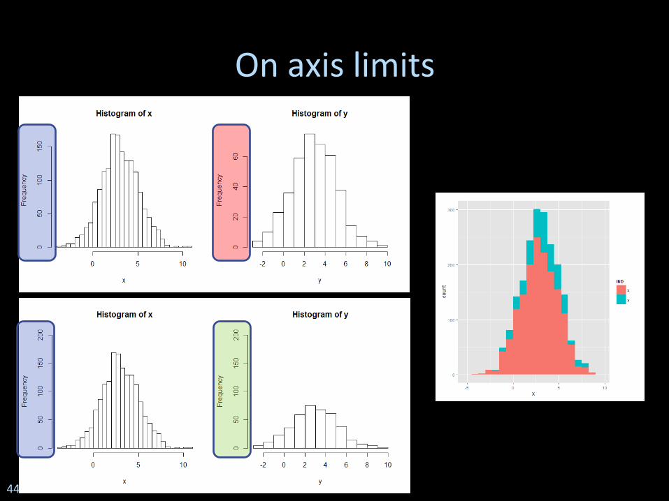
On axis limits
44

On axis limits and on uncertainty
45

On curvature
46

A SECOND OPINION – VISUALISATION AND GOOD SCIENTIFIC PRACTICE
Jefrey Lijffijt, University of Bristol
47
The aim of info-‐vis
1. Enable efficient explora*on of data
2. Discover panerns
• Exploratory data analysis ≠ (just) graphs
• Corpus linguists are great data explorers
48
Inspec*ng raw data
49
[Figure removed in order to respect copyrights]

Querying/playing with data (CQPweb, WordSmith Tools, …)
50

Panern discovery (Sketch Engine)
51

Panern discovery (Phrase Net, GraphColl, …)
52

Finding typical raw data (ProtAnt)
53

Summary
• Graphics can be very helpful
• For big data, graphs are oien necessary
• But, please do not forget to carefully inspect your raw data
54

Discussion
1. Experimental design: Which factors should we measure?
2. Non-‐randomness, dispersion and the assump*ons of hypothesis tests
3. Teaching and curricula 4. Visualisa*on 5. Which models can we use?
55

5 WHICH MODELS? Gerold Schneider, Universität Zürich & Universität Konstanz
56

Which models can we use? Violated assump*on | Improvement • Random distribu*on | Models of choice ó frequency • Independence | Mul*factorial models • Idiosyncra*c Data | Predic*ve models
à Regression à Machine learning
• Characteris*cs of models – Model fit – Evalua*on – Get to know your data!
57

Which models can we use? • Random distribu*on | Models of choice ó frequency
Labov 1969, Church 2000, Evert 2006, Sean Wallis’ Baseline • e.g. passives: per ar*cle | restricted to transi*ve verbs
Per article passive percentages in Brown family 4
filepassORactBrown$p.pass
Density
0.0 0.2 0.4 0.6 0.8 1.0
0.0
0.5
1.0
1.5
2.0
2.5
58

Which models can we use? • Independence / discourse | Mul*factorial models
Gries 2006, Gries 2010, Gries 2015 • e.g. genre (here Brown passives)
●
●
●
●
●
●
●
●
●●●●
●
●
●●
●
●
●●●●
●
●
●●
●●
●●●
A B C D E F G H J K L M N P R
0.0
0.2
0.4
0.6
0.8
Per article passive percentages in Brown family 4 scientific (J)
filepassORactBrown.Jall4$p.pass
Density
0.0 0.2 0.4 0.6 0.8 1.0
0.0
0.5
1.0
1.5
2.0
2.5
59

Which models can we use? • Independence | Mul*factorial models • Genre and subgenre -‐> regression
Per article passive percentages in w2a:1−10(HUM) vs w2a:21−30(NAT)
filepassORactICE.w2a[filepassORactICE.w2a$subgenre == "w2a:1−10", 10]
Den
sity
0.0 0.2 0.4 0.6 0.8 1.0
0.0
0.5
1.0
1.5
2.0
2.5
3.0
filepassORactBrown.J4.subgenreregionperiod= ! aov(p.pass ~ subgenre * region * period, ! data=filepassORactBrown.J4); !summary(filepassORactBrown.J4.subgenreregionperiod) ! Df Sum Sq Mean Sq F value Pr(>F) !subgenre 3 1.7816 0.5939 29.126 7.37e-15 *** !region 1 0.1218 0.1218 5.975 0.0157 * !period 1 0.4852 0.4852 23.795 2.74e-06 *** !subgenre:region 3 0.0876 0.0292 1.433 0.2356 !subgenre:period 3 0.0821 0.0274 1.343 0.2628 !region:period 1 0.0350 0.0350 1.714 0.1924 !subgenre:region:period ! 3 0.0624 0.0208 1.021 0.3853 !Residuals 148 3.0176 0.0204 !
60

Which models can we use? • Predic*ve models: Machine learning
“Depending on defini*onal boundaries, predic*ve modelling is synonymous with, or largely overlapping with, the field of machine learning, as it is more commonly referred to in academic or research and development contexts.” (Wikipedia)
• Regression, naïve Bayes, SVM, … • There is a vast selec*on
of tools out there.
61

Which models can we use? • Predic:ve models
– Data loss and compression / smoothing and generalisa*on – Effect sizes – Generalising power – Permits evalua*on on different / held-‐out dataset
à Evaluate! Get to know your data! – Massive feature set / feature selec*on – Interpretability vs. complexity of algorithm
• Computa*onal linguis*cs tools: – Taggers – Parsers – Machine Transla*on – Distribu*onal Seman*cs – ... – Different methods give complementary views (ML). Triangulate!
62

Which models can we use? • Characteris*cs of models: Feature engineering
e.g. US party speech features from CORPS corpus:
63

Which models can we use? • Characteris*cs of model: Model fit / predic*on accuracy • A bad accuracy can mean:
– You have a bad model. Get more features and seman*c classifica*ons (manual or automated) and take interac*ons into account
– There is no panern here. People have truly free choice, there is no story to be found. Your models aims to fit random distribu*on
– The problem that you are dealing with is really challenging and deserved further, detailed research
– You have some serious outliers in your data • A good accuracy can mean:
– I have a good model which respects all important factors – I have overfined the data – My problem is trivial – The decisions are already taken in my features –> independence?
• Use model fit as parameter, e.g. model fit of my syntac*c parser is higher on corrected learner corpus than on original learner corpus
64

Which models can we use? • Characteris*cs of models: Model fit as parameter: Learner English:
parser scores = model fit is higher on corrected data
65

Which models can we use? – Models! Mul*factorial! Many! ML! – Get to know your data. Evalua*on and
model refinement / feature selec*on / outlier analysis is a cyclical process.
– Corpus as a bicycle of the mind John Sinclair 2014: “I am advoca*ng that we should trust the text. We should be open to what it may tell us … We should search for models that are especially appropriate to the study of text and discourse. The study of language is moving into a new era in which the exploita*on of modern computers will be at the centre of progress” George Box 1987: “all models are wrong, but some are useful”
66

Discussion
1. Experimental design: Which factors should we measure?
2. Non-‐randomness, dispersion and the assump*ons of hypothesis tests
3. Teaching and curricula 4. Visualisa*on 5. Which models can we use?
67

GENERAL DISCUSSION
68

Thank you!
69

Sta*s*cal guidelines from Nature Every ar*cle that contains sta*s*cal tes*ng should state - the name of the sta*s*cal test, - the n value for each sta*s*cal analysis, - the comparisons of interest, - a jus*fica*on for the use of that test (including, for
example, a discussion of the normality of the data when the test is appropriate only for normal data),
- the alpha level for all tests, whether the tests were one-‐tailed or two-‐tailed, and
- the actual P value for each test (not merely "significant" or "P < 0.05"). It should be clear what sta*s*cal test was used to generate every P value. Use of the word "significant" should always be accompanied by a P value;
hnp://www.nature.com/srep/publish/guidelines


