
www.elsevier.com/locate/jpetscieng
Journal of Petroleum Science and Engineering 38 (2003) 37–56
Coupled fluid flow and geomechanical deformation modeling
Susan E. Minkoff a,*, C. Mike Stoneb,1, Steve Bryantc,2,Malgorzata Peszynskac,2, Mary F. Wheelerc,2
aDepartment of Mathematics and Statistics, University of Maryland, Baltimore County, 1000 Hilltop Circle, Baltimore, MD 21250, USAbComputational Solid Mechanics and Structural Dynamics Department 9142, Mail Stop 0847, Sandia National Laboratories,
Albuquerque, NM 87185, USAcCenter for Subsurface Modeling, Texas Institute for Computational and Applied Mathematics (TICAM), The University of Texas at Austin,
Austin, TX 78712, USA
Received 11 April 2002; accepted 3 February 2003
Abstract
Accurate prediction of reservoir production in structurally weak geologic areas requires both mechanical deformation and
fluid flow modeling. Loose staggered-in-time coupling of two independent flow and mechanics simulators captures much of the
complex physics at a substantially reduced cost. Two 3-D finite element simulators—Integrated Parallel Accurate Reservoir
Simulator (IPARS) for flow and JAS3D for mechanics—together model multiphase fluid flow in reservoir rocks undergoing
deformation ranging from linear elasticity to large, nonlinear inelastic compaction. The loose coupling algorithm uses a high-
level driver to call the flow simulator for a set of time steps with fixed reservoir properties. Pore pressures from flow are used as
loads for the geomechanics code in the determination of stresses, strains, and displacements. The mechanics-derived strain is
used to calculate changes to the reservoir parameters (porosity and permeability) for the next set of flow time steps. Mass is
conserved in the coupled code despite dynamically changing reservoir parameters via a modification to the Newton system for
the flow equations, and an approximate rock compressibility becomes a useful preconditioner to help with convergence of the
modified flow equations. Two numerical experiments illustrate the accuracy of the coupled code. The first example is a quarter-
five-spot waterflood undergoing poroelastic deformation, which is validated against a fully coupled simulator. Vertical
displacements at the well locations match to within 10%. Moreover, experimentation shows that 13 mechanics time steps (taken
over the course of 5 years of simulation time) were sufficient to achieve this result (a substantial cost savings over full coupling
in which both the mechanics and flow equations must be solved at each time step). The second numerical example is based on
real data from the Belridge Field in California, which illustrates one of the complex plastic constitutive relationships available in
the coupled code. The results mimic behavior which was observed in the field. The coupled code serves as a prototype for
loosely coupling together any two preexisting simulators modeling diverse physics. This technique produces a coupled code
relatively quickly and inexpensively and has the advantage of accurately modeling complex nonlinear phenomena often
0920-4105/03/$ - see front matter Crown Copyright D 2003 Published by Elsevier Science B.V. All rights reserved.
doi:10.1016/S0920-4105(03)00021-4
* Corresponding author. Tel.: +1-410-455-3029; fax: +1-410-455-1066.
E-mail addresses: [email protected] (S.E. Minkoff), [email protected] (C.M. Stone), [email protected] (S. Bryant),
[email protected] (M. Peszynska), [email protected] (M.F. Wheeler).1 Fax: +1-505-844-9297.2 Fax: +1-512-232-2445.

S.E. Minkoff et al. / Journal of Petroleum Science and Engineering 38 (2003) 37–5638
observed in a real field but difficult to capture with a fully coupled simulator. Further, the code has produced promising results
when used for time-lapse studies of compactible reservoirs.
Crown Copyright D 2003 Published by Elsevier Science B.V. All rights reserved.
Keywords: Coupled processes; Simulation; Mechanics; Flow; Deformation; Petroleum engineering
1. Introduction example, pore pressures might be sent from the flow
To understand the response of reservoirs located in
structurally weak geologic formations, engineers must
use coupled flow simulation and mechanical defor-
mation modeling. While the majority of reservoirs are
located in stable rock formations that do not undergo
deformation, there are many reasons to investigate
coupled flow and geomechanics. Even over-pressur-
ized reservoirs located in stable environments may
undergo ‘‘settling’’ at the start of production. Coupled
flow and mechanics are necessary for predicting well
failures and guiding well placement and production.
Modeling of offshore reservoirs near salt bodies can
also be modeled effectively in this way.
There are three basic algorithms for multiphysics
simulation: full coupling, loose coupling, and one-
way coupling. To define a fully coupled simulator, a
single set of equations (generally a large system of
nonlinear coupled partial differential equations) incor-
porating all of the relevant physics must be derived.
As an example, the traditional porous flow equations
for a rigid matrix would be modified to include terms
for mechanical deformation. Full coupling is often the
preferred method for simulating multiple types of
physics simultaneously since it should theoretically
produce the most realistic results. Unfortunately,
deriving a fully coupled multiphase flow simulator
that models nonlinear, inelastic mechanical deforma-
tion is extremely difficult. Thus with fully coupled
models, one generally simplifies to single-phase flow
and even more commonly, simplifies the mechanics to
linear elasticity (Lewis and Sukirman, 1993a,b; Lewis
and Ghafouri, 1997; Osorio et al., 1999).
At the other end of the spectrum is one-way
coupling in which two essentially separate sets of
equations are solved independently over the same
total time interval. Periodically, output from one
simulator is passed as input to the other; however,
information is passed in only one direction. For
code to load the mechanics calculation of stresses,
strains, and displacements. No information would be
passed back from mechanics to flow, however. In
most practical applications, the two simulators are in
fact run independently. One can often gain valuable
insight into the physical situation from one-way
coupling, and it is clearly preferable (in situations
where mechanics is important) to fluid flow alone. A
very successful one-way coupling experiment was
performed to predict well failures in the Belridge
Field, California. This work included a 200-well fluid
flow simulation intended to help with prediction of
well failure rates in other parts of the field (Fredrich et
al., 1996, 1998).
The present work describes a ‘‘loose coupling’’
algorithm situated somewhere between full and one-
way coupling. In loose coupling, there are two sets of
equations which are solved independently (as in one-
way coupling), but information is passed at desig-
nated time intervals in both directions between the
two simulators (fluid flow and geomechanics). Loose
coupling has the advantage of being relatively simple
to implement (like one-way coupling), but it holds
promise for capturing much more of the complex
nonlinear physics, and thus is closer to a fully
coupled approach. Loose coupling capitalizes on
decades of algorithm and code development in differ-
ent application domains while yielding a coupled
model in much less time than would be required to
create a fully coupled model. Two independently
developed simulators were coupled together: fluid
flow from the University of Texas at Austin (IPARS)
and mechanics from Sandia National Labs (JAS3D).
IPARS can map faults and contains multiple physical
flow models that can run in different parts of the
reservoir domain in a single simulation. JAS3D can
handle large, nonlinear inelastic deformation and
sliding contact surfaces (as well as numerous other
types of mechanics).

S.E. Minkoff et al. / Journal of Petroleum Science and Engineering 38 (2003) 37–56 39
The loose coupling algorithm is similar in spirit to
the methods described in the papers of Fung et al.
(1994), Settari and Mourits (1994), and Settari and
Walters (1999). One of the fundamental questions in
loose coupling is how to best handle large jumps in
flow simulation parameters coming from infrequent
calls to mechanics (relative to the total number of flow/
mechanics time steps used in a fully coupled ap-
proach). Modifications to the flow equations can be
made which allow dynamic changes to flow parame-
ters while still maintaining conservation of mass. The
paper begins with a description of the two simulators
and an explanation of how each simulator was modi-
fied to allow incorporation of parameter updates from
the other simulator. Two numerical experiments illus-
trate the accuracy and efficiency of the loose coupling
scheme. The first experiment is a waterflood validation
of the coupled code against a fully coupled poroelastic
simulator. The loosely coupled simulator is run multi-
ple times using a range of different mechanics time
steps and the results are compared to the fully coupled
simulator output. This experiment demonstrates that
loose coupling can capture much of the physics of full
coupling at considerably less cost. The second numer-
ical example is based on data from the Belridge Field
Fig. 1. Flow chart for loose
in California—a field that underwent considerable
nonrecoverable plastic deformation.
2. Loose coupling vs. other algorithms
The loose coupling algorithm is shown as a flow
chart in Fig. 1. A high-level interface loosely couples
these two simulators by invoking one simulator and
then the other repeatedly over the total simulation time.
The user designates a time step for switching from
flow to mechanics (Dt1, where Dt1 = t1� t0; a typical
value of Dt being anywhere from 1 month to 1 year).
The flow simulator runs for the designated time
interval Dt1 and will most likely break the Dt1 time
interval into multiple time steps. At the end of the time
interval Dt1, the pore pressure is passed to the mechan-
ics code, and the mechanics code then runs the
simulation for that same (prior) Dt1 time interval.
The geomechanics code may take only one time step
for this time interval (or at least different sub-time
steps relative to the flow simulator). The pore pres-
sures used as loads allow the mechanics code to
calculate strains and ultimately updates to porosity
and permeability for the flow simulator’s subsequent
coupling algorithm.
S.E. Minkoff et al. / Journal of Petroleum Science and Engineering 38 (2003) 37–5640
time steps. (For details on the calculation of updated
flow parameters, refer to Sections 4 and 5.) Using the
updated values of flow parameters from mechanics
(time step Dt1), fluid flow is simulated for the next time
interval Dt2 = t2� t1. The two-way staggered-in-time
coupling algorithm proceeds until both simulators
reach the final time tend.
Between the flow and mechanics simulations in
Fig. 1, there is a column devoted to mapping output
and input quantities from one simulator to the other.
This column is necessary because the loose coupling
algorithm does not require the two simulators to use
the same computational grid. In fact, one of the
advantages of loose coupling is that mechanics and
flow need not have identical spatial grids. The flow
domain is typically a subset of the mechanics domain.
The flow simulator should only model the reservoir,
while the mechanics code may need to extend further
in the lateral directions than the reservoir, will surely
need to extend up to the earth’s surface (for over-
burden loading), and may cover an area below the
reservoir as well. Note that fully coupled simulators
typically assume a single computational domain, so
fluid flow is simulated outside of the reservoir (an
unnecessary calculation). The current algorithm does
not even require the two codes to have the same grid
spacing in the parts of the domain where there is
overlap (the reservoir). Physically, there may be a
sound reason why the spatial discretization on the
flow side will differ from that for mechanics (exam-
ples: multiple material layers in the reservoir or a need
for finer resolution to capture complex physics).
Many upscaling and downscaling (or ‘‘averaging’’)
tools are available for mapping quantities from one
grid to another. The loose coupling simulator uses a
software package from Sandia’s engineering suite,
Mapvar (Wellman, 1999). Mapvar provides a few
different methods for accomplishing this mapping,
and the coupled simulator invokes the most robust
method for capturing gradients in the solution: vari-
able values at element centers are scattered to the
nodes via a linear constrained least squares fitting
procedure. For a small sample of the upscaling liter-
ature, refer to Arbogast et al. (1998b), Hou and Wu
(1997), E (1992), Durlofsky (1991), Durlofsky et al.
(1994, 1996), Christie (1996), Christie et al. (1995),
King et al. (1993, 1995), and Espedal and Saevareid
(1994).
3. Description of simulators
3.1. Reservoir simulator
The fluid flow simulator, Integrated Parallel Accu-
rate Reservoir Simulator (IPARS) (Wang et al., 1997;
Parashar et al., 1997; Wheeler et al., 1999), devel-
oped at the University of Texas, is a three-dimen-
sional general subsurface simulator that can be run
serially or in parallel using MPI. It currently includes
multiple physical models: single phase, two-phase
oil–water and air–water, and a reactive transport,
compositional model as well as the black oil model
described below. IPARS contains several numerical
discretizations of these physical models including
mixed finite elements and discontinuous Galerkin
finite elements for two-phase flow. The mixed finite
element method gives a stencil equivalent to cell-
centered finite differences if lowest order Raviart–
Thomas spaces are used for approximation and the
computational domain is rectangular (Russell and
Wheeler, 1983; Arbogast et al., 1996, 1997). The
scheme allows for discontinuity and for degeneracy
of fluid–rock properties, and it has optimal conver-
gence properties (Arbogast et al. 1996, 1997, 1998a).
Additionally, different time discretizations have been
implemented in IPARS including implicit, semi-
implicit, and sequential.
The IPARS simulator was chosen for this work
because of its unusual capabilities which are well
suited to coupled flow and mechanics. One such
feature allows the user to break the physical domain
into subdomains corresponding to geologic blocks
and then to apply different gridding or even different
physical or numerical flow models to each block. As
an example, certain production scenarios might best
be understood via flow simulation which uses a
compositional model. However, a black oil model
might suffice for the parts of the reservoir domain far
from the production wells. A version of domain
decomposition mortar space-based methodology,
originally formulated for single-phase flow (Arbogast
et al., 1996; Yotov, 1998), was developed to ensure
convergence across interfaces between these different
subdomain blocks and models (Peszynska et al.,
1999, 2002; Wheeler et al., 2000; Lu et al., 2001).
IPARS’ unique capacity to follow geologic structure
(especially faults) via blocking makes it a good

S.E. Minkoff et al. / Journal of Petroleum Science and Engineering 38 (2003) 37–56 41
choice for a sophisticated flow and mechanics simu-
lator.
Although the IPARS framework makes it relatively
easy to port code changes between different flow
models, in this work the black oil model is used
exclusively. Black oil is the simplest model which
includes all three fluid phases (oil, gas, and water)
needed for seismic time-lapse studies (Minkoff et al.,
1999). In this black oil model, the reservoir is
assumed to be isothermal, the permeability tensor is
diagonal, and the viscosity of each phase is constant.
No chemical reactions, precipitation, or adsorption are
present, and the formation is slightly compressible.
The external boundary conditions are no-flow Neu-
mann conditions. Numerically, the black oil model
code is fully implicit, 3-D, and uses an expanded
mixed finite element method to maintain local con-
servation of mass (Lu, 2000; Lu et al., 2001).
3.1.1. Black oil formulation
Assume that two or three phases and three compo-
nents are present. The uppercase subscripts W, O, and
G are used for the fluid components: water, heavy
hydrocarbon or oil, and light hydrocarbon or gas,
respectively. Lowercase subscripts w, o, and g are
used for the fluid phases: aqueous, oleic, and gaseous
phase, respectively. The model is partially miscible. In
particular, the water component exists only in the
water phase and it is the only component in that
phase. The gas phase contains only the gas component
and may be absent if the pressure is high enough, and
the oil phase may contain both the oil and gas
components. The oil component is the residual liquid
at atmospheric pressure after differential vaporization,
while the gas component is the remaining fluid
(Peaceman, 1977; Lake, 1989).
Given that NI is the stock tank volume of compo-
nent I (I=O,G,W) per unit pore volume, / is porosity,
Ro is the stock tank volume of gas dissolved in a stock
tank volume of oil, and qI is the total stock tank rate of
injection of component I, the mass balance equations
are
B
Btð/NGÞ ¼ �r � ðUg þ RoUoÞ þ qG
B
Btð/NI Þ ¼ �r � Ui þ qI I ¼ oil; water ð1Þ
Darcy’s Law gives the mass velocity U of phase i
(here i= oil, gas, or water):
Ui ¼ � Kkri
Bili
� ðrPi � qigrDÞ ð2Þ
Here, K is the absolute permeability tensor, and kriis the relative permeability of phase i. Bi is the
formation volume factor for phase i. Pi is pressure,
li is viscosity, and qi is density. Gravity has magni-
tude g, and D is depth. Finally, the saturations must
satisfy the constraint:
Sg þ So þ Sw ¼ 1
and capillary pressures are defined by
PcowðSwÞ ¼ Po � Pw
PcgoðSgÞ ¼ Pg � Po
The gas component is soluble in the oil phase. The
maximum concentration of gas that can be dissolved in
the oil phase at a given pressure is given by Rs. The
subscript s stands for ‘‘saturated’’ conditions, and Rs is
an increasing function of pressure. If the amount of gas
contained in some element of volume is less than this
maximum (Ro <Rs), then all the gas dissolves into the
oil phase, so that Sg = 0. If the amount of gas in the
element exceeds this maximum, then Ro =Rs, and a free
gas phase exists, so that Sg>0. Reducing the pressure of
a volume of gas-saturated oil causes gas to come out of
solution and form a free gas phase. Thus two-phase and
three-phase conditions may prevail simultaneously in
different regions of the same reservoir.
The state equations complete the formulation.
Denote the stock tank density of component I by qIS.
Then, the water density is given by qw = qWS/Bw and
the density of the gas phase (if it exists) is given by
qg = qGS/Bg. Both the equations Sw = BwNW and
Sw = 1� So� Sg define the water phase saturation.
The oil phase density and saturation are related by
So =BoNO and qo=(qOS +RoqGS)/Bo. Finally, gas satu-
ration in three-phase conditions is Sg =Bg(NG�RsNO).
3.2. Geomechanical deformation modeling
The geomechanics code from Sandia National
Laboratories, JAS3D, is a three-dimensional, quasi-

S.E. Minkoff et al. / Journal of Petroleum Science and Engineering 38 (2003) 37–5642
static finite element code. Like IPARS for fluid flow,
JAS3D is a mechanical deformation code with sev-
eral unique capabilities. Specifically, JAS3D can
accurately model large deformations, sliding contact
surfaces, and both elastic and inelastic material
responses from a wide array of constitutive models
(Arguello et al., 1998). The advanced finite element
technology which is used in JAS3D is based on
iterative quasistatic solvers which allow problems
with large numbers of unknowns to be efficiently
solved.
3.2.1. Traditional vs. explicit finite element approach
Consider the following field equation governing
the deformation of a body occupying a volume, V,
Brij=Bxj þ qf i ¼ 0 on V : ð3Þ
Eq. (3) is the quasi-static equation of motion,
where rij is the Cauchy stress tensor, xj is the position
vector, q is the mass per unit volume, and fi is aspecific body force vector. The solution to Eq. (3)is sought subject to the kinematic and tractionboundary conditions
hiðx; tÞ ¼ Hiðx; tÞ on VU ð4Þ
rijnj ¼ siðx; tÞ on VT ð5Þ
where VU represents the portion of the boundaryon which kinematic quantities are specified (i.e.,displacements, hi), nj is a unit normal vector, andVT represents the portion of the boundary onwhich tractions are specified. The boundary of thebody is given by the union of VU and VT.
For the displacement-based finite element method,
the equations described in the foregoing paragraph
can be discretized and rewritten in one of two ways:
XN
Zve
BsdV
( )¼ fFg ð6Þ
and
½KðhÞ�fhg ¼ fFg; ð7Þ
where the term on the left-hand side of Eqs. (6) and
(7) is the internal force vector, and {F} is the external
force vector. In Eq. (6), B is the strain-displacement
transformation matrix, N is the number of elements in
the finite element method (FEM) discretization, s is
an ordered vector of stress components in each
element at a Gauss point, and ve is the volume of
each element. In Eq. (7), [K(h)] represents the global
stiffness matrix and {h} represents the global vector
of unknown nodal displacements. Both Eqs. (6) and
(7) are included to highlight the difference in
approach between the traditional FEM approach and
the local-iterative approach used in this work.
The traditional FEM approach involves the direct
solution of Eq. (7). Namely, an element stiffness and
external force vector are formed for each element in
the overall structure. The contributions from each of
these element stiffness matrices and force vectors are
then assembled into a global stiffness matrix and force
vector describing the overall system. For the inelastic
and/or geometrically nonlinear case (the stiffness
matrix varies with the unknowns), the load is typically
applied incrementally. The resulting nonlinear equa-
tions are then solved at each load increment with some
variant of the Newton–Raphson method. The direct
factorization of this sparse global stiffness matrix can
result in (1) extremely large storage requirements and
(2) a very large number of arithmetic operations,
especially for three-dimensional problems. Commer-
cially available software is generally limited and will
typically only handle models on the order of tens of
thousands of elements in size. When attempting to
solve large problems of interest to the oil and gas
industry, models on the order of hundreds of thou-
sands to millions of elements may be needed. For
problems of this size, the traditional direct solution
approach becomes prohibitive due to memory and
computational time requirements.
The iterative technology that is used in JAS3D
never requires the formation of a global stiffness
matrix. Instead, the divergence of the stress is found
at the element level. Contributions to each node in the
overall structure are summed (i.e., the vector described
by the left side of Eq. (6)). A residual force vector
made from the internal minus the external forces,
fRg ¼XN
Zve
BsdV
( )� fFg; ð8Þ
is computed, and the solution procedure is then one of
reducing the residual to zero using an iterative techni-

S.E. Minkoff et al. / Journal of Petroleum Science and Engineering 38 (2003) 37–56 43
que. Because the quantities being manipulated are
vectors, there is no need to store or factor a global
stiffness matrix. Consequently, the storage require-
ments are small when compared to the traditional
FEM approach. Two iterative techniques are currently
used in JAS3D—a preconditioned conjugate gradient
technique (Biffle, 1993) and an adaptive dynamic
relaxation technique (Stone, 1997). These two iterative
techniques are both able to handle the nonlinearities
associated with inelastic material response and sliding
contact surfaces. Comparing performance of a com-
mercially available FEM program against JAS3D on
an inelastic problem with 250,000 elements, the tradi-
tional FEM code took 30 times more CPU time than
was required to solve the same problem using JAS3D.
4. Modifications to fluid flow
Traditional flow simulators initialize porosity and
permeability at the start of the computation and then
these quantities remain fixed throughout the simula-
tion. For coupled flow and mechanics, these quantities
must be updated each time the code completes a
JAS3D step.
4.1. Porosity updates
In traditional flow simulators, small changes to
reservoir rock properties (porosity /) are accounted
for by the following linear expression:
/ ¼ /*ð1þ crðP � P*ÞÞ ð9Þ
where /* is the initial porosity at initial pressure P*,
and rock compressibility cr is a constant (typically on
the order of 10� 7–10� 10 Pa� 1). The code uses water
pressure, Pw, in place of pore pressure since water is
the phase wetting the rock and thus a reasonable
choice. A saturation-weighted average of the three
fluid phase pressures also could be used. In reality,
conventional black oil simulators assume that the
reservoir geology (porosity and permeability) is
changing very little (if at all) during flow simulation.
In the coupled simulations, Eq. (9) is not used to
determine porosity (although it is used for precondi-
tioning the solver, as described below). Porosity
values at the beginning of each set of simulation time
steps are input to the flow simulator from the mechan-
ics portion of the code, as depicted in Fig. 1.
The nonlinear system resulting from the finite
element discretization of Eqs. (1) and (2) is solved
via Newton’s method. Writing this system in matrix
form gives Jx =�R, with J the Jacobian matrix of
partial derivatives with respect to the primary varia-
bles x=[Pw,NO,NG], and R the residual. The solution
vector x actually contains incremental changes in the
primary variables.
Recalling a representative equation from the mass
balance system for component a, the residual is
Ra ¼ /ðNnþ1a � Nn
a Þ þ dtðr � Unþ1a � qnþ1
a Þ ð10Þ
with the backward Euler method used for the time
discretization. For coupled geomechanics and reser-
voir simulation, porosity updates at time step n + 1 are
introduced through the residual modification
Ra ¼ ð/NaÞnþ1 � ð/NaÞn þ dtðr � Unþ1a � qnþ1
a Þ:ð11Þ
In other words, the porosity values at time step
n+ 1 are provided by the mechanics code and directly
incorporated into the Newton system to be solved. In
the above formulation, mass is conserved, and the
Newton update accounts for a decrease in pore space
(for example) by increasing the well rates and pres-
sures at the next time step.
4.2. Permeability updates
Dynamic updates of absolute permeability during
flow simulation impact large portions of the code. The
grid block transmissibilities in the discretized equa-
tions and parts of the well model must be continu-
ously updated.
Rewriting Eq. (11) slightly, the water phase equa-
tion becomes:
ð/NWÞnþ1 � ð/NWÞn
Dtnþ1þr � Unþ1
w ¼ qnþ1w ð12Þ
The oil and gas phase equations are similar. In the
equation above, Dt n + 1 = t n + 1� t n. The correspond-
S.E. Minkoff et al. / Journal of Petroleum Science and Engineering 38 (2003) 37–5644
ing nonlinear residual equation used in Newton’s
method is
RKw;ijk ¼ Vijkfð/NWÞKijk � ð/NWÞnijk þ Dtnþ1
� ½r � Uw � qw�Kijkg: ð13Þ
The subscript ijk refers to the grid cell indexed by i
in the x direction, j in the y direction, and k in the z
direction. The superscript K refers to the Kth approx-
imation to the superscripted quantity at time level
n + 1. The volume of grid cell ijk is denoted Vijk.
From Darcy’s Law (Eq. (2)), the component mass
velocities in the residual equation above are discre-
tized using cell-centered differencing in space,
Dtnþ1Vijkðj � UwÞKijk ¼ �kKw;iþ1=2; jk
hPKw;iþ1; jk � PK
w;ijk
� qKw;iþ1=2; jkgðDiþ1; jk � DijkÞ
iþ kKw;i�1=2; jk
hPKw;ijk � PK
w;i�1;jk
� qKw;i�1=2; jkgðDijk � Di�1; jkÞ
iþ similar terms for the y and
z directions:
If Kxx, Kyy, and Kzz are harmonically averaged
values of the absolute permeability tensor between
adjacent grid cells, and Dxi, Dyj, and Dzk are the edge
lengths of a rectangular grid cell ijk, then the trans-
missibility constants that appear in the upstream-
weighted mobility computation for k are:
kKw;iþ1=2; jk ¼ Dtnþ12DyjDzkDxi
Kxx;ijkþ Dxiþ1
Kxx;iþ1; jk
� ��1
� krw
Bwlw
� �K
sjk
where s = i if Pw,ijkK zPw,i + 1, jk
K , and s = i+ 1 if Pw,ijkK <
Pw,i + 1, jkK . Upstream weighting is used similarly in the
y and z directions.
The values of transmissibility are generally as-
sumed fixed in uncoupled flow simulators. Here, they
must be updated after each mechanics step to account
for the permeability changes induced by strain. In the
coupled code, permeability also must change dynam-
ically in the well model. IPARS currently allows for
two types of wells: bottom-hole pressure specified and
rate specified (Peaceman, 1983; Lu, 2000). The volu-
metric rate of flow of fluid phase i (i=w,o,g) from the
well bore to a grid cell can be expressed as
Qi ¼GLKkri
li
ðPwb � PiÞ ð14Þ
where Pwb is the well-bore pressure (hydrostatic
pressure), Pi is the pressure of phase i in the grid cell,
K is the absolute permeability of the grid cell, L is the
length of the open well bore penetrating the grid cell,
and G is a dimensionless geometric factor related to
the well-bore radius and given by the Peaceman
(1983) correction.
5. Modifications to mechanics
5.1. Porosity updates
The mechanics code is capable of calculating
pointwise changes in pore volume in the reservoir,
coming (for example) from field production, pressure
decrease, and then compaction. To calculate these
field property changes in the coupled code, the
reservoir simulator sends the pore pressure field to
the geomechanics part of the code where it is used in
the calculation of total stress:
rTij ¼ rij þ pdij:
Here p is the pore fluid pressure, dij is the Kro-
necker delta function, and rij is the ‘‘effective’’ stresswhich is used in the constitutive model. The total
stress is used in the determination of the equilibrium
state for the reservoir subject to the overburden loads,
kinematic boundary conditions, and changing pore
pressure field. On output, the geomechanics code
provides an updated porosity, /, at the current time
step via the following expression:
/ ¼ 1� ð1� /0Þeev
where /0 is the initial porosity, and ev is the total
volume strain (the sum of the elastic and inelastic
components of strain). JAS3D uses a description for
the motion of the continuum that is valid for the large
deformation response of the reservoir rock.

S.E. Minkoff et al. / Journal of Petroleum Science and Engineering 38 (2003) 37–56 45
5.2. Permeability updates
Using available permeability-differential stress
data for several different rock types, a correlation
can be established between permeability and total
volume strain. The volume strain captures the pre-
failure permeability decline as well as the large post-
failure permeability reduction. After experimenting
with several different functional forms relating per-
meability to volume strain, an exponential model that
gave the best data fit was chosen:
K ¼ AeBev :
Here A and B are material constants and ev is again
the total volume strain. Because additional experimen-
tal data to define an anisotropic permeability tensor is
not available, the change in the permeability expres-
sion is assumed to be isotropic. Given the requisite
measured data, however, any other functional form for
permeability could be substituted into the code.
6. Convergence issues—a Newton’s method
preconditioner for the coupled code
Although loose coupling enables modeling of
realistic physics much more cheaply than full cou-
pling (fewer mechanics time steps must be taken), this
time savings is not for free. When the reservoir
parameters change dynamically with time, the flow
equations become more difficult to solve. After each
JAS3D step, IPARS receives new values of perme-
ability and porosity which are used for the next set of
flow time steps. If mechanical deformation is linear
elastic and the rock compressibility relationship relat-
ing porosity to pressure described by Eq. (9) holds,
then the flow solver will have little difficulty search-
ing for the next solution to the Newton system. By
differentiating Eq. (9) with respect to pressure,
changes in pore volume are estimated. This expres-
sion guides the flow solver towards a solution for the
next time step. In the coupled code, mechanical
deformation is not restricted to be linear elastic.
JAS3D has a range of over 50 constitutive relation-
ships for modeling deformation (Appendix A). This
flexibility in material modeling, however, requires
IPARS to grapple with incorporating a set of numbers
(representing updated reservoir parameters) without
any information about the way in which the flow
problem has changed. This lack of information can
cause the IPARS solver to have difficulty converging.
To improve the convergence of the flow solver in the
coupled code, the rock compressibility expression is
reintroduced solely for the purpose of preconditioning
the flow equations in IPARS. In other words, the user
provides an approximate value for compressibility
which is used to determine the derivative of Eq. (9)
with respect to pressure. This derivative is used in
forming the Jacobian for the Newton system. The
actual values of reservoir porosity used in the flow
equations still come entirely from the JAS3D compu-
tations, however. This strategy greatly improves
IPARS’ chances of converging after JAS3D time steps
in which the reservoir properties change substantially
with time.
7. Numerical examples
7.1. Validation experiment
The first numerical example in this paper is a
validation experiment in which output from IPARS/
JAS3D is compared to the solution from a fully
coupled ARCO simulator, ACRES (Dean et al.,
2003). ACRES uses finite differences to discretize
the multiphase flow problem and finite elements for
the mechanics calculation (displacements). The
poroelastic equations are formulated in terms of total
stresses, bulk strains, and fluid pressures. The non-
linear flow equations and linear poroelastic equations
are fully coupled and solved iteratively using a New-
ton–Raphson technique. The Newton–Raphson me-
thod linearizes the equations which are then passed to
a linear solver. The resulting matrix system is solved
for block pressures, well pressures, and displace-
ments.
The validation experiment is based on a waterflood
with the domain containing one production well and
one injection well—each of which is located in an
opposite corner of the grid (a ‘‘quarter-five-spot
pattern’’). The waterflood simulation covers 25 years
with a specified water injection rate of 79.5 m3/day
and production rate for liquids of 119 m3/day. The
production well is also assigned a limit of 3.45 MPa

S.E. Minkoff et al. / Journal of Petroleum Science and Engineering 38 (2003) 37–5646
(below which the bottom-hole pressure cannot fall).
The average reservoir pressure will decline during
simulation (producing compaction in the field) as the
production rate is greater than the injection rate.
In this example, mechanical deformation is
restricted to be elastic with reservoir compressibility
of 1.1603� 10� 8 Pa� 1. (The pore compressibility is
about the same magnitude as the total fluid compres-
sibility in this case.) Poisson’s ratio is set at 0.3, and
Biot’s constants a and M� 1 have values of 1 and 0,
respectively. The reservoir’s top surface is at a depth
of 1414 m, and the computational domain extends
402 m in the x direction, 402 m in the y direction,
and 61 m in z (depth). The domain is discretized into
20� 20� 10 cells. Boundary conditions for the
external grid edges are no-flow and zero displace-
ment. The initial porosity is set at 30% throughout
the reservoir. The horizontal permeability varies from
5 to 100 md in depth. Initial fluid saturations for the
reservoir are 20% water and 80% oil, with no free
gas. The average reservoir pressure is 21.03 MPa
initially with bubble point pressure for the fluid set at
20.79 MPa.
Fig. 2. Contour plot of gas saturation (dimensionless) from IPARS/JAS3D a
Experiment 1). The front corner of the domain contains the production
simulation, the reservoir contains no free gas. Production causes a drop i
ACRES uses an incomplete LU preconditioner
(Strang, 1986) with generalized conjugate residual
iteration to solve the linear equations for pressure
and a direct solver for displacements. ACRES time
steps varied from 0.01 to 5 days. IPARS linearizes the
coupled set of flow equations via Newton’s method
and then solves the resulting linear system using a
GMRES solver (Axelsson, 1994) with multi-level
preconditioner (Edwards, 1998). The GMRES solver
had a tolerance of 1�10� 4, the Newton solver a
tolerance of 1�10� 6. Time steps in IPARS ranged in
duration from 1 to 10 days.
As expected, the reservoir pressure drops through-
out the field because the rate of production exceeds
that of injection. The rate of decrease is not uniform,
however. A gradient is produced between the two
wells. The greatest pressure decrease (and hence
porosity decrease and displacements) occurs at the
production well, and the least change occurs at the
injection well. In this experiment, permeability is held
fixed at the initial values throughout the simulation in
order to facilitate comparison to ACRES. Fig. 2 shows
gas saturation contours from the IPARS/JAS3D simu-
t the end of the 25-year waterflood validation simulation (Numerical
well. The back corner contains the injection well. At the start of
n pressure and the formation of gas in the reservoir.

S.E. Minkoff et al. / Journal of Petroleum Science and Engineering 38 (2003) 37–56 47
lation at 25 years. Initially there is no gas in the field,
but as the pore pressure drops below the bubble point
pressure during production, gas comes out of solution
changing the problem from two- to three-phase flow.
At the end of the simulation, the field contains 27% gas
near the production well. In a similar fashion, oil
pressure contours depicted in Fig. 3 show an overall
pressure drop in the field (from initial pressures of
20.68 MPa) with the largest decrease at the production
well (where the final pressures are around 4.69 MPa).
At the injection well the final pressures are about twice
this value 8.96 MPa. Finally, Fig. 4 shows the change
in porosity at 25 years. The initial reservoir porosity
was homogeneous at 30%. The final porosities show a
decrease of almost 13% over the initial simulation
porosities (giving values near the production well of
less than 26%).
In order to test the sensitivity of the results to the
frequency of mechanics steps, a suite of six IPARS/
JAS3D simulations was run. The first two experi-
ments took 15- and 30-day mechanics time steps,
respectively. As the output was essentially identical
between these two simulations, additional runs were
performed with 90-day, 1-year, 2-year, and 5-year
mechanics time steps. The ‘‘critical time step’’ for
Fig. 3. Contour plot of oil pressure (MPa) from IPARS/JAS3D at the end o
of the domain contains the production well. The back corner contains the in
of simulation.
mechanics for this experiment seems to be 2 years. In
other words, the simulations with mechanics time
steps ranging from 15 days all the way up to 2 years
produced the same IPARS/JAS3D displacement his-
tories at the wells. When the mechanics time steps
were lengthened to 5 years, however, a noticeable
change appeared in the loosely coupled solution.
Fig. 5 compares vertical displacement at the two
well locations (producer and injector) for ACRES vs.
IPARS/JAS3D. The three black curves correspond to
vertical displacement histories at the production well.
The three red curves correspond to vertical displace-
ments at the injection well. The dashed red and black
curves are the ACRES displacements. The solid red
and black curves are the IPARS/JAS3D simulation
results for five of the six simulations (JAS3D time
steps of 15 days, 30 days, 90 days, 1 year, and 2 years).
Finally, the red and black dashed curves with super-
imposed geometric shapes correspond to the vertical
displacement histories resulting from the IPARS/
JAS3D simulation with 5-year JAS3D time steps.
The dashed (ACRES) and solid (IPARS/JAS3D) lines
are qualitatively similar with a quantitative discrep-
ancy of approximately 10% which is most likely due to
remaining differences in the ACRES and IPARS flow
f the 25-year validation simulation (Experiment 1). The front corner
jection well. The average reservoir pressure is 21.03 MPa at the start

Fig. 4. Contour plot of porosity (dimensionless) from IPARS/JAS3D at the end of the 25-year validation simulation (Experiment 1). The front
corner of the domain contains the production well. The back corner contains the injection well. Porosity is uniform at 30% throughout the
reservoir at the start of simulation.
S.E. Minkoff et al. / Journal of Petroleum Science and Engineering 38 (2003) 37–5648
solutions. This figure shows that for this 25-year
simulation, no difference exists between taking 13
mechanics time steps and taking 600 (every 2 years
or every 15 days). This example illustrates the benefits
of loose coupling. The simulation captures the funda-
mental physics at a tiny fraction of the cost of running
a fully coupled simulation. When the mechanics time
steps are lengthened to every 5 years, however, the
loosely coupled simulation results diverge substan-
tially from the fully coupled result. At 10 years (the
second mechanics time step), IPARS/JAS3D is able to
recover back to the smaller IPARS/JAS3D time step
solution (and hence to the fully coupled ACRES
solution). More complicated models for mechanics
(plastic) might not be so easy to match with such long
mechanics time steps in the loosely coupled model and
would require further investigation.
7.2. Single layer Belridge experiment
The second example is based on data from the
Belridge Field west of Bakersfield, CA. The field was
estimated to have more than 500 Mm3 of original oil-
in-place. The field contains two reservoirs: a smaller
reservoir located in the shallow Tulare sand, and a
slightly deeper reservoir located in diatomite and
extending nearly 305 m in depth. Despite the fact that
this large diatomite reservoir was discovered in the
early 1900s, by the mid-1990s, most of the production
was still focused on the Tulare reservoir (Fredrich et
al., 1996). The diatomite has unusual geologic proper-
ties which make production difficult. This reservoir
has very high porosities ranging from 45% to 70%,
but very low permeability (f 0.1 md). In the mid-
1970s, hydraulic fracturing allowed production in this
field for the first time. With increased production
came substantial subsidence, however (up to 6 m at
the earth’s surface in places), and hence well failures
which by the mid-1990s amounted to a well failure
rate of 2–5% annually (Fredrich et al., 1996).
Although the reservoir contains multiple sedimen-
tary layers, for simplicity, the synthetic experiment
models only one of these layers. This layer (J) is the
weakest of the diatomite layers, with an elastic mod-
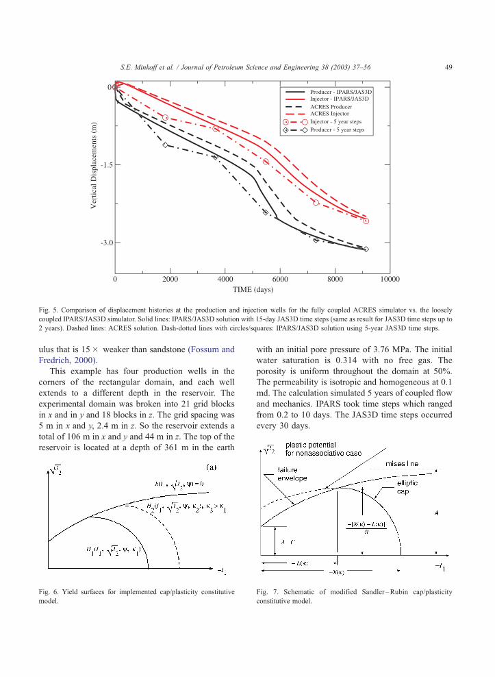
Fig. 5. Comparison of displacement histories at the production and injection wells for the fully coupled ACRES simulator vs. the loosely
coupled IPARS/JAS3D simulator. Solid lines: IPARS/JAS3D solution with 15-day JAS3D time steps (same as result for JAS3D time steps up to
2 years). Dashed lines: ACRES solution. Dash-dotted lines with circles/squares: IPARS/JAS3D solution using 5-year JAS3D time steps.
S.E. Minkoff et al. / Journal of Petroleum Science and Engineering 38 (2003) 37–56 49
ulus that is 15� weaker than sandstone (Fossum and
Fredrich, 2000).
This example has four production wells in the
corners of the rectangular domain, and each well
extends to a different depth in the reservoir. The
experimental domain was broken into 21 grid blocks
in x and in y and 18 blocks in z. The grid spacing was
5 m in x and y, 2.4 m in z. So the reservoir extends a
total of 106 m in x and y and 44 m in z. The top of the
reservoir is located at a depth of 361 m in the earth
Fig. 6. Yield surfaces for implemented cap/plasticity constitutive
model.
with an initial pore pressure of 3.76 MPa. The initial
water saturation is 0.314 with no free gas. The
porosity is uniform throughout the domain at 50%.
The permeability is isotropic and homogeneous at 0.1
md. The calculation simulated 5 years of coupled flow
and mechanics. IPARS took time steps which ranged
from 0.2 to 10 days. The JAS3D time steps occurred
every 30 days.
Fig. 7. Schematic of modified Sandler –Rubin cap/plasticity
constitutive model.
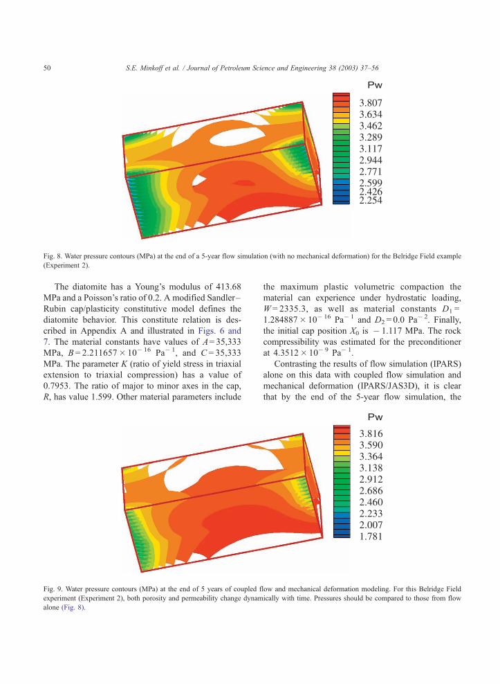
Fig. 8. Water pressure contours (MPa) at the end of a 5-year flow simulation (with no mechanical deformation) for the Belridge Field example
(Experiment 2).
S.E. Minkoff et al. / Journal of Petroleum Science and Engineering 38 (2003) 37–5650
The diatomite has a Young’s modulus of 413.68
MPa and a Poisson’s ratio of 0.2. A modified Sandler–
Rubin cap/plasticity constitutive model defines the
diatomite behavior. This constitute relation is des-
cribed in Appendix A and illustrated in Figs. 6 and
7. The material constants have values of A= 35,333
MPa, B = 2.211657� 10� 16 Pa� 1, and C = 35,333
MPa. The parameter K (ratio of yield stress in triaxial
extension to triaxial compression) has a value of
0.7953. The ratio of major to minor axes in the cap,
R, has value 1.599. Other material parameters include
Fig. 9. Water pressure contours (MPa) at the end of 5 years of coupled f
experiment (Experiment 2), both porosity and permeability change dynam
alone (Fig. 8).
the maximum plastic volumetric compaction the
material can experience under hydrostatic loading,
W = 2335.3, as well as material constants D1 =
1.284887� 10� 16 Pa� 1 and D2 = 0.0 Pa� 2. Finally,
the initial cap position X0 is � 1.117 MPa. The rock
compressibility was estimated for the preconditioner
at 4.3512� 10� 9 Pa� 1.
Contrasting the results of flow simulation (IPARS)
alone on this data with coupled flow simulation and
mechanical deformation (IPARS/JAS3D), it is clear
that by the end of the 5-year flow simulation, the
low and mechanical deformation modeling. For this Belridge Field
ically with time. Pressures should be compared to those from flow

Fig. 10. Equivalent total strain (dimensionless) at the end of the 5-year coupled flow and mechanics simulation of the synthetic Belridge Field
data.
S.E. Minkoff et al. / Journal of Petroleum Science and Engineering 38 (2003) 37–56 51
pressures have decreased by 40% from their initial
values. At the end of the coupled flow and mechanics
simulation, the pressures had decreased by 50%. A
maximum difference in pressure between the two
Fig. 11. Vonmises stress (Pa) at the end of the 5-year coupled flow a
simulations occurs at the production wells (about
0.45 MPa). Refer to Fig. 8 for the pressures from flow
alone and Fig. 9 for the water pressures from coupled
flow and mechanics.
nd mechanics simulation of the synthetic Belridge Field data.

Fig. 12. Displacement (m) at the end of the 5-year coupled flow and mechanics simulation of the synthetic Belridge Field data.
S.E. Minkoff et al. / Journal of Petroleum Science and Engineering 38 (2003) 37–5652
Fig. 10 shows equivalent total strain contours at the
end of the coupled flow and deformation run. Total
strain at the end of the run is 3%. Fig. 11 shows Von
Mises stress for the coupled simulation, and one can
see the 3-D variations in stress at the wells which is
due to different well schedules and different well
completion depths. At the end of 5 years of coupled
simulation, a maximum subsidence of 0.15 m has
Fig. 13. Permeability (md) at the end of the 5-year coupled flow and me
simulation, the permeabilities were 0.1 md uniformly throughout the rese
occurred at the wells (Fig. 12). During coupled
simulation, porosity decreases by 2%, but the perme-
abilities show the biggest change, decreasing from 0.1
to 0.001 md at the wells. Fig. 13 shows the final
permeability at the end of the coupled run.
Feedback occurs when the reservoir parameters
change dynamically during flow. Changes in porosity
and permeability coming from the mechanics code
chanics simulation of synthetic Belridge Field data. At the start of
rvoir.
S.E. Minkoff et al. / Journal of Petroleum Science and Engineering 38 (2003) 37–56 53
impact pressures coming out of flow simulator, which
in turn impact future parameter changes produced by
mechanics. Such nonlinear phenomena are difficult to
predict and are often not evident in uncoupled (or
simple coupled) models.
8. Conclusions
Defining a fully coupled model for complex multi-
phase flow and large nonlinear inelastic mechanical
deformation is costly and time-consuming. An alter-
native is to loosely couple two preexisting flow and
mechanics simulators. Staggered-in-time coupling and
two-way passage of information allow accurate mod-
eling of a range of reservoir conditions. The staggered-
in-time loose coupling scheme alternates between flow
and mechanics. The mechanics simulator produces
updated reservoir parameters which are used by the
flow simulator in the next set of time steps. This
technique has the advantage that the simulation
domains for flow and mechanics can be substantially
different (even within the reservoir). There is no need to
simulate flow in the non-reservoir rocks as often must
be done in full coupling.
The primary bottleneck to this technique is that
only relatively small jumps in porosity can be handled
due to the large volume of fluids which must move to
the wells to conserve mass when compaction occurs
in the field. An approximate rock compressibility
(used only as a Newton’s method preconditioner)
helps guide the flow solver toward a solution when
both porosity and permeability change substantially
with time.
A poroelastic waterflood experiment provides a
validation of the loose coupling scheme against a
fully coupled simulator from ARCO (ACRES). Good
agreement was achieved between ACRES and IPARS/
JAS3D at the wells. In fact, a time-step study revealed
little difference in the coupled solution when the
JAS3D mechanics time steps ranged from 15 days
to 2 years. It is considerably cheaper to do a mechan-
ics simulation once every 2 years than every time a
flow step is taken (as in full coupling). An adaptive
time-stepping strategy for measuring the degree of
nonlinearity in the problem and hence optimizing the
mechanics time step will maximize the cost-saving
benefits of loose coupling.
Nomenclature
Bi formation volume factor for fluid phase i
cr rock compressibility
D depth
fi body force vector
g gravitational acceleration constant
kri relative permeability of phase i
K absolute permeability
Ni stock tank volume of component i
Pi phase pressure
qi injection rate for phase i
Ro stock tank volume of gas dissolved in oil
Rso solution gas ratio
Si phase saturation
Ui fluid phase velocity
xj geomechanics position vector
dij Kronecker delta function
Dt time step
Dx spatial step in x direction
Dy step in y direction
Dz step in z direction
ev total volume strain
hi displacement
k mobility
li viscosity
q density
qis stock tank density of component i
rij Cauchy stress tensor
/ porosity
XU portion of mechanics boundary with kine-
matic constraints
XT portion of mechanics boundary with tractions
Acknowledgements
The authors thank Rick Dean from UT Austin for
his invaluable help with the ACRES validation
experiment. Joe Eaton enriched the project with his
knowledge and enthusiasm. The authors gratefully
acknowledge support for this work from the U.S.
Department of Energy’s Natural Gas and Oil Technol-
ogy Partnership Program (NGOTP). Oil industry
partners for this project include BP, ChevronTexaco,
ExxonMobil, Halliburton, and Schlumberger. The
second author is employed at Sandia National Labo-
ratories. Sandia is a multiprogram laboratory operated
by Sandia Corporation, a Lockheed Martin Company,
S.E. Minkoff et al. / Journal of Petroleum Science and Engineering 38 (2003) 37–5654
for the United States Department of Energy under
contract DE-AC04-94AL85000.
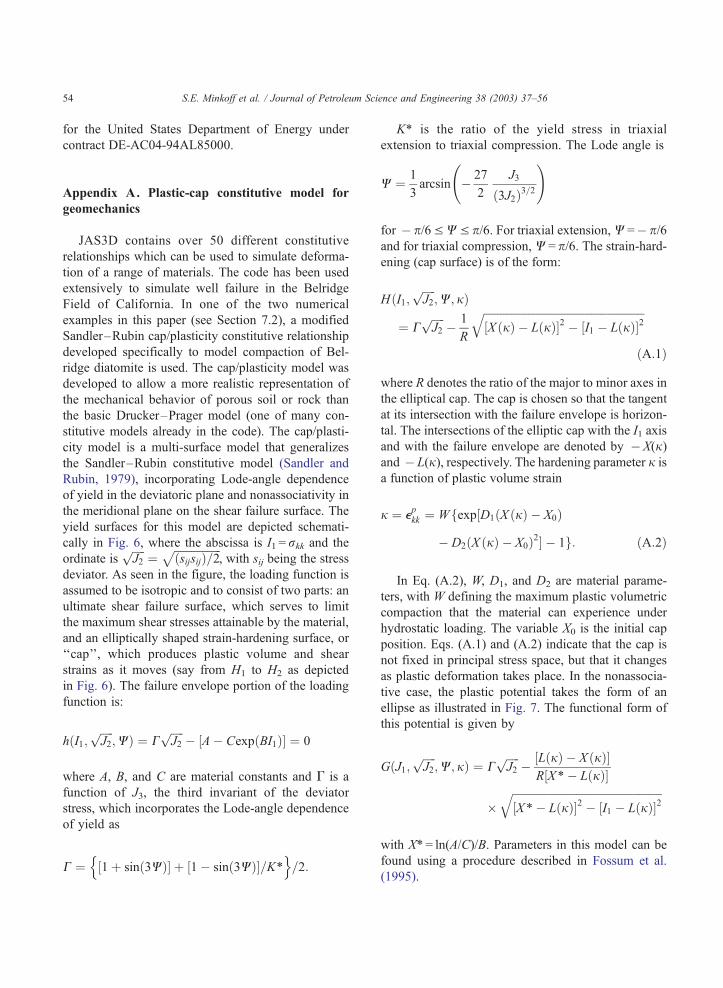
Appendix A. Plastic-cap constitutive model for
geomechanics
JAS3D contains over 50 different constitutive
relationships which can be used to simulate deforma-
tion of a range of materials. The code has been used
extensively to simulate well failure in the Belridge
Field of California. In one of the two numerical
examples in this paper (see Section 7.2), a modified
Sandler–Rubin cap/plasticity constitutive relationship
developed specifically to model compaction of Bel-
ridge diatomite is used. The cap/plasticity model was
developed to allow a more realistic representation of
the mechanical behavior of porous soil or rock than
the basic Drucker–Prager model (one of many con-
stitutive models already in the code). The cap/plasti-
city model is a multi-surface model that generalizes
the Sandler–Rubin constitutive model (Sandler and
Rubin, 1979), incorporating Lode-angle dependence
of yield in the deviatoric plane and nonassociativity in
the meridional plane on the shear failure surface. The
yield surfaces for this model are depicted schemati-
cally in Fig. 6, where the abscissa is I1 = rkk and the
ordinate isffiffiffiffiffiJ2
p¼
ffiffiffiffiffiffiffiffiffiffiffiffiffiffiffiffiffiðsijsijÞ=2
p, with sij being the stress
deviator. As seen in the figure, the loading function is
assumed to be isotropic and to consist of two parts: an
ultimate shear failure surface, which serves to limit
the maximum shear stresses attainable by the material,
and an elliptically shaped strain-hardening surface, or
‘‘cap’’, which produces plastic volume and shear
strains as it moves (say from H1 to H2 as depicted
in Fig. 6). The failure envelope portion of the loading
function is:
hðI1;ffiffiffiffiffiJ2
p;WÞ ¼ C
ffiffiffiffiffiJ2
p� ½A� CexpðBI1Þ� ¼ 0
where A, B, and C are material constants and G is a
function of J3, the third invariant of the deviator
stress, which incorporates the Lode-angle dependence
of yield as
C ¼n½1þ sinð3WÞ� þ ½1� sinð3WÞ�=K*
o=2:
K* is the ratio of the yield stress in triaxial
extension to triaxial compression. The Lode angle is
W ¼ 1
3arcsin � 27
2
J3
ð3J2Þ3=2
!
for � p/6VWV p/6. For triaxial extension, W =� p/6and for triaxial compression, W = p/6. The strain-hard-ening (cap surface) is of the form:
HðI1;ffiffiffiffiffiJ2
p;W; jÞ
¼ CffiffiffiffiffiJ2
p� 1
R
ffiffiffiffiffiffiffiffiffiffiffiffiffiffiffiffiffiffiffiffiffiffiffiffiffiffiffiffiffiffiffiffiffiffiffiffiffiffiffiffiffiffiffiffiffiffiffiffiffiffiffiffiffiffiffiffiffiffi½X ðjÞ � LðjÞ�2 � ½I1 � LðjÞ�2
qðA:1Þ
where R denotes the ratio of the major to minor axes in
the elliptical cap. The cap is chosen so that the tangent
at its intersection with the failure envelope is horizon-
tal. The intersections of the elliptic cap with the I1 axis
and with the failure envelope are denoted by �X(j)and � L(j), respectively. The hardening parameter j is
a function of plastic volume strain
j ¼ epkk ¼ Wfexp½D1ðX ðjÞ � X0Þ
� D2ðX ðjÞ � X0Þ2� � 1g: ðA:2Þ
In Eq. (A.2), W, D1, and D2 are material parame-
ters, with W defining the maximum plastic volumetric
compaction that the material can experience under
hydrostatic loading. The variable X0 is the initial cap
position. Eqs. (A.1) and (A.2) indicate that the cap is
not fixed in principal stress space, but that it changes
as plastic deformation takes place. In the nonassocia-
tive case, the plastic potential takes the form of an
ellipse as illustrated in Fig. 7. The functional form of
this potential is given by
GðJ1;ffiffiffiffiffiJ2
p;W; jÞ ¼ C
ffiffiffiffiffiJ2
p� ½LðjÞ � X ðjÞ�
R½X*� LðjÞ�
�ffiffiffiffiffiffiffiffiffiffiffiffiffiffiffiffiffiffiffiffiffiffiffiffiffiffiffiffiffiffiffiffiffiffiffiffiffiffiffiffiffiffiffiffiffiffiffiffiffiffiffiffiffiffi½X*� LðjÞ�2 � ½I1 � LðjÞ�2
q
with X* = ln(A/C)/B. Parameters in this model can be
found using a procedure described in Fossum et al.
(1995).

S.E. Minkoff et al. / Journal of Petroleum Science and Engineering 38 (2003) 37–56 55
References
Arbogast, T., Wheeler, M., Yotov, I., 1996. Logically rectangular
mixed methods for flow in heterogeneous domains. In: Aldama,
A., et al. (Eds.), Computational Methods in Water Resources XI.
Comp. Mech. Publ., Southampton, UK, pp. 621–628.
Arbogast, T., Wheeler, M., Yotov, I., 1997. Mixed finite elements
for elliptic problems with tensor coefficients as cell-centered
finite differences. SIAM J. Numer. Anal. 34 (2), 828–852.
Arbogast, T., Dawson, C., Keenan, P., Wheeler, M., Yotov, I.,
1998a. Enhanced cell-centered finite differences for elliptic
equations on general geometry. SIAM J. Sci. Comp. 19 (2),
404–425.
Arbogast, T., Minkoff, S., Keenan, P., 1998b. An operator-based
approach to upscaling the pressure equation. In: Burganos, V.,
Karatzas, G., Payatakes, A., Brebbia, C., Gray, W., Pinder, G.
(Eds.), Computational Methods in Water Resources XII. Compu-
tationalMechanics Publication, Southampton, UK, pp. 405–412.
Arguello, J., Stone, C., Fossum, A., 1998. Progress on the develop-
ment of a three-dimensional capability for simulating large-scale
complex geologic processes. Proceedings of the 3rd North
American Rock Mechanics Symposium. ISRM, Rotterdam.
No. USA-327-3.
Axelsson, O., 1994. Iterative Solution Methods. Cambridge Univ.
Press, New York.
Biffle, J., 1993. JAC3D—a three-dimensional finite element com-
puter program for the nonlinear quasistatic response of solids with
the conjugate gradient method. Technical Report, SAND87-
1305, Sandia National Labs, Albuquerque, NM.
Christie, M., 1996. Upscaling for reservoir simulation. J. Pet. Tech-
nol. 48, 1004–1010.
Christie, M.A., Mansfield, M., King, P.R., Barker, J.W., Culver-
well, I.D., 1995. A renormalisation-based upscaling technique
for WAG floods in heterogeneous reservoirs. Proceedings of
the 13th Reservoir Simulation Symposium. SPE 29127,
pp. 353–361. San Antonio, TX.
Dean, R., Gai, X., Stone, C., Minkoff, S., 2003. A comparison of
techniques for coupling porous flow and geomechanics. Pro-
ceedings of the 17th Reservoir Simulation Symposium. SPE
79709. Houston, TX.
Durlofsky, L., 1991. Numerical calculation of equivalent grid block
permeability tensors for heterogeneous porous media. Water
Resour. Res. 27, 699–708.
Durlofsky, L.J., Jones, R.C., Milliken, W.J., 1994. A new method
for the scale up of displacement processes in heterogeneous
reservoirs. Proceedings of the 4th European Conference on the
Mathematics of Oil Recovery. Roros, Norway.
Durlofsky, L.J., Behrens, R.A., Jones, R.C., Bernath, A., 1996.
Scale up of heterogeneous three dimensional reservoir descrip-
tions. SPE J. 1, 313–326.
E, W., 1992. Homogenization of scalar conservation laws with
oscillatory forcing terms. SIAM J. Appl. Math. 52, 959–972.
Edwards, H.C., 1998. A parallel multilevel-preconditioned GMRES
solver for multiphase flow models in the Implicit Parallel Ac-
curate Reservoir Simulator. Texas Institute for Computational
and Applied Math Report. University of Texas, Austin, TX.
Espedal, M.S., Saevareid, O., 1994. Upscaling of permeability
based on wavelet representation. Proceedings of the 4th Euro-
pean Conference on the Mathematics of Oil Recovery. Roros,
Norway.
Fossum, A., Fredrich, J., 2000. Constitutive models for the Etch-
egoin Sands, Belridge Diatomite, and overburden formations
at the Lost Hills Oil Field, California. Technical Report,
SAND2000-0827, Sandia National Labs, Albuquerque, NM.
Fossum, A., Senseny, P., Pfeifle, T., Mellegard, K., 1995. Exper-
imental determination of probability distributions for parameters
of a salem limestone cap plasticity model. Mech. Mater. 21,
119–137.
Fredrich, J., Arguello, J., Thorne, B., Wawersik, W., Deitrick, G.,
de Rouffignac, E., Myer, L., Bruno, M., 1996. Three-dimen-
sional geomechanical simulation of reservoir compaction and
implications for well failures in the Belridge Diatomite. Pro-
ceedings of the SPE Annual Technical Conference and Exhibi-
tion, No. 36698. SPE, Richardson, TX, pp. 195–210.
Fredrich, J., Deitrick, G., Arguello, J., de Rouffignac, E., 1998.
Reservoir compaction, surface subsidence, and casing damage:
a geomechanics approach to mitigation and reservoir manage-
ment. Proceeding of SPE/ISRM EUROCK 1998, No. 47284.
SPE and ISRM.
Fung, L.-K., Buchanan, L., Wan, R.G., 1994. Coupled geome-
chanical – thermal simulation for deforming heavy-oil reser-
voirs. J. Can. Pet. Technol. 33 (4), 22–28.
Hou, T.Y., Wu, X.H., 1997. A multiscale finite element method
for elliptic problems in composite materials and porous media.
J. Comput. Phys. 134, 169–189.
King, P.R., Muggeridge, A.H., Price, W.G., 1993. Renormalization
calculations of immiscible flow. Transp. Porous Media 12,
237–260.
King, M.J., King, P.R., McGill, C.A., Williams, J.K., 1995. Effec-
tive properties for flow calculations. Transp. Porous Media 20,
169–196.
Lake, L.W., 1989. Enhanced Oil Recovery. Prentice-Hall, Engle-
wood Cliffs, NJ.
Lewis, R., Ghafouri, H., 1997. A novel finite element double po-
rosity model for multiphase flow through deformable fractured
porous media. Int. J. Numer. Anal. Methods Geomech. 21,
789–816.
Lewis, R., Sukirman, Y., 1993a. Finite element modelling for sim-
ulating the surface subsidence above a compacting hydrocarbon
reservoir. Int. J. Numer. Anal. Methods Geomech. 18, 619–639.
Lewis, R., Sukirman, Y., 1993b. Finite element modelling of three-
phase flow in deforming saturated oil reservoirs. Int. J. Numer.
Anal. Methods Geomech. 17, 577–598.
Lu, Q., 2000. A parallel multi-block/multi-physics approach for
multi-phase flow in porous media. PhD thesis, University of
Texas at Austin, Austin, TX.
Lu, Q., Peszynska, M., Wheeler, M.F., 2001. A parallel multi-block
black-oil model in multi-model implementation. Proceedings of
the 16th Reservoir Simulation Symposium, No. 66359. SPE,
Richardson, TX.
Minkoff, S., Stone, C., Arguello, J., Bryant, S., Eaton, J., Peszynska,
M., Wheeler, M., 1999. Coupled geomechanics and flow simu-
lation for time-lapse seismic modeling. Proceedings of the 69th
Annual International Meeting. SEG, Tulsa, OK, pp. 1667–1670.

S.E. Minkoff et al. / Journal of Petroleum Science and Engineering 38 (2003) 37–5656
Osorio, J., Chen, H., Teufel, L., 1999. Numerical simulation of the
impact of flow-induced geomechanical response on the produc-
tivity of stress-sensitive reservoirs. Proceedings of the 15th Res-
ervoir Simulation Symposium, No. 51929. SPE, Richardson,
TX, pp. 373–387.
Parashar, M., Pope, G., Wang, K., Wang, P., Wheeler, J., 1997. A
new generation EOS compositional reservoir simulator: Part II.
Framework and multiprocessing. Proceedings of the 14th Reser-
voir Simulation Symposium, No. 37977. SPE, Richardson, TX.
Peaceman, D., 1977. Fundamentals of Numerical Reservoir Simu-
lation. Elsevier, New York.
Peaceman, D., 1983. Interpretation of well-block pressure in numer-
ical reservoir simulation with non-square grid blocks and aniso-
tropic permeability. SPE J. 23 (3), 531–543.
Peszynska, M., Lu, Q., Wheeler, M.F., 1999. Coupling different
numerical algorithms for two phase fluid flow. In: Whiteman,
J.R. (Ed.), Proceedings of Mathematics of Finite Elements and
Applications. Brunel University, Uxbridge, UK, pp. 205–214.
Peszynska, M., Wheeler, M., Yotov, I., 2002. Mortar upscaling
for multiphase flow in porous media. Comput. Geosci. 6 (1),
73–100.
Russell, T., Wheeler, M., 1983. Finite element and finite difference
methods for continuous flows in porous media. In: Ewing, R.E.
(Ed.), The Mathematics of Reservoir Simulation. SIAM, Phila-
delphia, pp. 35–106.
Sandler, I., Rubin, D., 1979. An algorithm and a modular routine
for the cap model. Int. J. Numer. Anal. Methods Geomech. 3,
173–186.
Settari, A., Mourits, F., 1994. Coupling of geomechanics and res-
ervoir simulation models. In: Siriwardane, Zaman (Eds.), Com-
puter Methods and Advances in Geomechanics. Balkema,
Rotterdam, pp. 2151–2158.
Settari, A., Walters, D., 1999. Advances in coupled geomechanical
and reservoir modeling with applications to reservoir compac-
tion. Proceedings of the 15th Reservoir Simulation Symposium,
No. 51927. SPE, Richardson, TX, pp. 345–357.
Stone, C., 1997. SANTOS—a two-dimensional finite element pro-
gram for the quasistatic, large deformation, inelastic response of
solids. Technical Report, SAND90-0543, Sandia National Labs,
Albuquerque, NM.
Strang, G., 1986. Introduction to Applied Mathematics. Wellesley-
Cambridge Press, Wellesley, MA.
Wang, P., Yotov, I., Wheeler, M., Arbogast, T., Dawson, C., Parashar,
M., Sepehrnoori, K., 1997. A new generation EOS compositional
reservoir simulator: Part I. Formulation and discretization.
Proceedings of the 14th Reservoir Simulation Symposium,
No. 37979. SPE, Richardson, TX.
Wellman, G.W., 1999. MAPVAR—a computer program to transfer
solution data between finite element meshes. Technical Report,
SAND99-0466, Sandia National Labs, Albuquerque, NM.
Wheeler, M., Arbogast, T., Bryant, S., Eaton, J., Lu, Q., Peszynska,
M., Yotov, I., 1999. A parallel multiblock/multidomain ap-
proach for reservoir simulation. Proceedings of the 15th Reser-
voir Simulation Symposium, No. 51884. SPE, Richardson, TX,
pp. 51–61.
Wheeler, M., Wheeler, J., Peszynska, M., 2000. A distributed com-
puting portal for coupling multi-physics and multiple domains
in porous media. In: Bentley, L., Sykes, J., Brebbia, C., Gray,
W., Pinder, G. (Eds.), Computational Methods in Water Resour-
ces. A.A. Balkema, Southampton, UK, pp. 167–174.
Yotov, I., 1998. Mortar mixed finite element methods on irregular
multiblock domains. In: Wang, J., et al. (Eds.), Iterative Meth-
ods in Scientific Computation, vol. 4. IMACS, Amsterdam, pp.
239–244.


