Coupling of Electromagnetic Fields to Circuits in a Cavity
D.R. Wilton, D.R. Jackson, C. Lertsirimit
University of Houston
Houston, TX 77204-4005
N.J. Champagne
Lawrence Livermore National Laboratory
Livermore, CA 94550
This research supported by the U.S. Department of Defense
under MURI grant F49620-01-1-0436.

As Part of Our MURI Effort, We Are to Develop Capabilities for Modeling
Complex EMC/EMI Problems
slotPCB
cavity
Airborne Transmitter
Ground-based orship-board Transmitter
PEDSLightning
External Threats
Internal Threats
(Picture from NASA-Langley)

As a First Step, We Want to Determine EIGER’s Suitability for Code Validation and for Performing
General-Purpose EMC/EMI Calculations
• EIGER is a general-purpose EM frequency domain modeling code being jointly developed by
• U. Houston/NASA
• Navy (SPAWAR)
• Lawrence Livermore National Laboratory
• Sandia National Laboratories
• Can EIGER be used to obtain quick results and handle difficult-to-formulate EMC/EMI calculations?
• Can EIGER be used to validate new codes, and to efficiently obtain desired model parameters?
• Can it be used as a breadboard for developing more specialized codes?
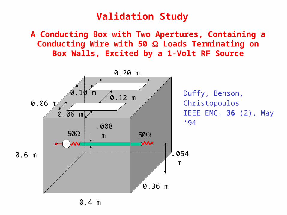
A Conducting Box with Two Apertures, Containing a Conducting Wire with 50 Loads Terminating on Box Walls,
Excited by a 1-Volt RF Source
+ -
0.4 m
0.6 m
0.36 m
.054m
.008m
0.06 m
0.12 m0.06 m
0.10 m
0.20 m
5050
Duffy, Benson, Christopoulos IEEE EMC, 36 (2), May ‘94
Validation Study
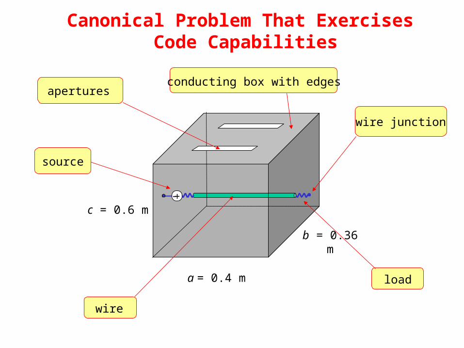
Canonical Problem That Exercises Code Capabilities
+ -
a = 0.4 m
c = 0.6 m
b = 0.36 m
wire junction
apertures
source
wire
load
conducting box with edges
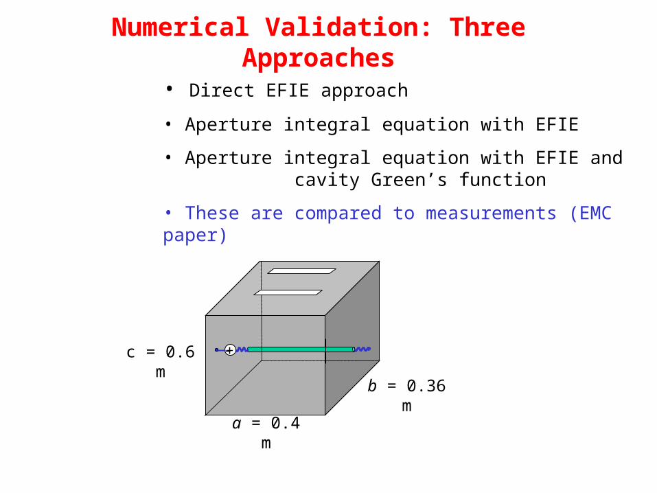
Numerical Validation: Three Approaches
• Direct EFIE approach
• Aperture integral equation with EFIE
• Aperture integral equation with EFIE and cavity Green’s function
• These are compared to measurements (EMC paper)
+ -
a = 0.4 m
c = 0.6 m
b = 0.36 m

Approach #1: Direct EFIE
The system is treated as one conducting object (with source, loads, and junctions)
+-
Js (total current)
I
ˆ , I 0sn E J
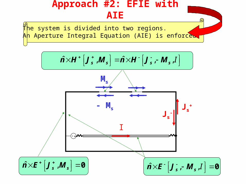
Approach #2: EFIE with AIE
The system is divided into two regions. An Aperture Integral Equation (AIE) is enforced.
+-
Js+
I
ˆ , 0+ +s sn E J M
Ms
- Ms
Js-
ˆ , , I 0- -s sn E J M
ˆ ˆ, , , I + + - -
s s s sn H J M n H J M

Approach #3: EFIE with AIE and Cavity Green’s Function
An AIE is used as in approach 2. A cavity Green’s function is used to calculate the interior fields.
+-
I
- Ms
unit cell
cavity(TOP VIEW)
a
c
a
b
2a
2b
The cavity Green’s function is synthesized by using a sum of four periodic layered-media Green’s functions.Ewald acceleration is used for each one.
ˆ , I 0-sn E M

Results
• Determine normalized output current at opposite end of line excited by a 1 V source
• Compare to measurement (Duffy et al., IEEE Trans. EMC, May 1994, pp. 144 -146)
+ -
0.4 m
0.6 m
0.36 m
.054 m
0.008 m
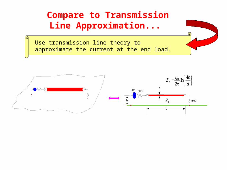
Compare to Transmission Line Approximation...
Use transmission line theory to approximate the current at the end load.
h
d
÷øö
çèæ
d
hZ
4ln
20
0 ph
0Z
1V 50
50
L
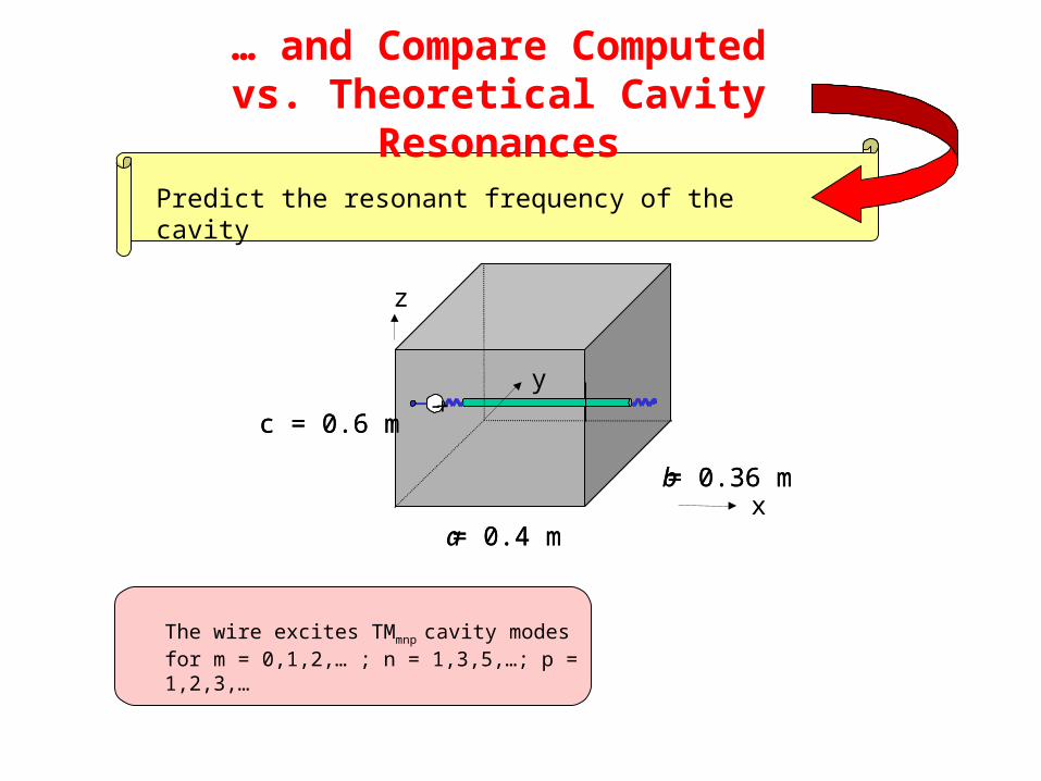
Predict the resonant frequency of the cavity
… and Compare Computed vs. Theoretical Cavity Resonances
The wire excites TMmnp cavity modesfor m = 0,1,2,… ; n = 1,3,5,…; p = 1,2,3,…
+-
a = 0.4 m
c = 0.6 m
b = 0.36 m
+-+-
a = 0.4 m
c = 0.6 m
b = 0.36 mx
y
z
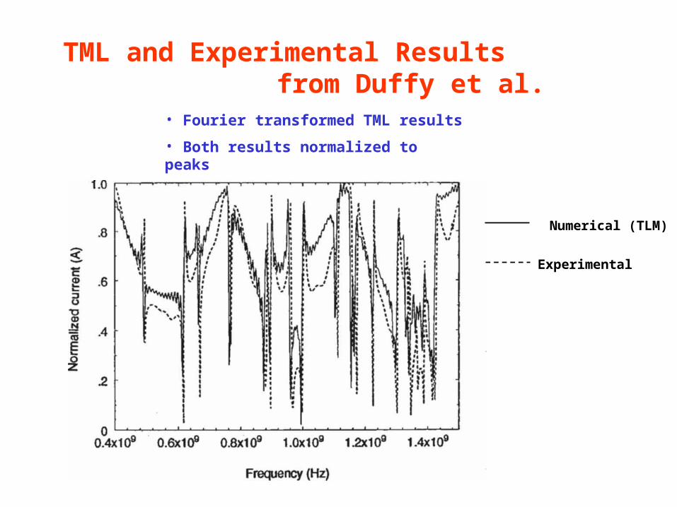
TML and Experimental Results from Duffy et al.
• Fourier transformed TML results
• Both results normalized to peaks
Numerical (TLM)
Experimental
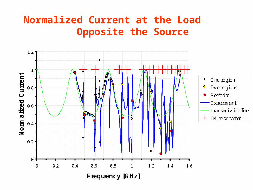
Normalized Current at the Load Opposite the Source
0
0.2
0.4
0.6
0.8
1
1.2
0 0.2 0.4 0.6 0.8 1 1.2 1.4 1.6
Frequency [GHz]
No
rma
lize
d C
urr
en
t
One region
Two regions
Periodic
Experiment
Transmission line
TM resonator

Detail of Current Plot (0.4 to 0.8 GHz)
0
0.2
0.4
0.6
0.8
1
1.2
0.4 0.6 0.8
Frequency [GHz]
No
rma
lize
d C
urr
ent One region
Two regions
Periodic
Experiment
Transmission line
TM resonator
Summary of EIGER Validation
• Consistent results are obtained utilizing three different formulations for a complex cavity/wire/aperture problem
• Results in agreement with independent experiments and calculations
• EIGER can be useful in EMC/EMI applications both as a stand-alone code and as a code validation tool
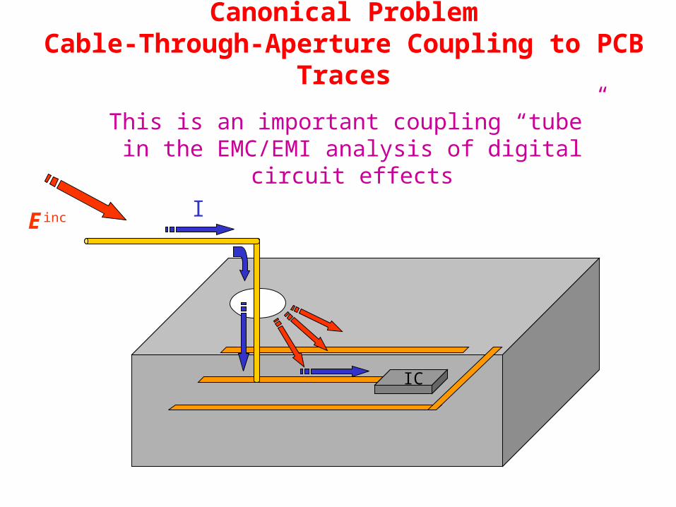
Canonical ProblemCable-Through-Aperture Coupling to PCB Traces
IC
E inc I
This is an important coupling “tube” in the EMC/EMI analysis of digital circuit effects

Canonical ProblemIssues, Goals, and Approaches
The cavity enclosure must be considered for an accurate solution.
The PCB trace may be very complicated, and on a very different size scale than the cavity.
Separate the cavity analysis from the PCB analysis to the maximum extent possible.
Issues:
Goal:

Calculate a Thévenin equivalent circuit at the input of the digital device (requires Voc and Isc).
Use transmission line theory (with distributed sources) to model the PCB trace.
Use EIGER to model the cable inside the cavity and the cavity fields, and combine this with the PCB transmission line modeling.
Approach
A hybrid method is developed that combines the rigorous cavity-field calculations of EIGER with transmission line theory.
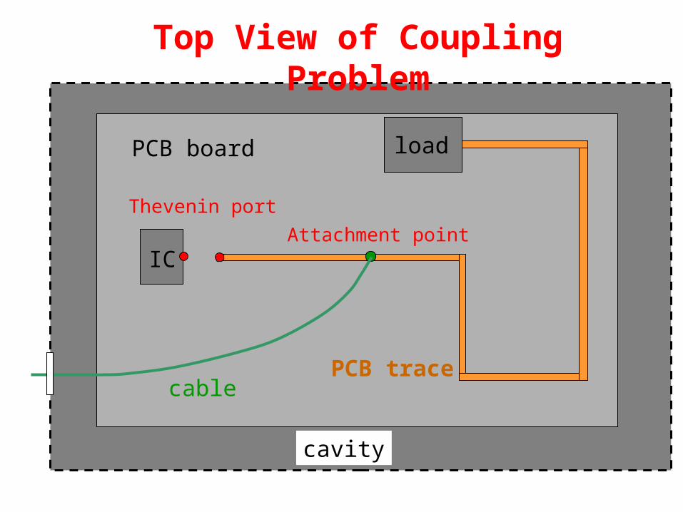
IC
Thevenin port
load
PCB trace
Attachment point
Top View of Coupling Problem
cavity
cable
PCB board
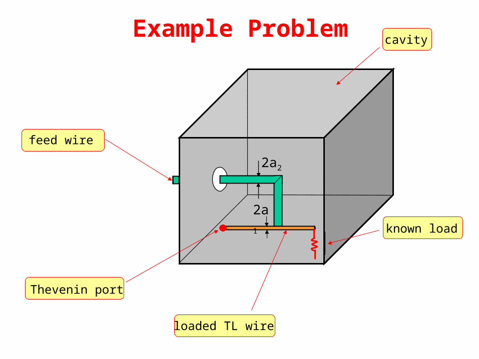
Example Problem
2a2
2a1
loaded TL wire
feed wire
Thevenin port
known load
cavity
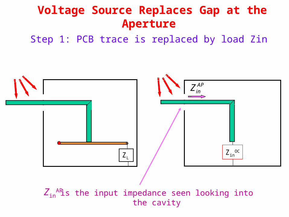
Voltage Source Replaces Gap at the Aperture
Step 1: PCB trace is replaced by load Zin
is the input impedance seen looking into the cavityZinAP
ZL
APinZ
ZinOC
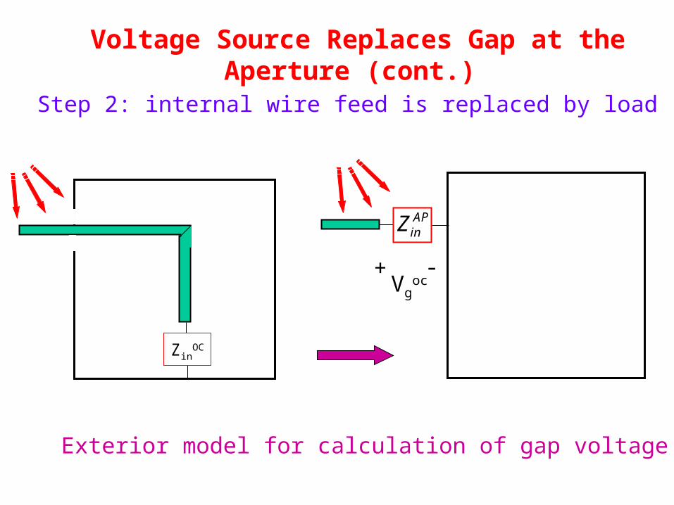
Voltage Source Replaces Gap at the Aperture (cont.)
Step 2: internal wire feed is replaced by load
Exterior model for calculation of gap voltage
APinZ
+ -Vg
oc
ZinOC

Voltage Source Replaces Gap at the Aperture (cont.)
ZL
- +
Voc
-
+
Vgoc

Current on the Wire is Calculated
The current on the feed wire and at the junction can be calculated by using EIGER.
ZinOC
- +
IJOC
I WOC
Vgoc
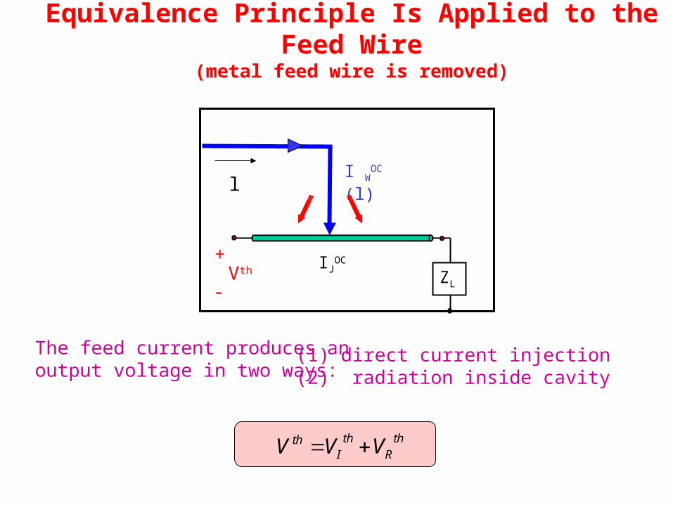
Equivalence Principle Is Applied to the Feed Wire(metal feed wire is removed)
The feed current produces an output voltage in two ways:
(1) direct current injection(2) radiation inside cavity
th ththI RV V V
ZLVth
+
-
I WOC (l)
IJOC
l
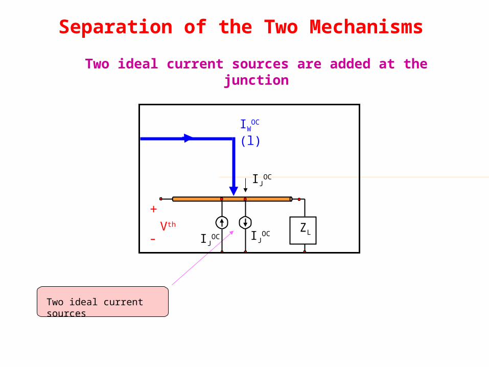
Separation of the Two Mechanisms
Two ideal current sources
Two ideal current sources are added at the junction
Vth
IJOC
IJOCIJ
OCZL
IWOC (l)
+
-

Mechanism 1: Injection Current
The “injected” Thevenin equivalent voltage comes from the ideal current source IJ
OC.
IJOC
VIth
ZL
2 1
+
-
Simple transmission line theory is used to calculate VIth

Mechanism 2: Radiation From Feed Wire
Radiation from feed wire creates a distributed voltage source along the PCB wire
VRth
IJOC
IJOC
ZL
I WOC (l)
2 1
+
-
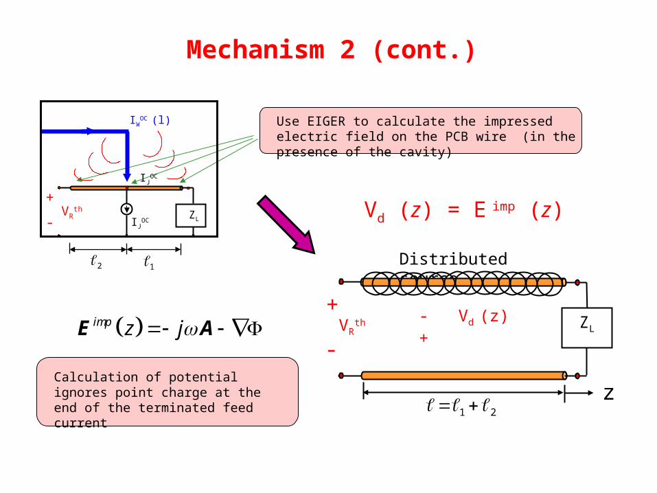
Mechanism 2 (cont.)
Use EIGER to calculate the impressed electric field on the PCB wire (in the presence of the cavity)
VRth
IWOC (l)
IJOC
IJOC
ZL
2 1
+
-
VRth
Distributed source
- Vd (z) + ZL
z1 2
+
-
Vd (z) = E imp (z)
imp z j E A
Calculation of potential ignores point charge at the end of the terminated feed current
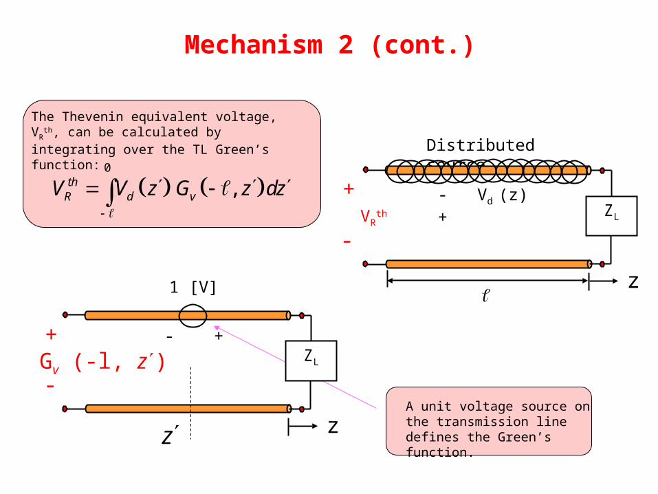
Mechanism 2 (cont.)
0
,thR d vV V z G z dz
The Thevenin equivalent voltage, VRth, can be
calculated by integrating over the TL Green’s function:
A unit voltage source on the transmission line defines the Green’s function.
VRth
Distributed source
- Vd (z) +ZL
z
+
-
- +ZL
z
1 [V]
z
Gv (-l, z)+
-
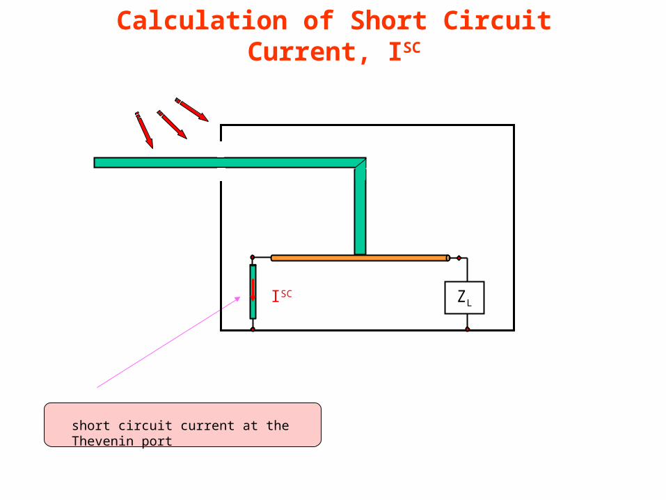
Calculation of Short Circuit Current, ISC
short circuit current at the Thevenin port
ISC ZL

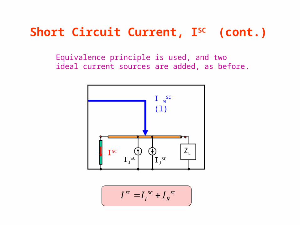
Short Circuit Current, ISC (cont.)
Procedure is similar to that used to obtain Thevenin (open-circuit) voltage:
Different terminating impedance results in a different gap voltage source
ZinSC
- +
IJSC
I WSC (l)
Vgsc
I WSC (l)
IJSCIJ
SC
ZLISC
Short Circuit Current, ISC (cont.)
Equivalence principle is used, and two ideal current sources are added, as before.
sc sc scI RI I I
IJSC
ZLI ISC
2 1
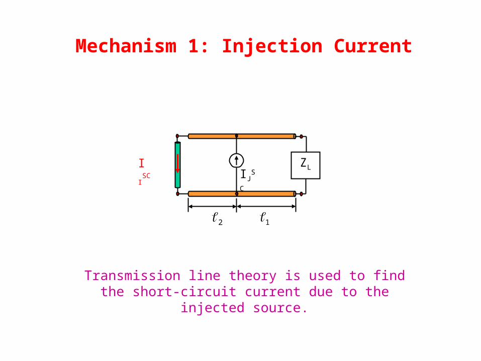
Mechanism 1: Injection Current
Transmission line theory is used to find the short-circuit current due to the injected source.
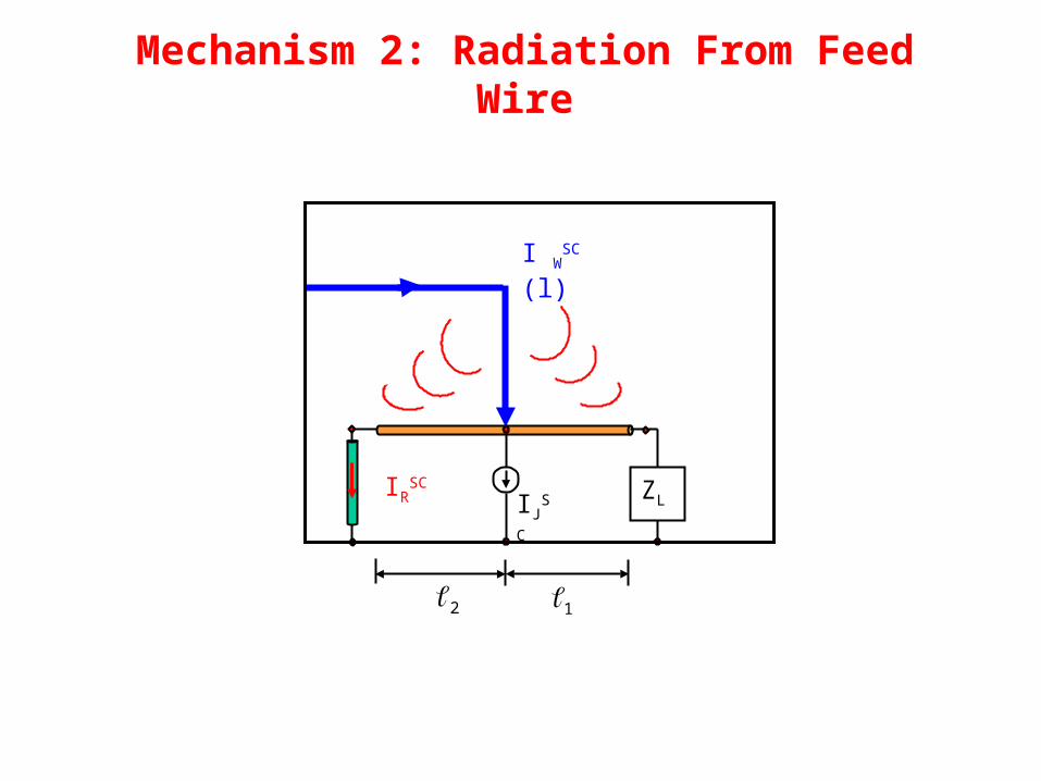
Mechanism 2: Radiation From Feed Wire
I WSC (l)
IJSC ZL
IRSC
2 1

Use EIGER to calculate impressed field on the PCB wire.
Distributed source
- Vd (z) +ZL
z1 2
IRSC
Mechanism 2 (cont.)
IWSC
IJSC ZLIR
SC
2 1
Calculation of potential ignores point charge at the end of the terminated feed current
imp z j E A
Vd (z) = E imp (z)
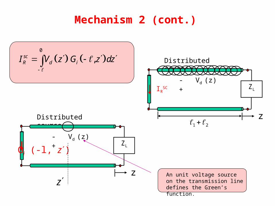
0
,scR d iI V z G z dz
An unit voltage source on the transmission line defines the Green’s function.
Distributed sources
- Vd (z) +ZL
z1 2
IRSC
Mechanism 2 (cont.)
Distributed source
- Vd (z) +ZL
zz
Gi (-l, z)

• Obtain numerical results using EIGER for example problem
• Validate approach by “brute force” comparison
Future Work


