
Outline DFT Action Dilute Renormalization Summary
Covariant Density Functional Theory
Dick Furnstahl
Department of PhysicsOhio State University
September, 2004
Collaborators: A. Bhattacharyya, J. Engel, H.-W. Hammer,J. Piekarewicz, S. Puglia, A. Schwenk, B. Serot
Dick Furnstahl Covariant DFT
Outline DFT Action Dilute Renormalization Summary
Covariant Density Functional Theory
Dick Furnstahl
Department of PhysicsOhio State University
September, 2004
Collaborators: A. Bhattacharyya, J. Engel, H.-W. Hammer,J. Piekarewicz, S. Puglia, A. Schwenk, B. Serot
Dick Furnstahl Covariant DFT

Outline DFT Action Dilute Renormalization Summary
5
82
50
28
28
50
82
2082
28
20
126
A=10
A=12 A~60
Density Functio
nal Theory
Selfconsis
tent Mean Field
Ab initiofew-body
calculations No-Core Shell Model G-matrix
r-process
rp-process
0Ñω ShellModel
Limits of nuclearexistence
pro
tons
neutrons
Many-body approachesfor ordinary nuclei
Figure 2: Top: the nuclear landscape - the territory of RIA physics. The black squares represent the stable nuclei and the nuclei with half-lives comparable to or longer than the age of the Earth (4.5 billion years). These nuclei form the "valley of stability". The yellow region indicates shorter lived nuclei that have been produced and studied in laboratories. By adding either protons or neutrons one moves away from the valley of stability, finally reaching the drip lines where the nuclear binding ends because the forces between neutrons and protons are no longer strong enough to hold these particles together. Many thousands of radioactive nuclei with very small or very large N/Z ratios are yet to be explored. In the (N,Z) landscape, they form the terra incognita indicated in green. The proton drip line is already relatively well delineated experimentally up to Z=83. In contrast, the neutron drip line is considerably further from the valley of stability and harder to approach. Except for the lightest nuclei where it has been reached experimentally, the neutron drip line has to be estimated on the basis of nuclear models - hence it is very uncertain due to the dramatic extrapolations involved. The red vertical and horizontal lines show the magic numbers around the valley of stability. The anticipated paths of astrophysical processes (r-process, purple line; rp-process, turquoise line) are shown. Bottom: various theoretical approaches to the nuclear many-body problem. For the lightest nuclei, ab initio calculations (Green’s Function Monte Carlo, no-core shell model) based on the bare nucleon-nucleon interaction, are possible. Medium-mass nuclei can be treated by the large-scale shell model. For heavy nuclei, the density functional theory (based on selfconsistent mean field) is the tool of choice. By investigating the intersections between these theoretical strategies, one aims at nothing less than developing the unified description of the nucleus.
Dick Furnstahl Covariant DFT

Outline DFT Action Dilute Renormalization Summary
Issues and Questions about Covariant DFT
How is covariant Kohn-Sham DFT more than Hartree?Where are the approximations?How do we include long-range effects?
What can you calculate in a DFT approach? Excited states?What about single-particle properties?
How do we carry out a covariant nuclear EFT and DFT?Functionals depending on just jµ or ρs also?Does point coupling vs. meson fields matter?What about “vacuum physics”?
How does pairing work in DFT? Does covariance matter?
Should we connect to the free NN interaction?What about chiral EFT or low-momentum interactions and RG?
Dick Furnstahl Covariant DFT

Outline DFT Action Dilute Renormalization Summary
Outline
(Relativistic) Kohn-Sham DFT
Effective Action Approach to EFT-Based Kohn-Sham DFT
Insights from Dilute Fermi Systems
Renormalization of Covariant Kohn-Sham DFT
Ongoing and Future Challenges
Dick Furnstahl Covariant DFT

Outline DFT Action Dilute Renormalization Summary Intro Covariant
Density Functional Theory (DFT)
Dominant application:inhomogeneouselectron gas
Interacting point electronsin static potential of atomicnuclei
“Ab initio” calculations ofatoms, molecules,crystals, surfaces
1970 1975 1980 1985 1990 199510
100
1000
year
num
ber
of r
etrie
ved
reco
rds
per
year
Density Functional Theory
Hartree−Fock
Dick Furnstahl Covariant DFT

Outline DFT Action Dilute Renormalization Summary Intro Covariant
Density Functional Theory (DFT)
Dominant application:inhomogeneouselectron gas
Interacting point electronsin static potential of atomicnuclei
“Ab initio” calculations ofatoms, molecules,crystals, surfaces
H2 C2 C2H2 CH4 C2H4 C2H6 C6H6
molecule
-100
-80
-60
-40
-20
0
20
% d
evia
tion
from
exp
erim
ent
Hartree-FockDFT Local Spin Density ApproximationDFT Generalized Gradient Approximation
Atomization Energies of Hydrocarbon Molecules
Dick Furnstahl Covariant DFT

Outline DFT Action Dilute Renormalization Summary Intro Covariant
Density Functional Theory (DFT)
Hohenberg-Kohn: There existsan energy functional Ev [ρ] . . .
Ev [ρ] = FHK [ρ] +
∫d3x v(x)ρ(x)
FHK is universal (same for anyexternal v ) =⇒ H2 to DNA!
Useful if you can approximatethe energy functional
Kohn-Sham procedure similarto nuclear “mean field”calculations
Dick Furnstahl Covariant DFT

Outline DFT Action Dilute Renormalization Summary Intro Covariant
Kohn-Sham DFT
VHO
=⇒VKS
Interacting density with vHO ≡ Non-interacting density with vKS
Orbitals φi(x) in local potential vKS([ρ], x) [but no M∗(x)]
[−∇2/2m + vKS(x)]φi = εiφi =⇒ ρ(x) =N∑
i=1
|φi(x)|2
Find Kohn-Sham potential vKS(x) from δEv [ρ]/δρ(x)Solve self-consistently
Dick Furnstahl Covariant DFT

Outline DFT Action Dilute Renormalization Summary Intro Covariant
Relativistic DFT
QED extension by Rajagopal/Callaway and Macdonald/VoskoSimilar HK theorems with jµ(x) instead of ρ(x)
and (four-vector) external potential
F [jµ] = E [jµ]−∫
d3x jµ(x)Vµext(x)
Kohn-Sham relativistic DFTSchrodinger equation −→ Dirac equation
Applications: materials containing heavy elements (Zα ∼ 1)Heavy-atom energies, magnetic moments of Fe, Co, Ni, . . .
QHD formulation by Speicher, Dreizler, and Engel (1992)
Questions and open problemsTreatment of UV divergences??? Vacuum subtractions???Construction of exchange-correlation functional (LDA?)
Dick Furnstahl Covariant DFT

Outline DFT Action Dilute Renormalization Summary Thermo Action KLW EFT
Thermodynamic Interpretation of DFT
Consider a system of spins Si
on a lattice with interaction g
The partition function has theinformation about the energy,magnetization of the system:
Z = Tr e−βg∑
i,j Si Sj
The magnetization M is
M =⟨∑
i
Si
⟩=
1Z
Tr
[(∑i
Si
)e−βg
∑i,j Si Sj
]
Dick Furnstahl Covariant DFT
Outline DFT Action Dilute Renormalization Summary Thermo Action KLW EFT
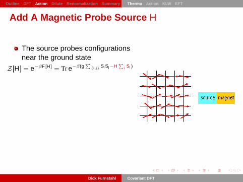
Add A Magnetic Probe Source H
The source probes configurationsnear the ground state
Z[H] = e−βF [H] = Tr e−β(g∑
i,j Si Sj−H∑
i Si )
Variations of the source yield themagnetization
M =⟨∑
i
Si
⟩H
= −∂F [H]
∂H
F [H] is the Helmholtz free energy.Set H = 0 (or equal to a realexternal source) at the end
Dick Furnstahl Covariant DFT

Outline DFT Action Dilute Renormalization Summary Thermo Action KLW EFT
Legendre Transformation to Effective Action
Find H[M] by inverting
M =⟨∑
i
Si
⟩H
= −∂F [H]
∂H
Legendre transform to the Gibbsfree energy
Γ[M] = F [H] + H M
The ground-state magnetizationMgs follows by minimizing Γ[M]:
H =∂Γ[M]
∂M−→ ∂Γ[M]
∂M
∣∣∣∣Mgs
= 0
Dick Furnstahl Covariant DFT

Outline DFT Action Dilute Renormalization Summary Thermo Action KLW EFT
Variational Energy and the Effective Action
Consider generalized Hamiltonian including time-independent H:
H(H) = g∑i,j
SiSj − H∑
i
Si
In the large β limit, Z =⇒ ground state of H(H) with energy
E(H) = limβ→∞
−1β
logZ
Separating out the pieces:
E(H) = 〈H(H)〉H = 〈H〉H − H⟨∑
i
Si
⟩H
= 〈H〉H − HM
Thus as T → 0, the effective action
Γ(M) = E(H) + HM = 〈H〉H
is the expectation value of H in the ground state generated by H
The true ground state (with H = 0) is the variational minimum!
Dick Furnstahl Covariant DFT

Outline DFT Action Dilute Renormalization Summary Thermo Action KLW EFT
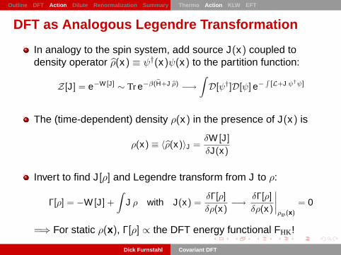
DFT as Analogous Legendre Transformation
In analogy to the spin system, add source J(x) coupled todensity operator ρ(x) ≡ ψ†(x)ψ(x) to the partition function:
Z[J] = e−W [J] ∼ Tr e−β(H+J ρ) −→∫D[ψ†]D[ψ] e−
∫[L+J ψ†ψ]
The (time-dependent) density ρ(x) in the presence of J(x) is
ρ(x) ≡ 〈ρ(x)〉J =δW [J]
δJ(x)
Invert to find J[ρ] and Legendre transform from J to ρ:
Γ[ρ] = −W [J] +
∫J ρ with J(x) =
δΓ[ρ]
δρ(x)−→ δΓ[ρ]
δρ(x)
∣∣∣∣ρgs(x)
= 0
=⇒ For static ρ(x), Γ[ρ] ∝ the DFT energy functional FHK !
Dick Furnstahl Covariant DFT

Outline DFT Action Dilute Renormalization Summary Thermo Action KLW EFT
DFT as Analogous Legendre Transformation
In analogy to the spin system, add source J(x) coupled todensity operator ρ(x) ≡ ψ†(x)ψ(x) to the partition function:
Z[J] = e−W [J] ∼ Tr e−β(H+J ρ) −→∫D[ψ†]D[ψ] e−
∫[L+J ψ†ψ]
The (time-dependent) density ρ(x) in the presence of J(x) is
ρ(x) ≡ 〈ρ(x)〉J =δW [J]
δJ(x)
Invert to find J[ρ] and Legendre transform from J to ρ:
Γ[ρ] = −W [J] +
∫J ρ with J(x) =
δΓ[ρ]
δρ(x)−→ δΓ[ρ]
δρ(x)
∣∣∣∣ρgs(x)
= 0
=⇒ For static ρ(x), Γ[ρ] ∝ the DFT energy functional FHK !
Dick Furnstahl Covariant DFT

Outline DFT Action Dilute Renormalization Summary Thermo Action KLW EFT
Covariant DFT as Legendre Transformation
In analogy to the spin system, add source V µ(x) coupled tocurrent operator jµ(x) ≡ ψ(x)γµψ(x) to the partition function:
Z[V ] = e−W [V ] ∼ Tr e−β(H+V ·j) −→∫D[ψ†]D[ψ] e−
∫[L+Vµ ψγ
µψ]
The (time-dependent) current jµ(x) in the presence of V µ(x) is
jµ(x) ≡ 〈jµ(x)〉V =δW [V ]
δvµ(x)
Invert to find V µ[j] and Legendre transform from V µ to jµ:
Γ[j] = −W [V ] +
∫v · j with Vµ(x) =
δΓ[j]δjµ(x)
−→ δΓ[j]δjµ(x)
∣∣∣∣jgs(x)
= 0
=⇒ For static jµ(x), Γ[j] ∝ the DFT energy functional FHK !
Dick Furnstahl Covariant DFT

Outline DFT Action Dilute Renormalization Summary Thermo Action KLW EFT
What About the Scalar Density?
Can add additional sources and Legendre transformations
In nonrelativistic DFT, add to Lagrangian + η(x) ∇ψ†∇ψ
Γ[ρ, τ ] = W [J, η]−∫
J(x)ρ(x)−∫η(x)τ(x)
=⇒ Skyrme HF energy functional E [ρ, τ, J] of densityand kinetic energy density
In covariant DFT, add to Lagrangian + S(x)ψψ
Γ[jµ, ρs] = W [Vµ,S]−∫
V (x) · j(x)−∫
S(x)ρs(x)
=⇒ RMF energy functional E [ρv , ρs] [with jµ = (ρv ,0)]
Dick Furnstahl Covariant DFT

Outline DFT Action Dilute Renormalization Summary Thermo Action KLW EFT
Possible Effective Actions
Couple source to local Lagrangian field, e.g., J(x)ϕ(x)
Γ[φ] where φ(x) = 〈ϕ(x)〉 =⇒ 1PI effective actionArises from fermion L’s by introducing auxiliary fields (mesons!)Kohn-Sham via special saddlepoint evaluation
Couple source to non-local composite op, e.g., J(x , x ′)ϕ(x)ϕ(x ′)
Γ[G, φ] =⇒ 2PI effective action [CJT]
Source coupled to local composite operator, e.g., J(x)ϕ2(x)
1.5PI effective action? Almost:Kohn-Sham from inversion method (point coupling!)Problem from new divergences =⇒ polynomial J(x) counterterms
“Sentenced to death” by Banks and Rabyenergy interpretation? variational?reprieve?
Dick Furnstahl Covariant DFT

Outline DFT Action Dilute Renormalization Summary Thermo Action KLW EFT
Kohn-Luttinger-Ward Theorem (1960)
T → 0 diagrammatic expansion of Ω(µ,V ,T ) in external v(x)=⇒ same as F (N,V ,T ≡ 0) with µ0 and no anomalous diagrams
Ω(µ, V, T ) = Ω0(µ) + + + + · · ·
with G0(µ, T )
T→0−→ F (N, V, T = 0) = E0(N) + + + · · ·
with G0(µ0)
Uniform Fermi system with no external potential (degeneracy ν):
µ0(N) = (6π2N/νV )2/3 ≡ k2F/2M ≡ ε0
F
If symmetry of non-interacting and interacting systems agree
Dick Furnstahl Covariant DFT

Outline DFT Action Dilute Renormalization Summary Thermo Action KLW EFT
Kohn-Luttinger Inversion Method [F & W, sec. 30]
Find F (N) = Ω(µ) + µN with µ(N) from N(µ) = −(∂Ω/∂µ)TV
expand about non-interacting system (subscripts label expansion):
Ω(µ) = Ω0(µ) + Ω1(µ) + Ω2(µ) + · · ·µ = µ0 + µ1 + µ2 + · · ·
F (N) = F0(N) + F1(N) + F2(N) + · · ·
invert N = −(∂Ω(µ)/∂µ)TV order-by-order in expansionN appears in 0th order only: N = −[∂Ω0/∂µ)]µ=µ0 =⇒ µ0(N)first order has two terms, which lets us solve for µ1:
0 = [∂Ω1/∂µ]µ=µ0 + µ1[∂2Ω0/∂µ
2]µ=µ0 =⇒ µ1 = − [∂Ω1/∂µ]µ=µ0
[∂2Ω0/∂µ2]µ=µ0
Same pattern to all orders: µi is determined by functions of µ0
Dick Furnstahl Covariant DFT

Outline DFT Action Dilute Renormalization Summary Thermo Action KLW EFT
Kohn-Luttinger Inversion Method [F & W, sec. 30]
Find F (N) = Ω(µ) + µN with µ(N) from N(µ) = −(∂Ω/∂µ)TV
expand about non-interacting system (subscripts label expansion):
Ω(µ) = Ω0(µ) + Ω1(µ) + Ω2(µ) + · · ·µ = µ0 + µ1 + µ2 + · · ·
F (N) = F0(N) + F1(N) + F2(N) + · · ·
invert N = −(∂Ω(µ)/∂µ)TV order-by-order in expansion
N appears in 0th order only: N = −[∂Ω0/∂µ)]µ=µ0 =⇒ µ0(N)first order has two terms, which lets us solve for µ1:
0 = [∂Ω1/∂µ]µ=µ0 + µ1[∂2Ω0/∂µ
2]µ=µ0 =⇒ µ1 = − [∂Ω1/∂µ]µ=µ0
[∂2Ω0/∂µ2]µ=µ0
Same pattern to all orders: µi is determined by functions of µ0
Dick Furnstahl Covariant DFT

Outline DFT Action Dilute Renormalization Summary Thermo Action KLW EFT
Kohn-Luttinger Inversion Method [F & W, sec. 30]
Find F (N) = Ω(µ) + µN with µ(N) from N(µ) = −(∂Ω/∂µ)TV
expand about non-interacting system (subscripts label expansion):
Ω(µ) = Ω0(µ) + Ω1(µ) + Ω2(µ) + · · ·µ = µ0 + µ1 + µ2 + · · ·
F (N) = F0(N) + F1(N) + F2(N) + · · ·
invert N = −(∂Ω(µ)/∂µ)TV order-by-order in expansionN appears in 0th order only: N = −[∂Ω0/∂µ)]µ=µ0 =⇒ µ0(N)
first order has two terms, which lets us solve for µ1:
0 = [∂Ω1/∂µ]µ=µ0 + µ1[∂2Ω0/∂µ
2]µ=µ0 =⇒ µ1 = − [∂Ω1/∂µ]µ=µ0
[∂2Ω0/∂µ2]µ=µ0
Same pattern to all orders: µi is determined by functions of µ0
Dick Furnstahl Covariant DFT

Outline DFT Action Dilute Renormalization Summary Thermo Action KLW EFT
Kohn-Luttinger Inversion Method [F & W, sec. 30]
Find F (N) = Ω(µ) + µN with µ(N) from N(µ) = −(∂Ω/∂µ)TV
expand about non-interacting system (subscripts label expansion):
Ω(µ) = Ω0(µ) + Ω1(µ) + Ω2(µ) + · · ·µ = µ0 + µ1 + µ2 + · · ·
F (N) = F0(N) + F1(N) + F2(N) + · · ·
invert N = −(∂Ω(µ)/∂µ)TV order-by-order in expansionN appears in 0th order only: N = −[∂Ω0/∂µ)]µ=µ0 =⇒ µ0(N)first order has two terms, which lets us solve for µ1:
0 = [∂Ω1/∂µ]µ=µ0 + µ1[∂2Ω0/∂µ
2]µ=µ0 =⇒ µ1 = − [∂Ω1/∂µ]µ=µ0
[∂2Ω0/∂µ2]µ=µ0
Same pattern to all orders: µi is determined by functions of µ0
Dick Furnstahl Covariant DFT

Outline DFT Action Dilute Renormalization Summary Thermo Action KLW EFT
Kohn-Luttinger Inversion Method [F & W, sec. 30]
Find F (N) = Ω(µ) + µN with µ(N) from N(µ) = −(∂Ω/∂µ)TV
expand about non-interacting system (subscripts label expansion):
Ω(µ) = Ω0(µ) + Ω1(µ) + Ω2(µ) + · · ·µ = µ0 + µ1 + µ2 + · · ·
F (N) = F0(N) + F1(N) + F2(N) + · · ·
invert N = −(∂Ω(µ)/∂µ)TV order-by-order in expansionN appears in 0th order only: N = −[∂Ω0/∂µ)]µ=µ0 =⇒ µ0(N)first order has two terms, which lets us solve for µ1:
0 = [∂Ω1/∂µ]µ=µ0 + µ1[∂2Ω0/∂µ
2]µ=µ0 =⇒ µ1 = − [∂Ω1/∂µ]µ=µ0
[∂2Ω0/∂µ2]µ=µ0
Same pattern to all orders: µi is determined by functions of µ0
Dick Furnstahl Covariant DFT

Outline DFT Action Dilute Renormalization Summary Thermo Action KLW EFT
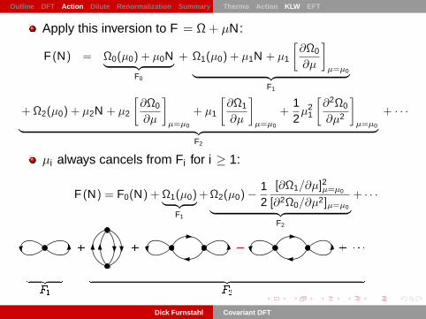
Apply this inversion to F = Ω + µN:
F (N) = Ω0(µ0) + µ0N︸ ︷︷ ︸F0
+ Ω1(µ0) + µ1N + µ1
[∂Ω0
∂µ
]µ=µ0︸ ︷︷ ︸
F1
+ Ω2(µ0) + µ2N + µ2
[∂Ω0
∂µ
]µ=µ0
+ µ1
[∂Ω1
∂µ
]µ=µ0
+12µ2
1
[∂2Ω0
∂µ2
]µ=µ0︸ ︷︷ ︸
F2
+ · · ·
µi always cancels from Fi for i ≥ 1:
F (N) = F0(N) + Ω1(µ0)︸ ︷︷ ︸F1
+Ω2(µ0)−12
[∂Ω1/∂µ]2µ=µ0
[∂2Ω0/∂µ2]µ=µ0︸ ︷︷ ︸F2
+ · · ·
Dick Furnstahl Covariant DFT

Outline DFT Action Dilute Renormalization Summary Thermo Action KLW EFT
Apply this inversion to F = Ω + µN:
F (N) = Ω0(µ0) + µ0N︸ ︷︷ ︸F0
+ Ω1(µ0) + µ1N + µ1
[∂Ω0
∂µ
]µ=µ0︸ ︷︷ ︸
F1
+ Ω2(µ0) + µ2N + µ2
[∂Ω0
∂µ
]µ=µ0
+ µ1
[∂Ω1
∂µ
]µ=µ0
+12µ2
1
[∂2Ω0
∂µ2
]µ=µ0︸ ︷︷ ︸
F2
+ · · ·
µi always cancels from Fi for i ≥ 1:
F (N) = F0(N) + Ω1(µ0)︸ ︷︷ ︸F1
+Ω2(µ0)−12
[∂Ω1/∂µ]2µ=µ0
[∂2Ω0/∂µ2]µ=µ0︸ ︷︷ ︸F2
+ · · ·
Dick Furnstahl Covariant DFT

Outline DFT Action Dilute Renormalization Summary Thermo Action KLW EFT
Generalizing the KLW Inversion Approach
Zeroth order is non-interacting system =⇒ easy to solveCommon feature of all generalizations =⇒ Kohn-Sham system!Here it has chemical potential µ0 and external potential v(x)
=⇒ fill levels up to µ0, which is known by counting up to N
But we still have a hard problem in finite systems
finding density ρ(x) in non-uniform system is complicated=⇒ it is not the density of the non-interacting system
for a self-bound system (nucleus!), there is no [net] v(x)
Introduce space-time dependent sourcesZeroth order system is always easy =⇒ single-particle orbitalsEnergy functional is very complicated before approximationNew feature: source −→ 0 in ground state (unlike µ)
Dick Furnstahl Covariant DFT

Outline DFT Action Dilute Renormalization Summary Thermo Action KLW EFT
Generalizing the KLW Inversion Approach
Zeroth order is non-interacting system =⇒ easy to solveCommon feature of all generalizations =⇒ Kohn-Sham system!Here it has chemical potential µ0 and external potential v(x)
=⇒ fill levels up to µ0, which is known by counting up to N
But we still have a hard problem in finite systemsfinding density ρ(x) in non-uniform system is complicated
=⇒ it is not the density of the non-interacting systemfor a self-bound system (nucleus!), there is no [net] v(x)
Introduce space-time dependent sourcesZeroth order system is always easy =⇒ single-particle orbitalsEnergy functional is very complicated before approximationNew feature: source −→ 0 in ground state (unlike µ)
Dick Furnstahl Covariant DFT

Outline DFT Action Dilute Renormalization Summary Thermo Action KLW EFT
Generalizing the KLW Inversion Approach
Three generalizations: Kohn-Sham DFT, other sources, pairing1. µN + J(x)ρ(x) with J(x) = δF [ρ]/δρ(x) → 0 in gs
2. Add a source coupled to the kinetic energy density
+ η(x)τ(x) where τ(x) ≡ 〈∇ψ† ·∇ψ〉
=⇒ M∗(x) in the Kohn-Sham equation (cf. Skyrme)
[−∇2
2M+ vKS(x)
]ψα = εαψα =⇒
[−∇ 1
M∗(x)∇ + vKS(x)
]ψα = εαψα
3. Add a source coupled to the divergent pair density=⇒ e.g., j〈ψ†
↑ψ†↓ + ψ↓ψ↑〉 =⇒ set j to zero in gs
Same inversion method, but use [J]gs = J0 + J1 + J2 + · · · = 0=⇒ solve for J0 iteratively: [J0]old =⇒ [J0]new = −J1 − J2 + · · ·
Dick Furnstahl Covariant DFT

Outline DFT Action Dilute Renormalization Summary Thermo Action KLW EFT
Generalizing the KLW Inversion Approach
Three generalizations: Kohn-Sham DFT, other sources, pairing1. µN + J(x)ρ(x) with J(x) = δF [ρ]/δρ(x) → 0 in gs2. Add a source coupled to the kinetic energy density
+ η(x)τ(x) where τ(x) ≡ 〈∇ψ† ·∇ψ〉
=⇒ M∗(x) in the Kohn-Sham equation (cf. Skyrme)
[−∇2
2M+ vKS(x)
]ψα = εαψα =⇒
[−∇ 1
M∗(x)∇ + vKS(x)
]ψα = εαψα
3. Add a source coupled to the divergent pair density=⇒ e.g., j〈ψ†
↑ψ†↓ + ψ↓ψ↑〉 =⇒ set j to zero in gs
Same inversion method, but use [J]gs = J0 + J1 + J2 + · · · = 0=⇒ solve for J0 iteratively: [J0]old =⇒ [J0]new = −J1 − J2 + · · ·
Dick Furnstahl Covariant DFT

Outline DFT Action Dilute Renormalization Summary Thermo Action KLW EFT
Generalizing the KLW Inversion Approach
Three generalizations: Kohn-Sham DFT, other sources, pairing1. µN + V µ(x)jµ(x) with V µ(x) = δF [j]/δµ(x) → 0 in gs2. Add a source coupled to the scalar density
+ S(x)ρs(x) where S(x) ≡ 〈ψψ〉
=⇒ M∗(x) = M − S0(x) in the Kohn-Sham Dirac equation[−iα·∇+βM+W0(x)
]ψα = εαψα =⇒
[−iα·∇+βM∗(x)+W0(x)
]ψα = εαψα
3. Add a source coupled to the divergent pair density=⇒ e.g., j〈ψTηψ〉 =⇒ set j to zero in gs
Same inversion method, but use [S]gs = S0 + S1 + S2 + · · · = 0=⇒ solve for S0 iteratively: [S0]old =⇒ [S0]new = −S1−S2 + · · ·
Dick Furnstahl Covariant DFT

Outline DFT Action Dilute Renormalization Summary Thermo Action KLW EFT
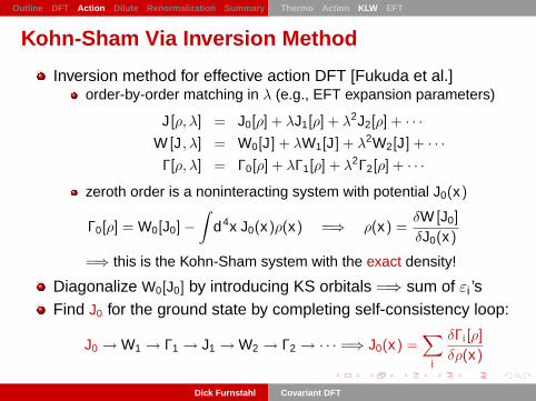
Kohn-Sham Via Inversion Method
Inversion method for effective action DFT [Fukuda et al.]order-by-order matching in λ (e.g., EFT expansion parameters)
J[ρ, λ] = J0[ρ] + λJ1[ρ] + λ2J2[ρ] + · · ·W [J, λ] = W0[J] + λW1[J] + λ2W2[J] + · · ·Γ[ρ, λ] = Γ0[ρ] + λΓ1[ρ] + λ2Γ2[ρ] + · · ·
zeroth order is a noninteracting system with potential J0(x)
Γ0[ρ] = W0[J0]−∫
d4x J0(x)ρ(x) =⇒ ρ(x) =δW [J0]
δJ0(x)
=⇒ this is the Kohn-Sham system with the exact density!
Diagonalize W0[J0] by introducing KS orbitals =⇒ sum of εi ’sFind J0 for the ground state by completing self-consistency loop:
J0 → W1 → Γ1 → J1 → W2 → Γ2 → · · · =⇒ J0(x) =∑
i
δΓi [ρ]
δρ(x)
Dick Furnstahl Covariant DFT

Outline DFT Action Dilute Renormalization Summary Thermo Action KLW EFT
Kohn-Sham Via Inversion Method
Inversion method for effective action DFT [Fukuda et al.]order-by-order matching in λ (e.g., EFT expansion parameters)
J[ρ, λ] = J0[ρ] + λJ1[ρ] + λ2J2[ρ] + · · ·W [J, λ] = W0[J] + λW1[J] + λ2W2[J] + · · ·Γ[ρ, λ] = Γ0[ρ] + λΓ1[ρ] + λ2Γ2[ρ] + · · ·
zeroth order is a noninteracting system with potential J0(x)
Γ0[ρ] = W0[J0]−∫
d4x J0(x)ρ(x) =⇒ ρ(x) =δW [J0]
δJ0(x)
=⇒ this is the Kohn-Sham system with the exact density!
Diagonalize W0[J0] by introducing KS orbitals =⇒ sum of εi ’s
Find J0 for the ground state by completing self-consistency loop:
J0 → W1 → Γ1 → J1 → W2 → Γ2 → · · · =⇒ J0(x) =∑
i
δΓi [ρ]
δρ(x)
Dick Furnstahl Covariant DFT
Outline DFT Action Dilute Renormalization Summary Thermo Action KLW EFT
Kohn-Sham Via Inversion Method
Inversion method for effective action DFT [Fukuda et al.]order-by-order matching in λ (e.g., EFT expansion parameters)
J[ρ, λ] = J0[ρ] + λJ1[ρ] + λ2J2[ρ] + · · ·W [J, λ] = W0[J] + λW1[J] + λ2W2[J] + · · ·Γ[ρ, λ] = Γ0[ρ] + λΓ1[ρ] + λ2Γ2[ρ] + · · ·
zeroth order is a noninteracting system with potential J0(x)
Γ0[ρ] = W0[J0]−∫
d4x J0(x)ρ(x) =⇒ ρ(x) =δW [J0]
δJ0(x)
=⇒ this is the Kohn-Sham system with the exact density!
Diagonalize W0[J0] by introducing KS orbitals =⇒ sum of εi ’sFind J0 for the ground state by completing self-consistency loop:
J0 → W1 → Γ1 → J1 → W2 → Γ2 → · · · =⇒ J0(x) =∑
i
δΓi [ρ]
δρ(x)
Dick Furnstahl Covariant DFT

Outline DFT Action Dilute Renormalization Summary Thermo Action KLW EFT
Why Use EFT for Energy Functionals
Similar to conventional “phenomenological” approachesbut with a rigorous foundation (DFT from effective action)extendable and can be connected to chiral EFT
or vlow k for NN and few-body
Eliminating model dependences (cf. “minimal” models!)framework for building a “complete” functionalmore efficient renormalization
New insight into analytic structure of functionale.g., logs in low-density expansion in kFas from RG
Power counting: what to sum at each order in an expansionnaturalness =⇒ estimates of truncation errorsevidence from Skyrme and RMF functionals for hierarchyfor covariant EFT, requires special renormalization
Dick Furnstahl Covariant DFT

Outline DFT Action Dilute Renormalization Summary DFT/EFT Results Tau M∗ Pairing
“Simple” Many-Body Problem: Hard Spheres
Infinite potential at radius R
0 R
sin(kr+δ)
r
Scattering length a0 = R
Dilute nR3 1 =⇒ kFa0 1
What is the energy / particle?
k F
R
1/~
Dick Furnstahl Covariant DFT

Outline DFT Action Dilute Renormalization Summary DFT/EFT Results Tau M∗ Pairing
In Search of a Perturbative Expansion
For free-space scattering at momentum k 1/R, we shouldrecover a perturbative expansion in kR for scattering amplitude:
f0(k) ∝ 1k cot δ(k)− ik
−→ a0 − ia20k − (a3
0 − a20r0/2)k2 +O(k3a3
0)
with a0 = R and r0 = 2R/3 for hard-core spheres
Perturbation theory in the hard-core potential won’t work:
0 R
=⇒ 〈k|V |k′〉 ∝∫
dx eik·x V (x) e−ik′·x −→∞
Standard solution: Solve nonperturbatively, then expand
EFT approach: k 1/R means we probe at low resolution=⇒ replace potential with a simpler but general interaction
Dick Furnstahl Covariant DFT

Outline DFT Action Dilute Renormalization Summary DFT/EFT Results Tau M∗ Pairing
Nonrelativistic EFT for “Natural” Dilute Fermions
A simple, general interaction is a sum of delta functions andderivatives of delta functions. In momentum space (cf. Skyrme),
〈k|Veft|k′〉 = C0 +12
C2(k2 + k′2) + C′2k · k′ + · · ·
Or, Left has most general local (contact) interactions:
Left = ψ†[i∂
∂t+
−→∇ 2
2M
]ψ − C0
2(ψ†ψ)2 +
C2
16
[(ψψ)†(ψ
↔∇2ψ) + h.c.
]+
C′2
8(ψ
↔∇ψ)† · (ψ
↔∇ψ)− D0
6(ψ†ψ)3 + . . .
Dimensional analysis =⇒ C2i ∼ 4πM R2i+1 , D2i ∼ 4π
M R2i+4
Dick Furnstahl Covariant DFT

Outline DFT Action Dilute Renormalization Summary DFT/EFT Results Tau M∗ Pairing
Renormalization
Reproduce: f0(k) ∝ a0 − ia20k − (a3
0 − a20r0/2)k2 +O(k3a3
0)
Consider the leading potential V (0)EFT(x) = C0δ(x) or
〈k|V (0)eft |k
′〉 =⇒ =⇒ C0
Choosing C0 ∝ a0 gets the first term. Now 〈k|VG0V |k′〉:
=⇒∫
d3q(2π)3
1k2 − q2 + iε
−→∞!
=⇒ Linear divergence!
Dick Furnstahl Covariant DFT

Outline DFT Action Dilute Renormalization Summary DFT/EFT Results Tau M∗ Pairing
Renormalization
Reproduce: f0(k) ∝ a0 − ia20k − (a3
0 − a20r0/2)k2 +O(k3a3
0)
Consider the leading potential V (0)EFT(x) = C0δ(x) or
〈k|V (0)eft |k
′〉 =⇒ =⇒ C0
Choosing C0 ∝ a0 gets the first term. Now 〈k|VG0V |k′〉:
=⇒∫ Λc d3q
(2π)3
1k2 − q2 + iε
−→ Λc
2π2 −ik4π
+O(k2/Λc)
=⇒ If cutoff at Λc , then can absorb into V (0), but all powers of k2
Dick Furnstahl Covariant DFT
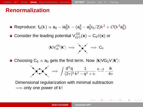
Outline DFT Action Dilute Renormalization Summary DFT/EFT Results Tau M∗ Pairing
Renormalization
Reproduce: f0(k) ∝ a0 − ia20k − (a3
0 − a20r0/2)k2 +O(k3a3
0)
Consider the leading potential V (0)EFT(x) = C0δ(x) or
〈k|V (0)eft |k
′〉 =⇒ =⇒ C0
Choosing C0 ∝ a0 gets the first term. Now 〈k|VG0V |k′〉:
=⇒∫
dDq(2π)3
1k2 − q2 + iε
D→3−→ − ik4π
Dimensional regularization with minimal subtraction=⇒ only one power of k !
Dick Furnstahl Covariant DFT

Outline DFT Action Dilute Renormalization Summary DFT/EFT Results Tau M∗ Pairing
Dim. reg. + minimal subtraction =⇒ simple power counting:
P/2− k
P/2 + k
P/2− k′
P/2 + k′
= +
iT (k, cos θ) − iC0 − M
4π(C0)
2k
+ + + + O(k3)
+i
(M
4π
)2
(C0)3k2 − iC2k
2 − iC ′2k2 cos θ
Matching: C0 = 4πM a0 = 4π
M R , C2 = 4πM
a20r02 = 4π
MR3
3 , · · ·
Recovers effective range expansion order-by-order withperturbative diagrammatic expansion
one power of k per diagramestimate truncation error from dimensional analysis
Dick Furnstahl Covariant DFT

Outline DFT Action Dilute Renormalization Summary DFT/EFT Results Tau M∗ Pairing
Now Sum Over Fermions in the Fermi Sea
Leading order V (0)EFT(x) = C0δ(x)
=⇒ ∝ a0k6F
At the next order, we get a linear divergence again:
=⇒ ∝∫ ∞
kF
d3q(2π)3
1k2 − q2
Same renormalization fixes it! Particles −→ holes∫ ∞
kF
1k2 − q2 =
∫ ∞
0
1k2 − q2−
∫ kF
0
1k2 − q2
D→3−→ −∫ kF
0
1k2 − q2 ∝ a2
0k7F
Dick Furnstahl Covariant DFT
Outline DFT Action Dilute Renormalization Summary DFT/EFT Results Tau M∗ Pairing
T = 0 Energy Density from Hugenholtz Diagrams
Dick Furnstahl Covariant DFT

Outline DFT Action Dilute Renormalization Summary DFT/EFT Results Tau M∗ Pairing
T = 0 Energy Density from Hugenholtz Diagrams
O(k6
F
):
O(k7
F
): +
O(k8
F
): +
+ +
+
EV
= ρk2
F
2M
[35
+ (ν − 1)2
3π(kFa0)
+ (ν − 1)4
35π2 (11− 2 ln 2)(kFa0)2
+ (ν − 1)(0.076 + 0.057(ν − 3)
)(kFa0)
3
+ (ν − 1)1
10π(kFr0)(kFa0)
2
+ (ν + 1)1
5π(kFap)
3 + · · ·
]
Dick Furnstahl Covariant DFT

Outline DFT Action Dilute Renormalization Summary DFT/EFT Results Tau M∗ Pairing
T = 0 Energy Density from Hugenholtz Diagrams
O(k6
F
):
O(k7
F
): +
O(k8
F
): +
+ +
+
EV
= ρk2
F
2M
[35
+ (ν − 1)2
3π(kFa0)
+ (ν − 1)4
35π2 (11− 2 ln 2)(kFa0)2
+ (ν − 1)(0.076 + 0.057(ν − 3)
)(kFa0)
3
+ (ν − 1)1
10π(kFr0)(kFa0)
2
+ (ν + 1)1
5π(kFap)
3 + · · ·]
Dick Furnstahl Covariant DFT

Outline DFT Action Dilute Renormalization Summary DFT/EFT Results Tau M∗ Pairing
T = 0 Energy Density from Hugenholtz Diagrams
LO :
NLO : +
NNLO : +
+ +
+
E =
∫d3x
[K (x) +
12
(ν − 1)
ν
4πa0
M[ρ(x)]2
+ d1a2
0
2M[ρ(x)]7/3
+ d2 a30[ρ(x)]8/3
+ d3 a20 r0[ρ(x)]8/3
+ d4 a3p[ρ(x)]8/3 + · · ·
]
Dick Furnstahl Covariant DFT

Outline DFT Action Dilute Renormalization Summary DFT/EFT Results Tau M∗ Pairing
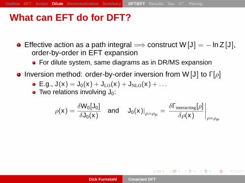
What can EFT do for DFT?
Effective action as a path integral =⇒ construct W [J] = − ln Z [J],order-by-order in EFT expansion
For dilute system, same diagrams as in DR/MS expansion
Inversion method: order-by-order inversion from W [J] to Γ[ρ]
E.g., J(x) = J0(x) + JLO(x) + JNLO(x) + . . .Two relations involving J0:
ρ(x) =δW0[J0]
δJ0(x)and J0(x)|ρ=ρgs
=δΓinteracting[ρ]
δρ(x)
∣∣∣∣ρ=ρgs
Interpretation: J0 is the external potential that yields for anoninteracting system the exact density
This is the Kohn-Sham potential!Two conditions on J0 =⇒ Self-consistency
Dick Furnstahl Covariant DFT
Outline DFT Action Dilute Renormalization Summary DFT/EFT Results Tau M∗ Pairing
What can EFT do for DFT?
Effective action as a path integral =⇒ construct W [J] = − ln Z [J],order-by-order in EFT expansion
For dilute system, same diagrams as in DR/MS expansion
Inversion method: order-by-order inversion from W [J] to Γ[ρ]
E.g., J(x) = J0(x) + JLO(x) + JNLO(x) + . . .Two relations involving J0:
ρ(x) =δW0[J0]
δJ0(x)and J0(x)|ρ=ρgs
=δΓinteracting[ρ]
δρ(x)
∣∣∣∣ρ=ρgs
Interpretation: J0 is the external potential that yields for anoninteracting system the exact density
This is the Kohn-Sham potential!Two conditions on J0 =⇒ Self-consistency
Dick Furnstahl Covariant DFT
Outline DFT Action Dilute Renormalization Summary DFT/EFT Results Tau M∗ Pairing
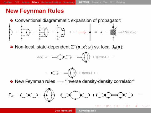
New Feynman Rules
Conventional diagrammatic expansion of propagator:
+ + + + · · · =⇒ = +x′
x=⇒ Σ∗(x,x′;ω)
Non-local, state-dependent Σ∗(x, x′;ω) vs. local J0(x):
J0(x) = − − + (perms.) + · · ·
= − + (perms.) + · · ·
New Feynman rules =⇒ “inverse density-density correlator”
Dick Furnstahl Covariant DFT

Outline DFT Action Dilute Renormalization Summary DFT/EFT Results Tau M∗ Pairing
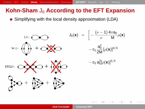
Kohn-Sham J0 According to the EFT ExpansionSimplifying with the local density approximation (LDA)
LO :
+ +
+
J0(x) =
[
− (ν − 1)
ν
4πa0
Mρ(x)
− c1a2
0
2M[ρ(x)]4/3
− c2 a30[ρ(x)]5/3
− c3 a20 r0[ρ(x)]5/3
− c4 a3p[ρ(x)]5/3 + · · ·
]
Dick Furnstahl Covariant DFT

Outline DFT Action Dilute Renormalization Summary DFT/EFT Results Tau M∗ Pairing
Kohn-Sham J0 According to the EFT ExpansionSimplifying with the local density approximation (LDA)
LO :
+ +
+
J0(x) =
[− (ν − 1)
ν
4πa0
Mρ(x)
− c1a2
0
2M[ρ(x)]4/3
− c2 a30[ρ(x)]5/3
− c3 a20 r0[ρ(x)]5/3
− c4 a3p[ρ(x)]5/3 + · · ·
]
Dick Furnstahl Covariant DFT
Outline DFT Action Dilute Renormalization Summary DFT/EFT Results Tau M∗ Pairing
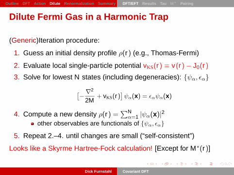
Dilute Fermi Gas in a Harmonic Trap
(Generic)Iteration procedure:
1. Guess an initial density profile ρ(r) (e.g., Thomas-Fermi)
2. Evaluate local single-particle potential vKS(r) ≡ v(r)− J0(r)
3. Solve for lowest N states (including degeneracies): ψα, εα
[−∇
2
2M+ vKS(r)
]ψα(x) = εαψα(x)
4. Compute a new density ρ(r) =∑N
α=1 |ψα(x)|2other observables are functionals of ψα, εα
5. Repeat 2.–4. until changes are small (“self-consistent”)
Looks like a Skyrme Hartree-Fock calculation! [Except for M∗(r)]
Dick Furnstahl Covariant DFT

Outline DFT Action Dilute Renormalization Summary DFT/EFT Results Tau M∗ Pairing
Dilute Fermi Gas in a Harmonic Trap
(Generic)Iteration procedure:
1. Guess an initial density profile ρ(r) (e.g., Thomas-Fermi)
2. Evaluate local single-particle potential vKS(r) ≡ v(r)− J0(r)
3. Solve for lowest N states (including degeneracies): ψα, εα
[−∇
2
2M+ vKS(r)
]ψα(x) = εαψα(x)
4. Compute a new density ρ(r) =∑N
α=1 |ψα(x)|2other observables are functionals of ψα, εα
5. Repeat 2.–4. until changes are small (“self-consistent”)
Looks like a Skyrme Hartree-Fock calculation! [Except for M∗(r)]
Dick Furnstahl Covariant DFT

Outline DFT Action Dilute Renormalization Summary DFT/EFT Results Tau M∗ Pairing
Check Out An Example
0 1 2 3 4 5r/b
0
1
2
3
4ρ(
r/b)
C0 = 0 (exact)
Dilute Fermi Gas in Harmonic TrapNF=7, A=240, g=2, as=-0.160
E/A <kFas> <r2>1/2
6.750 -0.524 2.598
Dick Furnstahl Covariant DFT

Outline DFT Action Dilute Renormalization Summary DFT/EFT Results Tau M∗ Pairing
Check Out An Example
0 1 2 3 4 5r/b
0
1
2
3
4ρ(
r/b)
C0 = 0 (exact)Kohn-Sham LO
Dilute Fermi Gas in Harmonic TrapNF=7, A=240, g=2, as=-0.160
E/A <kFas> <r2>1/2
6.750 -0.524 2.598 5.982 -0.578 2.351
Dick Furnstahl Covariant DFT

Outline DFT Action Dilute Renormalization Summary DFT/EFT Results Tau M∗ Pairing
Check Out An Example
0 1 2 3 4 5r/b
0
1
2
3
4ρ(
r/b)
C0 = 0 (exact)Kohn-Sham LOKohn-Sham NLO (LDA)
Dilute Fermi Gas in Harmonic TrapNF=7, A=240, g=2, as=-0.160
E/A <kFas> <r2>1/2
6.750 -0.524 2.598 5.982 -0.578 2.351 6.254 -0.550 2.472
Dick Furnstahl Covariant DFT

Outline DFT Action Dilute Renormalization Summary DFT/EFT Results Tau M∗ Pairing
Check Out An Example
0 1 2 3 4 5r/b
0
1
2
3
4ρ(
r/b)
C0 = 0 (exact)Kohn-Sham LOKohn-Sham NLO (LDA)Kohn-Sham NNLO (LDA)
Dilute Fermi Gas in Harmonic TrapNF=7, A=240, g=2, as=-0.160
E/A <kFas> <r2>1/2
6.750 -0.524 2.598 5.982 -0.578 2.351 6.254 -0.550 2.472 6.227 -0.553 2.459
Dick Furnstahl Covariant DFT
Outline DFT Action Dilute Renormalization Summary DFT/EFT Results Tau M∗ Pairing
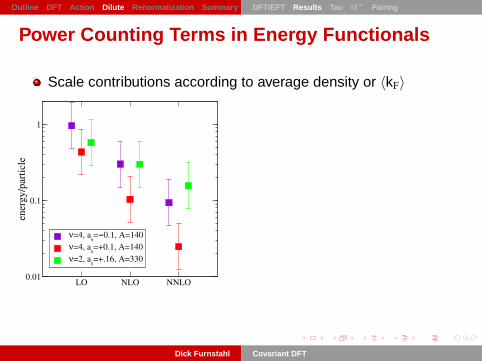
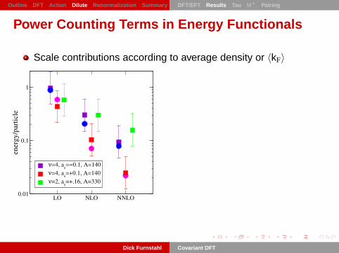
Power Counting Terms in Energy Functionals
Scale contributions according to average density or 〈kF〉
LO NLO NNLO0.01
0.1
1
ener
gy/p
artic
le
ν=4, as=-0.1, A=140ν=4, as=+0.1, A=140ν=2, as=+.16, A=330
Reasonable estimates =⇒ truncation errors understood
Dick Furnstahl Covariant DFT

Outline DFT Action Dilute Renormalization Summary DFT/EFT Results Tau M∗ Pairing
Power Counting Terms in Energy Functionals
Scale contributions according to average density or 〈kF〉
LO NLO NNLO0.01
0.1
1
ener
gy/p
artic
le
ν=4, as=-0.1, A=140ν=4, as=+0.1, A=140ν=2, as=+.16, A=330
Reasonable estimates =⇒ truncation errors understood
Dick Furnstahl Covariant DFT

Outline DFT Action Dilute Renormalization Summary DFT/EFT Results Tau M∗ Pairing
Beyond Kohn-Sham LDA: Kinetic Energy Density
Coulomb meta-GGA DFT uses E [ρ, τ(ρ)], with τ ≡ 〈∇ψ† ·∇ψ〉But τ is expanded in terms of ρ
τ(x) =35
(3π2)2/3 ρ5/3 +1
36(∇ρ)2
ρ+ · · ·
=⇒ same Kohn-Sham equation
J0(x) =δEint[ρ]
δρ(x)=⇒
[−∇2
2M+ J0(x)
]ψα = εαψα
In Skyrme HF, ρ and τ are treated independently in E [ρ, τ, J]
E [ρ, τ, J] =
∫d3x
1
2Mτ +
38
t0ρ2 +1
16t3ρ2+α +
116
(3t1 + 5t2)ρτ
+1
64(9t1 − 5t2)(∇ρ)2 − 3
4W0ρ∇ · J +
132
(t1 − t2)J2
Dick Furnstahl Covariant DFT

Outline DFT Action Dilute Renormalization Summary DFT/EFT Results Tau M∗ Pairing
To do this in DFT/EFT, add to Lagrangian + η(x) ∇ψ†∇ψ
Γ[ρ, τ ] = W [J, η]−∫
J(x)ρ(x)−∫η(x)τ(x)
Two Kohn-Sham potentials:
J0(x) =δEint[ρ, τ ]
δρ(x)and η0(x) =
δEint[ρ, τ ]
δτ(x)
Quadratic part of Lagrangian in W0 diagonalized:∫d4x ψ†
[i∂t +
∇ 2
2M− v(x) + J0(x)−∇ · η0(x)∇
]ψ
Kohn-Sham equation =⇒ defines 1/2M∗(x) ≡ 1/2M − η0(x)
Dick Furnstahl Covariant DFT
Outline DFT Action Dilute Renormalization Summary DFT/EFT Results Tau M∗ Pairing
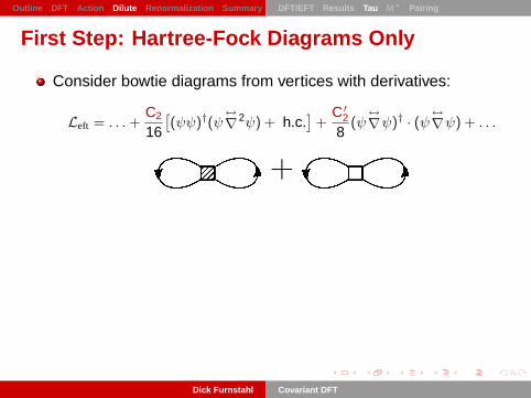
First Step: Hartree-Fock Diagrams Only
Consider bowtie diagrams from vertices with derivatives:
Left = . . .+C2
16
[(ψψ)†(ψ
↔∇2ψ) + h.c.
]+
C′2
8(ψ
↔∇ψ)† · (ψ
↔∇ψ) + . . .
+
Energy density in Kohn-Sham LDA (ν = 2):
Eint[ρ] = . . .+C2
8
[35
(6π2
ν
)2/3
ρ8/3]
+3C′
2
8
[35
(6π2
ν
)2/3
ρ8/3]
+ . . .
Energy density in Kohn-Sham with τ (ν = 2):
Eint[ρ, τ ] = . . .+C2
8
[ρτ +
34
(∇ρ)2]+3C′
2
8
[ρτ − 1
4(∇ρ)2]+ . . .
Dick Furnstahl Covariant DFT

Outline DFT Action Dilute Renormalization Summary DFT/EFT Results Tau M∗ Pairing
Power Counting Estimates Work for Gradients!
LO NLO LDA ρτ 10*∇ρ
0.01
0.1
1
ener
gy/p
artic
le
ap = as
ap=0
ν =2, as = 0.16, A = 240
τ -NNLO
LO NLO LDA ρτ 10*(∇ρ)0.001
0.01
0.1
1
ener
gy/p
artic
le
ap = as
ap=0
ν =4, as = 0.10, A = 140
τ -NNLO
Dick Furnstahl Covariant DFT

Outline DFT Action Dilute Renormalization Summary DFT/EFT Results Tau M∗ Pairing
Kohn-Sham LDA ρ vs. ρτ [Anirban Bhattacharyya]
0 1 2 3 4 5r/b
0
0.5
1
1.5
2ρ(
r/b)
ρ-DFT, ap = as
ρτ-DFT, ap = as
ρ-DFT, ap = 2as
ρτ-DFT, ap = 2 as
ν=2, NF=7, A=240as=0.16, rs=2as/3
Dick Furnstahl Covariant DFT

Outline DFT Action Dilute Renormalization Summary DFT/EFT Results Tau M∗ Pairing
Kohn-Sham LDA ρ vs. ρτ : Differences
ap = as E/A√〈r2〉
ρ 7.66 2.87ρτ 7.65 2.87
ap = 2as E/A√〈r2〉
ρ 8.33 3.10ρτ 8.30 3.09
0 1 2 3 4 5r/b
-0.04
-0.02
0
0.02
0.04
0.06
∆ρ(r
/b)
ap = as
ap = 2asν=2, NF=7, A=240
as=0.16, rs=2as/3
Dick Furnstahl Covariant DFT

Outline DFT Action Dilute Renormalization Summary DFT/EFT Results Tau M∗ Pairing
Effective Mass and the Single-Particle Spectrum
0 1 2 3 4 5r/b
0.65
0.7
0.75
0.8
0.85
0.9
0.95
1
M* / M
ap = as
ap = 2as
ν=2, NF=7, A=240
as=0.16, rs=2as/3
Effective mass M∗ related to single-particle levels
Dick Furnstahl Covariant DFT

Outline DFT Action Dilute Renormalization Summary DFT/EFT Results Tau M∗ Pairing
Effective Mass and the Single-Particle Spectrum
3
4
5
6
7
8
9
10
11
12
ρ τ ρ
n = 1
n = 2
n = 4
n = 4
ap = as
M*(0)/M = 0.93
n = 3
ρ τ ρ
l = 7
M*(0)/M = 0.73ap = 2as
ρ τ ρ ρ τ ρ
l = 0l = 0
n = 3
n = 2
n = 1
n = 1
n = 1
l = 7
Uniform system: ερk − ερτk = π
ν [(ν − 1)a2srs + 2(ν + 1)a3
p]k2
F−k2
2M ρ
Dick Furnstahl Covariant DFT
Outline DFT Action Dilute Renormalization Summary DFT/EFT Results Tau M∗ Pairing
Analogous Construction for Covariant Case
Study covariant vs. nonrel. DFT/EFT in controlled expansionConfine system in a Woods-Saxon “trap” with Vext and Sext
Choose Vext,Sext so no spin-orbit from external potentials
First: Consider LO covariant effective Lagrangian
Left = ψ[i∂µγµ −M]ψ − Cs
2(ψψ)(ψψ)− Cv
2(ψγµψ)(ψγµψ)
Compare observables from two DFT functionalsSources coupled to vector Vµψγµψ and scalar Sψψ densities
=⇒ two Kohn-Sham potentials, scalar and vector
Vµ0 (x) =
δEint[jµ, ρs]
δjµ(x)and S0(x) =
δEint[jµ, ρs]
δρs(x)
Source coupled to vector Vµψγµψ densities only=⇒ one (vector) Kohn-Sham potential (plus external fields)
Vµ0 (x) =
δEint[jµ]δjµ(x)
Dick Furnstahl Covariant DFT
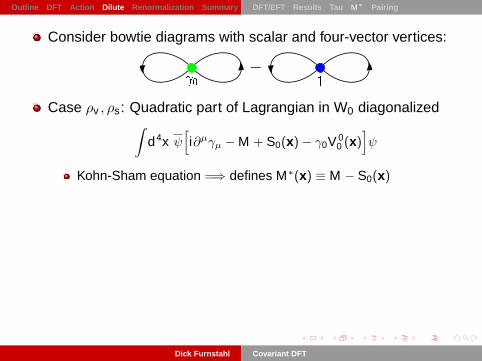
Outline DFT Action Dilute Renormalization Summary DFT/EFT Results Tau M∗ Pairing
Consider bowtie diagrams with scalar and four-vector vertices:
Case ρv , ρs: Quadratic part of Lagrangian in W0 diagonalized∫d4x ψ
[i∂µγµ −M + S0(x)− γ0V 0
0 (x)]ψ
Kohn-Sham equation =⇒ defines M∗(x) ≡ M − S0(x)
Case ρv : Quadratic part of Lagrangian in W0 diagonalized∫d4x ψ
[i∂µγµ −M − γ0V 0
0 (x)]ψ
Scalar diagram evaluated in LDA
How do observables compare?Binding energies, densitiesWhat about the single-particle spectra?
Dick Furnstahl Covariant DFT

Outline DFT Action Dilute Renormalization Summary DFT/EFT Results Tau M∗ Pairing
Kohn-Sham LDA ρv vs. ρv , ρs
0 1 2 3 4 5r (fm)
0
0.05
0.1
0.15
0.2
0.25ρ P (f
m-3
)ρv/ρs, A = 16ρv, A = 16ρv/ρs, A = 40ρv, A=40
Dick Furnstahl Covariant DFT
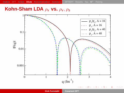
Outline DFT Action Dilute Renormalization Summary DFT/EFT Results Tau M∗ Pairing
Kohn-Sham LDA ρv vs. ρv , ρs
0 1 2 3 4
q (fm-1)
0.001
0.01
0.1
1|F
(q)|
ρv/ρs, A = 16ρv, A = 16ρv/ρs, A = 40ρv, A = 40
Dick Furnstahl Covariant DFT

Outline DFT Action Dilute Renormalization Summary DFT/EFT Results Tau M∗ Pairing
Kohn-Sham LDA ρv vs. ρv , ρs: Differences
A = 16 BE/A√〈r2〉
ρv 27.5 1.97ρv , ρs 27.1 1.99
A = 40 BE/A√〈r2〉
ρv 29.4 2.57ρv , ρs 27.8 2.56
0 1 2 3 4 5r (fm)
-0.02
-0.01
0
0.01
0.02
∆ρP (f
m-3
)
Dick Furnstahl Covariant DFT

Outline DFT Action Dilute Renormalization Summary DFT/EFT Results Tau M∗ Pairing
Energy Spectra ρv , ρs vs. ρv
-60
-50
-40
-30
-20
bind
ing
ener
gy (M
eV)
1s1/2
1p3/2
1p1/2
A = 16
ρv,ρsρv -70
-60
-50
-40
-30
-20
bind
ing
ener
gy (M
eV)
1s1/2
1p3/2
1p1/2
A = 40
ρv,ρsρv
1d5/2
1d3/2
2s1/2
Dick Furnstahl Covariant DFT

Outline DFT Action Dilute Renormalization Summary DFT/EFT Results Tau M∗ Pairing
How is the Full G Related to Gks?
+ + + + · · · =⇒ = +x′
x=⇒ Σ∗(x,x′;ω)
Add a non-local source ξ(x ′, x) coupled to ψ†(x ′)ψ(x):
Z [J, ξ] = eiW [J,ξ] =
∫DψDψ† ei
∫d4x [L+ J(x)ψ†(x)ψ(x) +
∫d4x′ ξ(x′,x)ψ†(x′)ψ(x)]
With Γ[ρ, ξ] = Γ0[ρ, ξ] + Γint[ρ, ξ],
G(x , x ′) =δWδξ
∣∣∣∣J
=δΓ
δξ
∣∣∣∣ρ
= Gks(x , x ′) + Gks
[ δΓint
δGks− δΓint
δρ
]Gks
Dick Furnstahl Covariant DFT

Outline DFT Action Dilute Renormalization Summary DFT/EFT Results Tau M∗ Pairing
How Do G and Gks Yield the Same Density?
Claim: ρks(x) = −iνG0KS(x , x+) equals ρ(x) = −iνG(x , x+)
Start with
Simple diagrammatic demonstration:
Densities agree by construction!
But other observables may differ; spectral functions?
Dick Furnstahl Covariant DFT

Outline DFT Action Dilute Renormalization Summary DFT/EFT Results Tau M∗ Pairing
Pairing in DFT/EFT from Effective Action
Natural framework for spontaneous symmetry breakinge.g., test for zero-field magnetization M in a spin systemintroduce an external field H to break rotational symmetryLegendre transform Helmholtz free energy F (H):
invert M = −∂F (H)/∂H =⇒ G[M] = F [H(M)] + MH(M)
since H = ∂G/∂M, minimize G to find ground state
Dick Furnstahl Covariant DFT
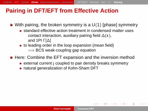
Outline DFT Action Dilute Renormalization Summary DFT/EFT Results Tau M∗ Pairing
Pairing in DFT/EFT from Effective Action
With pairing, the broken symmetry is a U(1) [phase] symmetrystandard effective action treatment in condensed matter uses
contact interaction, auxiliary pairing field ∆(x),and 1PI Γ[∆]
to leading order in the loop expansion (mean field)=⇒ BCS weak-coupling gap equation
Here: Combine the EFT expansion and the inversion methodexternal current j coupled to pair density breaks symmetrynatural generalization of Kohn-Sham DFT
Dick Furnstahl Covariant DFT

Outline DFT Action Dilute Renormalization Summary DFT/EFT Results Tau M∗ Pairing
Generalizing Effective Action to Include Pairing
Generating functional with sources J, j coupled to densities:
Z [J, j] = e−W [J,j] =
∫D(ψ†ψ) e−
∫d4x [L+ J(x)ψ†
αψα + j(x)(ψ†↑ψ
†↓+ψ↓ψ↑)]
Densities found by functional derivatives wrt J, j :
ρ(x) ≡ 〈ψ†(x)ψ(x)〉J,j =δW [J, j]δJ(x)
∣∣∣∣j
φ(x) ≡ 〈ψ†↑(x)ψ†↓(x) + ψ↓(x)ψ↑(x)〉J,j =δW [J, j]δj(x)
∣∣∣∣J
Effective action Γ[ρ, φ] by functional Legendre transformation:
Γ[ρ, φ] = W [J, j]−∫
d4x J(x)ρ(x)−∫
d4x j(x)φ(x)
Dick Furnstahl Covariant DFT

Outline DFT Action Dilute Renormalization Summary DFT/EFT Results Tau M∗ Pairing
Γ[ρ, φ] ∝ ground-state (free) energy functional E [ρ, φ]
at finite temperature, the proportionality constant is β
The sources are given by functional derivatives wrt ρ and φ
δE [ρ, φ]
δρ(x)= J(x) and
δE [ρ, φ]
δφ(x)= j(x)
but the sources are zero in the ground state=⇒ determine ground-state ρ(x) and φ(x) by stationarity:
δE [ρ, φ]
δρ(x)
∣∣∣∣ρ=ρgs,φ=φgs
=δE [ρ, φ]
δφ(x)
∣∣∣∣ρ=ρgs,φ=φgs
= 0
This is Hohenberg-Kohn DFT extended to pairing!
We need a method to carry out the inversionFor Kohn-Sham DFT, apply inversion methodsWe need to renormalize!
Dick Furnstahl Covariant DFT

Outline DFT Action Dilute Renormalization Summary DFT/EFT Results Tau M∗ Pairing
Kohn-Sham Inversion Method Revisited
Order-by-order matching in EFT expansion parameter λ
J[ρ, φ, λ] = J0[ρ, φ] + J1[ρ, φ] + J2[ρ, φ] + · · ·j[ρ, φ, λ] = j0[ρ, φ] + j1[ρ, φ] + j2[ρ, φ] + · · ·
W [J, j , λ] = W0[J, j] + W1[J, j] + W2[J, j] + · · ·Γ[ρ, φ, λ] = Γ0[ρ, φ] + Γ1[ρ, φ] + Γ2[ρ, φ] + · · ·
0th order is Kohn-Sham system with potentials J0(x) and j0(x)=⇒ yields the exact densities ρ(x) and φ(x)
introduce single-particle orbitals and solve(h0(x)− µ0 j0(x)
j0(x) −h0(x) + µ0
)(ui(x)vi(x)
)= Ei
(ui(x)vi(x)
)
where h0(x) ≡ −∇2
2M+ v(x)− J0(x)
with conventional orthonormality relations for ui , vi
Dick Furnstahl Covariant DFT

Outline DFT Action Dilute Renormalization Summary DFT/EFT Results Tau M∗ Pairing
Diagrammatic Expansion of Wi
Same diagrams, but with Nambu-Gor’kov Green’s functions
Γint = + + + + · · ·
iG =
(〈Tψ↑(x)ψ†↑(x
′)〉0 〈Tψ↑(x)ψ↓(x ′)〉0〈Tψ†↓(x)ψ†↑(x
′)〉0 〈Tψ†↓(x)ψ↓(x ′)〉0
)≡
(iG0
ks iF 0ks
iF 0ks† −iG0
ks
)In frequency space, the Green’s functions are
iG0ks(x, x
′;ω) =∑
i
[ui(x) u∗i (x′)ω − Ei + iη
+vi(x′) v∗i (x)
ω + Ei − iη
]
iF 0ks(x, x
′;ω) = −∑
i
[ui(x) v∗i (x′)ω − Ei + iη
−ui(x′) v∗i (x)
ω + Ei − iη
]
Dick Furnstahl Covariant DFT

Outline DFT Action Dilute Renormalization Summary DFT/EFT Results Tau M∗ Pairing
Kohn-Sham Self-Consistency Procedure
Same iteration procedure as in Skyrme or RMF with pairing
In terms of the orbitals, the fermion density is
ρ(x) = 2∑
i
|vi(x)|2
and the pair density is (warning: divergent!)
φ(x) =∑
i
[u∗i (x)vi(x) + ui(x)v∗i (x)]
The chemical potential µ0 is fixed by∫ρ(x) = A
Diagrams for Γ[ρ, φ] = −E [ρ, φ] (with LDA+) yields KS potentials
J0(x)∣∣∣ρ=ρgs
=δΓint[ρ, φ]
δρ(x)
∣∣∣∣∣ρ=ρgs
and j0(x)∣∣∣φ=φgs
=δΓint[ρ, φ]
δφ(x)
∣∣∣∣∣φ=φgs
Dick Furnstahl Covariant DFT

Outline DFT Action Dilute Renormalization Summary DFT/EFT Results Tau M∗ Pairing
Divergences: Uniform SystemGenerating functional with constant sources µ and j :
e−W =
∫D(ψ†ψ) e−
∫d4x [ψ†
α( ∂∂τ −
∇ 22M −µ)ψα +
C02 ψ
†↑ψ
†↓ψ↓ψ↑+ j(ψ↑ψ↓+ψ†
↓ψ†↑)]
+ 12 ζ j2
cf. adding integration over auxiliary field∫
D(∆∗,∆) e−1
|C0|∫|∆|2
=⇒ shift variables to eliminate ψ†↑ψ†↓ψ↓ψ↑ for ∆∗ψ↑ψ↓
New divergences because of j =⇒ e.g., expand to O(j2)
Same linear divergence as in 2-to-2 scattering
Strategy: Add counterterm 12ζ j2 to L
additive to W (cf. |∆|2) =⇒ no effect on scatteringEnergy interpretation? Finite part?
Dick Furnstahl Covariant DFT

Outline DFT Action Dilute Renormalization Summary DFT/EFT Results Tau M∗ Pairing
Divergences: Uniform SystemGenerating functional with constant sources µ and j :
e−W =
∫D(ψ†ψ) e−
∫d4x [ψ†
α( ∂∂τ −
∇ 22M −µ)ψα +
C02 ψ
†↑ψ
†↓ψ↓ψ↑+ j(ψ↑ψ↓+ψ†
↓ψ†↑)] + 1
2 ζ j2
cf. adding integration over auxiliary field∫
D(∆∗,∆) e−1
|C0|∫|∆|2
=⇒ shift variables to eliminate ψ†↑ψ†↓ψ↓ψ↑ for ∆∗ψ↑ψ↓
New divergences because of j =⇒ e.g., expand to O(j2)
Same linear divergence as in 2-to-2 scattering
Strategy: Add counterterm 12ζ j2 to L
additive to W (cf. |∆|2) =⇒ no effect on scatteringEnergy interpretation? Finite part?
Dick Furnstahl Covariant DFT

Outline DFT Action Dilute Renormalization Summary DFT/EFT Results Tau M∗ Pairing
Kohn-Sham Non-interacting System
Canonical Bogoliubov transformation solves exactly
W0[µ0, j0] =
∫d3k
(2π)3 (ξk − Ek ) +12ζ(0)j20
where ξk ≡ ε0k − µ0 and Ek ≡√ξ2
k + j20
Kohn-Sham potential j0 plays the role of a constant gap
µ0
0
1
εk
vk2 uk
2
j0
ρ = 2∑
k
v2k =
∫d3k
(2π)3
(1− ξk
Ek
)φ = 2
∑k
uk vk = −∫
d3k(2π)3
j0Ek
+ ζ(0)j0
Dick Furnstahl Covariant DFT

Outline DFT Action Dilute Renormalization Summary DFT/EFT Results Tau M∗ Pairing
Renormalizing the “Gap” Equation
Leading-order (LO) calculation requires Γ1[ρ, φ] =⇒ j1 = δΓ1/δφ ∼ C0Tr F + CTC
Choose LO counterterms (“CTC”) so that Γ1 is a function of ρand the renormalized φ only
“Gap” equation from j = j0 + j1 = 0 =⇒ linear divergence
j0 = −j1 = −12|C0|φ
uniform=
12|C0| j0
∫ d3k(2π)3
1√(ε0
k − µ0)2 + j20
− ζ(0)
Conventional approach: Subtract equation for as to eliminate C0
M4πas
+1|C0|
=12
∫d3k
(2π)3
1ε0
k
=⇒ M4πas
= −12
∫d3k
(2π)3
[1
Ek− 1ε0
k
]
Dick Furnstahl Covariant DFT
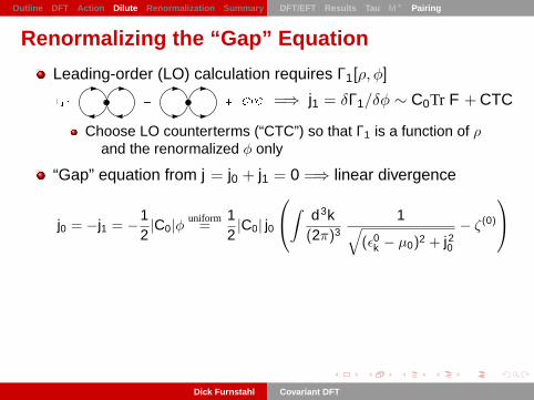
Outline DFT Action Dilute Renormalization Summary DFT/EFT Results Tau M∗ Pairing
Observables With Kohn-Sham Pairing
To find the energy density, evaluate Γ at the stationary point:
EV
= (Γ0 + Γ1)|j0=− 12 |C0|φ =
∫d3k
(2π)3
[ξk −Ek +
12
j20Ek
]+[µ0 −
14|C0|ρ
]ρ
with
ρ =
∫d3k
(2π)3
(1− ξk
Ek
)and φ = −
∫d3k
(2π)3
j0Ek
+ ζ(0)j0
Explicitly finite and dependence on ζ(0) cancels out
Recover normal state from j0 → 0:
EV→ 3
5µ0ρ−
14|C0|ρ2 and ρ→ 1
3π2 k3F and µ0 →
k2F
2M
Dick Furnstahl Covariant DFT

Outline DFT Action Dilute Renormalization Summary DFT/EFT Results Tau M∗ Pairing
Dimensional Regularization (DR)
DR/PDS =⇒ explicit Λ to “check” for cutoff dependencecf. Papenbrock & Bertsch DR/MS calculation =⇒ Λ = 0
C0(Λ) =4πas
M1
1− asΛ=
4πas
M+
4πa2s
MΛ +O(Λ2) = C(1)
0 + C(2)0 + · · ·
Basic free-space integral =⇒ beachball renormalization in Γ2:(Λ
2
)3−D ∫ dDu(2π)D
1t2 − u2 + iε
PDS−→ − 14π
(Λ + it)
=⇒ independent of Λ
Dick Furnstahl Covariant DFT

Outline DFT Action Dilute Renormalization Summary DFT/EFT Results Tau M∗ Pairing
Dimensional Regularization and Pairing
The basic DR/PDS integral in D dimensions, with x ≡ j0/µ0, is
I(β) ≡(Λ
2
)3−D∫
dDk(2π)D
(ε0k )β
Ek=
MΛ
2πµβ0
(1− δβ,2
x2
2
)+ (−)β+1 M3/2
√2π
[µ20(1 + x2)](β+1/2)/2 P0
β+1/2
( −1√1 + x2
)
Check the density equation =⇒ Λ dependence cancels:
ρ =
∫d3k
(2π)3
(1−
ε0k − µ0
Ek
)= 0− I(1) + µ0 I(0)
The gap equation implies ζ(0) is naturally taken from 1/C0(Λ):
1|C0(Λ)|
=12
I(0) or1|C0|
=12
(I(0)− ζ(0)
)
Dick Furnstahl Covariant DFT

Outline DFT Action Dilute Renormalization Summary DFT/EFT Results Tau M∗ Pairing
Dimensional Regularization and Pairing
The basic DR/PDS integral in D dimensions, with x ≡ j0/µ0, is
I(β) ≡(Λ
2
)3−D∫
dDk(2π)D
(ε0k )β
Ek=
MΛ
2πµβ0
(1− δβ,2
x2
2
)+ (−)β+1 M3/2
√2π
[µ20(1 + x2)](β+1/2)/2 P0
β+1/2
( −1√1 + x2
)Check the density equation =⇒ Λ dependence cancels:
ρ =
∫d3k
(2π)3
(1−
ε0k − µ0
Ek
)= 0− I(1) + µ0 I(0)
The gap equation implies ζ(0) is naturally taken from 1/C0(Λ):
1|C0(Λ)|
=12
I(0) or1|C0|
=12
(I(0)− ζ(0)
)Dick Furnstahl Covariant DFT

Outline DFT Action Dilute Renormalization Summary DFT/EFT Results Tau M∗ Pairing
Anomalous Density in Finite Systems
How do we renormalize the pair density in a finite system?
φ(x) =∑
i
[u∗i (x)vi(x) + ui(x)v∗i (x)] −→∞
cf. scalar density ρs =∑
i ψ(x)ψ(x) for solitons or relativistic nuclei
In the uniform limit, φ can be defined with a subtraction
φ =
∫ kc d3k(2π)3 j0
1√(ε0
k − µ0)2 + j20
− 1ε0
k
kc→∞−→ finite
Apply this in a local density approximation (Thomas-Fermi)
φ(x) = 2Ec∑i
ui(x)vi(x)− j0(x)M kc(x)
2π2 with Ec =k2
c (x)
2M+ vKS(x)− µ
Dick Furnstahl Covariant DFT
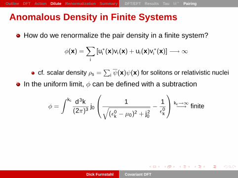
Outline DFT Action Dilute Renormalization Summary DFT/EFT Results Tau M∗ Pairing
Bulgac Renormalization [Bulgac/Yu PRL 88 (2002) 042504]
Convergence is very slow as the energy cutoff is increased=⇒ Bulgac/Yu: make a different subtraction
φ =
∫ kc d3k(2π)3 j0
1√(ε0
k − µ0)2 + j20
− Pε0
k − µ0
kc→∞−→ finite
Compare convergence in uniform system and in nuclei with LDA
0.01 0.1 1 10Energy Cutoff
10-6
10-5
10-4
10-3
10-2
10-1
100
Frac
tion
Mis
sing
subtraction 1subtraction 2
µ0 = 1j0 = 0.1
0 2 4 6 8 10 120
0.5
1
1.5
2
2.5
r [fm]
∆(r
) [M
eV]
Dick Furnstahl Covariant DFT

Outline DFT Action Dilute Renormalization Summary DFT/EFT Results Tau M∗ Pairing
Even Better! [Bulgac, PRC 65 (2002) 051305]
Convergence is rapid above Fermi surface but not below=⇒ scale set by Fermi energy rather than gap
Solution: Energy cutoff around µ
0 5 10 15 20 25−50
−40
−30
−20
−10
0
r [fm]
U(r
) [M
eV]
µ + Ec
µ
µ − Ec
r1
r2
I II III
5 10 15 20 25 30 35 40 45 500
1
2
3
4
∆ [M
eV]
5 10 15 20 25 30 35 40 45 50−600
−500
−400
−300
−200
−100
Ec [MeV]
g eff [M
eV fm
3 ]
Dick Furnstahl Covariant DFT
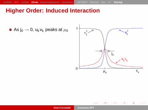
Outline DFT Action Dilute Renormalization Summary DFT/EFT Results Tau M∗ Pairing
Higher Order: Induced Interaction
As j0 → 0, ukvk peaks at µ0
Leading order T = 0:∆LO/µ0 = 8
e2 e−1/N(0)|C0|
= 8e2 e−π/2kF|as|
NLO modifies exponent=⇒ changes prefactor
∆NLO ≈ ∆LO/(4e)1/3
µ0
0
1
εk
vk2 uk
2
j0ukvk
Dick Furnstahl Covariant DFT

Outline DFT Action Dilute Renormalization Summary DFT/EFT Results Tau M∗ Pairing
Higher Order: Induced Interaction
As j0 → 0, ukvk peaks at µ0
Leading order T = 0:∆LO/µ0 = 8
e2 e−1/N(0)|C0|
= 8e2 e−π/2kF|as|
NLO modifies exponent=⇒ changes prefactor
∆NLO ≈ ∆LO/(4e)1/3
µ0
0
1
εk
vk2 uk
2
j0
ukvk
Dick Furnstahl Covariant DFT
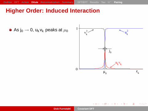
Outline DFT Action Dilute Renormalization Summary DFT/EFT Results Tau M∗ Pairing
Higher Order: Induced Interaction
As j0 → 0, ukvk peaks at µ0
Leading order T = 0:∆LO/µ0 = 8
e2 e−1/N(0)|C0|
= 8e2 e−π/2kF|as|
NLO modifies exponent=⇒ changes prefactor
∆NLO ≈ ∆LO/(4e)1/3
µ0
0
1
εk
vk2 uk
2
j0
ukvk
Dick Furnstahl Covariant DFT
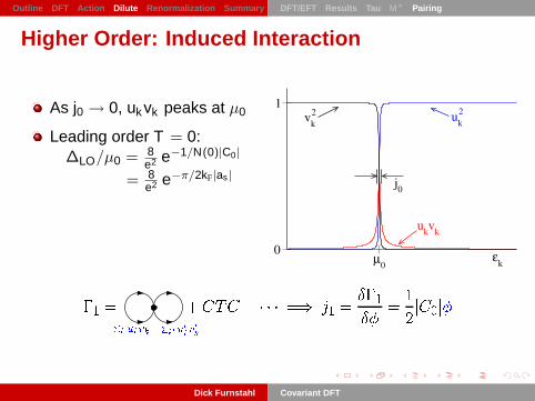
Outline DFT Action Dilute Renormalization Summary DFT/EFT Results Tau M∗ Pairing
Higher Order: Induced Interaction
As j0 → 0, ukvk peaks at µ0
Leading order T = 0:∆LO/µ0 = 8
e2 e−1/N(0)|C0|
= 8e2 e−π/2kF|as|
NLO modifies exponent=⇒ changes prefactor
∆NLO ≈ ∆LO/(4e)1/3
µ0
0
1
εk
vk2 uk
2
j0
ukvk
Dick Furnstahl Covariant DFT

Outline DFT Action Dilute Renormalization Summary DFT/EFT Results Tau M∗ Pairing
Higher Order: Induced Interaction
As j0 → 0, ukvk peaks at µ0
Leading order T = 0:∆LO/µ0 = 8
e2 e−1/N(0)|C0|
= 8e2 e−π/2kF|as|
NLO modifies exponent=⇒ changes prefactor
∆NLO ≈ ∆LO/(4e)1/3 µ0
0
1
εk
vk2 uk
2
j0
ukvk
! " $#% '&)(+*(-, (.*/0(-,2143 56 7
Dick Furnstahl Covariant DFT

Outline DFT Action Dilute Renormalization Summary DFT/EFT Results Tau M∗ Pairing
Covariant Pairing
Point-coupling version of Capelle and Gross [PRB 59 (1999) 7140]Dirac-Bogoliubov-de Gennes equations
Couple to time-reversed pairs with definite Lorentz nature
Same basic DFT treatment with scalar source coupled to
ψTη0ψ with η0 ≡ γ1γ3
and zero-component of four-vector source coupled to
ψTη0vψ with η0
v ≡ γ0γ1γ3
Dick Furnstahl Covariant DFT
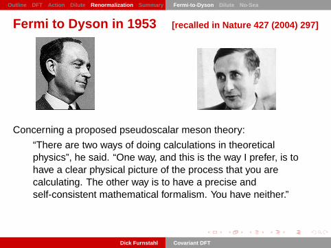
Outline DFT Action Dilute Renormalization Summary Fermi-to-Dyson Dilute No-Sea
Fermi to Dyson in 1953 [recalled in Nature 427 (2004) 297]
Concerning a proposed pseudoscalar meson theory:
“There are two ways of doing calculations in theoreticalphysics”, he said. “One way, and this is the way I prefer, is tohave a clear physical picture of the process that you arecalculating. The other way is to have a precise andself-consistent mathematical formalism. You have neither.”
Dick Furnstahl Covariant DFT

Outline DFT Action Dilute Renormalization Summary Fermi-to-Dyson Dilute No-Sea
Fermi to Dyson in 1953 [recalled in Nature 427 (2004) 297]
I was slightly stunned, but ventured to ask him why he didnot consider the pseudoscalar meson theory to be aself-consistent mathematical formalism. He replied,“Quantum electrodynamics is a good theory because theforces are weak, and when the formalism is ambiguous wehave a clear physical picture to guide us. With thepseudoscalar meson theory there is no physical picture, andthe forces are so strong that nothing converges. To reachyour calculated results, you had to introduce arbitrary cut-offprocedures that are not based either on solid physics or onsolid mathematics.”
Dick Furnstahl Covariant DFT

Outline DFT Action Dilute Renormalization Summary Fermi-to-Dyson Dilute No-Sea
UV Divergences in Nonrelativisticand Relativistic Effective Actions
Sensitivity to short-distance physics signalled by divergencesbut finiteness (e.g., with cutoff) doesn’t mean not sensitive!=⇒ must absorb sensitivity via renormalization
Sources of UV divergences
nonrelativistic covariantscattering scattering
pairing pairinganti-nucleons
Dick Furnstahl Covariant DFT

Outline DFT Action Dilute Renormalization Summary Fermi-to-Dyson Dilute No-Sea
Power Counting Lost / Power Counting Regained
Gasser, Sainio, and Svarc =⇒ ChPT for πN with relativistic N’sloop and momentum expansions don’t agree
=⇒ systematic power counting lostheavy-baryon EFT restores power counting by 1/M expansion
Hua-Bin Tang (1996) [and with Paul Ellis]:
q > Λ
VB
VB
=⇒ C0 and
µ +M−Mωx x
negative−energy states
x x x xx x x
x x x
holes
positive−energy states
x x x x
Dick Furnstahl Covariant DFT

Outline DFT Action Dilute Renormalization Summary Fermi-to-Dyson Dilute No-Sea
Power Counting Lost / Power Counting Regained
Gasser, Sainio, and Svarc =⇒ ChPT for πN with relativistic N’sloop and momentum expansions don’t agree
=⇒ systematic power counting lostheavy-baryon EFT restores power counting by 1/M expansion
Hua-Bin Tang (1996) [and with Paul Ellis]:
“. . . EFT’s permit useful low-energy expansions only if we ab-sorb all of the hard-momentum effects into the parameters ofthe Lagrangian.”
q > Λ
VB
VB
=⇒ C0 and
µ +M−Mωx x
negative−energy states
x x x xx x x
x x x
holes
positive−energy states
x x x x
Dick Furnstahl Covariant DFT

Outline DFT Action Dilute Renormalization Summary Fermi-to-Dyson Dilute No-Sea
Power Counting Lost / Power Counting Regained
Gasser, Sainio, and Svarc =⇒ ChPT for πN with relativistic N’sloop and momentum expansions don’t agree
=⇒ systematic power counting lostheavy-baryon EFT restores power counting by 1/M expansion
Hua-Bin Tang (1996) [and with Paul Ellis]:
“When we include the nucleons relativistically, the anti-nucleon contributions are also hard-momentum effects.”
q > Λ
VB
VB
=⇒ C0 and
µ +M−Mωx x
negative−energy states
x x x xx x x
x x x
holes
positive−energy states
x x x x
Dick Furnstahl Covariant DFT
Outline DFT Action Dilute Renormalization Summary Fermi-to-Dyson Dilute No-Sea
Moving Dirac Sea Physics into Coefficients
Absorb the “hard” part of a diagram into parameters,=⇒ the remaining “soft” part satisfies chiral power counting
original πN prescription by H.B. Tang (expand,integrate term-by-term, and resum propagators)
systematized for πN by Becher and Leutwyler:“infrared regularization” or IR
not unique; e.g., Fuchs et al. additional finite subtractions in DR
Extension of IR to multiple heavy particles [Lehmann and Prezeau]convenient reformulation by Schindler, Gegelia, Schererparticle-particle loop reduces to nonrelativistic DR/MS resultparticle-hole loops in free space vanish!
Dick Furnstahl Covariant DFT

Outline DFT Action Dilute Renormalization Summary Fermi-to-Dyson Dilute No-Sea
Consequences for Free-Space Natural Fermions
Leading order (LO) has scalar, vector, etc. vertices
Dick Furnstahl Covariant DFT

Outline DFT Action Dilute Renormalization Summary Fermi-to-Dyson Dilute No-Sea
Consequences for Free-Space Natural Fermions
At NLO, only particle-particle loop survives IR
Only forward-going nucleons contribute=⇒ same result as nonrel. DR/MS for small k
Dick Furnstahl Covariant DFT

Outline DFT Action Dilute Renormalization Summary Fermi-to-Dyson Dilute No-Sea
Consequences for Free-Space Natural Fermions
At NNLO, only particle-particle loop diagram survives IR
All other diagrams are zero in IR
Dick Furnstahl Covariant DFT
Outline DFT Action Dilute Renormalization Summary Fermi-to-Dyson Dilute No-Sea
Effective Action and Subtraction Prescription
Use effective action formalism to carry out EFT at finite densityKohn-Sham DFT using inversion methodW0[S0,V
µ0 ] with Kohn-Sham potentials S0,V
µ0
Zeroth order =⇒ non-interacting system=⇒ Tr ln(i 6∂ + µγ0 −M∗ − gv6V0) ≡ Tr ln G−1
KS (µ)Divergences as with pairing =⇒ counterterms in IR
Subtraction prescription: Define CT’s to cancel Tr ln at µ = 0Derivative expansion: −i Tr ln(i 6∂ −M∗ − gv6V0) =∫
d4x [Ueff(S0) + 12 Z1s(S0)∂µS0 ∂
µS0 + · · · ] ≡ − CT’s
=⇒ local polynomial in the fields: CT’s ⇐⇒ iTr ln G−1KS (0)
Shifts “hard” Dirac sea physics into coefficientsuse same coefficients for any Kohn-Sham fields S0(x),Vµ
0 (x)use the ground state problem to subtract at µ = 0
=⇒ fixed consequences for treating linear response (RPA)
Dick Furnstahl Covariant DFT

Outline DFT Action Dilute Renormalization Summary Fermi-to-Dyson Dilute No-Sea
“No-Sea Approximation” for the Ground State
Self-consistent equations for S0,Vµ0 from extremizing Γ[jµ, ρs]
these determine static S0(x) and V0(x) for ground state
Γ with gs densities is proportional to the (free) energyG−1
KS (µ) is diagonal in the single-particle basis ψα(x)eiωx0
replace CT’s in Γ with +i Tr ln G−1KS (0) (using S0(x),V0(x))
so W0 = −i Tr ln G−1KS (µ) + i Tr ln G−1
KS (0)
=⇒εα<µ∑α
(µ− εα)−εα<0∑α
(−εα)− [vac. sub.] =
0<εα<µ∑α
(µ− εα)
Similarly, for ρs(x) ∝ δW0/δS0(x) =⇒ Tr GKS(µ)− Tr GKS(0)
εα<µ∑
α
h−x −
εα<0∑
α
−x =
0<εα<µ∑
α
h
x
=⇒ we recover the “no-sea approximation” for the ground state
Dick Furnstahl Covariant DFT

Outline DFT Action Dilute Renormalization Summary Fermi-to-Dyson Dilute No-Sea
Consider Γ[jµ, ρs] with time-dependent fluctuations=⇒ S0(x) = S0(x) + S(x) V µ
0 (x) = V0(x) δµ0 + V µ(x)Γ is the generator of 1PI Green’s functions
=⇒ linear response from 2nd order terms in S, Vµ
CT’s =⇒ +i Tr ln G−1(0) still holds with S(x),Vµ(x)!
Expand −i Tr ln G−1(µ) + i Tr ln G−1(0) + . . . in S, V µ
ln(G−1KS + S) = ln(G−1
KS )[. . .− 1
2 GKS · S ·GKS · S + . . .]
so the contributions to RPA rings from the Tr ln’s are:
−i Tr ln G−1(µ) =⇒ p h + p − −i Tr ln G−1(0) =⇒ + −
Combining (only well defined together!) . . .
p h + p − − + − = p h − h −
=⇒ Subtraction prescription for RPA: include ph and h− pairs
Dick Furnstahl Covariant DFT

Outline DFT Action Dilute Renormalization Summary Fermi-to-Dyson Dilute No-Sea
Covariant EFT and Negative-Energy States
EFT: Absorb hard-momentum Dirac-sea physics into parameters
Good RMF/RPA “no-sea” phenomenology explained by EFTQCD vacuum effects automatically encoded in fit parameters!in principle we need all counterterms;
in practice under-determinedrelies on naturalness for usual truncation
Dick Furnstahl Covariant DFT

Outline DFT Action Dilute Renormalization Summary Future Answers
On-Going and Future Challenges
Covariant diluteFermi system
Long-range effects
Gradient expansions
Auxiliary fieldKohn-Sham Theory
Restoring brokensymmetries
Dick Furnstahl Covariant DFT

Outline DFT Action Dilute Renormalization Summary Future Answers
On-Going and Future Challenges
Covariant diluteFermi system
Long-range effects
Gradient expansions
Auxiliary fieldKohn-Sham Theory
Restoring brokensymmetries
Controlled laboratory for finite systemCompare to heavy baryon EFTFocus on spin-orbitThree-body forces?
Covariant pairingInduced interaction
Time-dependent Kohn-Sham theoryHigher order in effective action
formalismKohn-Sham part =⇒ RPAPoint-coupling version?
Dick Furnstahl Covariant DFT

Outline DFT Action Dilute Renormalization Summary Future Answers
On-Going and Future Challenges
Covariant diluteFermi system
Long-range effects
Gradient expansions
Auxiliary fieldKohn-Sham Theory
Restoring brokensymmetries
Long-range forces (e.g., pion exchange)
Non-localities from near-on-shellparticle-hole excitations
+ + + + · · ·
Dick Furnstahl Covariant DFT

Outline DFT Action Dilute Renormalization Summary Future Answers
On-Going and Future Challenges
Covariant diluteFermi system
Long-range effects
Gradient expansions
Auxiliary fieldKohn-Sham Theory
Restoring brokensymmetries
Semiclassical expansions usedin Coulomb DFT
Gradient expansion techniques for(one-loop) effective actions
Dick Furnstahl Covariant DFT

Outline DFT Action Dilute Renormalization Summary Future Answers
On-Going and Future Challenges
Covariant diluteFermi system
Long-range effects
Gradient expansions
Auxiliary fieldKohn-Sham Theory
Restoring brokensymmetries
Auxiliary fields correspond tonon-dynamical meson fields
Apply saddlepoint evaluationrequiring density to be unchanged
Faussier and Valiev/Fernando formalism,but no higher-order calculations yet
How to separate ph and pp for pairing?
Revisit large N expansion?
Dick Furnstahl Covariant DFT

Outline DFT Action Dilute Renormalization Summary Future Answers
On-Going and Future Challenges
Covariant diluteFermi system
Long-range effects
Gradient expansions
Auxiliary fieldKohn-Sham Theory
Restoring brokensymmetries
Translational and rotational invariance,particle number
Not addressed in Coulomb DFT
Energy functional for the intrinsic density?[Engel, Furnstahl, Schwenk]
Dick Furnstahl Covariant DFT

Outline DFT Action Dilute Renormalization Summary Future Answers
Should we connect to the free NN interaction?In Coulomb DFT, Hartree-Fock gives dominate contribution
=⇒ correlations are small corrections =⇒ gradient expansion
cf. conventional NN interactions =⇒ correlations Hartree-Fock
But if we run a cutoff toward the Fermi surface . . .
F: |P/2 ± k| < kF
Λ: |P/2 ± k| > kF
P/2
k
Λ
kF
|k| < Λand
Match at finite density =⇒ perturbative?
Dick Furnstahl Covariant DFT

Outline DFT Action Dilute Renormalization Summary Future Answers
Summary Comments on Vacuum Physics
Unlike QED DFT, “no sea” for nuclear structure is a misnomerinclude “vacuum physics” in coefficients through renormalization
Renormalization versus RenormalizabilityRenormalization is required to account for short-distance
behavior but can be implicitRenormalizability at the hadronic level corresponds to making
a model for the short-distance behaviornot a good model phenomenologically
Fixing short-distance behavior is not the same thing asthrowing away negative-energy states
For a long time, we looked for unique “relativistic effects”;these were largely misguided efforts
Dick Furnstahl Covariant DFT


