CSCI-2950-uSwitching and Routing
Overview
Most slides from CS-168
Rodrigo Fonseca
Switched Ethernet
• Most common link layer today• Most popular bandwidths: 1Gbps,
10Gbps, 40Gbps growing• All switched, in practice– No CSMA-CD

Ethernet Addressing• Globally unique, 48-bit unicast
address per adapter– Example: 00:1c:43:00:3d:09 (Samsung
adapter)– 24 msb: organization– http://standards.ieee.org/develop/regauth/
oui/oui.txt
• Broadcast address: all 1s• Multicast address: first bit 1• Adapter can work in promiscuous
mode

Scaling
• Direct-link networks don’t scale
• Solution: use switches to connect network segments

Bridges and Extended LANs• LANs have limitations– E.g. Ethernet < 1024 hosts, < 2500m
• Connect two or more LANs with a bridge– Operates on Ethernet addresses– Forwards packets from one LAN to the
other(s)
• Ethernet switch is just a multi-way bridge

Learning Bridges
• Idea: don’t forward a packet where it isn’t needed– If you know recipient is not on that port
• Learn hosts’ locations based on source addresses– Build a table as you receive packets– Table is a cache: if full, evict old entries. Why is this fine?
• Table says when not to forward a packet– Doesn’t need to be complete for correctness

Bridges
• Unicast: forward with filtering• Broadcast: always forward• Multicast: always forward or learn
groups• Difference between bridges and
repeaters?– Bridges: same broadcast domain; copy
frames– Repeaters: same broadcast and collision
domain; copy signals

Dealing with Loops• Problem: people may create loops
in LAN!– Accidentally, or to provide redundancy– Don’t want to forward packets indefinitely
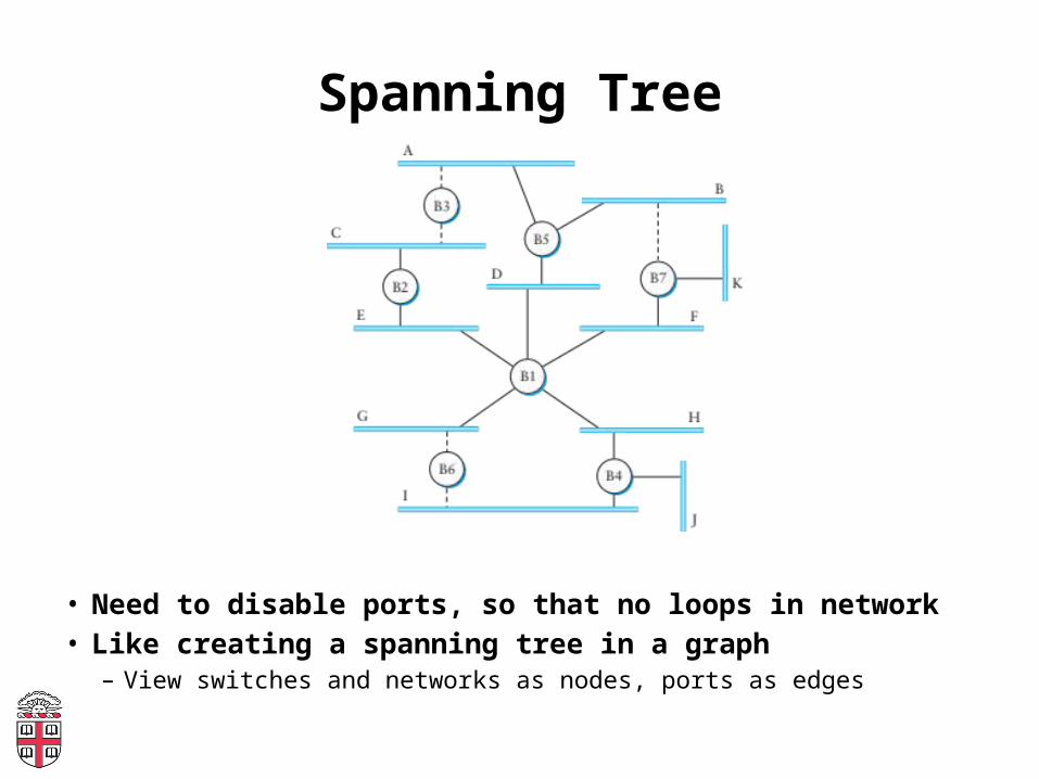
Spanning Tree
• Need to disable ports, so that no loops in network• Like creating a spanning tree in a graph
– View switches and networks as nodes, ports as edges

Distributed Spanning Tree Algorithm
• Every bridge has a unique ID (Ethernet address)
• Goal:– Bridge with the smallest ID is the root– Each segment has one designated bridge,
responsible for forwarding its packets towards the root• Bridge closest to root is designated bridge• If there is a tie, bridge with lowest ID wins

Spanning Tree Protocol
• Spanning Tree messages contain:– ID of bridge sending the message– ID sender believes to be the root– Distance (in hops) from sender to root
• Bridges remember best config msg on each port
• Send message when you think you are the root• Otherwise, forward messages from best known
root– Add one to distance before forwarding– Don’t forward if you know you aren’t dedicated bridge
• In the end, only root is generating messages

Spanning Tree Protocol (cont.)
• Forwarding and Broadcasting• Port states*:– Root port: a port the bridge uses to reach
the root– Designated port: the lowest-cost port
attached to a single LAN– If a port is not a root port or a designated
port, it is a discarding port.
* In a later protocol RSTP, there can be ports configured as backups and alternates.

Root Port
Designated Port
Discarding Port
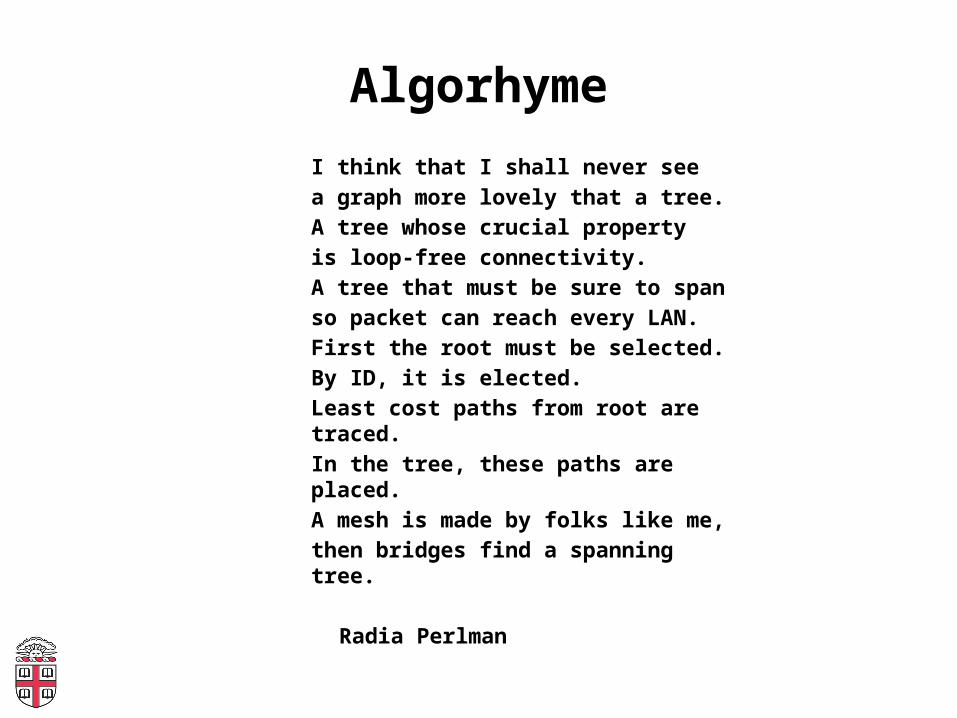
AlgorhymeI think that I shall never seea graph more lovely that a tree.A tree whose crucial propertyis loop-free connectivity.A tree that must be sure to spanso packet can reach every LAN.First the root must be selected.By ID, it is elected.Least cost paths from root are traced.In the tree, these paths are placed.A mesh is made by folks like me,then bridges find a spanning tree.
Radia Perlman

Limitations of Bridges
• Scaling– Spanning tree algorithm doesn’t scale– Broadcast does not scale– No way to route around congested links,
even if path exists
• May violate assumptions– Could confuse some applications that
assume single segment• Much more likely to drop packets• Makes latency between nodes non-uniform
– Beware of transparency

Multiple Paths
• L2: TRILL– L2 RBridges run link state protocol among
themselves– Add shim header, with destination RBridge,
hopcount
• L3: OSPF, IS-IS support multiple paths
• ECMP is possible in both

VLANs
• Company network, A and B departments– Broadcast traffic does not scale– May not want traffic between the two
departments– Topology has to mirror physical locations– What if employees move between offices?
b1
b2
a1
a2
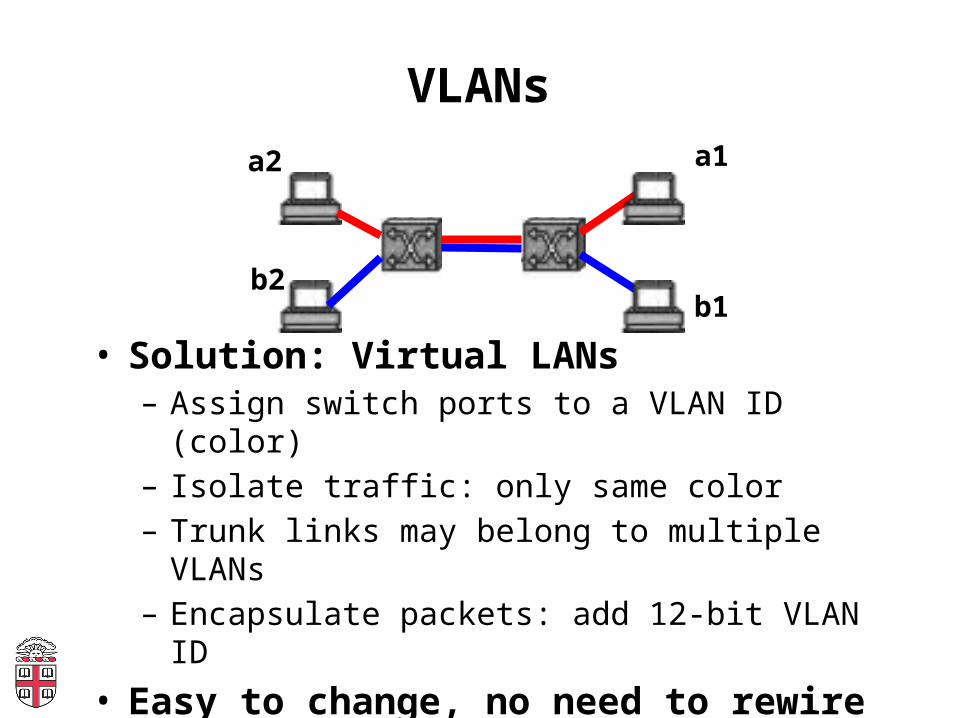
VLANs
• Solution: Virtual LANs– Assign switch ports to a VLAN ID (color)– Isolate traffic: only same color– Trunk links may belong to multiple VLANs– Encapsulate packets: add 12-bit VLAN ID
• Easy to change, no need to rewire
a2
b2
a1
b1

VLANs
• Limit the broadcast domain• Each VLAN becomes an IP subnet• Switches implement VLANs– First switch adds VLAN tag
• Port, MAC address, Protocol
– Last switch strips it off
• We will read a couple of interesting papers for next class on VLANs and campus networks

Switching
• Switches must be able to, given a packet, determine the outgoing port
• Some ways to do this:– Virtual Circuit Switching– Datagram Switching– Label switching– Source Routing

Virtual Circuit Switching
• Explicit set-up and tear down phases– Establishes Virtual Circuit Identifier on each link– Each switch stores VC table
• Subsequent packets follow same path– Switches map [in-port, in-VCI] : [out-port, out-
VCI]
• Also called connection-oriented model

Virtual Circuit Model• Requires one RTT before sending
first packet• Connection request contain full
destination address, subsequent packets only small VCI
• Setup phase allows reservation of resources, such as bandwidth or buffer-space– Any problems here?
• If a link or switch fails, must re-establish whole circuit
• Example: ATM

Datagram Switching
• Each packet carries destination address
• Switches maintain address-based tables– Maps [destination address]:[out-port]
• Also called connectionless model
Addr
Port
A 3
B 0
C 3
D 3
E 2
F 1
G 0
H 0
Switch 2
Datagram Switching
• No delay for connection setup• Source can’t know if network can
deliver a packet• Possible to route around failures• Higher overhead per-packet• Potentially larger tables at
switches

Source Routing
• Packets carry entire route: ports• Switches need no tables!– But end hosts must obtain the path
information
• Variable packet header
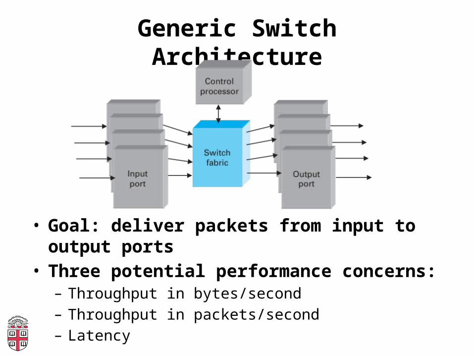
Generic Switch Architecture
• Goal: deliver packets from input to output ports
• Three potential performance concerns:– Throughput in bytes/second– Throughput in packets/second– Latency

Cut through vs. Store and Forward
• Two approaches to forwarding a packet– Receive a full packet, then send to output port– Start retransmitting as soon as you know output
port, before full packet
• Cut-through routing can greatly decrease latency
• Disadvantage– Can waste transmission (classic optimistic
approach)– CRC may be bad– If Ethernet collision, may have to send runt packet
on output link
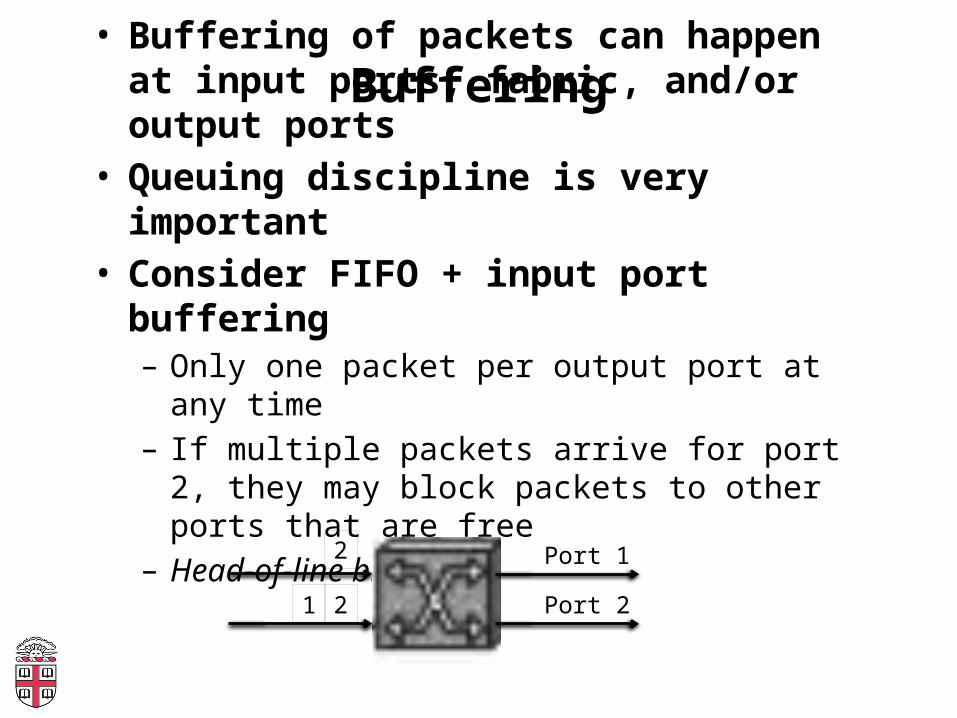
Buffering• Buffering of packets can happen at
input ports, fabric, and/or output ports
• Queuing discipline is very important
• Consider FIFO + input port buffering– Only one packet per output port at any
time– If multiple packets arrive for port 2, they
may block packets to other ports that are free
– Head-of-line blocking2
21
Port 1
Port 2

Shared Memory Switch
• 1st Generation – like a regular PC– NIC DMAs packet to memory over I/O bus– CPU examines header, sends to
destination NIC– I/O bus is serious bottleneck– For small packets, CPU may be limited too– Typically < 0.5 Gbps
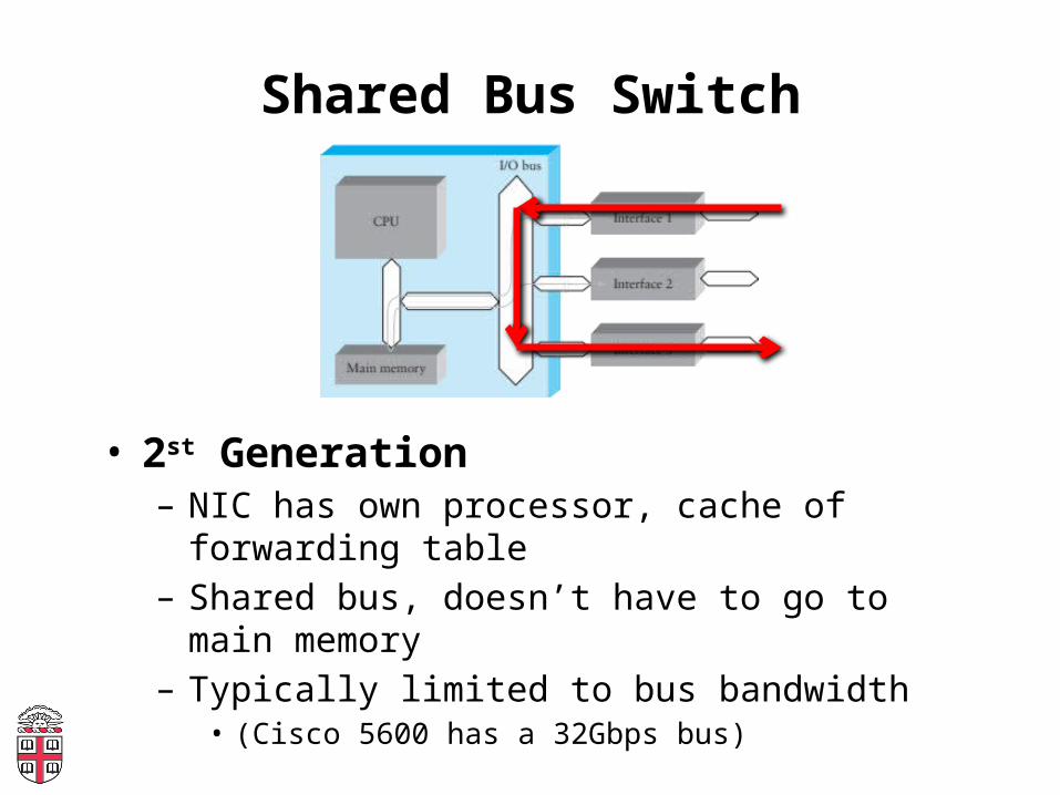
Shared Bus Switch
• 2st Generation– NIC has own processor, cache of
forwarding table– Shared bus, doesn’t have to go to main
memory– Typically limited to bus bandwidth
• (Cisco 5600 has a 32Gbps bus)

Point to Point Switch
• 3rd Generation: overcomes single-bus bottleneck
• Example: Cross-bar switch– Any input-output permutation– Multiple inputs to same output requires trickery– Cisco 12000 series: 60Gbps
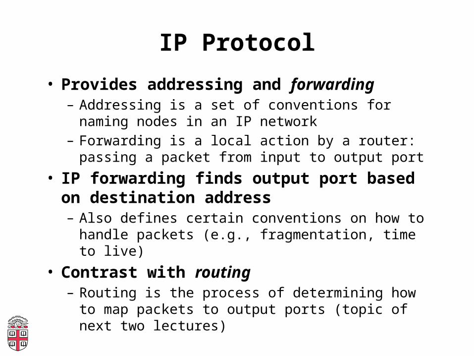
IP Protocol
• Provides addressing and forwarding– Addressing is a set of conventions for naming
nodes in an IP network– Forwarding is a local action by a router: passing
a packet from input to output port
• IP forwarding finds output port based on destination address– Also defines certain conventions on how to
handle packets (e.g., fragmentation, time to live)
• Contrast with routing– Routing is the process of determining how to
map packets to output ports (topic of next two lectures)

CIDR Forwarding Table
• Use longest prefix match• Default route: 0.0.0.0/0 (match any
address)• (also called Default Gateway)
Network Next Address18/8 212.31.32.5
128.148/16 212.31.32.4128.148.128/17 212.31.32.8
0/0 212.31.32.1
• Example Host: • address 212.31.32.15, net mask
212.31.32/24

Example
H1-> H2: H2.ip & H1.mask != H1.subnet => no direct path
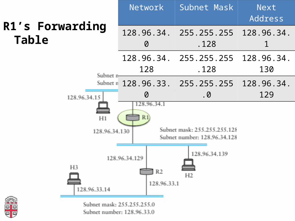
R1’s Forwarding Table
Network Subnet Mask Next Address
128.96.34.0 255.255.255.128 128.96.34.1
128.96.34.128 255.255.255.128 128.96.34.130
128.96.33.0 255.255.255.0 128.96.34.129

Translating IP to lower level addressesor… How to reach these local addresses?
• Map IP addresses into physical addresses– E.g., Ethernet address of destination host– or Ethernet address of next hop router
• Techniques– Encode physical address in host part of IP address
(IPv6)– Each network node maintains lookup table (IP-
>phys)

ARP – address resolution protocol• Dynamically builds table of IP to
physical address bindings for a local network
• Broadcast request if IP address not in table
• All learn IP address of requesting node (broadcast)
• Target machine responds with its physical address
• Table entries are discarded if not refreshed

ARP Ethernet frame format
• Why include source hardware address? Why not?
Obtaining Host IP Addresses - DHCP
• Networks are free to assign addresses within block to hosts
• Tedious and error-prone: e.g., laptop going from CIT to library to coffee shop
• Solution: Dynamic Host Configuration Protocol– Client: DHCP Discover to 255.255.255.255 (broadcast)– Server(s): DHCP Offer to 255.255.255.255 (why
broadcast?)– Client: choose offer, DHCP Request (broadcast, why?)– Server: DHCP ACK (again broadcast)
• Result: address, gateway, netmask, DNS server
Label Switching (MPLS)
• Packet carries a ‘label’: an identifier that the switch uses to select the outgoing port
• First switch decides on the label based on the packet
• The label switching table is set up in advance• Switch can also change the label before
forwarding– {in port, in label} -> {out port, out label}
• Makes for simpler switch design• Multiprotocol above and below
– Single forwarding algorithm