Download - CSNB234 ARTIFICIAL INTELLIGENCE
CSNB234CSNB234ARTIFICIAL INTELLIGENCEARTIFICIAL INTELLIGENCE
Chapter 5State Space Search
Chapter 5State Space Search
Instructor: Alicia Tang Y. C.

2
State Space Representation
A state space can be considered as consisting of a collection of points, each point corresponding to a state of a problem. So there will be as many number of points in the state space as the number of different possible states of the problem. Thus, a state space is the collection of all possible states, a problem can have. States can be represented as nodes of a tree. The searching of a goal node is by traversing the tree’s nodes using some well-established algorithms.

3
Defining A Search ProblemDefining A Search ProblemState Space
– is described by an initial state space a set of possible actions (operators) goal state
Path– is any sequence of actions that lead from a
state to another state and finally reached (hopefully) the goal node

4
Defining a Search ProblemDefining a Search Problem
Other considerations are:– Path cost: it is only relevant if there
exists more than one path leading to the goal state.
& certainly that we want the shortest path
– Goal test: it is applicable to single state problem, I.e. only one goal is found in the state space problem

5
Relationship between Initial states, actions and goal(s)
InitialStates
Actions Goal(s)
ControlStrategy
6
Why Why ‘‘SearchSearch’’??Search is an important (and
powerful ) aspect in AI problem solving
Search will– will help to explore alternatives in tree– will find sequence of steps in a
planning situation/caseAll goal-driven activities (such as
one used in B. C. reasoning) occur in a state space, and we call the problem a state space problem
7
Classical Search DomainsClassical Search Domains
8-PuzzleWater JugBlocks WorldTravelling SalesmanMazeChessTower of Hanoietc.

8
An Example of Search PreparationAn Example of Search Preparation
Initial State: The location of each of the 8-puzzle in one of the nine squares
Path cost: Each step costs 1 point, total path cost will be equal to the number of steps taken
Goal test: State matches the goal configuration (given board pattern)
Operators: blank moves [1] Left, [2] Right, [3] Up & [4] Down.
2
1
4
7
8
65
3
1
2
3
8 7
54
6InitialState
GoalState

9
SolutionTest Search ProcessSearch
Approaches
Blind
Heuristics
Optimisation
complete
partialCheck only
some alternatives
All possible solutions are
checked
Comparisonsstop
when all checked
Comparisons
optimal
Best among
alternatives
Onlypromisingsolutions
Stop whensolution is
goodenough
Goodenough
Generateimproved solutions
optimalStop when no improvement
is possible

10
Methods of Search (I)
Popular blind search methods are Depth-first Breadth-first Bi-directional Iterative deepening Depth-limited Uniform cost

11
Heuristic Search Hill-climbing Best-first Generate & test Induction Greedy search
Optimal Searching A* search
Methods of Search (II)

12
Depth-first– explores search tree branch by branch
Breadth-first– examines search tree row by row
Hill-climbing– it is depth first but most promising child node is
examined first Best-first
– expands the most promising partial path of all those so far discovered
A*– Best-first and Branch and bound algorithm
To becalculated
Decision required
Methods of search at the first glance
13
..…… Blind Blind……..
The entire search tree is examined in an orderly manner.
It can be classified as exhaustive or partial.
Two well-known partial methods are– breadth-first – depth-first

14
DEPTH-FIRST SEARCHDEPTH-FIRST SEARCH(DFS)(DFS)
A ~ begins at the root node and works downward to successively
deeper level.
This process continues until a solution is found or backtracking is forced by reaching a dead end.
Blind ....

15
DEPTH-FIRST SEARCHDEPTH-FIRST SEARCH
Delete FIRSTNODE from start of QUEUETake children of FIRSTNODEAdd to the front of QUEUEPut result in NEWQUEUE
Basic steps used
16
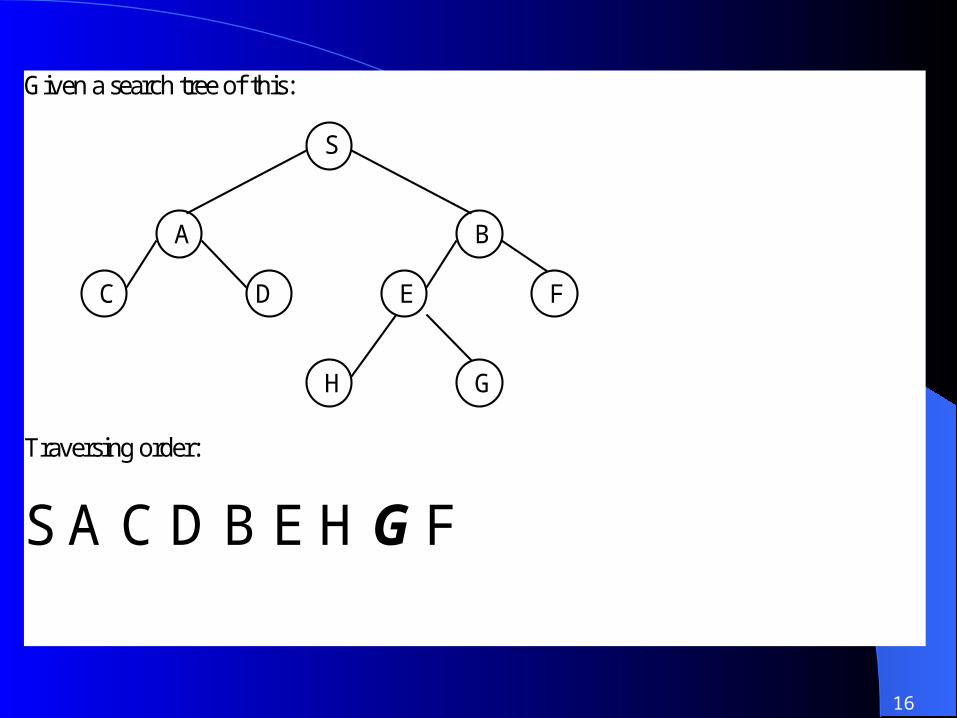
Given a search tree of this: S A B C D E F H G Traversing order:
S A C D B E H G F
17
BREADTH-FIRST SEARCH(BFS)
A ~ examines all the nodes in a search tree, beginning with the
root node.
The nodes in each level are examined completely before moving
to the next level.
18
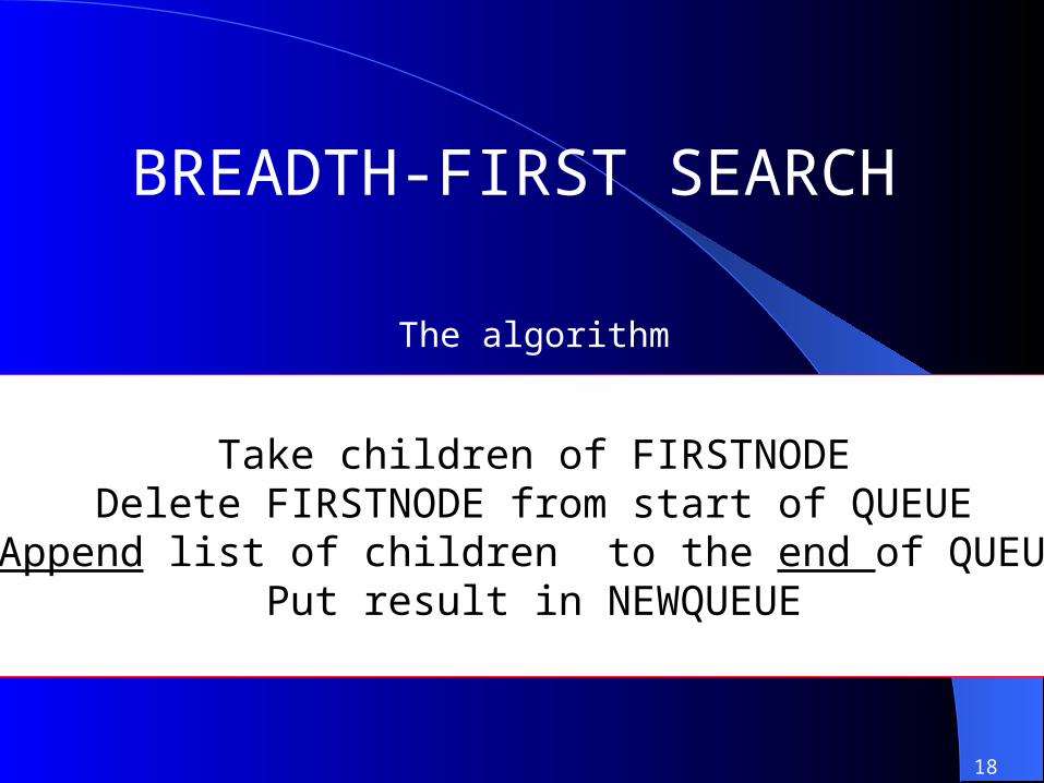
BREADTH-FIRST SEARCH
Take children of FIRSTNODEDelete FIRSTNODE from start of QUEUE
Append list of children to the end of QUEUEPut result in NEWQUEUE
The algorithm

19
Given a search tree of this: S A B C D E F H G Traversing order:
S A B C D E F H G

20
Heuristics Search Heuristics Search
Heuristics search is designed to reduce the amount of search for a solution.
It is based on rule-of-thumb principle.When a problem is presented, such as a
goal state is given, this approach tries to reduce the size of the search tree by pruning non promising or inferior nodes.
It can normally speed up the search process in obtaining a good enough solution.

21
Benefits of HeuristicsBenefits of Heuristics
It has inherent flexibilityIt is better when an optimal/best solution is
too costly to generate– even though it can only produce “good enough”
answerSimpler for decision maker to understand
(especially the managers)– because they think in the same way as
“heuristics” does
22
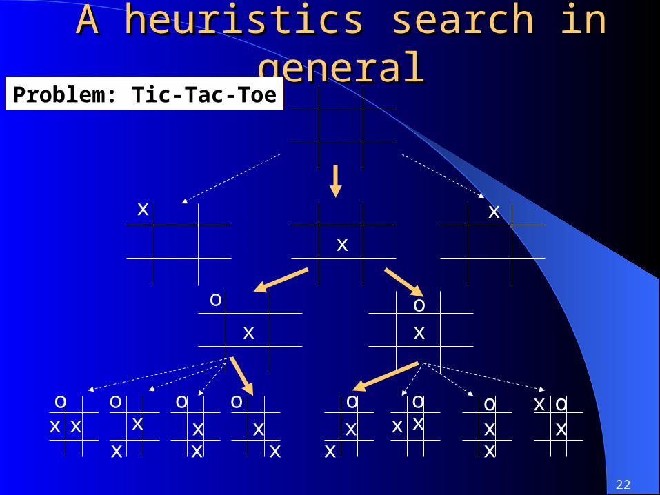
A heuristics search in generalA heuristics search in generalProblem: Tic-Tac-Toe
x
x
x
x x
ox x
ox
x
oxx
ox
x
ox
x
oxx
oxx
xxo
o o

23
Consider the Tic-Tac-Toe gameConsider the Tic-Tac-Toe game
Each nine first moves has eight possible responses, which in turn have seven continuing moves, and so on.
A simple analysis tells that the number of states to be considered in an exhaustive search is 9 * 8 * 7 *… or 9!
However, symmetry reduction in second level leads to only 12 * 7! (much smaller than above), further reduction in search
space will further reduce the number or search required
Blind search is surely not practical…

24
HILL-CLIMBING SEARCH
Delete FIRSTNODE from start of QUEUETake children of FIRSTNODE
Order children with most promising firstPlace them at the front of QUEUE
Put result in NEWQUEUE
Main steps used

25
HILL-CLIMBING SEARCH
Set Queue to be the List[StartNode]If Queue is non-empty, then:
Take the first element, FirstNode, in QueueIf FirstNode is a goal node, then:
Return FirstNodeOtherwise:
Delete FirstNode fro start of QueueTake children of FirstNodeOrder children with most promising firstPlace them at the front of QueuePut result in NewQueue
Otherwise: return failure(Recursive step) Repeat the procedure with NewQueue in place of Queue, let the result ofthis call be NodeReturn Node
A complete function:
26
Hill-ClimbingHill-Climbing
Hill-climbing combines depth-first search with a method for ordering the alternatives by measuring the probability of success at each decision point. In other word it tries to reach a goal by choosing those nodes which are predicted to be nearest to the goal. Quality measurements turn depth-first search into hill-climbing.
27
Earlier slide says that it is quite similar to depth-first blind search.
However, paths are not selected arbitrarily, but in relationship to their proximity to the desired goal (i.e. how close to it)
let’s take a look at this tree:– notice that there are numbers attached nodes
those are potential numbers of defects in a product
It is about fin ding the shortest h(n)
Hill-ClimbingHill-Climbing
28
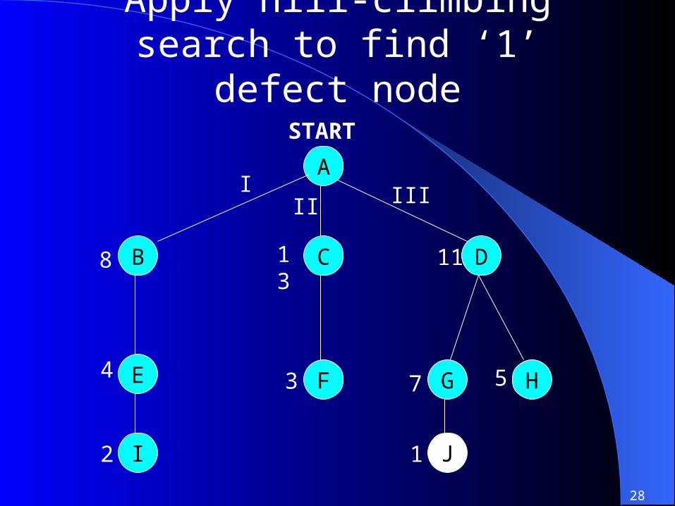
Apply hill-climbing search to find ‘1’ defect node
A
B C D
FE G H
I J
8
4
2
13
3
11
7 5
1
III III
START

29
Each production process I, II and III can continue for several stages.
If this is done by depth-first, it goes to I then to II and then to III .
In Hill-climbing method, nodes B, C and D are compared, and it starts in branch I (lowest, 8 here).
Since one defect was not found, backtracking is exercised to branch III. (branch III is done before II, why)?
The search goes to D and H; backtracking is then done and D, G, J path leads to the desired solution.
Path A--C--F was not visitedtherefore much time and cost are saved This is exactly the aims of ‘heuristics’!

30
Hill-climbingHill-climbing
Few more words on hill-climbing method: If we imagine the goal as the top of hill, h(n) as the difference in heights between n and the top, the hill-climbing procedure corresponds to climbing the hill by always going upwards.

31
Problems with hill-climbing:Problems with hill-climbing:
Foothill problem.– Go up to the top of a hill and not advancing
further. - misses the overall maximumPlateau problem.
– Problem with multidimensional problem space, i.e. no hill to climb (is flat). Gradient equals to zero. - not informative
Ridges.– Where there are steep slopes and the search
direction is not towards the way up (but side)
32
Some solutions to hill-Some solutions to hill-climbing problems are:climbing problems are:
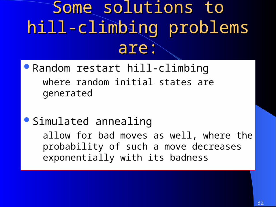
Random restart hill-climbing– where random initial states are generated
Simulated annealing– allow for bad moves as well, where the
probability of such a move decreases exponentially with its badness

33
BEST-FIRST SEARCHBased on some heuristics evaluation
function– More flexible than hill-climbing
An evaluation function is used to assign a score to each candidate node– Next move is made by selecting the best value
nodeIt expands the best partial path, for that It
could lead to “shortsighted” situation

34
BEST-FIRST SEARCHBest-first search has been used in such applications as
games and web crawlers In a web crawler, each web page is treated as a node,
and all the hyperlinks on the page are treated as unvisited successor nodes in the search space.
A crawler that uses best-first search generally uses an evaluation function that assigns priority to links based on how closely the contents of their parent page resemble the search query

35
BEST-FIRST SEARCH
Delete FIRSTNODE from start of QUEUETake children of FIRSTNODEAppend children to QUEUE
Order result with most promising firstPut ordered result in NEWQUEUE

36
Apply best-first search to find ‘3’ defect in a production
A
B C D
FE
G HI
J
8
14 16
13
23
11
7 5
3Traversing order (i.e. the search path) isA B D H G J
If hill climbing is used, the solution path will beA B E I D H G J (it is longer, less ‘intelligent’)
[A]
[B D C]
[D C E I]
[H G C E I]
[G C E I]
[J C E I]
[A]
[B D C]
[E I D C]
[I D C]
[D C]
[H G C]
[G C]
[J C]

37
Optimal SearchOptimal Search
Will produce optimal (best) answerBased on some optimisation functionMathematical functions are used
– for improvements – for “optimisation”

38
BRANCH AND BOUND ALGORITHM
One way to find optimal paths with less work is to use branch-and-bound.
It always keeps track of all partial paths contending for further consideration.
The shortest one is extended one level, creating as many new partial paths.
Next, these new paths are considered, along with the remaining old ones, again, the shortest is extended.
The process is repeated until the goal is reached along some path.

39
Branch-and-BoundBranch-and-BoundKeys to remember:
– To turn likely to certain, you have to extend all partial paths until they are as long or longer than the complete path. The reason is that the last step in reaching the goal may be long enough to make the supposed solution longer than one or more partial paths.
– It might be that only a tiny step would extend one of the partial paths to the solution node.
– To be sure that this is not so, instead of terminating when a path is found, you terminate when the shortest partial path is longer than the shortest complete path

40
An Example for B-N-BAn Example for B-N-B
S
D
A
B
E
F
G1515
The length of the completepath from S to G, S-D-E-F-G is 15.
Similarly, the length of the partial path S-D-A-B also 15and any additional movement along a branch will make it
longer than 15.Accordingly, there is no need to try S-D-A-B any further. Because it will be longerthan the complete path
already known.Only other paths emerging from S and from S-D-E have to be considered, as they may provide a shorter path.

41
To conduct a branch-and-bound search:
Form a one-element queue consisting of zero length path (only root node)– Until the first path in the queue terminated at
the goal node or the queue is empty,– remove the first path from the queue; create new paths by
extending the first path to all the neighbours of the terminal node
– reject all paths with loops– add the reaming new paths, if any, to the queue– sort the entire queue by path length with least-cost paths in
front
– If the goal is found, announce success; otherwise announce failure.
42
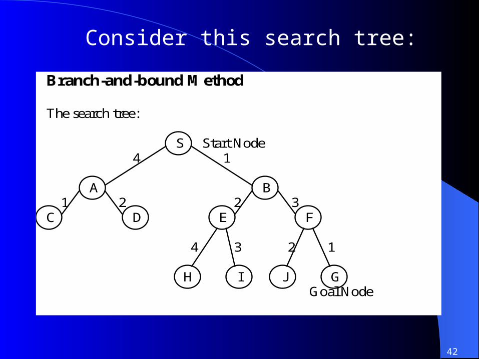
Branch-and-bound Method The search tree: S Start Node 4 1 A B 1 2 2 3 C D E F 4 3 2 1 H I J G Goal Node
Consider this search tree:

43
Search path to goal node:
[S(0)] [B(1) A(4)] [E(3) A(4) F(4)] [A(4) F(4) I(6) H(7)] [F(4) C(5) I(6) D(6) H(7)] [G(5) C(5) I(6) D(6) J(6) H(7)] Goal node reached and stopped.
Solution
Use your tie breaker solution
44
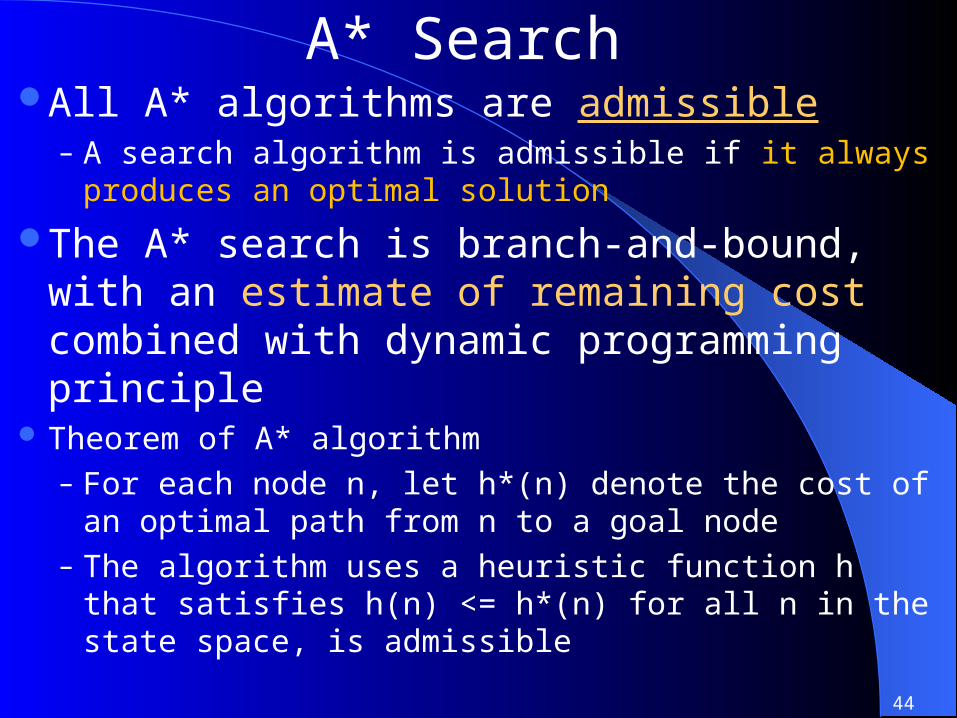
A* SearchAll A* algorithms are admissible
– A search algorithm is admissible if it always produces an optimal solution
The A* search is branch-and-bound, with an estimate of remaining cost combined with dynamic programming principle
Theorem of A* algorithm– For each node n, let h*(n) denote the cost of an
optimal path from n to a goal node– The algorithm uses a heuristic function h that
satisfies h(n) <= h*(n) for all n in the state space, is admissible
45
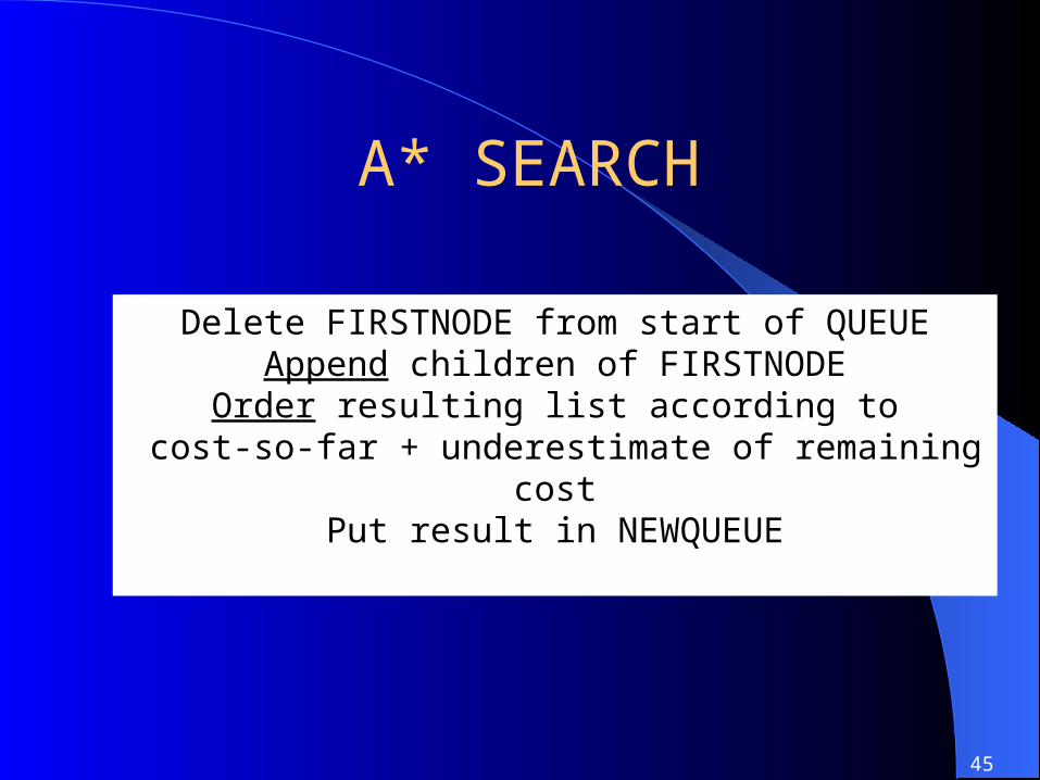
A* SEARCH
Delete FIRSTNODE from start of QUEUEAppend children of FIRSTNODEOrder resulting list according to
cost-so-far + underestimate of remaining costPut result in NEWQUEUE
46
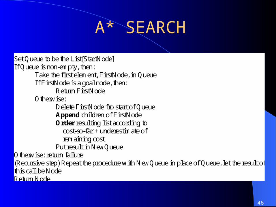
A* SEARCH
Set Queue to be the List[StartNode]If Queue is non-empty, then:
Take the first element, FirstNode, in QueueIf FirstNode is a goal node, then:
Return FirstNodeOtherwise:
Delete FirstNode fro start of QueueAppend children of FirstNodeOrder resulting list according to
cost-so-far + underestimate of remaining cost
Put result in NewQueueOtherwise: return failure(Recursive step) Repeat the procedure with NewQueue in place of Queue, let the result ofthis call be NodeReturn Node

47
To conduct a A* search: – Form a one-element queue consisting of zero length
path (only root node)– Until the first path in the queue terminated at the goal
node or the queue is empty,– remove the first path from the queue; create new paths by
extending the first path to all the neighbours of the terminal node
– reject all paths with loops– if two or more paths reach a common node, delete all
those paths except the one that reaches the common node with the minimum cost
– sort the entire queue by SUM of the path length and a lower-bound estimate of the cost remaining, with least-cost paths in front
– If the goal is found, announce success; otherwise announce failure.

48
Function definition in A*Function definition in A*
Consider the evaluation function f(n) = g(n) + h(n)
where n is any state in the search
g(n) is the cost from the start state
h(n) is the heuristic estimate of the cost
going from n state to goal node

49
Using Using A*A* in 8-puzzle problem in 8-puzzle problem
Figure 1 shows a start state and the first set of moves
2 8 3
1 6 47 5
2 8 3
1 6 47 5
2 8 3
16
47 5
2 8 3
1 6 47 5
START
First level ofThe tree search
Which one will the A* takes?& Why? On what basis it is chosen?
A1 A2 A3

50
1 2 3
8 47 5
To reach this GOAL state
6
Many levels of search and many solutions are possible to reach the goal state
What is the GOAL we wanted to achieve? i.e. what is the question?

51
Using Using A*A* in 8-puzzle problem in 8-puzzle problemFigure 2 : Three heuristics applied to states in the 8-puzzle
2 8 3
1 6 47 5
2 8 3
16
47 5
2 8 3
1 6 47 5
1 2 3
8 47 5
Recall the goal state5 6 0
3 4 0
5 6 0
Tiles out ofplace
Sum of distances out of place
6
2 * the no.of direct tilesreversals
These are potentialCriteria for the A* formula

52
Using Using A*A* in 8-puzzle problem in 8-puzzle problemFigure 3 : The heuristic f applied to states in the 8-puzzle
2 8 3
1 6 47 5
2 8 3
16
47 5
2 8 3
1 6 47 5
1 2 3
8 47 5
GOAL
2 8 3
1 6 47 5
g(n) = 0
g(n)=1
6 4 6f(n)f(n) = g(n) + h(n)where g(n) actual distance from n (cost from start state) h(n) the no. of tiles out of place
6

53
Exercise #1Exercise #1
List 4(four) criteria that are normally used to evaluate search
methods
Exercise #2Exercise #2
List 2(two) limitations of heuristics search methods

54
Answer to Exercise #1Answer to Exercise #1Completeness
– will the solution be eventually found? if there is one at all?
Space complexity– how much memory will it need or is necessary?
Time complexity– how long will it take to complete the search?
Optimality– will the search method find the highest quality of
solution path when there are several.

55
Supplementary SlidesSupplementary Slides

56
Properties of Search Algorithms
Breadth-first Depth-first A* Greedy
Complete Yes No Yes No Space Exponential Linear Exponential Linear
Time Exponential Exponential Exponential Exponential
Optimal Yes No Yes No

57
Bi-directional SearchBi-directional Search It searches both forward and backward in the
same state space (run simultaneously).It stops when the two moves meet in the
middle.
Start Goal
A schematic view of ~ that when a branch from the start node meets aBranch of the goal node, it stops
Blind Search..

58
Iterative Deepening (Korf 1987)
As depth-first search gets quickly into a deep level in the search space. Depth-first search can get lost deep in the search tree/graph. It may also stuck in infinite path that does not lead to a goal.
A compromise is to use a depth bound on depth-first :– the depth bound forces failure on a search
path once it gets below certain level
Blind Search..
59
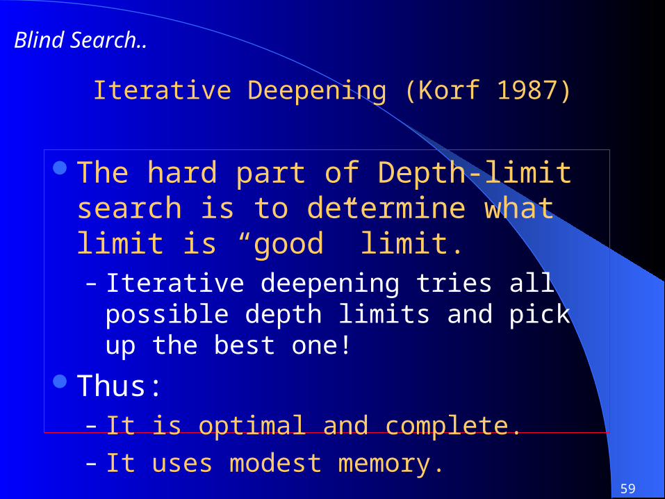
Iterative Deepening (Korf 1987)
The hard part of Depth-limit search is to determine what limit is “good” limit.– Iterative deepening tries all possible depth
limits and pick up the best one!Thus:
– It is optimal and complete.– It uses modest memory.
Blind Search..

60
Depth-Limited search
Similar to DFS, except that it avoids the pitfalls of DFS by imposing a cut off on the maximum depth of a given path
Drawback: if a chosen limit is too small, the scheme is not
“complete” optimality = no
Blind Search..

61
Uniform Cost SearchUniform Cost SearchWe learnt that BFS finds the
shallowest path leading to the goal state
uniform cost search modifies BFS by expanding only the lowest cost node (n)
the cost of a path should remain low but not decreasing hence the term “uniform”Note that if all step costs are equal, this is identical to BFS
Blind Search..
62
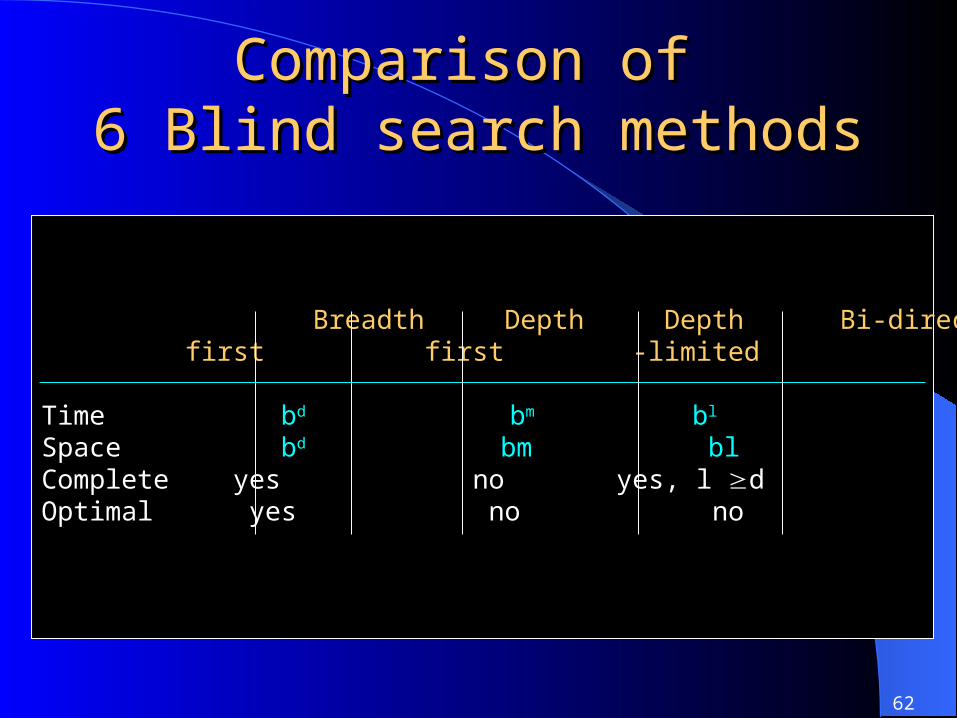
Comparison of Comparison of 6 Blind search methods6 Blind search methods
Breadth Depth Depth Bi-directional Iterative Uniform first first -limited cost
Time bd bm bl bd/2 bd bd
Space bd bm bl bd/2 bd bd
Complete yes no yes, l d yes yes yesOptimal yes no no yes yes yes
63
Induction
Induction means to generalise from a smaller version of the same problem
Two essential features– problem must be modelled in terms of the
associated data– induced result must be tested against real
examples
Heuristics …

64
Generate & Test The basic idea is to generate possible
solutions and devise a test to determine if the solutions are indeed good, i.e. acceptable.
Steps: add a specification criterion try to open a path that satisfies the specification determine whether the path is plausible, prune it
if it is not plausible move to the next path check whether all specifications have been
mentioned. If not, add the next specification and reiterate the steps by returning to first step
Heuristics …

65
Greedy SearchGreedy Search
There is a heuristic function, h(n), which serves to hold values of prediction of path-cost left to the goal
Greedy search is to minimise the estimated cost to reach the goal
Therefore, the node (state) closest to the goal will be expanded first
Heuristics …
66
Greedy SearchGreedy Search
It resembles DFS in the way that it follows a single path all the way to the goal, if there is no dead end
Thus, it is incomplete and not optimal
With good quality heuristic function, however, the space an time complexity can be reduced
Heuristics …


