
Data-Driven Processing In Sensor Networks
Jun YangDuke University
January 16, 2007

2
One possible type of sensor network
Small, untethered nodes with severe resource constraints– Sensors, e.g., light, moisture, …– Tiny CPU and memory– Battery power– Limited-range radio communication
• Usually dominates energy consumption
Nodes form a multi-hop network rooted at a base station– Base station has plentiful resources
and is typically tethered or at least solar-powered

3Duke Forest deployment
Use wireless sensor networks to study how environment affects tree growth in Duke forest– Collaboration with
Jim Clark (ecology) et al. since 2006

4Acknowledgement
Jim Clark, David Bell (ecology)
Alan Gelfand, Gavino Puggioni (statistics)
Adam Silberstein, Rebecca Braynard, Yi Zhang,Pankaj Agarwal, Carla Ellis, Kamesh Munagala (computer science)
Greg Filpus(undergrad)
National Science Foundation
Paul Flikkema (EE, NAU)

5
So, what do ecologists want?
Collect all data (to within some precision)– Probably the most boring database query
Fit stochastic models using data collected– Cannot be expressed as database queries
Very different from how I, a database researcher, would think about “querying data”– E.g., SQL, selection, join, aggregation…

6
Base station
Model-driven data collection: pull
Exploit correlation in sensor data– Representative: BBQ
[Deshpande et al., VLDB 2004]
Model p(X1, X2, …)
Sensor networkSensor network
x7 = ?
Additional observations: X9 = x9
Confidence interval not tight enough?
p(X7)
p(X7|X9 = x9)Confidence interval tightened
Answer correctness depends on model correctnessRisk missing the unexpected

7Data-driven philosophy
Models don’t substitute for actual readings– Particularly when we are still learning about
the physical process being monitored– Correctness of data collection should not
rely on correctness of modelsModels can still be used to optimize
collection

8Data-driven: push
Exploit correlation in data + put smarts in network– Representatives: Ken [Chu et al., ICDE 2006], Conch [Silberstein
et al., ICDE 2006, SIGMOD 2006]
Base station Model p(X(t)|o(t – 1), o(t –
2), …)
Sensor networkSensor networkCompare actual reading x(t) with model prediction E(X(t)| o(t – 1), o(t – 2), …)
Transmit o(t) such that kx(t) – E(X(t)|o(t), o(t – 1), …)k ·
Model p(X(t)|o(t – 1), o(t –
2), …)
Values transmitted at time t – 1
Differ by more than ?
Regardless of model quality, base station knows x(t) to within
Better model ) fewer transmissions

9
Temporal suppression example
Suppress transmission if |current reading – last transmitted reading|·– Model: X(t) = x(t – 1)
Effective when readings change slowly What about large-scale changes?
10
10
1010
10
10
10
10
10
10
10
10
10
Phenomenon is simple to describe, but all nodes transmit!
3030
30
30
30
30
2020
20
20
20
20
30 30
3030
30
30
30

10
Spatial suppression example
“Leader” nodes report for cluster Others suppress if
|my reading – leader’s reading|·– Model: Xme = xleader
Effective when nearby readings are similar
10
10
1010
10
10
10
10
10
10
10
10
10
leader
leader
leader
3030
30
30
30
30
2020
20
20
20
20
30 30
3030
30
30
30
Leaders always transmit!
Cluster 1
Cluster 2
Cluster 3

11
Combining spatial and temporal
Spatiotemporal suppression condition = ?Temporal AND spatial?
– I.e., suppress if both suppression conditions are met
– Results in less suppression than either!Temporal OR spatial?
– I.e., suppress if either suppression condition is met
– Base station cannot decide whether to set suppressed value to the previous value (temporal) or to the nearby value (spatial)!

12Outline
How to combine temporal and spatial suppressions effectively– Conch [Silberstein et al., SIGMOD 2006]
What to do about —the dirty little secret of suppression– BaySail [Silberstein et al., VLDB 2007]

13
Conch = constraint chaining
Temporally monitor spatial constraints (edges)
xi and xj change in similar ways ) temporally monitor edge difference (xi – xj)– “Difference” can be generalized
One node is reporter and the other updater– Reporter tracks (xi – xj) and
transmits it to base station if its value changes
– Updater transmits its value updates to reporter• I.e., temporally monitor remote input to the spatial
constraint
xj updatesupdater
(xi – xj) updates
reporteri
jConch edge

Recovering readings in Conch
Base station “chains” monitored edges to recover readings
Discretize values to avoid error stacking– [k, k+) ! k– Monitor discretized values exactly
• Discretization is the only source of error• No error introduced by suppression
14
x+1
x+1+2
x+1+2+3
x+1+2+3+4x
1 2
3
4
Chaining starting point; temporally monitored

15Conch example
10
10
1010
10
10
10
10
10
10
10
10
10
Temporally monitored start of chain
0
0
00
0 0 00
0
0
0
030
30
30
30
30
30–2010
2020
20
20
20
20
30 30
3030
30
30
30
Only “border” edges transmit to base stationCombines advantages of both temporal and spatial suppression

16Choosing what to monitor
A spanning forest is necessary and sufficient to recover all readings– Each edge is a temporally monitored spatial
constraint– Each tree root is temporally monitored
• Start of chain
(For better reliability, more edges can be monitored at extra cost)
Some intuition– Choose edges between correlated nodes– Do not connect erratic nodes
• Monitor them as singleton trees in the forest

17
Cost-based forest construction
Observe– In pilot phase, use any spanning forest to
collect data• Even a poor spanning forest correctly collects all
data
Optimize– Use collected data to assign monitoring costs
• # of rounds in which monitored value changes
– Build a min-cost spanning forest (e.g., Prim’s)Re-optimize as needed
– When actual costs differ significantly from those used by optimization

18Wavefront experiment
Simulate periodic vertical wavefronts moving across field, where sensors are randomly placed at grid points
Conch beats both pure temporal and pure spatial
Communication tree is a poor choice for monitoring;optimization makes a huge difference
Based on accounting of bytes sent/received on Mica2 nodes

19Conch discussion
Key ideas in Conch– Temporally monitor spatial constraints– Monitor locally—with cheap two-node spatial
models– Infer globally—through chaining– Push/suppress not only between nodes and
base station, but also among nodes themselves– Observe and optimize
Vision for ideal suppression– Number of reports / description complexity of
phenomenonWhat’s the catch?

20Outline
How to combine temporal and spatial suppressions effectively– Conch [Silberstein et al., SIGMOD 2006]
What to do about failures—the dirty little secret of suppression– BaySail [Silberstein et al., VLDB 2007]
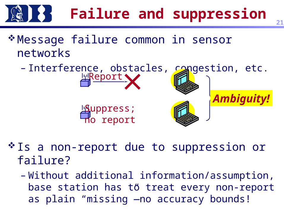
21Failure and suppression
Message failure common in sensor networks– Interference, obstacles, congestion, etc.
Is a non-report due to suppression or failure?– Without additional information/assumption,
base station has to treat every non-report as plain “missing”—no accuracy bounds!
Suppress; no report
Report
Ambiguity!

22A few previous approaches
Avoid missing data: ACK/Retransmit– Often supported by the communication layer– Still no guaranteed delivery ! does not help
with resolving ambiguityDeal with missing data
– Interpolation• Point estimates are often wrong or misleading• Uncertainty is lost—important in subsequent
analysis/action
– Use a model to predict missing data• Can provide distributions instead of point
estimates• But we have to trust the model!

23
BayBase: basic Bayesian approach
Model p(X|) with parameters – Do not assume is known– Any prior knowledge can be captured by p()
xobs: data received by base station Calculate posterior p(Xmis, |xobs)
– Joint distribution instead of point estimates– Quantifies uncertainty in model; model can be improved
( data-driven philosophy
Problem: non-reports are treated as generically missing– But most of them are “engineered”– Non-report no information!How do we incorporate knowledge of suppression scheme?

24BaySail
Bayesian Analysis of Suppression and Failure
Bayesian, data-drivenAdd back some redundancy Infer with redundancy and knowledge of
suppression scheme

25Redundancy strikes back
At app level, piggyback redundancy on each report
Counter: number of reports to base station thus far
Timestamps: last r timesteps when node reported
Timestamps+Direction Bits: in addition to the last r reporting timesteps, bits indicating whether each report is caused by (actual – predicted > or (predicted – actual >
A good CS trick!
Seems clumsy…
Why on earth?!

26
Suppression-aware inference
Redundancy + knowledge of suppression scheme ) hard constraints on Xmis
– Temporal suppression with = 0.3, prediction = last reported
– Actual: (x1, x2, x3, x4) = (2.5/sent, 3.5/sent, 3.7/suppressed, 2.7/sent)
– Base station receives: (2.5, nothing, nothing, 2.7)– With Timestamps (r=1)
• (2.5, failed, suppressed, 2.7)• |x2 – 2.5| > 0.3; |x3 – x2| · 0.3; |2.7 – x2| > 0.3
– With Timestamps+Direction Bits (r=1)• (2.5, failed & under-predicted, suppressed, 2.7 & over-
predicted)• x2 – 2.5 > 0.3; –0.3 · x3 – x2 · 0.3; x2 – 2.7 > 0.3
– With Counter• One suppression and one failure in x2 and x3; not sure
which• A very hairy constraint!
Posterior: p(Xmis, |xobs), with Xmis subject to constraints

27
Benefit of modeling/redundancy
x2
x3
???
x3
x2
x3
x2
x3
x2
Just data
No knowledge of suppression
Knowledge of suppression & Timestamps
Bayesian, model-basedAR(1) with uncertain parameter
x2
x2 2 [2.2, 3.0]
x 3 2 [x 2 – 0
.3, x 2 + 0.3]
Knowledge of suppression & Timestamps+Direction Bits
x3
x2
x2 > 3.0
x 3 2 [x 2 – 0
.3, x 2 + 0.3]x3
x2
BayBase
BaySail
BaySail

28
Redundancy design considerations
Benefit: how much uncertainty it helps to remove– Counter can cover long periods, but helps very little in
bounding particular values
Energy cost– Counter < Timestamps < Timestamps+Direction Bits
Complexity of in-network implementation– Coding app-level redundancy in TinyOS was much
easier than finding the right parameters to tune for ACK/Retransmit!
Cost of out-of-network inference– May be significant even with powerful base stations!

29Inference
Arbitrary distributions & constraints: difficult in general– Monte Carlo methods generally needed– Various optimizations apply under different conditions
A simplified soil moisture model: ys, t = ct+ ys, t –
1+es, t
– ct is a series of known precipitation amounts
– Cov(Ys, t , Ys’, t’) = 2 (|t – t’|/(1 – 2)) exp(– ks – s’k)
– 2 (0, 1) controls how fast moisture escapes soil– controls the strength of the spatial correlation over
distance
Given yobs, find p(Ymis, , 2, |yobs) subject to constraints
Gibbs sampling– Markovian ) okay to sample each cluster of missing
values in turn– Gaussian + linear constraints ) efficient sampling
methods

30Inference cost
>100£ speed-up!Major reason for adding the direction bits
translate to “|…| > ” constraints (disjunction); difficult to work with; naïve technique generates lots of rejected samples translate to a set of linear constraints; use [Rodriguez-Yam, Davis, Scharf 2004] and there are no rejections
Timestamps
Timestamps+Direction Bits

31
Energy cost vs. inference quality
ACK is not worth the trouble!
Sampling is okay in terms of cost, but has trouble with accuracy
Suppression-aware inference with app-level redundancy is our best hope to get higher accuracy
30% message failure rate
Roughly 60% suppression
Cost: bytes transmitted (including any message overhead)
Quality: size of 80% high-density region
32BaySail discussion
Suppression vs. redundancy– Goal of suppression was to remove redundancy– Now we are adding redundancy back—why?– Without suppression, we have to rely on naturally
occurring redundancy $ want to control where redundancy is needed, and how much
Many interesting future directions– Dynamic, local adjustments to and degree of
redundancy– In-network resolution of suppression/failure– Failure modeling– Provenance: is publishing received/interpolated
values enough?

33Concluding remarks
Data-driven approach– Use model to optimize, not to substitute for real data ! suppression– Quantify uncertainty in models; use data to learn/refine ! Bayesian
Conch: suppression by chaining simple spatiotemporal models
BaySail: suppression-aware inference with app-level redundancy to cope with failure (suppression’s dirty little secret)
This model-based stuff is not just for statisticians!– Cost-based optimization– Interplay between system design and statistical inference– Representing and querying data with uncertainty
All models are wrong, but some models are useful— George Box

34
Thanks!
Duke Database Research Grouphttp://www.cs.duke.edu/dbgroup/

35Related work
Sensor data acquisition/collection– BBQ [Deshpande et al. VLDB 2004], Snapshot [Kotidis ICDE
2005], Ken [Chu et al. ICDE 2006], PRESTO [Li et al. NSDI
2006], contour map [Xue et al. SIGMOD 2006] , …Sensor data cleaning
– ESP [Jeffery et al. Pervasive 2006], SMURF [Jeffery et al.
VLDB 2006], StreamClean [Khoussainova et al. MobiDE
2006], …Uncertainty in databases
– MYSTIQ [Dalvi & Suciu VLDB 2004], Trio/ULDB [Benjelloun
et al. VLDB 2006], MauveDB [Deshpande & Madden SIGMOD
2006], factors [Sen & Deshpande ICDE 2007], …

36Conch redundancy
Monitor more edges/nodes!
bc
d
a5
10
7
8
bc
d
a5
10
9
8
d = a + 5 + 10 andd = a + 9 + 8 cannot both be true!A failure occurred—but where?
Maximize:
Subject to:
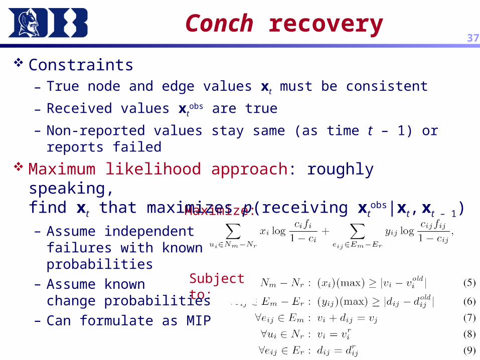
37Conch recovery
Constraints– True node and edge values xt must be consistent
– Received values xtobs are true
– Non-reported values stay same (as time t – 1) or reports failed
Maximum likelihood approach: roughly speaking,find xt that maximizes p(receiving xt
obs|xt, xt – 1) – Assume independent
failures with known probabilities
– Assume known change probabilities
– Can formulate as MIP

38
BaySail: infer with spatial correlation
Spatial correlation definitely helps!– Can you tell which nodes got less help?
1 2 3
4 5 6
7 8 9
3x3 Grid

Error stacking39
4.0
5.06.0
x+1
x+1+2
x+1+2+3
x
1 2
3
Chaining starting point; temporally monitored
3.0
4.0
5.06.0
1.0 1.0 1.0
3.0
4.9
6.88.7
1.9 1.9 1.9
3.01.0 1.0 1.0
4.0
5.06.0
3.01.0 1.0 1.0
Suppressed because |1.9 – 1.0| · = 1 Errors stack: 0.9+0.9+0.9 = 2.7!

Discretization40
4
56
x+1
x+1+2
x+1+2+3
x
1 2
3
Chaining starting point; temporally monitored
3.0
4.0
5.06.0
1 1 1
3.0
4.9!48.7!8
1 2 2
31 1 1
4
68
31 2 2
Transmitted
6.8!6

Gibbs sampling
Initialize (0), (0), (0) from prior; i à 1Loop:Draw ymis
(i) from p(Ymis|(i – 1), (i – 1), (i – 1), yobs)subject to constraints on
Ymis
Draw (i) from p(| ymis(i), (i – 1), (i – 1), yobs)
Draw (i) from p(| ymis(i), (i), (i – 1),
yobs)
Draw (i) from p(| ymis(i), (i), (i), yobs)
Record ymis(i), (i),(i),(i)
i à i + 1; repeat the loop
41


